Determination of the Joint Confidence Region of Optimal Operating Conditions in Robust Design by Bootstrap Technique

Abstract

Robust design has been widely recognized as a leading method in reducing variability and improving quality. Most of the engineering statistics literature mainly focuses on finding point estimates of the optimum operating conditions for robust design. Various procedures for calculating point estimates of the optimum operating conditions are considered. Although this point estimation procedure is important for continuous quality improvement, the immediate question is “how accurate are these optimum operating conditions?” The answer for this is to consider interval estimation for a single variable or joint confidence regions for multiple variables.

In this paper, with the help of the bootstrap technique, we develop procedures for obtaining joint confidence regions for the optimum operating conditions. Two different procedures using Bonferroni and multivariate normal approximation are introduced. The proposed methods are illustrated and substantiated using a numerical example.

Keyword: Bootstrap; quality improvement; robust design; optimization; response surface.

1 Introduction

Robust design has been widely recognized as a leading method in reducing variability in the quality characteristic and improving quality. It is also recognized that quality improvement activities are most efficient and cost-effective when implemented during the design stage. Because of their practicability, robust design techniques have found increased applications in many manufacturing industries. Many industries are of great interest in the potential for applying robust design principles and are seeking a role in the information revolution with robust design at its core.

The primary goal of robust design is to minimize variation in the quality characteristic of interest while keeping a process mean at the customer-identified target value. In order to achieve this goal, Taguchi (1986) introduced a systematic method for applying experimental design, which has become known as robust design. Even though the ad hoc robust design methods suggested by Taguchi remain controversial due to various mathematical imperfections, there is no serious disagreement among engineering researchers and practitioners about his basic philosophy. The controversy surrounding Taguchi’s assumptions, his experimental design, and his experimental analysis has been well addressed by Leon et al. (1987), Box (1988), Box et al. (1988), Nair (1992), and Tsui (1992). Consequently, researchers have closely examined alternatives using well-established statistical tools from traditional theories of experimental designs. In an early attempt of such research, Vining and Myers (1990) introduced the dual response approach based on a response surface methodology (RSM) as a superior alternative for modeling process relationships by separately estimating the response functions of the process mean and variance. The mean target value and variance of the target value are assumed to be polynomial functions of the various possible design points. Multiple experiments are conducted at the various design points in order to obtain estimates of the mean and variance of the target value at the various design points. Then, given these estimates, the coefficients for the response surface functions are estimated using standard regression techniques and the functions are assumed to hold continuously and therefore for points between the design points considered during the experiments. Vining and Myers (1990) then obtain the optimal design point (usually somewhere between those used during the experiment) by minimizing an objective function that penalizes mean bias and variance. Thus, it achieves the primary goal of robust design by minimizing the process variance while adjusting the process mean at the target.

However, Lin and Tu (1995) pointed out that the robust design solutions obtained from the dual response model may not necessarily be optimal since this model forces the process mean to be located at the target value and proposed the mean-squared-error model, relaxing the zero-bias assumption. While allowing some process bias, the resulting process variance is less than or at most equal to the variance obtained from the model proposed by Vining and Myers (1990); hence, the mean-squared-error model may provide better (or at least equal) robust design solutions if the zero-bias assumption is not required. The robust design approach to determining optimum values has been further studied by several researchers, including Borror and Montgomery (2000), Scibilia et al. (2003), Govindaluri et al. (2004), Lee et al. (2005), Kim et al. (2005), Lee and Park (2006), Lee et al. (2007a), and Lee et al. (2007b).

As afore-mentioned, the majority of the research on robust design modelling have focused on methodological development of models for optimizing operating conditions. Although this is critically important for continuous quality improvement, the immediate question is “how accurate are these optimum operating conditions?” To the best of our knowledge, the answer for this question has not been properly addressed in industrial applications of dual response surface methods. We can consider interval estimation for a single variable or joint confidence regions for multiple variables as an answer for this question.

With the help of the bootstrap technique, we develop procedures for obtaining joint confidence regions for the optimum operating conditions. The single response surface approach uses the method of least squares to obtain the adequate single response functions, while the squared-loss approach uses two surfaces for process mean and variance. For the single response surface approach, the variance-covariance matrix of the regression coefficients can be easily obtained, so the derivation of the joint confidence region for optimum conditions is straightforward. For more details, see Myers and Montgomery (2002). With two response functions, however, it is quite difficult to obtain the variance-covariance matrix of the regression coefficients for both the mean and variance responses, particularly when the sample size is not large. This difficulty can be overcome by using bootstrap techniques. In an era of powerful computers, computer-intensive methods such as the bootstrap technique promise to be one of the mainstays of applied response surface methodology and engineering statistics in the years ahead.

This paper is organized as follows. The basics of robust design are introduced in Section 2. The bootstrap approach to determining joint confidence region for the optimum conditions is described in Section 3, followed by a case study in Section 4 and the paper ends with concluding remarks in Section 5.

2 Robust design based on response surface

We consider a system with a response $Y$. This response depends on the levels of $k$ control factors $\mathbf{x}=(x_{1},x_{2},\ldots,x_{k})$. The following assumptions are generally made:

• The response $Y$ depends on $\mathbf{x}$. Thus, $Y$ can be viewed as a function of $\mathbf{x}$, that is, $Y=F(x_{1},x_{2},\ldots,x_{k})$. But, the functional structure $F(\cdot)$ is either unknown or very complicated.

• The levels of the control factor $x_{i}$ for $i=1,2,\ldots,k$ are continuously quantitative.

• The levels of the control factor $x_{i}$ for $i=1,2,\ldots,k$ can be controlled by the experimenter.

Following Vining and Myers (1990), the mean and variance response functions (surfaces) can be written as

$${M}(\mathbf{x}) ={\beta}_{0}+\sum_{i=1}^{k}{\beta}_{i}x_{i}+\sum_{i=1}^{k}{\beta}_{ii}x_{i}^{2}+\sum_{i<j}^{k}{\beta}_{ij}x_{i}x_{j}+\epsilon_{m}$$

and

$${V}(\mathbf{x}) ={\gamma}_{0}+\sum_{i=1}^{k}{\gamma}_{i}x_{i}+\sum_{i=1}^{k}{\gamma}_{ii}x_{i}^{2}+\sum_{i<j}^{k}{\gamma}_{ij}x_{i}x_{j}+\epsilon_{v},$$

respectively, where $\mathbf{x}=(x_{1},x_{2},\ldots,x_{k})$. To find the fitted response surfaces given above, we must regress the mean response ${M}(\mathbf{x})$ and the variance response ${V}(\mathbf{x})$ on the control factors, $x_{1},x_{2},\ldots,x_{k}$. Hence, we must estimate the mean and variance responses at each design point. The most popular estimation method is to find the maximum likelihood estimates, assuming that the error variables $\epsilon_{m}$ and $\epsilon_{v}$ are normally distributed. Suppose that $n$ replicates are taken at the $i$th design point. Let $Y_{ij}$ represent the $j$th response at the $i$th design point where $i=1,2,\ldots,k$ and $j=1,2,\ldots,n$. The most popular estimators of the location and scale parameters are mean and variance, respectively. The maximum likelihood estimates of the mean and variance at the $i$th design point are the sample mean and variance as shown below.

$$\overline{Y}_{i}=\frac{1}{n}\sum_{j=1}^{n}Y_{ij}\mathrm{~{}~{}and~{}~{}}S^{2}_{i}=\frac{1}{n-1}\sum_{j=1}^{n}(Y_{ij}-\overline{Y}_{i})^{2}.$$

Let $\hat{M}(\mathbf{x})$ and $\hat{V}(\mathbf{x})$ represent the fitted response functions for the mean and variance of the response $Y$, respectively. Assuming a second-order polynomial model for the response functions, we get

$$\hat{M}(\mathbf{x})=\hat{\beta}_{0}+\sum_{i=1}^{k}\hat{\beta}_{i}x_{i}+\sum_{i=1}^{k}\sum_{j=i}^{k}\hat{\beta}_{ij}x_{i}x_{j}$$ (1)

and

$$\hat{V}(\mathbf{x})=\hat{\gamma}_{0}+\sum_{i=1}^{k}\hat{\gamma}_{i}x_{i}+\sum_{i=1}^{k}\sum_{j=i}^{k}\hat{\gamma}_{ij}x_{i}x_{j}.$$ (2)

We use the sample mean and variance of $Y$ to estimate the process mean $\hat{M}(\mathbf{x})$ and variance $\hat{V}(\mathbf{x})$, respectively.

The main goal of robust design is to obtain the optimum operating conditions of control factors, $x_{1},x_{2},\ldots,x_{k}$, and this can be achieved by employing the following squared-loss optimization model:

$$\mathrm{minimize~{}}\big{\{}\hat{M}(\mathbf{x})-T_{0}\big{\}}^{2}+\hat{V}(\mathbf{x})$$

subject to

$$x_{j}\in[L_{j},U_{j}]\mathrm{~{}~{}for~{}}j=1,2,\ldots,k,$$

where $T_{0}$ is the customer-identified target value for the quality characteristic of interest, and the constraint specifies the feasible joint region of operating covariates given by $\mathbf{x}=(x_{1},x_{2},\ldots,x_{k})$. When factorial designs with $k$ levels are used, the constraint becomes $x_{j}\in[L_{j},U_{j}]\mathrm{~{}for~{}}j=1,2,\ldots,k$. The control factors ($x_{j}$) solving the optimization problem above are the optimal design point estimates.

When considering the process variance on the left hand side of the regression model in (2), one often uses the log-transformed values of the sample variances, i.e., $\log(S_{i}^{2})$, since a linear model for the variance process does not guarantee that the predicted values are always positive; see Myers and Montgomery (2002). Using the log-transform, we can avoid the problem of the negative estimates in the variance process. After estimating the logarithm of the process variance, ${V}_{\log}(\mathbf{x})$, we can obtain the optimal operating conditions by minimizing

$$\{\hat{M}(\mathbf{x})-T_{0}\}^{2}+\exp\big{(}\hat{V}_{\log}(\mathbf{x})\big{)}$$

subject to

$$x_{j}\in[L_{j},U_{j}]\textrm{~{}~{}for~{}~{}}j=1,2,\ldots,k.$$

It is noteworthy that the following dual-response optimization model proposed by Vining and Myers (1990) can also be used for optimization purposes:

$$\mathrm{minimize~{}}\hat{V}(\mathbf{x})$$

subject to

$$\hat{M}(\mathbf{x})=T_{0}\textrm{~{}~{}and~{}~{}}x_{j}\in[L_{j},U_{j}]\textrm{~{}~{}for~{}~{}}j=1,2,\ldots,k.$$

However, the dual-response model strictly imposes a zero-bias condition while the squared-loss model allows some bias (i.e., absolute value of the difference of $\hat{M}(x)$ and $T_{0}$). This squared-loss model often results in less variability, and will be the focus of this paper. For detailed information regarding the squared-loss model, readers may refer to Lin and Tu (1995).

3 Joint Confidence Region using Bootstrapped Samples

The bootstrap technique was first developed by Efron (1979) and this method has become one of the most popular computer-intensive statistical methods. The technique is simple yet powerful. The key idea is to retake samples from the original data in order to create re-sampled data sets from which the variability of the quantities of interest can be assessed without long and error-prone analytical calculations.

As afore-mentioned, unlike the single response surface method, it is quite difficult to obtain the theoretical variance-covariance matrix of the regression coefficients for both the mean and variance responses when two response functions are considered. The alternative is to calculate the statistic of interest from simulated data sets using the Bootstrap re-sampling technique. We denote such a simulated data set as $Y_{ij}^{*}$. It is standard to let the superscript notation (^∗) denote a bootstrapped or re-sampled value. The statistic of interest (optimum operating conditions) is calculated with a simulated data set. By simulating $B$ times, we obtain $B$ simulated optimum operating conditions. Using these conditions, we can obtain the joint confidence region of the optimum operating conditions of control factors. The bootstrap algorithm is as follows:

For $b=1,2,\ldots,B$:

1. Draw $Y_{i1}^{*},Y_{i2}^{*},\ldots,Y_{in}^{*}$ with replacement from $Y_{i1},Y_{i2},\ldots,Y_{in}$ for $i=1,2,\ldots,k$.

2. Find the optimum operating conditions using the above data set. We denote this as $(\hat{x}_{1,b}^{\mathrm{oc*}},\hat{x}_{2,b}^{\mathrm{oc*}})$.

3. Repeat the above two steps for $b=1,2,\ldots,B$.

Then we obtain $B$ simulated optimum operating conditions $(\hat{x}_{1,b}^{\mathrm{oc*}},\hat{x}_{2,b}^{\mathrm{oc*}})$ for $b=1,2,\ldots,B$. There are several ways of finding the joint confidence regions using bootstrapped samples. For more details, the reader is referred to Hall (1992) and Davison and Hinkley (1997). Here we briefly introduce two methods:

1. The construction of a rectangular region using a Bonferroni argument.

2. The construction of an elliptical contour based on an approximation to the multivariate normal distribution.

In the following section, we describe these two methods using a numerical example with multi-filament microfiber tows.

4 A Case Study

A company produces multi-filament microfiber tows. We conduct an experiment to determine the quality effect of control covariates. For such products, the key control factors are polymer temperature ($x_{1,i}$) and polymer feeding speed ($x_{2,i}$). The diameter ($Y$) of the microfiber is the most important quality issue and its nominal target value is $T_{0}=50$ microns. The $3\times 3$ factorial design taken at each design point for $i=1,2,\ldots,9$ and $j=1,2,\ldots,10$ is shown in Table 1. Here, the variables $x_{1,i}$ and $x_{2,i}$ are centered and re-scaled from the natural variables so that $x_{1,i}$ and $x_{2,i}$ are in $[-1,1]$. We then obtain the estimate of the mean response, $\hat{M}(\mathbf{x})$, and the estimate of the log-transformed variance response, $\hat{V}_{\log}(\mathbf{x})$, as follows.

$$\hat{M}(\mathbf{x}) =51.741+7.750x_{1}+8.053x_{2}+20.262x_{1}^{2}+19.939x_{2}^{2}-0.038x_{1}x_{2}.$$

$$\hat{V}_{\log}(\mathbf{x}) =0.841-0.015x_{1}-0.068x_{2}+0.620x_{1}^{2}+0.421x_{2}^{2}-0.339x_{1}x_{2}.$$

By minimizing

$$\{\hat{M}(\mathbf{x})-50\}^{2}+\exp\big{(}\hat{V}_{\log}(\mathbf{x})\big{)}$$

subject to

$$|x_{1}|\leq 1\textrm{~{}~{}and~{}~{}}|x_{2}|\leq 1,$$

the optimum operating conditions are obtained as

$$\hat{\mathbf{x}}^{\mathrm{oc}}=(\hat{x}_{1}^{\mathrm{oc}},\hat{x}_{2}^{\mathrm{oc}})=(-0.168,-0.179).$$

Table 1: Data for case study example.

$i$		$x_{1,i}$	$x_{2,i}$		$Y_{ij}$					$\overline{Y}_{i}$	$S^{2}_{i}$
1		$-1$	$-1$		73.94	76.09	73.39	79.82	76.47
					73.43	76.89	77.55	77.12	74.79	75.949	4.263
2		$0$	$-1$		67.30	64.55	62.08	58.18	66.36
					63.49	63.56	65.91	65.61	65.05	64.209	6.853
3		$1$	$-1$		94.03	93.67	91.80	86.34	93.24
					91.45	91.19	87.71	90.33	92.71	91.247	6.390
4		$-1$	$0$		66.93	63.35	64.55	63.47	60.23
					62.58	62.63	63.45	66.29	65.47	63.895	3.922
5		$0$	$0$		51.23	51.03	53.16	52.84	50.06
					50.02	52.42	53.32	51.35	53.57	51.900	1.775
6		$1$	$0$		80.58	78.10	80.44	76.83	83.11
					84.45	78.70	77.04	81.00	79.27	79.952	6.181
7		$-1$	$1$		97.95	91.50	93.42	91.67	89.63
					92.10	86.82	95.48	92.01	97.35	92.793	11.631
8		$0$	$1$		80.76	77.86	81.10	77.31	76.53
					80.31	78.51	79.60	79.78	78.16	78.992	2.377
9		$1$	$1$		106.10	107.24	110.72	103.57	109.17
					108.48	110.41	106.80	108.58	108.31	107.938	4.495

Two methods, the construction of a rectangular confidence region using a Bonferroni argument and the construction of an elliptical confidence region based on a multivariate normal distribution, are used to find the joint confidence region for the optimum operating conditions. For each bootstrap data set $Y^{*}_{ij}$ where $i=1,2,\ldots,9$ and $j=1,2,\ldots,10$, we obtain the following simulated estimates of the optimum conditions as shown in Table 2.

Table 2: Simulated estimates of the optimum conditions from bootstrap data sets.

$b$	1	2	3	4	5	6	$\cdots$	999
$\hat{x}^{\mathrm{oc}*}_{1,b}$	$-0.268$	$-0.254$	$-0.154$	$-0.079$	$-0.207$	$-0.202$	$\cdots$	$-0.169$
$\hat{x}^{\mathrm{oc}*}_{2,b}$	$-0.141$	$-0.089$	$-0.207$	$-0.146$	$-0.207$	$-0.197$	$\cdots$	$-0.196$
$\hat{M}(\hat{\mathbf{x}}^{\mathrm{oc}*}_{b})$	$50.024$	$50.060$	$50.255$	$50.036$	$50.692$	$50.399$	$\cdots$	$50.503$

A Bonferroni argument can be used to find the rectangular confidence region. Suppose that $\theta$ is $d$-dimensional and the joint confidence region $C^{\alpha}=(C^{\alpha_{1}}_{1},C^{\alpha_{2}}_{2},\ldots,C^{\alpha_{d}}_{d})$ is rectangular, with the interval $C^{\alpha_{i}}_{i}=(\theta^{L}_{i},\theta^{U}_{i})$ for the $i$th component, where $i=1,2,\ldots,d$. Then we have

$$P(\theta\not\in C^{\alpha})=P\big{(}{\bigcup_{i=1}^{d}}\{\theta_{i}\not\in C^{\alpha_{i}}_{i}\}\big{)}\leq\sum_{i=1}^{d}P(\theta_{i}\not\in C^{\alpha_{i}}_{i})=\sum_{i=1}^{d}\alpha_{i}.$$

If we take $\alpha_{i}=\alpha/d$, then the region $C^{\alpha}$ covers at least $100(1-\alpha)$%. In our particular example, the region is two-dimensional, so we have $d=2$. If we want to find the 90% joint confidence region, we can use $\alpha_{1}=0.05$ and $\alpha_{2}=0.05$. To obtain the joint confidence, we need to find the confidence interval $C^{\alpha_{i}}_{i}$ for $i=1,2$. That is, we find the 95% confidence intervals of ${x}^{\mathrm{oc}}_{1,b}$ and ${x}^{\mathrm{oc}}_{2,b}$, separately. First, we will find the interval of ${x}^{\mathrm{oc}}_{1,b}$. For convenience, we denote ${x}^{\mathrm{oc}}_{1,b}$ as $\theta$ and the estimator of $\hat{x}^{\mathrm{oc}}_{1,b}$ as $T$. The realization of the estimator $T$ is denoted by $t$, and its bootstrap simulated values are denoted by $t^{*}$. To find the confidence interval, we need to estimate quantiles for $T-\theta$ and these are approximated using the bootstrap quantile of $t^{*}-t$. The $p$th quantile of $T-\theta$ is estimated by the $(B+1)p$th ordered value of $t^{*}-t$, that is $t^{*}_{[(B+1)p]}-t$. Then, as described in Davison and Hinkley (1997), an equi-tailed $100(1-\alpha_{1})$% confidence interval will have the following endpoints:

$$t-(t^{*}_{[(B+1)(1-\alpha_{1}/2)]}-t)\mathrm{~{}~{}and~{}~{}}t-(t^{*}_{[(B+1)\alpha_{1}/2]}-t).$$

In this particular bootstrap simulation, we used $B=999$. Thus, we have

$$t^{*}_{[(B+1)(1-\alpha_{1}/2)]}=t^{*}_{[975]}\mathrm{~{}~{}and~{}~{}}t^{*}_{[(B+1)(\alpha_{1}/2)]}=t^{*}_{[25]}.$$

Figure 1: Scatter plot of bootstrap results of the optimum operation conditions.

Similarly, we can find the confidence interval for ${x}^{\mathrm{oc}}_{2,b}$. Although the Bonferroni argument has a long history in statistics, it is well known that the Bonferroni joint confidence region is wider than what they should be at a given confidence level and it is therefore conservative. Also, with plausible likelihood function contours, a circular or elliptic shape could be more appropriate than a rectangular shape. One possible simple remedy for these deficiencies of the Bonferroni method is to use the classical normal-distribution approximation method. In our example, the region is two-dimensional, so a joint confidence region is an ellipse. If the $d$-dimensional estimator $\mathbf{T}$ of $\boldsymbol{\theta}$ is approximately multivariate normal, then it is well known that the quadratic quantity $Q$ shown below has an approximate $\chi^{2}_{d}$ distribution

$$Q(\boldsymbol{\theta})=(\mathbf{T}-\boldsymbol{\theta})^{\prime}\hat{\boldsymbol{\Sigma}}^{-1}(\mathbf{T}-\boldsymbol{\theta}),$$

where $\boldsymbol{\Sigma}$ is the estimated variance-covariance matrix of $\mathbf{T}$.

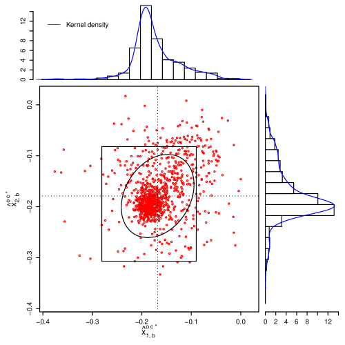
Figure 2: Blowup plot of Figure 1 with marginal histograms and kernel densities.

If $Q$ has exact chi-square quantiles $\chi_{d}^{2}(p)$, then a $100(1-\alpha)$% joint confidence region for $\boldsymbol{\theta}$ is

$$\{\boldsymbol{\theta}:Q(\boldsymbol{\theta})<\chi^{2}_{d}(1-\alpha)\}.$$

However, such chi-square quantiles are often unreliable, so it makes sense to use the bootstrap approximation of the distribution of $Q$ to find quantiles of $Q$. The bootstrap analogue of $Q$ is

$$Q^{*}(\mathbf{t})=(\mathbf{T}^{*}-\mathbf{t})^{\prime}{\boldsymbol{\hat{\Sigma}}^{*}}^{-1}(\mathbf{T}^{*}-\mathbf{t}),$$

which is calculated for each of the $B$ bootstrap samples and its calculation is denoted by $q^{*}$. If we denote the ordered bootstrap values by $q^{*}_{[1]},q^{*}_{[2]},\ldots,q^{*}_{[B]}$, then $100(1-\alpha)$% bootstrap joint confidence region is given by

$$\{\boldsymbol{\theta}:(\mathbf{t}-\boldsymbol{\theta})^{\prime}{\boldsymbol{\hat{\Sigma}}}^{-1}(\mathbf{t}-\boldsymbol{\theta})<q^{*}_{[(B+1)(1-\alpha)]}\}.$$

In the calculation of $Q^{*}$, we need to find the variance estimator ${\boldsymbol{\hat{\Sigma}}^{*}}$. One general way to obtain the value for ${\boldsymbol{\hat{\Sigma}}^{*}}$ is to calculate

$${\boldsymbol{\hat{\Sigma}}^{*}}=\frac{1}{I-1}\sum_{i=1}^{I}(\mathbf{t}_{i}^{**}-\mathbf{\bar{t}}^{**})(\mathbf{t}_{i}^{**}-\mathbf{\bar{t}}^{**})^{\prime},$$

where $\mathbf{\bar{t}}^{**}=(1/I)\sum_{k=1}^{I}\mathbf{t}_{k}^{**}$ and $\mathbf{t}_{1}^{**},\mathbf{t}_{2}^{**},\ldots,\mathbf{t}_{I}^{**}$ are calculated by bootstrap re-sampling from the bootstrap sample for each of the $B$ simulated samples. Since $\mathbf{t}_{i}^{**}$ are obtained by using bootstrap re-sampling of the bootstrapped sample, the double superscript notation (^∗∗) is used. Typically, $I$ is in the range between $50$ and $200$. In this example, we set $I=100$. For convenience, we denote

$$\boldsymbol{\theta}=({x}^{\mathrm{oc}}_{1},{x}^{\mathrm{oc}}_{2})^{\prime}\textrm{~{}and~{}}\mathbf{T}=(\hat{x}^{\mathrm{oc}}_{1},\hat{x}^{\mathrm{oc}}_{2})^{\prime}.$$

Figures 1 and 2 show the scatter plots of $B=999$ pairs of the optimum conditions based on the bootstrap samples. Figure 2 is the blowup plot of Figure 1 with the marginal histograms and kernel density estimates of $\hat{x}^{\mathrm{oc*}}_{1,b}$ and $\hat{x}^{\mathrm{oc*}}_{2,b}$. The values of the optimum conditions from the original sample is superimposed on the plot. The vertical dotted line is $\hat{x}^{\mathrm{oc}}_{1}=-0.168$ and the horizontal dotted line is $\hat{x}^{\mathrm{oc}}_{2}=-0.179$.

The rectangular region is the 90% joint confidence region based on Bonferroni simultaneous confidence intervals, while the 90% confidence elliptic region is based on the multivariate normal approximation. The bootstrap biases defined as

$$\frac{1}{B}\sum_{b=1}^{B}\hat{x}^{\mathrm{oc*}}_{i,b}-\hat{x}^{\mathrm{oc}}_{i}$$

for $i=1,2$ are $0.00208$ and $0.00411$, respectively. It is noteworthy that the rectangular confidence region deviates somewhat from the main body of the scatter plot downward and toward the left. This deviation comes from the bootstrap bias and skewness of the first and second components of the optimum operating conditions.

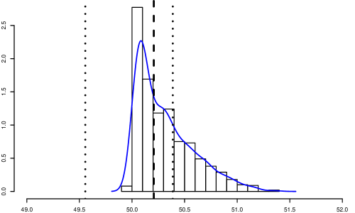
Figure 3: Histogram of the bootstrap mean response values.

We can also find the confidence interval of the mean response at the optimum conditions. Using this bootstrap technique, we can find the bootstrap estimates of the mean response at the optimum, that is, $\hat{M}(\hat{\mathbf{x}}^{\mathrm{oc}*}_{b})$. The mean response estimate at the optimum from the original sample is $50.30$. Using the simulated bootstrap samples, we can find the 90% bootstrap confidence interval, $(49.36,50.59)$. Figure 3 also shows the histogram of bootstrap mean response values, where the dotted vertical lines are the end points of the confidence interval and the vertical dashed line is the mean response estimate at the optimum from the original sample. The bias of the bootstrap estimate is 0.17. Because of this bias, we observe that the confidence interval moves toward the left.

5 Concluding remarks

In this paper, we developed methods of constructing joint confidence regions for optimum operating conditions using the bootstrap technique. Two different procedures were developed: A Bonferroni type procedure that constructed a rectangular region and multivariate normal approximation procedure that constructed an elliptical region. The proposed methods were illustrated and substantiated using a numerical example involving multi-filament microfiber tows.

References

- Borror and Montgomery (2000) Borror, C. M. and Montgomery, D. C. (2000). Mixed resolution designs as alternative to Taguchi inner/outer array designs for robust design problems. Quality and Reliability Engineering Inetrnational, 16, 1–11.
- Box (1988) Box, G. E. P. (1988). Signal-to-noise ratios, performance criteria, and transformations. Technometrics, 30, 1–17.
- Box et al. (1988) Box, G. E. P., Bisgaard, S., and Fung, C. (1988). An explanation and critique of Taguchi’s contributions to quality engineering. International Journal of Reliability Management, 4, 123–131.
- Davison and Hinkley (1997) Davison, A. C. and Hinkley, D. V. (1997). Bootstrap Methods and Their Application. Cambridge University Press.
- Efron (1979) Efron, B. (1979). Bootstrap methods: another look at the jackknife. Annals of Statistics, 7, 1–26.
- Govindaluri et al. (2004) Govindaluri, M. S., Shin, S., and Cho, B.-R. (2004). Tolerance optimization using the Lambert W function: an empirical approach. International Journal of Production Research, 42(16), 3235––3251.
- Hall (1992) Hall, P. (1992). The Bootstrap and Edgeworth Expansion. Springer-Verlag, New York.
- Kim et al. (2005) Kim, Y., Cho, B., Lee, M., and Kwon, H. (2005). Design optimization modeling for customer-driven concurrent tolerance allocation. In O. Gervasi, M. Gavrilova, V. Kumar, A. Laganá, H. Lee, Y. Mun, D. Taniar, and C. Tan, editors, Computational Science and Its Applications – ICCSA 2005, volume 3483 of Lecture Notes in Computer Science, pages 833–833. Springer Berlin / Heidelberg.
- Lee et al. (2005) Lee, M., Kwon, H., Kim, Y., and Bae, J. (2005). Determination of optimum target values for a production process based on two surrogate variables. In Computational Science and Its Applications–ICCSA 2005, volume 3483 of Lecture Notes in Computer Science, pages 833–833. Springer Berlin / Heidelberg.
- Lee et al. (2007a) Lee, M. K., Kwon, H. M., Hong, S. H., and Kim, Y. J. (2007a). Determination of the optimum target value for a production process with multiple products. International Journal of Production Economics, 107(1), 173 – 178. Special Section on Building Core-Competence through Operational Excellence.
- Lee and Park (2006) Lee, S. B. and Park, C. (2006). Development of robust design optimization using incomplete data. Computers & Industrial Engineering, 50, 345–356.
- Lee et al. (2007b) Lee, S. B., Park, C., and Cho, B.-R. (2007b). Development of a highly efficient and resistant robust design. International Journal of Production Research, 45, 157–167.
- Leon et al. (1987) Leon, R. V., Shoemaker, A. C., and Kackar, R. N. (1987). Performance measures independent of adjustment: An explanation and extension of Taguchi signal-to-noise ratio. Technometrics, 29, 253–285.
- Lin and Tu (1995) Lin, D. K. J. and Tu, W. (1995). Dual response surface optimization. Journal of Quality Technology, 27, 34–39.
- Myers and Montgomery (2002) Myers, R. H. and Montgomery, D. C. (2002). Response Surface Methodology. John Wiley & Sons, New York, 2nd edition.
- Nair (1992) Nair, V. N. (1992). Taguchi’s parameter design: A panel discussion. Technometrics, 34, 127–161.
- Scibilia et al. (2003) Scibilia, B., Kobi, A., Barreau, A., and Chassagnon, R. (2003). Robust designs for quality improvement. IIE Transactions, 35, 487–492.
- Taguchi (1986) Taguchi, G. (1986). Introduction to Quality Engineering. Asian Productivity Organization, White Plains, NY.
- Tsui (1992) Tsui, K. L. (1992). An overview of Taguchi method and newly developed statistical methods for robust design. IIE Transactions, 24, 44–57.
- Vining and Myers (1990) Vining, G. G. and Myers, R. H. (1990). Combining Taguchi and response surface philosophies: a dual response approach. Journal of Quality Technology, 22, 38–45.