Occupation numbers of the harmonically trapped few-boson system

Abstract

We consider a harmonically trapped dilute $N$-boson system described by a low-energy Hamiltonian with pairwise interactions. We determine the condensate fraction, defined in terms of the largest occupation number, of the weakly-interacting $N$-boson system ($N\geq 2$) by employing a perturbative treatment within the framework of second quantization. The one-body density matrix and the corresponding occupation numbers are compared with those obtained by solving the two-body problem with zero-range interactions exactly. Our expressions are also compared with high precision ab initio calculations for Bose gases with $N=2-4$ that interact through finite-range two-body model potentials. Non-universal corrections are identified to enter at subleading order, confirming that different low-energy Hamiltonians, constructed to yield the same energy, may yield different occupation numbers. Lastly, we consider the strongly-interacting three-boson system under spherically symmetric harmonic confinement and determine its occupation numbers as a function of the three-body “Efimov parameter”.

I Introduction

The weakly-interacting homogeneous Bose gas has been studied extensively in the literature bogo47 ; lee57 ; lee57a ; huan57 ; wu59 ; huge57 . Most commonly, the equation of state of the homogeneous Bose gas is expressed in terms of the square root of the dimensionless gas parameter $\rho[a_{s}(0)]^{3}$, where $\rho$ denotes the density and $a_{s}(0)$ the zero-energy $s$-wave scattering length. The leading order term is the mean-field energy and the lowest order correction accounts for quantum fluctuations. In an alternative approach huan57 ; bean07 ; detm08 ; tan08 , the ground state energy of $N$ bosons in a cubic box with periodic boundary conditions has been obtained by applying perturbation theory or the techniques of effective field theory to the weakly-interacting regime. As outlined by Lee, Huang and Yang lee57a , the latter approach must reproduce the equation of state of the weakly-interacting homogeneous Bose gas if the energies of the “subclusters” are summed up carefully.

In addition to the energy, other observables of the homogeneous weakly-interacting Bose gas have been considered. The condensate fraction $N_{0}/N$, i.e., the fraction of particles in the macroscopically occupied lowest momentum state, is a particularly interesting quantity since it can be measured experimentally. Furthermore, the connection between the condensate fraction and the superfluid fraction has been investigated in the literature, starting with the seminal works of London, Penrose and Onsager, and others lond38 ; penr56 ; atkins ; tilley . The condensate fraction has, as the energy per particle, been expanded in terms of the gas parameter $\rho[a_{s}(0)]^{3}$, $N_{0}/N=1-8/(3\sqrt{\pi})\sqrt{\rho[a_{s}(0)]^{3}}+\cdots$. Application of the local density approximation shows that the condensate fraction of the weakly-interacting Bose gas under spherically symmetric harmonic confinement scales as $N/N_{0}=1-5\sqrt{\pi}/8\sqrt{\rho(0)[a_{s}(0)]^{3}}+\cdots$, where $\rho(0)$ denotes the peak density dalf98 .

This work considers $N$ identical mass $m_{a}$ bosons under spherically symmetric harmonic confinement with angular trapping frequency $\omega$. For a review article of trapped gases, the reader is referred to Ref. blumereview . In the weakly-interacting regime, i.e., in the regime where the two-body $s$-wave scattering length $a_{s}(0)$ (expressed in units of $a_{\rm{ho}}$) and the product of the two-body effective range $r_{e}$ and $[a_{s}(0)]^{2}$ (expressed in units of $a_{\rm{ho}}^{3}$) are small, we determine expressions for the condensate fraction $N_{0}/N$; here, $a_{\rm{ho}}$ denotes the harmonic oscillator length, $a_{\rm{ho}}=\sqrt{\hbar/(m_{a}\omega)}$. For trapped systems, the condensate fraction is related to the largest eigen value of the one-body density matrix. In particular, the largest eigen value or occupation number of the one-body density matrix defines the condensate fraction. Our results are obtained by applying time-independent perturbation theory to the $N$-boson Hamiltonian with pairwise zero-range interactions characterized by $a_{s}(0)$ and $r_{e}[a_{s}(0)]^{2}$. The perturbative expressions are compared with highly accurate numerical results for Bose gases with $N=2-4$ that interact through a sum of short-range two-body model potentials. This comparison confirms that the leading-order term of the condensate depletion scales as $(N-1)[a_{s}(0)]^{2}$. At sub-leading order, a non-universal correction appears, i.e., a correction which is independent of $a_{s}(0)$ and $r_{e}$ and which is not needed to reproduce the energy of the finite-range system within an effective field theory approach john09 ; john12 .

For the two- and three-boson systems, we go beyond the weakly-interacting regime. For two harmonically trapped bosons that interact through a regularized zero-range interaction potential, we determine the occupation numbers as a function of the scattering length. For the three-boson system, we consider the unitary regime [$1/a_{s}(0)=r_{e}=0$] and determine the occupation numbers as a function of the three-body phase or Efimov parameter. The occupation numbers for the two- and three-body systems show “oscillatory behavior” in the positive energy regime if plotted as a function of the relative two-body energy and relative three-body energy, respectively. In the two-particle case, the oscillations are associated with the fact that the two-body $s$-wave phase shift changes by $2\pi$ as the two-body energy changes by about $2\hbar\omega$. In the three-particle case, in contrast, the oscillations are associated with the fact that the three-body Efimov phase goes through cycles of $2\pi$ as the three-body energy changes.

The remainder of this paper is organized as follows. Section II introduces the system Hamiltonian and defines the one-body density matrix and the occupation numbers. Section III discusses the occupation numbers of the trapped two-boson system. Section IV considers the weakly-interacting regime of the $N$-boson system. Section V considers the strongly-interacting three-boson system. Lastly, Sec. VI concludes. Mathematical details are relegated to Appendix A and Appendix B.

II System Hamiltonian and definitions

We consider $N$ identical mass $m_{a}$ bosons that interact through a short-range interaction potential $V_{\rm{tb}}$ under external spherically symmetric harmonic confinement with angular trapping frequency $\omega$. For this system, the Hamiltonian $H$ reads

$$H=\sum_{j=1}^{N}H_{\rm{ho}}({\bf r}_{j})+\sum_{j<k}^{N}V_{\rm{tb}}({\bf r}_{jk}),$$ (1)

where $H_{\rm{ho}}({\bf r}_{j})$ denotes the single-particle harmonic oscillator Hamiltonian,

$$H_{\rm{ho}}({\bf r}_{j})=\frac{-\hbar^{2}}{2m_{a}}\nabla_{{\bf r}_{j}}^{2}+\frac{1}{2}m_{a}\omega^{2}{\bf r}_{j}^{2},$$ (2)

and ${\bf r}_{j}$ the position vector of the $j^{th}$ boson measured with respect to the center of the trap. We consider three different short-range model potentials $V_{\rm{tb}}({\bf{r}}_{jk})$, where ${\bf{r}}_{jk}={\bf{r}}_{j}-{\bf{r}}_{k}$.

Our two- and three-boson studies discussed in Secs. III and V employ the regularized pseudopotential $V_{\rm{ps}}$ huan57 ,

$$V_{\rm{ps}}({\bf r}_{jk})=\frac{4\pi\hbar^{2}a_{s}(k)}{m_{a}}\delta^{(3)}({\bf r}_{jk})\frac{\partial}{\partial r_{jk}}r_{jk},$$ (3)

where $r_{jk}=|{\bf r}_{jk}|$. The operator $(\partial/\partial r_{jk})r_{jk}$ ensures that the $N$-particle wave function $\psi$ is well behaved when the interparticle distance $r_{jk}$ goes to zero. In Eq. (3), $a_{s}(k)$ denotes the energy-dependent scattering length blum02 ; bold02 ,

$$a_{s}(k)=-\frac{\tan(\delta_{0}(k))}{k},$$ (4)

where $k$ denotes the wave vector associated with the scattering energy $E_{\rm{sc}}^{\rm{rel}}$ in the relative coordinate, $k=\sqrt{m_{a}E_{\rm{sc}}^{\rm{rel}}}/\hbar$, and $\delta_{0}(k)$ the energy-dependent $s$-wave scattering phase shift. The “usual” (zero-energy) $s$-wave scattering length is defined by taking the scattering energy to zero, i.e., $a_{s}(0)=\lim_{k\rightarrow 0}a_{s}(k)$. In many cases, the energy-dependence of $a_{s}(k)$ is neglegible and $a_{s}(k)$ can be replaced by the zero-energy scattering length $a_{s}(0)$. In other cases (see Secs. III and IV), it is convenient to parameterize the energy dependence of $a_{s}(k)$ in terms of the effective range $r_{e}$ and the shape or volume parameter $V$ newton ,

$$\frac{1}{a_{s}(k)}=\frac{1}{a_{s}(0)}-\frac{1}{2}r_{e}k^{2}+\frac{1}{8}Vk^{4}+{\cal{O}}(k^{6})$$ (5)

or

$${a_{s}(k)}={a_{s}(0)}+\frac{1}{2}[a_{s}(0)]^{2}r_{e}k^{2}-\frac{1}{8}[a_{s}(0)]^{2}Vk^{4}+{\cal{O}}(k^{6}).$$ (6)

We note that $a_{s}(0)$, $r_{e}$ and $V$ are only defined if the two-body potential falls off faster than $r_{jk}^{-3}$, $r_{jk}^{-5}$ and $r_{jk}^{-7}$, respectively, in the large $r_{jk}$ limit mott65 ; levy63 . The pseudopotential given in Eq. (3) can alternatively be parametrized through the boundary condition wign33 ; beth35

$$\left[\frac{\frac{\partial\left(r_{12}\psi({\bf r}_{12},{\bf R}_{12},{\bf r}_{3},\cdots,{\bf r}_{N})\right)}{\partial r_{12}}}{r_{12}\psi({\bf r}_{12},{\bf R}_{12},{\bf r}_{3},\cdots,{\bf r}_{N})}\right]_{r_{12}\rightarrow 0}=-\frac{1}{a_{s}(k)},$$ (7)

where ${\bf R}_{12}=({\bf r}_{1}+{\bf r}_{2})/2$. The limit $r_{12}\rightarrow 0$ on the left hand side of Eq. (7) is taken while keeping the coordinates ${\bf R}_{12},{\bf r}_{3},\cdots,{\bf r}_{N}$ fixed. Analogous expressions hold for the other interparticle distances.

In our perturbative calculations (see Sec. IV), in contrast, we write $V_{\rm{tb}}$ as a sum of the unregularized or bare Fermi pseudopotential $V_{\rm{F}}$ ferm34 ,

$$V_{\rm{F}}({\bf r}_{jk})=\frac{4\pi\hbar^{2}a_{s}(0)}{m_{a}}\delta^{(3)}({\bf r}_{jk}),$$ (8)

and the zero-range potential $V^{\prime}$ bean07 ; john12 ,

$$V^{\prime}({\bf{r}}_{jk})=-\frac{\pi\hbar^{2}[a_{s}(0)]^{2}r_{e}}{m_{a}}\left(\nabla_{{\bf{r}}_{jk}}^{2}\delta^{(3)}({\bf{r}}_{jk})+\delta^{(3)}({\bf{r}}_{jk})\nabla_{{\bf{r}}_{jk}}^{2}\right),$$ (9)

which accounts for the effective range dependence. The first and second Laplacian in Eq. (9) act to the left and right, respectively, and ensure that the pseudopotential $V^{\prime}$ is Hermitian. While a pseudopotential that depends on the shape parameter could be added, it is not considered here since it leads to higher order contributions in $a_{\rm{ho}}^{-n}$ than we are considering in Sec. IV. Since $V_{\rm{F}}$ and $V^{\prime}$ are not regularized, their use within perturbation theory leads to divergencies, which can be cured within the framework of renormalized perturbation theory by introducing appropriate counterterms denoted by $W$. We treat $V_{F}$ and $V^{\prime}$ in second- and first-order perturbation theory (see Appendix A). This implies that $W$ must contain a term proportional to $[a_{s}(0)]^{2}$ that cures the divergencies arising from $V_{F}$; no divergencies in the energy arise when treating $V^{\prime}$ in first-order perturbation theory john09 ; john12 .

Lastly, our numerical stochastic variational calculations (see Sec. IV) employ a short-range Gaussian potential $V_{\rm{g}}$ with range $r_{0}$ and depth $V_{0}$,

$$V_{\rm{g}}(r_{jk})=V_{0}\exp\left[-\left(\frac{r_{jk}}{\sqrt{2}r_{0}}\right)^{2}\right].$$ (10)

For a fixed $r_{0}$, $V_{0}$ is adjusted so as to generate potentials with different two-body $s$-wave scattering lengths $a_{s}(0)$. Throughout, we limit ourselves to parameter combinations such that $V_{\rm{g}}$ supports no two-body bound states in free space. This implies that $V_{\rm{g}}$ is purely repulsive, i.e., $V_{0}>0$, for $a_{s}(0)>0$. For $a_{s}(0)<0$, we have $V_{0}<0$. The leading order and sub-leading order energy-dependence of $a_{s}(k)$, parameterized by $r_{e}$ and $V$, respectively, depend on $r_{0}$.

The solid line in Fig. 1(a) shows the quantity $[a_{s}(0)]^{2}r_{e}/r_{0}^{3}$ [see Eq. (6)] for the Gaussian model potential as a function of the $s$-wave scattering length $a_{s}(0)/r_{0}$. It can be seen that $[a_{s}(0)]^{2}r_{e}/r_{0}^{3}$ goes to zero as $|a_{s}(0)/r_{0}|\rightarrow 0$. Moreover, $[a_{s}(0)]^{2}r_{e}/r_{0}^{3}$ is positive for small negative $a_{s}(0)/r_{0}$ and negative for small positive $a_{s}(0)/r_{0}$.

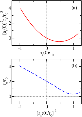
Figure 1: (Color online) Scattering quantities for Gaussian model potential $V_{\rm{g}}$ in the “weakly-interacting” and “strongly-interacting” regimes. (a) The solid line shows the quantity $[a_{s}(0)]^{2}r_{e}/r_{0}^{3}$ as a function of $a_{s}(0)/r_{0}$ (weakly-interacting regime). (b) The dashed line shows the quantity $r_{e}/r_{0}$ as a function of $[a_{s}(0)/r_{0}]^{-1}$ (strongly-interacting regime). Dotted lines are shown to enhance the readability of the graphs.

When $|a_{s}(0)|$ becomes infinitely large, the deviations from universality depend on $r_{e}$ [see Eq. (5)]. The dashed line in Fig. 1(b) shows the effective range $r_{e}/r_{0}$ for the Gaussian model potential as a function of the inverse $s$-wave scattering length $[a_{s}(0)/r_{0}]^{-1}$. The effective range $r_{e}/r_{0}$ is finite and positive as $|a_{s}(0)|\rightarrow\infty$ and varies approximately linearly for small $[a_{s}(0)/r_{0}]^{-1}$ with negative slope.

The higher-order energy-dependence of the $s$-wave scattering length in the “weakly-interacting” and “strongly-interacting” regimes is governed by the volume parameter $V$. The quantity $[a_{s}(0)]^{2}V/r_{0}^{5}$ [see Eq. (6)] goes to zero as $|a_{s}(0)|\rightarrow 0$, and is positive for small $a_{s}(0)/r_{0}<0$ and negative for small $a_{s}(0)/r_{0}>0$. The quantity $V/r_{0}^{3}$ [see Eq. (5)] is finite and negative when the $s$-wave scattering length diverges; $V/r_{0}^{3}$ varies approximately linearly for small $[a_{s}(0)/r_{0}]^{-1}$ with positive slope.

Sections III-V present results for the occupation numbers $n_{{\boldsymbol{\nu}}}$, which are—for inhomogeneous systems—defined by way of the one-body density matrix $\rho({\bf r}_{1}^{\prime},{\bf r}_{1})$ penr56 ; lowd55 ; dubo01 ; blum11 ,

$$\rho({\bf r}^{\prime}_{1}, {\bf r}_{1})=N\times$$ (11)

$$\frac{\int[\psi({\bf r}^{\prime}_{1},{\bf r}_{2},\cdots,{\bf r}_{N})]^{*}\psi({\bf r}_{1},{\bf r}_{2},\cdots,{\bf r}_{N})d^{3}{\bf r}_{2}\cdots d^{3}{\bf r}_{N}}{\int|\psi({\bf r}_{1},\cdots,{\bf r}_{N})|^{2}d^{3}{\bf r}_{1}\cdots d^{3}{\bf r}_{N}}.$$

The one-body density matrix $\rho({\bf r}^{\prime}_{1},{\bf r}_{1})$ can be expanded in terms of a complete orthonormal set,

$$\rho({\bf r}^{\prime}_{1},{\bf r}_{1})=\sum_{{\boldsymbol{\nu}}}n_{{\boldsymbol{\nu}}}\phi^{*}_{{\boldsymbol{\nu}}}({\bf r}_{1})\phi_{{\boldsymbol{\nu}}}({\bf r}^{\prime}_{1}),$$ (12)

where ${\boldsymbol{\nu}}$ collectively denotes the three quantum numbers $\nu\lambda\mu$ needed to uniquely label the functions $\phi_{{\boldsymbol{\nu}}}({\bf r}_{1})$ of the complete orthonormal set. If we use spherical coordinates, $\nu$ is the radial label, $\lambda$ the partial wave label and $\mu$ the corresponding projection number. The quantities $\phi_{{\boldsymbol{\nu}}}({\bf r}_{1})$ and $n_{{\boldsymbol{\nu}}}$ are called natural orbitals and occupation numbers, respectively. Our normalization is chosen such that $\sum_{{\boldsymbol{\nu}}}n_{{\boldsymbol{\nu}}}=N$. The largest occupation number $n_{\boldsymbol{\nu}}$ defines the condensate fraction $N_{0}/N$ of the $N$-boson system, i.e., $N_{0}/N=\mbox{max}(n_{{\boldsymbol{\nu}}}/N)$.

In practice, it is convenient to define partial wave projections $\rho_{\lambda\mu}(r^{\prime}_{1},r_{1})$,

$$\rho_{\lambda\mu}({r}^{\prime}_{1},{r}_{1})=\int Y_{\lambda\mu}^{*}(\hat{r}^{\prime}_{1})\rho({\bf r}^{\prime}_{1}\!,{\bf r}_{1})Y_{\lambda\mu}(\hat{r}_{1})d^{2}\hat{r}^{\prime}_{1}d^{2}\hat{r}_{1},$$ (13)

where $d^{2}\hat{r}_{1}$ and $d^{2}\hat{r}^{\prime}_{1}$ denote angular volume elements. The two-dimensional projections $\rho_{\lambda\mu}(r^{\prime}_{1},r_{1})$ can be diagonalized, yielding the occupation numbers $n_{{\boldsymbol{\nu}}}=n_{\nu\lambda\mu}$ and the radial parts $P_{\nu\lambda}(r_{1})$ of the natural orbitals $\phi_{{\boldsymbol{\nu}}}({\bf r}_{1})$, where $P_{\nu\lambda}(r_{1})$ is defined through $\phi_{{\boldsymbol{\nu}}}({\bf r}_{1})=P_{\nu\lambda}(r_{1})Y_{\lambda\mu}(\hat{r}_{1})$.

III Trapped two-body system

The eigen energies and eigen states of the two-particle Hamiltonian are most easily determined by transforming the Schrödinger equation to center of mass and relative coordinates ${\bf R}_{12}$ and ${\bf r}_{12}$. In these coordinates, the wave function $\psi$ separates into the center of mass wave function $\psi_{QLM}^{\rm{cm}}({\bf R}_{12})$ and the relative wave function $\psi_{qlm}^{\rm{rel}}({\bf r}_{12})$. The two-body energy then reads

$$E_{2}=E_{2}^{\rm{cm}}+E_{2}^{\rm{rel}},$$ (14)

where

$$E_{2}^{\rm{cm}}=(2Q+L+3/2)\hbar\omega$$ (15)

and

$$E_{2}^{\rm{rel}}=(2q+l+3/2)\hbar\omega$$ (16)

with $Q=0,1,\cdots$, $L=0,1,\cdots$ and $l=0,1,\cdots$. For each $L$ ($l$), the center of mass (relative) energy has a $2L+1$ ($2l+1$) degeneracy that is associated with the projection quantum number $M$ ($m$). The allowed values of $q$, and consequently the radial parts of the relative wave function and the relative eigen energies, depend on the functional form of the interaction potential $V_{\rm{tb}}$.

For the energy-dependent zero-range potential $V_{\rm{ps}}$ [see Eq. (3)], the relative wave functions with $l>0$ are not affected by the interaction potential, implying $q=0,1,\cdots$; in this case, the relative wave function coincides with the harmonic oscillator wave function and the two-body energy is independent of the $s$-wave scattering length. For $l=0$, the relative eigen energies are obtained by solving the transcendental equation busc98

$$\frac{\sqrt{2}\Gamma(3/4-E_{2}^{\rm{rel}}/(2\hbar\omega))}{\Gamma(1/4-E_{2}^{\rm{rel}}/(2\hbar\omega))}=\frac{a_{\rm{ho}}}{a_{s}(E_{2}^{\rm{rel}})},$$ (17)

where the energy-dependent $s$-wave scattering length is evaluated at the relative energy of the trapped system, i.e., where we have set $E_{\rm{sc}}^{\rm{rel}}=E_{2}^{\rm{rel}}$ blum02 ; bold02 . Solid lines in Fig. 2 show the relative eigen energies with $l=0$ obtained by solving Eq. (17) with $a_{s}(E_{2}^{\rm{rel}})$ replaced by $a_{s}(0)$ as a function of

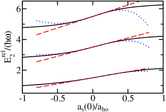
Figure 2: (Color online) Solid lines show the relative energies $E_{2}^{\rm{rel}}$ with $l=0$ for the trapped two-boson system interacting through $V_{\rm{ps}}$, Eq. (17) with $a_{s}(E_{2}^{\rm{rel}})$ replaced by $a_{s}(0)$, as a function of the $s$-wave scattering length $a_{s}(0)/a_{\rm{ho}}$. The dashed and dotted lines show Eq. (III) for $i\leq 1$ and $j=0$, and $i\leq 4$ and $j=0$, respectively.

$a_{s}(0)/a_{\rm{ho}}$. In general, the eigen energies of the trapped two-body system need to be determined self-consistently since $E_{2}^{\rm{rel}}$ appears on the left and right hand sides of Eq. (17) blum02 ; bold02 .

For $|a_{s}(E_{2}^{\rm{rel}})/a_{\rm{ho}}|\ll 1$, we Taylor expand Eq. (17) around the non-interacting relative energies $E_{2,n}^{\rm{ni}}$, where $E_{2,n}^{{\rm ni}}=(2n+3/2)\hbar\omega$ with $n=0,1,\cdots$. Replacing $1/a_{s}(E_{2}^{\rm{rel}})$ by the right hand side of Eq. (5), we find

$$E_{2}^{\rm{rel}}=E_{2,n}^{{\rm ni}}+\sum_{i=1,j=0,j<i}^{i+j\leq 4}d^{(i,j)}_{2,n}\left(\frac{a_{s}(0)}{a_{\rm{ho}}}\right)^{i}\!\!\left(\frac{r_{e}}{a_{\rm{ho}}}\right)^{j}\hbar\omega$$

$$+\cdots.$$ (18)

The next terms are proportional to $[a_{s}(0)]^{5}$, $[a_{s}(0)]^{4}r_{e}$, $[a_{s}(0)]^{3}r_{e}^{2}$ and $[a_{s}(0)]^{2}V$. The coefficients $d^{(i,j)}_{2,n}$ can be compactly written in terms of the quantity $h_{n,p}$,

$$h_{n,p}=H_{n,p}+(-1)^{p}H_{-n-3/2,p},$$ (19)

where $H_{n,p}$ is a generalized harmonic number notation1 . Explicit expressions for the coefficients $d^{(i,j)}_{2,n}$ with $i+j\leq 4$ are reported in Table 1. ​​​

Table 1: Expansion coefficients $d^{(i,j)}_{2,n}$, see Eq. (III), for the weakly-interacting two-boson system with $s$-wave interactions.

$i$	$j$	$d^{(i,j)}_{2,n}$
1	0	$(-1)^{n+1}2^{3/2}/\left[n!\;\Gamma\left(-n-1/2\right)\right]$
2	0	$-4h_{n,1}/\left[n!\;\Gamma\left(-n-1/2\right)\right]^{2}$
3	0	$(-1)^{n+1}2^{3/2}\left(h_{n,2}+3h_{n,1}^{2}\right)/\left[n!\;\Gamma\left(-n-1/2\right)\right]^{3}$
4	0	$-\left(8/3\right)\left(h_{n,3}+6h_{n,2}h_{n,1}+8h_{n,1}^{3}\right)/\left[n!\;\Gamma\left(-n-1/2\right)\right]^{4}$
2	1	$\frac{1}{2}(2n+3/2)d_{2,n}^{(1,0)}$
3	1	$\frac{1}{2}\left(d_{2,n}^{(1,0)}\right)^{2}+(2n+3/2)d_{2,n}^{(2,0)}$

The effective range enters first in combination with the square of the zero-energy scattering length. For the Gaussian potential $V_{\rm{g}}$ considered in Sec. IV, the product $[a_{s}(0)]^{2}r_{e}$ goes to zero as $|a_{s}(0)|\rightarrow 0$ (see solid line in Fig. 1). Dashed and dotted lines in Fig. 2 show Eq. (III) with $j=0$ for $i\leq 1$ and $i\leq 4$, respectively. The Taylor expanded expressions for the ground state with $i\leq 1$ and $i\leq 4$ agree with the exact eigen energy to better than 1% for $-0.22<a_{s}(0)/a_{\rm{ho}}<0.54$ and $-0.67<a_{s}(0)/a_{\rm{ho}}<0.52$, respectively. The accuracy of the Taylor expansion deteriorates more quickly for the excited states. References john09 ; john12 discuss the structure of Eq. (III) with $i+j\leq 3$ for the ground state as well as extensions for $N>2$.

We also expand around the strongly-interacting regime. For $|a_{\rm{ho}}/a_{s}(E_{2}^{\rm{rel}})|\ll 1$, we expand Eq. (17) around the relative energies $E_{2,n}^{\rm{unit}}$ at unitarity, where $E_{2,n}^{{\rm unit}}=(2n+1/2)\hbar\omega$ with $n=0,1,\cdots$. Replacing $1/a_{s}(E_{2}^{\rm{rel}})$ by the right hand side of Eq. (5), we find

$$E_{2}^{\rm{rel}}=E_{2,n}^{{\rm unit}}+\sum_{i=0,j=0}^{i+j\leq 3}\tilde{d}^{(i,j)}_{2,n}\left(\frac{a_{s}(0)}{a_{\rm{ho}}}\right)^{\!\!\!-i}\!\!\!\left(\frac{r_{e}}{a_{\rm{ho}}}\right)^{j}\!\!\!\hbar\omega$$

$$+\frac{1}{8}\left(2n+\frac{1}{2}\right)^{2}\tilde{d}^{(1,0)}_{2,n}\frac{V}{a_{\rm{ho}}^{3}}\hbar\omega+\cdots.$$ (20)

Similarly to the weakly-interacting case, we find it convenient to express the expansion coefficients $\tilde{d}_{2,n}^{(i,j)}$ in terms of the function

$$\tilde{h}_{n,p}=H_{n,p}+(-1)^{p}H_{-n-1/2,p}.$$ (21)

Table 2 shows the expansion coefficients $\tilde{d}_{2,n}^{(i,j)}$ with $i+j\leq 3$. ​​​​​

Table 2: Expansion coefficients $\tilde{d}^{(i,j)}_{2,n}$, see Eq. (III), for the strongly-interacting two-boson system with $s$-wave interactions.

$i$	$j$	$\tilde{d}^{(i,j)}_{2,n}$
0	0	0
1	0	$(-1)^{n+1}2^{3/2}/\left[2\;n!\;\Gamma\left(-n+1/2\right)\right]$
2	0	$-4\tilde{h}_{n,1}/\left[2\;n!\;\Gamma\left(-n+1/2\right)\right]^{2}$
3	0	$(-1)^{n+1}2^{3/2}\left(\tilde{h}_{n,2}+3\tilde{h}_{n,1}^{2}\right)/\left[2\;n!\;\Gamma\left(-n+1/2\right)\right]^{3}$
0	1	$-\frac{1}{2}(2n+1/2)\tilde{d}_{2,n}^{(1,0)}$
1	1	$-\left[\frac{1}{2}\left(\tilde{d}_{2,n}^{(1,0)}\right)^{2}+(2n+1/2)\tilde{d}_{2,n}^{(2,0)}\right]$
2	1	$-\frac{3}{2}\left[\tilde{d}_{2,n}^{(1,0)}\tilde{d}_{2,n}^{(2,0)}+(2n+1/2)\tilde{d}_{2,n}^{(3,0)}\right]$
0	2	$\frac{1}{4}(2n+1/2)\left[\left(\tilde{d}_{2,n}^{(1,0)}\right)^{2}+(2n+1/2)\tilde{d}_{2,n}^{(2,0)}\right]$
1	2	$\frac{1}{4}\bigg{[}\left(\tilde{d}_{2,n}^{(1,0)}\right)^{3}+6(2n+1/2)\tilde{d}_{2,n}^{(1,0)}\tilde{d}_{2,n}^{(2,0)}\qquad$
		$+3\left(2n+1/2\right)^{2}\tilde{d}_{2,n}^{(3,0)}\bigg{]}$
0	3	$-\frac{1}{8}(2n+1/2)\bigg{[}\left(\tilde{d}_{2,n}^{(1,0)}\right)^{3}+3(2n+1/2)\tilde{d}_{2,n}^{(1,0)}\tilde{d}_{2,n}^{(2,0)}\qquad$
		$+\left(2n+1/2\right)^{2}\tilde{d}_{2,n}^{(3,0)}\bigg{]}$

Equation (III) contains contributions that are directly proportional to the inverse scattering length $1/a_{s}(0)$, the effective range $r_{e}$ and the volume term. Which of these terms dominates depends on the interaction potential. Importantly, while the effective range diverges for the Gaussian model potential in the $|a_{s}(0)|\rightarrow 0$ limit, it remains finite in the $|a_{s}(0)|^{-1}\rightarrow 0$ limit [see dashed line in Fig. 1(b)]. The next order terms in Eq. (III) are proportional to $[a_{s}(0)]^{-i}r_{e}^{j}V^{k}$ with $i+j+3k=4$.

Next we discuss the occupation numbers of the two-boson system. The determination of the one-body density matrix for the two-boson system requires that the wave function $\psi$, written above in terms of the center of mass and relative coordinates ${\bf R}_{12}$ and ${\bf r}_{12}$, be transformed to the single particle coordinates ${\bf r}_{1}$ and ${\bf r}_{2}$. In the following, we discuss the occupation numbers associated with the one-body density matrix as a function of the relative two-body energy $E_{2}^{\rm{rel}}$, assuming that the center of mass wave function is in the ground state, i.e., we set $Q=L=M=0$. For two-boson systems in one dimension, the one-body density matrix was calculated as a function of temperature in Ref. ciro01 . Here, we consider the zero temperature limit and restrict ourselves to relative states with $l=0$. The formalism developed, however, can be straighforwardly applied to states with finite $l$, $Q$, $L$ and $M$. As detailed in Appendix B, the one-body density matrix can be evaluated efficiently and with high accuracy by expanding it in terms of single particle harmonic oscillator functions.

We first consider the zero-range pseudopotential $V_{\rm{ps}}$ with $a_{s}(E_{2}^{\rm{rel}})$ replaced by $a_{s}(0)$. Figure 3

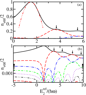
Figure 3: (Color online) Occupation numbers per particle $n_{\nu 00}/N$ of the two-boson system interacting through $V_{\rm{ps}}$ with $a_{s}(E_{2}^{\rm{rel}})$ replaced by $a_{s}(0)$ as a function of the relative two-body energy $E_{2}^{\rm{rel}}$ for $Q=L=M=0$. (a) Solid, dashed and dash-dotted lines show $n_{\nu 00}/2$ for $\nu=0,1$ and $2$, respectively, on a linear scale. The dash-dot-dotted line shows the leading-order depletion, i.e., the first two terms on the right hand side of Eq. (III), near $E_{2}^{\rm{rel}}=3\hbar\omega/2$. (b) Lines show $n_{\nu 00}/2$ for $\nu=0-6$, from top to bottom at $E_{2}^{\rm{rel}}=-5\hbar\omega$, on a log scale. Arrows mark the local maxima of $n_{\nu 00}/2$. Near the non-interacting energies, $(E_{2}^{\rm{rel}}-E_{2,n}^{\rm{rel}})/(\hbar\omega)$ is to a good approximation directly proportional to the $s$-wave scattering length $a_{s}(0)/a_{\rm{ho}}$ [see Eq. (III)], implying that the figure can be read as a “scaled occupation number versus scattering length” plot.

shows the scaled occupation numbers $n_{\nu 00}/2$ for the trapped two-boson system interacting through $V_{\rm{ps}}$ as a function of the relative two-body energy $E_{2}^{\rm{rel}}$. In the non-interacting limit, the ground state with energy $E_{2}^{\rm{rel}}=3\hbar\omega/2$ is characterized by a single natural orbital with projection $\lambda=0$, i.e., the non-interacting two-boson system in the ground state has a condensate fraction $N_{0}/N$ of 1. As the interactions are turned on, i.e., as $a_{s}(0)$ takes on small positive or negative values corresponding to $E_{2}^{\rm{rel}}>3\hbar\omega/2$ and $E_{2}^{\rm{rel}}<3\hbar\omega/2$, respectively, the occupation number associated with the lowest natural orbital depletes. Taylor-expanding the projected one-body density matrix around $E_{2}^{\rm{rel}}=3\hbar\omega/2$ (see Appendix B), we find that the condensate fraction of the ground state of the two-boson system depletes quadratically with $a_{s}(0)$,

$$N_{0}/2=1 -0.420004[a_{s}(0)/a_{\rm{ho}}]^{2}$$

$$-0.373241[a_{s}(0)/a_{\rm{ho}}]^{3}$$

$$+0.406786[a_{s}(0)/a_{\rm{ho}}]^{4}$$

$$+{\cal{O}}([a_{s}(0)/a_{\rm{ho}}]^{5}).$$ (22)

The dash-dot-dotted line in Fig. 3(a) shows the first two terms of Eq. (III), i.e., the leading-order dependence of the depletion on $a_{s}(0)$, in the weakly-interacting regime. The higher-order corrections proportional to $[a_{s}(0)]^{i}$, $i=3$ and 4, are analyzed in Sec. IV.

Figure 3 reveals oscillatory behavior of the scaled occupation numbers $n_{\nu 00}/2$ for $E_{2}^{\rm{rel}}>3\hbar\omega/2$. As the relative energy $E_{2}^{\rm{rel}}$ ($E_{2}^{\rm{rel}}>3\hbar\omega/2$) increases, the occupation numbers go through “near deaths and revivals”, with many of the occupation numbers crossing. When a higher-lying non-interacting state is reached, one more natural orbital with $\lambda=0$ becomes macroscopically occupied. Similar structure is seen for $\lambda>0$ (not shown). For $E_{2}^{\rm{rel}}=7\hbar\omega/2$, e.g., five natural orbitals are occupied. Two of these natural orbitals have $\lambda=0$ with $n_{\nu 00}/2=1/4$ (solid and dashed lines in Fig. 3), while three natural orbitals (from the $2\lambda+1$ degeneracy) have $\lambda=1$ with $n_{\nu 00}/2=1/6$. The largest occupation number per particle $n_{000}/2$ takes on local maxima at the non-interacting energies $E_{2}^{\rm{rel}}=11\hbar\omega/2$ and $19\hbar\omega/2$ as well as at $E_{2}^{\rm{rel}}\approx 3.68\hbar\omega$ and $7.64\hbar\omega$ (see arrows in Fig. 3).

For $E_{2}^{\rm{rel}}<3\hbar\omega/2$, the scaled occupation number $n_{000}/2$ (see solid line in Fig. 3) decreases monotonically with decreasing energy while many other natural orbitals become occupied, including natural orbitals with $\lambda>0$. In the limit of a deeply bound two-body state, the relative two-body wave function becomes infinitely sharply peaked, implying that infinitely many single-particle states are required to describe the deeply-bound two-boson system.

If the energy-dependence of the $s$-wave scattering length is accounted for, the condensate fraction of the two-boson system in the ground state near the non-interacting regime depends not only on $a_{s}(0)$, see Eq. (III), but also on $r_{e}$. We find that the leading-order effective range contribution to the condensate fraction is $-(3/2)\times 0.420004r_{e}[a_{s}(0)]^{3}/a_{\rm{ho}}^{4}$. The factor of $3/2$ arises since the scattering length $a_{s}(0)$ has to be replaced, following Eq. (6), by $[a_{s}(0)]^{2}r_{e}k^{2}/2$, where the relevant energy scale for evaluating $k^{2}$ is $3\hbar\omega/2$ [see Eq. (III) for $n=0$].

IV Weakly-interacting trapped $N$-boson gas

Subsection IV.1 determines the condensate fraction of the lowest gas-like state of the $N$-boson system perturbatively in the weakly-interacting regime, and compares the perturbative predictions with our results for finite-range potentials. Subsection IV.2 parametrizes and quantifies the non-universal corrections revealed through the comparison.

IV.1 Perturbative treatment

We employ the formalism of second quantization and rewrite the $N$-boson Hamiltonian as

$$H=\sum_{{\bf a}}E_{{\bf a}}\hat{a}^{\dagger}_{{\bf a}}\hat{a}_{{\bf a}}+\frac{1}{2}\sum_{{\bf a}{\bf b}{\bf c}{\bf d}}K_{{\bf a}{\bf b}{\bf c}{\bf d}}\hat{a}^{\dagger}_{{\bf a}}\hat{a}^{\dagger}_{{\bf b}}\hat{a}_{{\bf d}}\hat{a}_{{\bf c}},$$ (23)

where

$$K_{{{\bf a}}{{\bf b}}} \;\!\!{}_{{{\bf c}}{{\bf d}}}=$$ (24)

$$\int\!\!\!\!\!\int\!\!\Phi_{{{\bf a}}}^{*}({\bf r}_{1})\Phi_{{{\bf b}}}^{*}({\bf r}_{2})V_{\rm{tb}}({\bf r}_{1}-{\bf r}_{2})\Phi_{{{\bf c}}}({\bf r}_{1})\Phi_{{{\bf d}}}({\bf r}_{2})d^{3}{\bf r}_{1}d^{3}{\bf r}_{2}.$$

Here, the $\Phi_{{{\bf a}}}({\bf r})$ denote the single particle harmonic oscillator wave functions with eigen energy $E_{\bf{a}}$; in spherical coordinates, we have $E_{{\bf a}}=(2n_{a}+l_{a}+3/2)\hbar\omega$. The operators $\hat{a}_{{\bf a}}$ and $\hat{a}_{{\bf a}}^{\dagger}$ obey bosonic commutation relations and respectively annihilate and create a boson in the single particle state $\Phi_{{\bf{a}}}$. We model the interaction $V_{\rm{tb}}$ by the sum $V_{\rm{F}}+V^{\prime}$ (see Sec. II), and employ the counterterms derived in Refs. john09 ; john12 to cure divergencies. Since the $\Phi_{{\bf a}}({\bf r})$ are known, the matrix elements $K_{{\bf a}{\bf b}{\bf c}{\bf d}}$ for this interaction model can be evaluated either analytically or numerically john09 ; john12 . The low-energy Hamiltonian given in Eq. (23) has previously been used to derive perturbative energy expressions up to order $a_{\rm{ho}}^{-3}$ for the harmonically trapped $N$-boson system john12 . In particular, $V_{\rm{F}}$ and $V^{\prime}$ were treated at the level of third- and first-order perturbation theory. Comparison with energies for systems with finite-range interactions validated the formalism and showed that the derived perturbative energy expressions, which depend on $a_{s}(0)$ and $r_{e}$, provide an excellent description in the weakly-interacting regime john12 .

To determine the condensate fraction, we construct the matrix $\langle\hat{a}_{\bf p}^{\dagger}\hat{a}_{\bf q}\rangle$, where ${\bf p}$ and ${\bf q}$ run over all possible single-particle state labels. The expectation value $\langle\hat{a}_{\bf p}^{\dagger}\hat{a}_{\bf q}\rangle$,

$$\langle\hat{a}_{\bf p}^{\dagger}\hat{a}_{\bf q}\rangle=\frac{\langle\psi_{\bf{0}}^{(k)}|\hat{a}_{\bf p}^{\dagger}\hat{a}_{\bf q}|\psi_{\bf{0}}^{(k)}\rangle}{\langle\psi_{\bf{0}}^{(k)}|\psi_{\bf{0}}^{(k)}\rangle},$$ (25)

is calculated with respect to the many-body ground state wave function $\psi_{\bf{0}}^{(k)}$, determined within $k$^th-order perturbation theory. The ground state wave function $\psi_{\bf{0}}^{(k)}$ is expressed as a superposition of the unperturbed many-body wave functions $\psi_{\bf{j}}^{(0)}$,

$$|\psi_{\bf{0}}^{(k)}\rangle=\sum_{\bf j}b_{\bf j}^{(k)}|\psi_{\bf j}^{(0)}\rangle,$$ (26)

where the expansion coefficients $b_{\bf j}^{(k)}$ are determined by the matrix elements $K_{{\bf{a}}{\bf{b}}{\bf{c}}{\bf{d}}}$. The subscript ${\bf j}$ collectively labels the non-interacting or unperturbed many-body states (in particular, ${\bf{0}}$ labels the ground state). Once the matrix $\langle\hat{a}_{\bf{p}}^{\dagger}\hat{a}_{\bf{q}}\rangle$ is constructed, we diagonalize it analytically (see Appendix A). Up to order $a_{\rm{ho}}^{-3}$, i.e., treating the second-order perturbation theory wave function, we find

$$N_{0}/N=1 -0.420004(N-1)\left[\frac{a_{s}(0)}{a_{\rm{ho}}}\right]^{2}$$

$$+\big{[}-0.373241(N-1)$$

$$\quad\;\;+0.439464(N-1)(N-2)\big{]}\left[\frac{a_{s}(0)}{a_{\rm{ho}}}\right]^{3}$$

$$+\cdots.$$ (27)

The prefactors are discussed in the context of Table 3. We interpret the terms proportional to $(N-1)$ and $(N-1)(N-2)$ as being due to two-body and three-body scattering processes, respectively. In Eq. (IV.1), the terms proportional to $[a_{s}(0)]^{2}$ and $[a_{s}(0)]^{3}$ arise when treating the potential $V_{\rm{F}}$, together with the appropriate counterterm, in first- and second-order perturbation theory. Treating $V_{\rm{F}}$ in third-order perturbation theory (not pursued here), three terms proportional to $[a_{s}(0)]^{4}$ that contain the factors $(N-1)$, $(N-1)(N-2)$ and $(N-1)(N-2)(N-3)$, respectively, are expected to arise.

The potential $V^{\prime}$ does not, in first-order perturbation theory, give rise to a two-body term proportional to $r_{e}[a_{s}(0)]^{2}/a_{\rm{HO}}^{3}$. This result agrees with that obtained by Taylor-expanding the full two-body density matrix and determining its largest eigen value (see last paragraph of Sec. III). No three-body term arises at order $r_{e}[a_{s}(0)]^{3}$. Since the leading-order effective range dependence is of order $a_{\rm{ho}}^{-4}$, it is not included in Eq. (IV.1).

To assess the applicability of our perturbatively derived result, Eq. (IV.1), we calculate the condensate fraction for small $N$-boson systems interacting through the Gaussian model potential $V_{\rm{g}}$, Eq. (10), with small $|a_{s}(0)|/a_{\rm{ho}}$. For $N=2$, we solve the relative Schrödinger equation using standard B-spline techniques. For $N=3$ and $4$, we use the stochastic variational approach cgbook ; sore05 , which expands the relative eigen functions in terms of a set of fully symmetrized basis functions whose widths are chosen semi-stochastically. The widths are optimized by minimizing the ground state energy. The optimized ground state wave function is then used to construct the projected one-body density matrix $\rho_{00}(r^{\prime}_{1},r_{1})$ on a grid in the $r^{\prime}_{1}$ and $r_{1}$ coordinates. The projected one-body density matrix is diagonalized numerically to find the natural orbitals and their occupation numbers. The resulting condensate fraction for $N=3$ has an estimated numerical error of order $10^{-7}$ or smaller for the parameter combinations considered. The numerical error is due to the facts that (i) we use a finite basis set, (ii) we construct $\rho_{00}(r^{\prime}_{1},r_{1})$ on a grid with finite grid spacings, and (iii) our grid terminates at finite $r^{\prime}_{1}$ and $r_{1}$ values. For $N=3$, we use around 120 basis functions and 625 linearly spaced grid points in $r^{\prime}_{1}$ and $r_{1}$ between $r_{0}/2$ and $5.5a_{\rm{ho}}$.

Squares and circles in Fig. 4(a) show the condensate fraction $N_{0}/N$ for the $N=2$ and $N=3$ systems interacting through $V_{\rm{g}}$ with $r_{0}=0.01a_{\rm{ho}}$ as a function of the zero-energy $s$-wave scattering length $a_{s}(0)$.

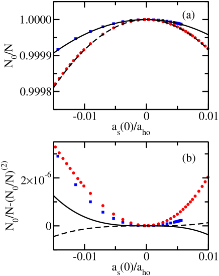
Figure 4: (Color online) Condensate fraction $N_{0}/N$ of the weakly-interacting $N$-boson system as a function of $a_{s}(0)/a_{\rm{ho}}$. (a) Squares and circles show the condensate fraction for $N=2$ and $3$ bosons interacting through the shape-dependent Gaussian model potential $V_{\rm{g}}$ with $r_{0}=0.01a_{\rm{ho}}$. Solid and dashed lines show Eq. (IV.1) for $N=2$ and $3$, respectively. (b) Squares and circles show the quantity $N_{0}/N-(N_{0}/N)^{(2)}$ for $N=2$ and 3 using the same data as in panel (a). Solid and dashed lines show the $[a_{s}(0)/a_{\rm{ho}}]^{3}$ term of Eq. (IV.1) for $N=2$ and $3$.

For comparison, solid and dashed lines show our perturbative results up to order $a_{\rm{ho}}^{-3}$. It can be seen that the numerically determined condensate depletions for the finite-range interaction potential change approximatically quadratically with the scattering length. To investigate the correction proportional to $[a_{s}(0)/a_{\rm{ho}}]^{3}$, squares and circles in Fig. 4(b) show the quantity $N_{0}/N-(N_{0}/N)^{(2)}$, where $(N_{0}/N)^{(2)}=1-(N-1)0.420004[a_{s}(0)/a_{\rm{ho}}]^{2}$, for $N=2$ and 3 [the data for $N_{0}/N$ are the same as those shown in Fig. 4(a)]. For comparison, the solid and dashed lines show the perturbatively predicted $[a_{s}(0)/a_{\rm{ho}}]^{3}$ dependence for $N=2$ and $3$. It can be seen that the perturbative prediction does not provide a good description of the sub-leading dependence of the depletion. Similar behavior is observed for $N=4$ (not shown). We find that neither the inclusion of the $r_{e}[a_{s}(0)]^{3}$ nor of the $[a_{s}(0)]^{4}$ terms can explain the discrepancy. As shown in the next subsection, the discrepancy displayed in Fig. 4(b) is due to non-universal contributions.

IV.2 Non-universal contributions

To better connect the results obtained by applying perturbation theory to the low-energy Hamiltonian, Eq. (23) with $V_{\rm{tb}}=V_{\rm{F}}+V^{\prime}$, with the results for the Hamiltonian with finite-range interactions, we first consider the two-body system. Noting that the perturbative results for the condensate fraction agree with the results obtained by Taylor-expanding the exact one-body density matrix for the two-body system with regularized zero-range interaction [i.e., noting that Eq. (IV.1) agrees with Eq. (III) for $N=2$ and the orders considered], we compare the one-body density matrix $\rho({\bf{r}}^{\prime}_{1},{\bf{r}}_{1})$ for the two-body system interacting through $V_{\rm{ps}}$ with the one-body density matrix $\rho_{\rm{fr}}({\bf{r}}^{\prime}_{1},{\bf{r}}_{1})$ for the two-body system interacting through a finite-range potential.

Since the regularized zero-range potential reproduces the relative two-body energy of systems with finite-range interactions with high accuracy bold02 ; blum02 , we assume that the relative two-body energies $E_{2}^{\rm{rel}}$ agree for the two interaction models. We denote the normalized relative wave function of the energetically lowest-lying gas-like state for the finite-range potential by $\psi^{\rm{rel,fr}}({\bf{r}}_{12})$ and that for the regularized zero-range model potential by $\psi_{q00}^{\rm{rel}}({\bf{r}}_{12})$ [see Eq. (54)]. It is instructive to write $\psi^{\rm{rel,fr}}$ as

$$\psi^{\rm{rel,fr}}({\bf{r}}_{12})=\psi_{q00}^{\rm{rel}}({\bf{r}}_{12})+\delta\psi({\bf{r}}_{12}).$$ (28)

Inserting Eq. (28) into $\rho_{\rm{fr}}({\bf{r}}^{\prime}_{1},{\bf{r}}_{1})$ and assuming the absence of center of mass excitations, we find

$$\rho_{\rm{fr}}({\bf{r}}^{\prime}_{1},{\bf{r}}_{1})\approx\rho({\bf{r}}^{\prime}_{1},{\bf{r}}_{1})+2\delta\rho({\bf{r}}^{\prime}_{1},{\bf{r}}_{1}),$$ (29)

where $\rho({\bf{r}}^{\prime}_{1},{\bf{r}}_{1})$ is given in Eqs. (B) and (68), and

$$\delta\rho({\bf{r}}^{\prime}_{1} ,{\bf{r}}_{1})=$$ (30)

$$\int[\psi^{\rm{cm}}_{000}({\bf{R}}^{\prime}_{12})\delta\psi({\bf{r}}^{\prime}_{12})]^{*}\psi^{\rm{cm}}_{000}({\bf{R}}_{12})\psi_{q00}^{\rm{rel}}({\bf{r}}_{12})d^{3}{\bf{r}}_{2}$$

$$+\int[\psi^{\rm{cm}}_{000}({\bf{R}}^{\prime}_{12})\psi_{q00}^{\rm{rel}}({\bf{r}}^{\prime}_{12})]^{*}\psi^{\rm{cm}}_{000}({\bf{R}}_{12})\delta\psi({\bf{r}}_{12})d^{3}{\bf{r}}_{2}$$

with ${\bf{r}}^{\prime}_{12}={\bf{r}}_{1}^{\prime}-{\bf{r}}_{2}$ and ${\bf{R}}^{\prime}_{12}=({\bf{r}}_{1}^{\prime}+{\bf{r}}_{2})/2$; ${\bf{r}}_{12}$ and ${\bf{R}}_{12}$ are defined in Sec. II. In writing Eq. (29), the term proportional to $|\delta\psi|^{2}$ has been neglected.

To determine the condensate fraction, we expand $\delta\rho({\bf{r}}^{\prime}_{1},{\bf{r}}_{1})$ in terms of non-interacting single particle harmonic oscillator functions; this approach is analogous to that discussed in detail in Appendix B for $\rho({\bf{r}}^{\prime}_{1},{\bf{r}}_{1})$. A fairly straightforward analysis shows that the main correction to the condensate fraction arises from the $((0,0,0),(0,0,0))$ element of $\delta\rho({\bf{r}}^{\prime}_{1},{\bf{r}}_{1})$. It follows that the largest occupation number $n_{000}^{\rm{fr}}$ for the finite-range potential can be written as

$$\frac{n_{000}^{\rm{fr}}}{2}\approx\frac{n_{000}}{2}+\delta c_{00},$$ (31)

where

$$\delta c_{00}=\sum_{i=0}^{\infty}2^{-2i}(C_{i}^{*}D_{i}+C_{i}D_{i}^{*}).$$ (32)

In Eq. (31), $n_{000}/2=N_{0}/2$ denotes the condensate fraction of the two-body system interacting through the regularized zero-range potential [see Eq. (III)]. The coefficients $C_{i}$ are defined in Eq. (60) and the $D_{i}$ denote the overlaps between the non-interacting harmonic oscillator functions and $\delta\psi$,

$$D_{i}=\int[\psi_{i00}^{\rm{rel,ni}}({\bf{r}}_{12})]^{*}\delta\psi({\bf{r}}_{12})d^{3}{\bf{r}}_{12}.$$ (33)

Realizing that the $i=0$ terms in Eq. (32) dominate and using the leading-order behavior of $C_{0}$, i.e., $C_{0}\approx 1$ [see Eqs. (71) and (72)], we find

$$\delta c_{00}\approx 2{\mbox{Re}}(D_{0}).$$ (34)

For the finite-range potentials considered in this paper, we find that Eqs. (32) and (34) deviate by less than 0.2 %. In the following, we refer to $D_{0}$ as the “non-universal two-body parameter”.

Figure 5 illustrates the behavior of the integrand that determines the non-universal two-body parameter $D_{0}$ for two different two-body energies, i.e., for $E_{2}^{\rm{rel}}=1.498\hbar\omega$ [negative $a_{s}(0)$] and $E_{2}^{\rm{rel}}=1.502\hbar\omega$ [positive $a_{s}(0)$], for the Gaussian model potential with $r_{0}=0.01a_{\rm{ho}}$. In particular, Fig. 5(a) shows the product $(\psi_{000}^{\rm{rel,ni}})^{*}\delta\psi$ and Fig. 5(b) the ratio $\psi^{\rm{rel,fr}}/\psi^{\rm{rel}}_{q00}$. Figure 5 reflects the presence of the two characteristic length scales of the problem. The behavior in the small $r_{12}$ region, shown in the insets of Figs. 5(a) and 5(b), is governed by the details of the two-body interaction potential. Near $r_{12}\approx 5r_{0}$, the behavior of $(\psi_{000}^{\rm{rel,ni}})^{*}\delta\psi$ and $\psi^{\rm{rel,fr}}/\psi^{\rm{rel}}_{q00}$ changes notably. For $r_{12}\gtrsim 5r_{0}$,

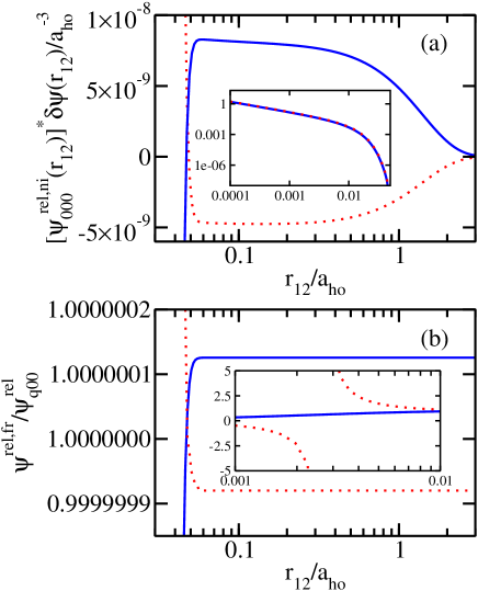
Figure 5: (Color online) Analysis of the integrand that determines the non-universal parameter $D_{0}$ [see Eq. (33)] for the finite-range model potential $V_{\rm{g}}$ with $r_{0}=0.01a_{\rm{ho}}$ for two different relative two-body energies. The solid and dotted lines correspond to $E_{2}^{\rm{rel}}=1.498\hbar\omega$ and $E_{2}^{\rm{rel}}=1.502\hbar\omega$, respectively. Panel (a) shows the integrand $[\psi_{000}^{\rm{rel,ni}}({\bf{r}}_{12})]^{*}\delta\psi({\bf{r}}_{12})$ in the large $r_{12}$ region, i.e., for $r_{12}\in[0.03a_{\rm{ho}},3a_{\rm{ho}}]$ (log-linear scale), while the inset shows the absolute value of the integrand $|[\psi_{000}^{\rm{rel,ni}}({\bf{r}}_{12})]^{*}\delta\psi({\bf{r}}_{12})|$ in the small $r_{12}$ region (log-log scale). Panel (b) and the inset of (b) show the ratio $\psi^{\rm{rel,fr}}/\psi_{q00}^{\rm{rel}}$ in the large and small $r_{12}$ regions, respectively (log-linear scale).

the ratio $\psi^{\rm{rel,fr}}/\psi_{q00}^{\rm{rel}}$ approaches a constant that is slightly larger (smaller) than 1 for negative (positive) $a_{s}(0)$. The small deviations of the ratios from one are a consequence of the fact that the wave functions of the trapped system are normalized to one. Since the wave functions for the finite range interaction potential deviate from those for the zero-range interaction potential in the small $r_{12}$ region, the ratio $\psi^{\rm{rel,fr}}/\psi_{q00}^{\rm{rel}}$ needs—in general—to differ from one in the large $r_{12}$ region. The “divergence” of the ratio $\psi^{\rm{rel,fr}}/\psi_{q00}^{\rm{rel}}$ near $r_{12}=0.002a_{\rm{ho}}$ for $a_{s}(0)>0$ [see dotted line in the inset of Fig. 5(b)] reflects the fact that the zero-range potential supports a deeply-bound negative energy state, which introduces a node at small $r_{12}$ in the wave function that describes the energetically lowest-lying gas-like state. A corresponding bound-state is not supported by the purely repulsive Gaussian model potential, leading to an infinite ratio $\psi^{\rm{rel,fr}}/\psi_{q00}^{\rm{rel}}$ at the node of $\psi_{q00}^{\rm{rel}}$.

The non-universal two-body parameter $D_{0}$ is the trap analog of the two-body scattering quantity $u_{0}$ introduced by Tan [see Eq. (114a) of Ref. tan08 ]. It is important to note, however, that $D_{0}$ depends on the wave function difference for all $r_{12}$ and on the non-interacting harmonic oscillator ground state wave function while the $u_{0}$ defined by Tan depends only on the wave function difference in the small $r_{12}$ region, i.e., out to a few times $r_{0}$. Indeed, we find that the contribution to $D_{0}$ that accumulates in the inner region ($r_{12}\lesssim 10r_{0}$) can be of comparable magnitude to the contribution that accumulates in the outer region ($r_{12}\gtrsim 10r_{0}$).

Since the dependence of the condensate fraction on the quantity $D_{0}$ arises at the two-body level, the $D_{0}$ term needs to be multiplied by $N-1$ for systems with $N>2$. Figure 6 compares the condensate fractions for the $N=2$ and $3$ systems interacting through the finite-range Gaussian model potential $V_{\rm{g}}$ with the predicted behavior for the condensate fraction.

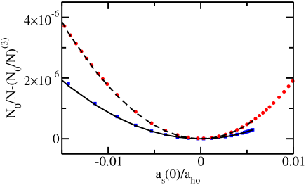
Figure 6: (Color online) Squares and circles show the residual $N_{0}/N-(N/N_{0})^{(3)}$ for $N=2$ and $3$ as a function of $a_{s}(0)$ for the Gaussian model interaction $V_{\rm{g}}$ with $r_{0}=0.01a_{\rm{ho}}$. Solid and dashed lines show the quantity $(N-1)\delta c_{00}$ for $N=2$ and $3$, respectively notation2 .

Specifically, squares and circles show the difference $N_{0}/N-(N_{0}/N)^{(3)}$ for $N=2$ and $3$ between the numerically determined condensate fraction $N/N_{0}$ and the perturbative result $(N_{0}/N)^{(3)}$, which includes all terms on the right hand side of Eq. (IV.1) up to order $a_{\rm{ho}}^{-3}$. According to our discussion above, we expect that the residuals are well approximated by $(N-1)\delta c_{00}$ (shown by solid and dashed lines in Fig. 6). Indeed, Fig. 6 shows that the residuals for $N=2$ and $3$ are well described by the non-universal corrections. We find similar results for $N=4$ (not shown). Our calculations demonstrate that two Hamiltonians that are characterized by the same energy give rise to condensate fractions that differ. Related findings have previously been discussed in Refs. coes70 ; furn02 ; tan08 . The leading order difference between the condensate fractions for the harmonically trapped few-boson systems described by the two Hamiltonians can be parameterized by the non-universal two-body parameter $D_{0}$, a parameter not needed to match the energies of the two Hamiltonians.

V Three trapped bosons at unitarity

The previous section discussed the condensate fraction of weakly-interacting trapped $N$-boson systems, which can be expressed in terms of $a_{s}(0)$, $r_{e}$ and a non-universal two-body correction parametrized through $D_{0}$. It is well known that the properties of the three-boson system not only depend on two-body parameters, but also on a three-body parameter efim71 ; efim73 ; braa06 . In the weakly-interacting regime, however, the dependence on the three-body parameter appears at higher order than considered in Sec. IV. In the strongly-interacting regime, in contrast, the dependence on the three-body parameter is generally quite pronounced.

At unitarity, i.e., for diverging $a_{s}(0)$, the trapped three-boson system with zero-range $s$-wave interactions supports two distinct classes of eigen states: (i) universal states whose properties are fully governed by the two-body scattering parameters, and (ii) non-universal states whose properties depend, in addition to the two-body scattering parameters, on a three-body parameter. In the following, we determine the occupation numbers for the non-universal three-boson states in a trap at unitarity as a function of the three-body parameter. The momentum distribution of Efimov trimers in free-space was discussed in Ref. wern11 .

The three-boson wave function $\psi({\bf{r}}_{1},{\bf{r}}_{2},{\bf{r}}_{3})$ with relative orbital angular momentum $l=0$ for zero-range interactions with diverging $s$-wave scattering length $a_{s}(0)$, and vanishing $r_{e}$ and $V$, under external isotropic harmonic confinement can be written as jons02 ; wern06a

$$\psi({\bf{r}}_{1},{\bf{r}}_{2},{\bf{r}}_{3})={\cal{S}}\left[R^{-5/2}F(R)\varphi(\alpha)\psi_{QLM}^{\rm{cm}}({\bf{R}}_{123})\right].$$ (35)

Here, $R$ denotes the hyperradius and $\alpha$ the hyperangle, $R^{2}=r_{12}^{2}/2+2r_{12,3}^{2}/3$ and $\tan\alpha=\sqrt{3}r_{12}/(2r_{12,3})$ with $r_{12}=|{\bf{r}}_{1}-{\bf{r}}_{2}|$ and $r_{12,3}=|({\bf{r}}_{1}+{\bf{r}}_{2})/2-{\bf{r}}_{3}|$. In Eq. (35), $\psi_{QLM}^{\rm{cm}}({\bf{R}}_{123})$ denotes the harmonic oscillator wave function in the center of mass coordinate ${\bf{R}}_{123}$, ${\bf{R}}_{123}=({\bf{r}}_{1}+{\bf{r}}_{2}+{\bf{r}}_{3})/3$; as in Sec. III, we assume that the center of mass wave function is in the ground state, i.e., we set $Q=L=M=0$. The operator ${\cal{S}}$ ensures that the three-boson wave function is symmetric under the exchange of any of the three boson pairs, ${\cal{S}}=1+P_{12}+P_{23}+P_{31}+P_{12}P_{23}+P_{12}P_{31}$, where $P_{jk}$ is the operator that exchanges particles $j$ and $k$. The hyperangular wave function $\varphi(\alpha)$ takes the form $\varphi(\alpha)=\sin[(\alpha-\pi/2)s_{0}]/\sin(2\alpha)$, where $s_{0}$ equals $1.00624\imath$ efim71 ; efim73 ; braa06 . The fact that the separation constant $s_{0}$, which arises when solving the hyperangular Schrödinger equation, is imaginary is unique to the $l=0$ channel and tightly linked to the fact that a three-body parameter is needed.

The hyperradial wave function $F(R)$ can be conveniently expressed in terms of the Whittaker function $W$ wern06a , i.e., $F(R)=R^{-1/2}W_{E^{\rm{rel}}_{3}/2,s_{0}/2}(R^{2}/a_{\rm{ho}}^{2})$. The relative three-body energy $E^{\rm{rel}}_{3}$ is related to the three-body or Efimov phase $\theta$ through jons02

$$\theta=\mbox{arg}\left(\frac{\Gamma\left(\frac{1}{2}-\frac{E^{\rm{rel}}_{3}}{2\hbar\omega}+\frac{s_{0}}{2}\right)}{\Gamma(1+s_{0})}\right).$$ (36)

The physical meaning of $\theta$ becomes clear when looking at the small $R/a_{\rm{ho}}$ behavior of $F(R)$, $F(R)\rightarrow\sqrt{R}\sin(\mbox{Im}(s_{0})\ln(R/a_{\rm{ho}})+\theta)$. This expression shows that the three-body phase determines what happens when three particles come close together. The small $R/a_{\rm{ho}}$ behavior can be thought of as being imposed by a short-range three-body force or a boundary condition of the hyperradial wave function in the $R/a_{\rm{ho}}\rightarrow 0$ limit braa06 .

To determine the occupation numbers of the non-universal three-boson states as a function of $E^{\rm{rel}}_{3}$, we sample the density $|\psi({\bf{r}}_{1},{\bf{r}}_{2},{\bf{r}}_{3})|^{2}$ using Metropolis sampling. As discussed in Ref. blum11 , this approach introduces a statistical error that can be reduced by performing longer random walks. Throughout our random walk, we sample the projected one-body density matrix $\rho_{00}(r^{\prime}_{1},r_{1})$. Diagonalizing $\rho_{00}(r^{\prime}_{1},r_{1})$ at the end of a run yields the occupation numbers.

Figure 7 shows the two largest occupation numbers per particle $n_{\nu 00}/3$ as a function of $E_{3}^{\rm{rel}}$.

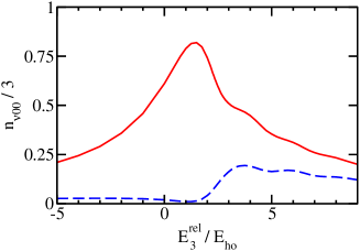
Figure 7: (Color online) Occupation numbers per particle $n_{\nu 00}/N$ [$\nu=0$ (solid line) and $\nu=1$ (dashed line)] for the non-universal $l=0$ state of the three-boson system at unitarity as a function of the relative three-body energy $E^{\rm{rel}}_{3}$ in units of the oscillator energy $E_{\rm ho}$, $E_{\rm ho}=\hbar\omega$; the three-body energy can be converted to the three-body parameter via Eq. (36).

It can be seen that the occupation numbers of the non-universal state depend quite strongly on the relative three-body energy or, equivalently, the three-body phase $\theta$. The maximum of the lowest occupation number per particle $n_{000}/3$ is $0.82$ and occurs at $E_{3}^{\rm{rel}}=3\hbar\omega/2$; the occupation number per particle $n_{100}/3$ is minimal at this energy. Interestingly, the occupation numbers show oscillations (or “shoulders”) similar to those discussed in the context of Fig. 3 for the two-body system. In Figure 3, we change the relative two-body energy, which is related to the $s$-wave scattering length through Eq. (17). In Fig. 7, we change the relative three-body energy, which is related to the three-body phase through Eq. (36). For both the two- and three-body systems, Eqs. (17) and (36) can be related to the short-range boundary condition of the respective radial or hyperradial part of the relative wave function.

For comparison, we also calculated the largest occupation number per particle of the projected one-body density matrix $\rho_{00}(r^{\prime}_{1},r_{1})$ for selected universal three-boson states (see Ref. wern06a for the relevant wave functions). The largest occupation number per particle of the energetically lowest-lying universal three-boson state with $l=0$ and $E_{3}^{\rm{rel}}=4.465\hbar\omega$ at unitarity is $n_{000}/3=0.295$. The largest occupation numbers per particle of the energetically lowest lying states with $l=1$ and $l=2$ at unitarity are $n_{000}/3=0.199$ and $0.421$, respectively. For these states, the energies are $E_{3}^{\rm{rel}}=2.864\hbar\omega$ and $E_{3}^{\rm{rel}}=2.823\hbar\omega$, respectively. For the universal states considered, the largest occupation number $n_{000}$ is notably smaller than $N$.

VI Conclusions

We have determined and interpreted the occupation numbers of few-boson systems under isotropic harmonic confinement. In the weakly-interacting regime, our analysis is based on a low-energy Hamiltonian—characterized by the $s$-wave scattering length $a_{s}(0)$ and the effective range $r_{e}$—that has previously been proven to correctly describe the energy of few-boson systems up to order $a_{\rm{ho}}^{-3}$ john12 . The present paper shows that this low-energy Hamiltonian correctly describes the leading order depletion of harmonically trapped few-boson systems but that it does not fully capture the corrections to the leading order depletion.

Our final expression for the condensate fraction reads

$$N_{0}/N=1 -0.420004(N-1)\left[\frac{a_{s}(0)}{a_{\rm{ho}}}\right]^{2}$$

$$+\big{[}-0.373241(N-1)$$

$$\quad\;\;+0.439464(N-1)(N-2)\big{]}\left[\frac{a_{s}(0)}{a_{\rm{ho}}}\right]^{3}$$

$$+\big{[}0.406786(N-1)+\gamma_{3}^{(4)}(N-1)(N-2)$$

$$\quad\;\;+\gamma_{4}^{(4)}(N-1)(N-2)(N-3)\big{]}\left[\frac{a_{s}(0)}{a_{\rm{ho}}}\right]^{4}$$

$$+2(N-1)\mbox{Re}(D_{0})$$

$$-(3/2)\times 0.420004(N-1)\frac{r_{e}[a_{s}(0)]^{3}}{a_{\rm{ho}}^{4}}$$

$$+\cdots,$$ (37)

where the non-universal two-body parameter $D_{0}$ is defined in Eq. (33). The coefficients $\gamma_{3}^{(4)}$ and $\gamma_{4}^{(4)}$ arise when treating $V_{\rm{F}}$ in third-order perturbation theory; the determination of their numerical values is beyond the scope of this paper. We have confirmed the expression for the condensate fraction, Eq. (VI), through comparison with numerical results for a few-body Hamiltonian with finite-range two-body potentials. Our work demonstrates that the occupation numbers are not fully determined by the parameters of the “usual” effective range expansion, but rather depend on an additional property of the two-body wave function (i.e., non-universal physics). A similar result is expected to hold for the momentum distribution. Our findings are not only of importance for cold atomic Bose gases but also for nuclear systems, for which the use of low-energy Hamiltonians has become increasingly more popular during the past decade or so epelbaum .

We have also considered the strongly-interacting regime. Our results show that the occupation numbers for non-universal states of the three-boson system under isotropic harmonic confinement depend strongly on the three-body parameter. This finding suggests that the occupation numbers and momentum distribution of strongly-interacting Bose gases at unitarity may depend on three-body physics. In view of recent experimental work papp08 ; navo10 ; wild12 , it would be interesting to extend the treatments of Refs. song09 ; lee10 , which predict—accounting only for two-body physics—that three-dimensional Bose gases at unitarity fermionize. In particular, it would be interesting to determine how, if at all, this fermionization picture changes if three-body physics is accounted for.

VII Acknowledgement

Support by the NSF through grant PHY-0855332, and fruitful discussions with P. Johnson and E. Tiesinga on the renormalized perturbation theory framework are gratefully acknowledged.

Appendix A Perturbative treatment and diagonalization of one-body density matrix

This appendix provides details regarding the perturbative treatment of the condensate fraction of the $N$-boson system and the diagonalization of the associated matrix.

We start with the Hamiltonian $H$ given by Eq. (23). We first neglect the effective range dependent potential $V^{\prime}$, i.e., we consider only the bare Fermi pseudopotential $V_{\rm{F}}$, Eq. (8), and the counterterm $W$ used to cure divergencies john09 ; john12 . The matrix elements $K_{\mathbf{abcd}}$ can then be written as

$$K_{\mathbf{abcd}}=F_{\mathbf{abcd}}\left[\frac{a_{s}(0)}{a_{\rm{ho}}}+\nu\left(\frac{a_{s}(0)}{a_{\rm{ho}}}\right)^{2}\right]\hbar\omega,$$ (38)

where

$$F_{\mathbf{a}\mathbf{b}\mathbf{c}\mathbf{d}}=4\pi a_{\rm{ho}}^{3}\int\Phi_{\mathbf{a}}^{*}(\mathbf{r}_{1})\Phi_{\mathbf{b}}^{*}(\mathbf{r}_{1})\Phi_{\mathbf{c}}(\mathbf{r}_{1})\Phi_{\mathbf{d}}(\mathbf{r}_{1})d^{3}\mathbf{r}_{1}$$ (39)

and

$$\nu=\sqrt{\frac{2}{\pi}}(1-\ln 2)+\sqrt{\frac{\pi}{2}}\beta_{2}^{(2)}.$$ (40)

The coefficient $\beta_{2}^{(2)}$ was calculated in Ref. john12 and is listed in Table 3. It diverges and cures the divergencies that arise when treating $V_{\rm{F}}$ in second-order perturbation theory.

The matrix $\langle\hat{a}_{\mathbf{p}}^{\dagger}\hat{a}_{\mathbf{q}}\rangle$ is evaluated by substituting Eq. (26) into Eq. (25). In order to get the matrix elements up to order $a_{\rm{ho}}^{-3}$, we need to employ second order perturbation theory. The expansion coefficients $b_{{\bf j}}^{(2)}$ of the non-normalized second-order wave function $\psi_{\bf{0}}^{(2)}$ read

$$b_{{\bf{0}}}^{(2)}=1$$ (41)

and

$$b_{{\bf j}}^{(2)}= -\frac{\langle\psi_{{\bf j}}^{(0)}|V_{\rm{F}}+W|\psi_{\bf{0}}^{(0)}\rangle}{E_{{\bf j}}^{(0)}-E_{\bf{0}}^{(0)}}$$

$$+\sum_{{\bf j}^{\prime}\neq{\bf{0}}}\frac{\langle\psi_{{\bf j}}^{(0)}|V_{\rm{F}}+W|\psi_{{\bf j}^{\prime}}^{(0)}\rangle\langle\psi_{{\bf j}^{\prime}}^{(0)}|V_{\rm{F}}+W|\psi_{\bf{0}}^{(0)}\rangle}{(E_{{\bf j}}^{(0)}-E_{\bf{0}}^{(0)})(E_{{\bf j}^{\prime}}^{(0)}-E_{\bf{0}}^{(0)})}$$

$$-\frac{\langle\psi_{{\bf j}}^{(0)}|V_{\rm{F}}+W|\psi_{\bf{0}}^{(0)}\rangle\langle\psi_{\bf{0}}^{(0)}|V_{\rm{F}}+W|\psi_{\bf{0}}^{(0)}\rangle}{(E_{{\bf j}}^{(0)}-E_{\bf{0}}^{(0)})^{2}}$$ (42)

for ${\bf{j}}$ not equal to the ground state labeled by ${\bf{0}}$. In the denominators appearing in Eq. (A), the $E_{\bf{j}}^{(0)}$ denote the unperturbed eigen energies corresponding to the ${\bf{j}}$’s unperturbed eigen state. The numerators are conveniently expressed in terms of the matrix elements $F_{\mathbf{a}\mathbf{b}\mathbf{c}\mathbf{d}}$.

The indices $\mathbf{p}$ and $\mathbf{q}$ of $\langle\hat{a}_{\mathbf{p}}^{\dagger}\hat{a}_{\mathbf{q}}\rangle$ run over all possible single particle state labels. We employ spherical coordinates and write ${\bf{p}}=(n_{1}^{\prime},l_{1}^{\prime},m_{1}^{\prime})$ and ${\bf{q}}=(n_{1},l_{1},m_{1})$. We find that the matrix is block diagonal, i.e., $\langle\hat{a}_{n_{1}^{\prime}l_{1}^{\prime}m_{1}^{\prime}}^{\dagger}\hat{a}_{n_{1}l_{1}m_{1}}\rangle=0$ for $l_{1}^{\prime}\neq l_{1}$ or $m_{1}^{\prime}\neq m_{1}$. In the following, we consider the submatrix with $l_{1}^{\prime}=l_{1}=m_{1}^{\prime}=m_{1}=0$. We denote the matrix elements by $c_{n_{1}^{\prime}n_{1}}$ and write

$$c_{n_{1}^{\prime}n_{1}}=\sum_{k=0}^{3}c_{n_{1}^{\prime}n_{1}}^{(k)}x^{k}+{\cal{O}}(x^{4}),$$ (43)

where $x=a_{s}(0)/a_{\rm{ho}}$. Considering symmetry and keeping terms up to order $x^{3}$, we find

$$\begin{split}\langle\hat{a}_{n_{1}^{\prime}00}^{\dagger}\hat{a}_{n_{1}00}\rangle=\left(\begin{array}[]{cccc}1+c_{00}^{(2)}x^{2}+c_{00}^{(3)}x^{3}&c_{10}^{(1)}x+c_{10}^{(2)}x^{2}+c_{10}^{(3)}x^{3}&\cdots&c_{A0}^{(1)}x+c_{A0}^{(2)}x^{2}+c_{A0}^{(3)}x^{3}\\ c_{10}^{(1)}x+c_{10}^{(2)}x^{2}+c_{10}^{(3)}x^{3}&c_{11}^{(2)}x^{2}+c_{11}^{(3)}x^{3}&\cdots&c_{A1}^{(2)}x^{2}+c_{A1}^{(3)}x^{3}\\ \vdots&\vdots&\ddots&\vdots\\ c_{A0}^{(1)}x+c_{A0}^{(2)}x^{2}+c_{A0}^{(3)}x^{3}&c_{A1}^{(2)}x^{2}+c_{A1}^{(3)}x^{3}&\cdots&c_{AA}^{(2)}x^{2}+c_{AA}^{(3)}x^{3}\end{array}\right).\end{split}$$ (44)

The upper left element is $1$, with small corrections proportional to $x^{2}$ and $x^{3}$. The leading-order contribution of the other elements in the first row and first column is proportional to $x$. The leading-order contribution of the rest of the matrix elements is proportional to $x^{2}$.

We diagonalize the matrix by solving

$${\mbox{det}}(\mathbf{M})={\mbox{det}}(\langle\hat{a}_{n_{1}^{\prime}00}^{\dagger}\hat{a}_{n_{1}00}\rangle-\Xi\mathbf{I})=0$$ (45)

through application of the Leibniz formula for determinants weber . In Eq. (45), ${\bf{I}}$ denotes the $(A+1)\times(A+1)$ identity matrix and $\Xi$ the eigen value we are seeking. The product of the diagonal elements can be written as

$$\prod_{i=1}^{A+1}M_{ii}= (-\Xi)^{A+1}+\Bigg{[}1+\sum_{j=0}^{A}\left(c_{jj}^{(2)}x^{2}+c_{jj}^{(3)}x^{3}\right)\Bigg{]}(-\Xi)^{A}$$

$$+\sum_{j=1}^{A}\left(c_{jj}^{(2)}x^{2}+c_{jj}^{(3)}x^{3}\right)(-\Xi)^{A-1}+\mathcal{O}\left(x^{4}\right).$$ (46)

The other terms involve the product of the diagonal elements with the first and $k$^th diagonal elements replaced by $M_{1k}$ and $M_{k1}$. For $k=2$, for example, we have

$$\frac{M_{12}M_{21}}{M_{11}M_{22}}\prod_{i=1}^{A+1}M_{ii}=$$

$$\quad\left(c_{10}^{(1)}x+c_{10}^{(2)}x^{2}+c_{10}^{(3)}x^{3}\right)^{2}\prod_{j=2}^{A}\left(c_{jj}^{(2)}x^{2}+c_{jj}^{(3)}x^{3}-\Xi\right)$$

$$=\left[(c_{10}^{(1)})^{2}x^{2}+2c_{10}^{(1)}c_{10}^{(2)}x^{3}\right](-\Xi)^{A-1}+\mathcal{O}\left(x^{4}\right).$$ (47)

Summing over all contributions with $k\geq 2$, we find

$$\sum_{k=2}^{A+1} \frac{M_{1k}M_{k1}}{M_{11}M_{kk}}\prod_{i=1}^{A+1}M_{ii}=$$

$$\sum_{j=1}^{A}\left[(c_{j0}^{(1)})^{2}x^{2}+2c_{j0}^{(1)}c_{j0}^{(2)}x^{3}\right](-\Xi)^{A-1}+\mathcal{O}\left(x^{4}\right).$$ (48)

Combining Eqs. (A) and (A) yields the eigen value equation up to order $x^{3}$,

$$(-\Xi)^{A+1} +\Bigg{[}1+\sum_{j=0}^{A}\left(c_{jj}^{(2)}x^{2}+c_{jj}^{(3)}x^{3}\right)\Bigg{]}(-\Xi)^{A}$$

$$+\sum_{j=1}^{A}\bigg{[}c_{jj}^{(2)}x^{2}+c_{jj}^{(3)}x^{3}+(c_{j0}^{(1)})^{2}x^{2}$$

$$\qquad\;\;\;+2c_{j0}^{(1)}c_{j0}^{(2)}x^{3}\bigg{]}(-\Xi)^{A-1}=0.$$ (49)

Equation (A) can be reduced to a quadratic equation in $\Xi$. Taking $A$ to infinity, the largest eigen value coincides with the condensate fraction,

$$N_{0}/N=1 +\left[c_{00}^{(2)}+\sum_{j=1}^{\infty}(c_{j0}^{(1)})^{2}\right]x^{2}$$ (50)

$$+\left[c_{00}^{(3)}+\sum_{j=1}^{\infty}2c_{j0}^{(1)}c_{j0}^{(2)}\right]x^{3}+\mathcal{O}\left(x^{4}\right).$$

The coefficients $c_{mn}^{(k)}$ are determined by Eqs. (25), (26), (41), and (A), and can be expressed in terms of infinite sums involving the matrix elements $F_{\mathbf{a}\mathbf{b}\mathbf{c}\mathbf{d}}$ (see Table 3). Evaluating the coefficients $c_{mn}^{(k)}$, Eq. (50) becomes

$$N_{0}/N=1 -\gamma_{2}^{(2)}(N-1)\left[\frac{a_{s}(0)}{a_{\rm{ho}}}\right]^{2}$$

$$+\bigg{[}\gamma_{2}^{(3)}(N-1)$$

$$\quad\;\;+\gamma_{3}^{(3)}(N-1)(N-2)\bigg{]}\left[\frac{a_{s}(0)}{a_{\rm{ho}}}\right]^{3},$$ (51)

where $\gamma_{2}^{(3)}=-2\gamma_{2,1}^{(3)}-4\gamma_{2,2}^{(3)}-2\gamma_{2,3}^{(3)}$ and $\gamma_{3}^{(3)}=-4\gamma_{3,1}^{(3)}-4\gamma_{3,2}^{(3)}+8\gamma_{3,3}^{(3)}+4\gamma_{3,4}^{(3)}$. The superscript and the first subscript of the coefficient $\gamma_{i,j}^{(k)}$ denote respectively the orders of $a_{s}(0)/a_{\rm{ho}}$ and the multi-body scattering process that $\gamma_{i,j}^{(k)}$ is associated with. The second subscript simply labels the various sums (see Table 3). To evaluate $\gamma_{3,4}^{(3)}$, we use the expression

$$\gamma_{3,4}^{(3)}= \left(\frac{2}{\pi}\right)^{3/2}\left[\frac{\pi^{2}}{24}+\ln 2-\frac{1}{2}\ln^{2}2\right]\times$$

$$\quad\left[\sqrt{\frac{4}{3}}+\ln(8-4\sqrt{3})-1\right]$$

$$-\sum_{j=1}^{\infty}\sum_{k=1}^{\infty}\frac{2^{1/2-2j-2k}\Gamma(j+k+3/2)}{j^{2}k\pi^{2}j!k!}.$$ (52)

If we insert the numerical values of the coefficients $\gamma_{i,j}^{(k)}$ from Table 3, we obtain Eq. (IV.1) of the main text.

To understand how the effective range contributes to the depletion of the condensate fraction, we treat the potential $V^{\prime}$ in first-order perturbation theory. We find that the $V^{\prime}$ does not give rise to a term proportional to $r_{e}[a_{s}(0)]^{2}/a_{\rm{HO}}^{3}$.

Table 3: Expressions for and numerical values of the coefficients $\gamma_{i,j}^{(k)}$ that enter into Eq. (A). The representation of the $\gamma_{i,j}^{(k)}$ in terms of infinite sums, derived within the perturbative framework, are listed in column 2. For completeness, we also list the coefficient $\beta_{2}^{(2)}$, which enters into the counterterm $W$ needed to cure the divergencies arising from $V_{\rm{F}}$. $\Delta\epsilon_{{\bf{a}}{\bf{b}}}$ denotes a dimensionless energy; in spherical coordinates, we have $\Delta\epsilon_{{\bf{a}}{\bf{b}}}=2n_{a}+l_{a}+2n_{b}+l_{b}$. The sums are over all vector indices with the restrictions $\mathbf{a}\neq\mathbf{0}$, $\mathbf{b}\neq\mathbf{0}$ and $\mathbf{c}\neq\mathbf{0}$ (e.g., the sum that determines $\gamma_{2}^{(2)}$ is $\sum=\sum_{{\bf{a}}\neq{\bf{0}},{\bf{b}}\neq{\bf{0}}}$, where ${\bf{a}}={\bf{0}}$ corresponds to $n_{a}=l_{a}=0$). The numerical values for the coefficients are given in column 3: $\gamma_{2}^{(2)}$, $\gamma_{2,1}^{(3)}$, $\gamma_{2,2}^{(3)}$, $\gamma_{2,3}^{(3)}$ and $\gamma_{3,4}^{(3)}$ are obtained by evaluating Eqs. (81), (B), (83), (84), and (A) while $\gamma_{3,3}^{(3)}$ is obtained by evaluating the infinite sum numerically (the numerical uncertainty is reported in round brackets). In terms of the $\alpha$ coefficients defined in Ref. john12 , we have $\gamma_{2}^{(2)}=(\alpha_{4,3}^{(3)}-2\alpha_{5}^{(3)})/\alpha_{2}^{(1)}$.

	infinite sum	numerical value
$\beta_{2}^{(2)}$	$\sum\frac{F_{\mathbf{00ab}}F_{\mathbf{ba00}}}{\Delta\epsilon_{\mathbf{ab}}}+2\sum\frac{F_{\mathbf{000a}}F_{\mathbf{a000}}}{\Delta\epsilon_{\mathbf{a0}}}$	diverges
$\gamma_{2}^{(2)}$	$\sum\frac{F_{\mathbf{00ab}}F_{\mathbf{ba00}}}{\Delta\epsilon_{\mathbf{ab}}^{2}}$	0.420004291120
$\gamma_{2,1}^{(3)}$	$F_{\mathbf{0000}}\sum\frac{F_{\mathbf{00ab}}F_{\mathbf{ba00}}}{\Delta\epsilon_{\mathbf{ab}}^{3}}$	0.073250101788
$\gamma_{2,2}^{(3)}$	$\sum\frac{F_{\mathbf{000a}}F_{\mathbf{a00b}}F_{\mathbf{b000}}}{\Delta\epsilon_{\mathbf{a0}}\Delta\epsilon_{\mathbf{ab}}^{2}}$	0.005269765990
$\gamma_{2,3}^{(3)}$	$(1-\ln 2)\sqrt{\frac{2}{\pi}}\gamma_{2}^{(2)}$	0.102830963978
$\gamma_{3,1}^{(3)}$	$\gamma_{2,1}^{(3)}$	0.073250101788
$\gamma_{3,2}^{(3)}$	$\gamma_{2,2}^{(3)}$	0.005269765990
$\gamma_{3,3}^{(3)}$	$\sum\frac{F_{\mathbf{00ab}}F_{\mathbf{b00c}}F_{\mathbf{ca00}}}{\Delta\epsilon_{\mathbf{ac}}\Delta\epsilon_{\mathbf{ab}}^{2}}$	0.067074(1)
$\gamma_{3,4}^{(3)}$	$\sum\frac{F_{\mathbf{000a}}F_{\mathbf{a0bc}}F_{\mathbf{cb00}}}{\Delta\epsilon_{\mathbf{a0}}\Delta\epsilon_{\mathbf{bc}}^{2}}$	0.054238116273

Appendix B Determination of one-body density matrix for $N=2$

This appendix summarizes the evaluation of the one-body density matrix for the two-boson system with regularized $\delta$-function interaction in a spherically symmetric harmonic trap. We start with Eq. (11) and write the two-body wave function as a product of the center-of-mass wave function $\psi_{QLM}^{\rm{cm}}({\bf{R}}_{12})$ and the relative wave function $\psi_{qlm}^{\rm{rel}}({\bf{r}}_{12})$. In the following, we assume that the two-body wave function is normalized and restrict ourselves to states with $Q=L=M=l=m=0$, yielding

$$\rho({\bf r}_{1}^{\prime},{\bf r}_{1})=2\int [\psi^{\rm{cm}}_{000}({\bf R}_{12}^{\prime})\psi^{\rm{rel}}_{q00}({\bf r}_{12}^{\prime})]^{*}\times$$

$$\psi^{\rm{cm}}_{000}({\bf R}_{12})\psi^{\rm{rel}}_{q00}({\bf r}_{12})d^{3}{\bf r}_{2}.$$ (53)

To evaluate Eq. (B), we follow a three-step process: (i) We expand the relative wave function in terms of a complete set of non-interacting harmonic oscillator wave functions in the relative coordinates. (ii) We expand the non-interacting relative and center of mass wave functions in terms of non-interacting single particle harmonic oscillator wave functions. (iii) We integrate over ${\bf{r}}_{2}$.

Step (i): The relative wave function reads busc98

$$\psi^{\rm{rel}}_{q00}({\bf{r}}_{12}) =\frac{N_{q}^{\rm{rel}}}{\sqrt{4\pi}}U\!\!\left(\!-q,\tfrac{3}{2},\tfrac{1}{2}\!\!\left[\tfrac{r_{12}}{a_{\rm{ho}}}\right]^{2}\right)e^{-\tfrac{1}{4}\left(\tfrac{r_{12}}{a_{\rm{ho}}}\right)^{2}},$$ (54)

where $U$ is the confluent hypergeometric function and the normalization constant $N_{q}^{\rm{rel}}$ is given by

$$N_{q}^{\rm{rel}}=\sqrt{\frac{2^{2q}\;\Gamma(-1-2q)\;a_{\rm{ho}}^{-3}\;\pi^{-1/2}\;2^{3/2}}{1/q+\pi\cot(\pi q)-\psi(-q-1/2)+\psi(q)}}.$$ (55)

Here, $\psi$ is the digamma function and the non-integer quantum number $q$ is determined by the $s$-wave scattering length via Eqs. (16) and (17). In the non-interacting limit, we have

$$\psi^{\rm{rel,ni}}_{i00}({\bf r}_{12}) =\frac{N_{i}^{\rm{rel,ni}}}{\sqrt{4\pi}}L_{i}^{(1/2)}\!\!\left(\tfrac{1}{2}\!\left[\frac{r_{12}}{a_{\rm{ho}}}\right]^{2}\right)e^{-\tfrac{1}{4}\left(\tfrac{r_{12}}{a_{\rm{ho}}}\right)^{2}}$$ (56)

with

$$N_{i}^{\rm{rel,ni}}=\sqrt{\frac{i!\;a_{\rm{ho}}^{-3}}{\Gamma(i+3/2)\sqrt{2}}}.$$ (57)

In Eq. (56), the $L_{i}^{(1/2)}$ denote the associated Laguerre polynomials. Using the generating function of the confluent hypergeometric function busc98 ,

$$\Gamma(-q)U\!\!\left(-q,\tfrac{3}{2},x\right)=\sum_{i=0}^{\infty}\frac{L_{i}^{(1/2)}(x)}{i-q},$$ (58)

the interacting wave function $\psi^{\rm{rel}}_{q00}({\bf{r}}_{12})$ can be expanded in terms of the non-interacting wave functions $\psi^{\rm{rel,ni}}_{i00}({\bf{r}}_{12})$,

$$\psi_{q00}^{\rm{rel}}({\bf{r}}_{12})=\sum_{i=0}^{\infty}C_{i}\psi^{\rm{rel,ni}}_{i00}({\bf{r}}_{12}),$$ (59)

where

$$C_{i}=\frac{N_{q}^{\rm{rel}}}{N_{i}^{\rm{rel,ni}}\Gamma(-q)(i-q)}.$$ (60)

Inserting the right hand side of Eq. (59) into Eq. (B), the one-body density matrix reads

$$\rho({\bf r}_{1}^{\prime}, {\bf r}_{1})=2\sum_{i=0}^{\infty}\sum_{i^{\prime}=0}^{\infty}C_{i^{\prime}}^{*}C_{i}\times$$ (61)

$$\int[\psi^{\rm{cm}}_{000}({\bf R}_{12}^{\prime})\psi^{\rm{rel,ni}}_{i^{\prime}00}({\bf r}_{12}^{\prime})]^{*}\psi^{\rm{cm}}_{000}({\bf R}_{12})\psi^{\rm{rel,ni}}_{i00}({\bf r}_{12})d^{3}{\bf r}_{2}.$$

Step (ii): To facilitate the integration over ${\bf{r}}_{2}$ in Eq. (61), we expand the product of the non-interacting relative and center of mass wave functions in terms of single particle states,

$$\sum_{Mm}\psi_{QLM}^{\rm{cm}}({\bf{R}}_{12})\psi_{ilm}^{\rm{rel,ni}}({\bf{r}}_{12})\langle L,M,l,m|\Lambda,\Pi\rangle=$$

$$\sum_{n_{1}l_{1}m_{1}}\sum_{n_{2}l_{2}m_{2}}\langle\langle n_{1},l_{1},n_{2},l_{2};\Lambda|Q,L,i,l;\Lambda\rangle\rangle\times$$

$$\langle l_{1},m_{1},l_{2},m_{2}|\Lambda,\Pi\rangle\Phi_{n_{1}l_{1}m_{1}}({\bf{r}}_{1})\Phi_{n_{2}l_{2}m_{2}}({\bf{r}}_{2}),$$ (62)

where $\langle\langle\cdots\rangle\rangle$ denotes a Talmi-Moshinsky coefficient talmi ; moshinsky , $\langle\cdots\rangle$ a Clebsch Gordon coefficient and $\Phi_{nlm}({\bf{r}})$ the single particle harmonic oscillator wave function,

$$\Phi_{nlm}({\bf{r}})=R_{nl}(r)Y_{lm}(\hat{r})$$ (63)

with

$$R_{nl}(r)=N_{nl}^{\rm{sp}}\!\left(\frac{r}{a_{\rm{ho}}}\right)^{\!\!l}\!L_{n}^{(l+1/2)}\!\!\left(\frac{r^{2}}{a_{\rm{ho}}^{2}}\right)\!e^{-\tfrac{1}{2}\left(\tfrac{r}{a_{\rm{ho}}}\right)^{2}}$$ (64)

and

$$N_{nl}^{\rm{sp}}=\sqrt{\frac{2\;n!\;a_{\rm{ho}}^{-3}}{\Gamma(n+l+3/2)}}.$$ (65)

In Eq. (B), $\Lambda$ denotes the total angular momentum quantum number to which the two-particle state on the left hand side is coupled and $\Pi$ the corresponding projection quantum number. For the state of interest, we have $\Lambda=0$ since $L=l=0$. Correspondingly, we have $\Pi=0$. This implies that the sums on the left hand side of Eq. (B) reduce to a single term with Clebsch-Gordon coefficient $\langle 0,0,0,0|0,0\rangle=1$. For $\Lambda=\Pi=0$, the Clebsch-Gordon coefficient on the right hand side of Eq. (B) is only non-zero if $l_{2}=l_{1}$ and $m_{2}=-m_{1}$, which eliminates the sums over $l_{2}$ and $m_{2}$ and yields $\langle l_{1},m_{1},l_{1},-m_{1}|0,0\rangle=(-1)^{l_{1}-m_{1}}(2l_{1}+1)^{-1/2}$. Using these constraints for the quantum numbers, the Talmi-Moshinsky bracket on the right hand side of Eq. (B) reduces to trlifaj

$$\langle\langle n_{1},l_{1}, n_{2},l_{1};0|0,0,i,0;0\rangle\rangle=$$

$$\frac{(-1)^{l_{1}}}{2^{i}}\sqrt{2l_{1}+1}\frac{i!}{n_{1}!\;n_{2}!}\frac{N_{n_{1}l_{1}}^{\rm{sp}}N_{n_{2}l_{1}}^{\rm{sp}}}{N_{00}^{\rm{sp}}N_{i0}^{\rm{sp}}}.$$ (66)

Energy conservation implies that $i$ is constrained to take the values $i=n_{1}+n_{2}+l_{1}$ in Eq. (B). Applying Eq. (B) twice to the integrand of Eq. (61), with the associated restrictions on the quantum numbers, we find

$$\rho({\bf r}_{1}^{\prime}, {\bf r}_{1})=2\sum_{n_{1}^{\prime}l_{1}^{\prime}m_{1}^{\prime}n_{2}^{\prime}}\sum_{n_{1}l_{1}m_{1}n_{2}}[(2l_{1}+1)(2l_{1}^{\prime}+1)]^{-1/2}\times$$

$$(C_{n_{1}^{\prime}+n_{2}^{\prime}+l_{1}^{\prime}})^{*}C_{n_{1}+n_{2}+l_{1}}\;(-1)^{l_{1}-m_{1}+l_{1}^{\prime}-m_{1}^{\prime}}\times$$

$$\langle\langle n_{1},l_{1},n_{2},l_{1};0|0,0,n_{1}+n_{2}+l_{1},0;0\rangle\rangle\;\times$$

$$\langle\langle n_{1}^{\prime},l_{1}^{\prime},n_{2}^{\prime},l_{1}^{\prime};0|0,0,n_{1}^{\prime}+n_{2}^{\prime}+l_{1}^{\prime},0;0\rangle\rangle\;\times$$

$$[\Phi_{n_{1}^{\prime}l_{1}^{\prime}m_{1}^{\prime}}({\bf r}_{1}^{\prime})]^{*}\Phi_{n_{1}l_{1}m_{1}}({\bf r}_{1})\times$$

$$\int[\Phi_{n_{2}^{\prime}l_{1}^{\prime}-m_{1}^{\prime}}({\bf r}_{2})]^{*}\Phi_{n_{2}l_{1}-m_{1}}({\bf r}_{2})d^{3}{\bf r}_{2},$$ (67)

where the sums over $i$ and $i^{\prime}$ have been eliminated due to the energy conservation constraint.

Step (iii): The integration over ${\bf{r}}_{2}$ only gives non-vanishing contributions if $n_{2}^{\prime}=n_{2}$, $l_{1}^{\prime}=l_{1}$ and $m_{1}^{\prime}=m_{1}$. We thus obtain

$$\rho({\bf r}_{1}^{\prime},{\bf r}_{1}) =2\sum_{n_{1}^{\prime}l_{1}m_{1}}\sum_{n_{1}}c_{n_{1}^{\prime}n_{1}}^{l_{1}}[\Phi_{n_{1}^{\prime}l_{1}m_{1}}({\bf r}_{1}^{\prime})]^{*}\Phi_{n_{1}l_{1}m_{1}}({\bf r}_{1}),$$ (68)

where

$$c_{n_{1}^{\prime}n_{1}}^{l_{1}}= \sum_{n_{2}=0}^{\infty}\frac{(C_{n_{1}^{\prime}+n_{2}+l_{1}})^{*}C_{n_{1}+n_{2}+l_{1}}}{2l_{1}+1}\times$$

$$\langle\langle n_{1},l_{1},n_{2},l_{1};0|0,0,n_{1}+n_{2}+l_{1},0;0\rangle\rangle\times$$

$$\langle\langle n_{1}^{\prime},l_{1},n_{2},l_{1};0|0,0,n_{1}^{\prime}+n_{2}+l_{1},0;0\rangle\rangle.$$ (69)

The projected one-body density matrix $\rho_{\lambda\mu}(r_{1}^{\prime},r_{1})$, Eq. (13), can now be calculated readily. In the following we consider the case where $\lambda=0$ and drop the superscript of $c_{n_{1}^{\prime}n_{1}}^{l_{1}}$ for notational convenience. We find

$$\rho_{00}(r_{1}^{\prime},r_{1})= \;2\sum_{n_{1}^{\prime}n_{1}}c_{n_{1}^{\prime}n_{1}}R_{n_{1}^{\prime}0}(r_{1}^{\prime})R_{n_{1}0}(r_{1}),$$ (70)

where the $c_{n_{1}^{\prime}n_{1}}$ can be interpreted as elements of a symmetric coefficient matrix whose eigen values are the scaled occupation numbers $n_{\nu 00}/2$. The $n_{\nu 00}/2$ are shown in Fig. 3.

In the weakly-interacting regime, we obtain analytic expressions for the occupation numbers of the ground state by expanding around $q=0$. Using Eq. (17) with $r_{e}=0$, we rewrite the $c_{n_{1}^{\prime}n_{1}}$ in terms of $x=a_{s}(0)/a_{\rm{ho}}$ as opposed to $q$. Our goal is to obtain the condensate fraction of the weakly-interacting two-body ground state up to fourth order in $x$. Extending the analytical procedure discussed in Appendix A, this requires that we calculate $c_{00}$ up to fourth order in $x$, $c_{j0}$ up to third order, and $c_{jj}$ up to second order. Inspection of Eq. (B) shows that the $a_{s}(0)$-dependence of $c_{n_{1}^{\prime}n_{1}}$ comes from the $C_{n_{1}+n_{2}}$ and $(C_{n_{1}^{\prime}+n_{2}})^{*}$ coefficients. We write

$$C {}_{j}\approx C_{j}^{(0)}+C_{j}^{(1)}x+C_{j}^{(2)}x^{2}+C_{j}^{(3)}x^{3}+C_{j}^{(4)}x^{4}+{\cal O}(x^{5}).$$ (71)

The $C_{j}^{(k)}$’s needed to evaluate the condensate fraction up to order $x^{4}$ are

$$C_{0}^{(0)} =1,$$ (72)

$$C_{0}^{(1)} =0,$$ (73)

$$C_{0}^{(2)} =\frac{1}{8\pi}\left(h_{0,2}+h_{0,1}^{2}\right),$$ (74)

$$C_{0}^{(3)} =-\frac{1}{3(2\pi)^{3/2}}\left(h_{0,3}+3h_{0,2}h_{0,1}+2h_{0,1}^{3}\right),$$ (75)

and

$$C_{0}^{(4)} =\frac{1}{128\pi^{2}}\big{(}12h_{0,4}+48h_{0,3}h_{0,1}+17h_{0,2}^{2}$$

$$\qquad+106h_{0,2}h_{0,1}^{2}+53h_{0,1}^{4}\big{)},$$ (76)

and, for $j>0$,

$$C_{j}^{(0)} =0,$$ (77)

$$C_{j}^{(1)} =-\frac{N_{00}^{\rm{sp}}}{N_{j0}^{\rm{sp}}}\left(\frac{1}{j\sqrt{2\pi}}\right),$$ (78)

$$C_{j}^{(2)} =-\frac{N_{00}^{\rm{sp}}}{N_{j0}^{\rm{sp}}}\left(\frac{1}{j\sqrt{2\pi}}\right)^{2}\left(1-jh_{0,1}\right),$$ (79)

and

$$C_{j}^{(3)} =-\frac{N_{00}^{\rm{sp}}}{N_{j0}^{\rm{sp}}}\left(\frac{1}{j\sqrt{2\pi}}\right)^{3}\!\!\bigg{[}1-2jh_{0,1}$$ (80)

$$\qquad+\frac{j^{2}}{4}\left(3h_{0,2}+7h_{0,1}^{2}\right)\bigg{]}.$$

The $h_{n,p}$ are defined in Eq. (19). Using the notation introduced in Eq. (A), we find

$$\gamma_{2}^{(2)}=-2C_{0}^{(2)}-\frac{3}{8\pi}\;_{4}F_{3}(1,1,1,5/2,2,2,2,1/4),$$ (81)

$$\gamma_{2,1}^{(3)}=-\frac{3}{4(2\pi)^{3/2}}\;_{5}F_{4}(1,1,1,1,5/2,2,2,2,2,1/4)$$

$$+\frac{h_{01}^{3}}{6(2\pi)^{3/2}}+\frac{h_{01}h_{02}}{2(2\pi)^{3/2}}+\frac{h_{03}}{3(2\pi)^{3/2}},$$ (82)

$$\gamma_{2,2}^{(3)}=\sum_{j=1}^{\infty}\sum_{k=1}^{\infty}\frac{2^{1/2-2j-2k}\Gamma(j+k+3/2)}{4jk(j+k)\pi^{2}\;j!\;k!},$$ (83)

$$\gamma_{2,3}^{(3)}=-\frac{1}{\sqrt{2\pi}}h_{0,1}\gamma_{2}^{(2)},$$ (84)

and

$$\gamma_{2}^{(4)}=0.406786416075.$$ (85)

In Eqs. (81) and (B), ${}_{q}F_{p}$ denotes the generalized hypergeometric function. The numerical values of $\gamma_{2}^{(2)}$, $\gamma_{2,1}^{(3)}$, $\gamma_{2,2}^{(3)}$ and $\gamma_{2,3}^{(3)}$ are listed in Table 3.

The approach discussed above can be extended to account for the effective range dependence of the condensate fraction, yielding the result discussed in the last paragraph of Sec. III.

References

- (1) N. N. Bogoliubov, J. Phys. (USSR) 11, 23 (1947).
- (2) T. D. Lee and C. N. Yang, Phys. Rev. 105, 1119 (1957).
- (3) T. D. Lee, K. Huang and C. N. Yang, Phys. Rev. 106, 1135 (1957).
- (4) K. Huang, and C. N. Yang, Phys. Rev. 105, 767 (1957).
- (5) T. T. Wu, Phys. Rev. 115, 1390 (1959).
- (6) N. Hugenholtz and D. Pines, Phys. Rev. 116, 489 (1959).
- (7) S. R. Beane, W. Detmold and M. J. Savage, Phys. Rev. D 76, 074507 (2007).
- (8) W. Detmold and M. J. Savage, Phys. Rev. D 77, 057502 (2008).
- (9) S. Tan, Phys. Rev. A 78, 013636 (2008).
- (10) F. London, Phys. Rev. 54, 947 (1938).
- (11) O. Penrose and L. Onsager, Phys. Rev. 104, 576 (1956).
- (12) K. R. Atkins, Liquid Helium, Cambridge University Press, 1959.
- (13) D. R. Tilley and J. Tilley, Superfluidity and Superconductivity, Graduate Student Series in Physics, IoP, Third Edition, 1990.
- (14) F. Dalfovo, S. Giorgini, L. P. Pitaevskii, and S. Stringari, Rev. Mod. Phys. 71, 463 (1999).
- (15) D. Blume, Rep. Prog. Phys. 75, 046401 (2012).
- (16) P. R. Johnson, E. Tiesinga, J. V. Porto, and C. J. Williams, New J. Phys. 11, 093022 (2009).
- (17) P. R. Johnson, D. Blume, X. Y. Yin, W. F. Flynn, and E. Tiesinga, arXiv:1201:2962 (accepted for publication in New J. Phys.).
- (18) D. Blume and C. H. Greene, Phys. Rev. A 65, 043613 (2002).
- (19) E. L. Bolda, E. Tiesinga, and P. S. Julienne, Phys. Rev. A 66, 013403 (2002).
- (20) R. G. Newton, Scattering Theory of Waves and Particles, Second Edition, Dover Publications, Inc., Mineola, New York, 2002.
- (21) N. F. Mott and H. S. W. Massey, Theory of Atomic Collisions, Third Edition, Oxford University Press, London, 1965.
- (22) B. R. Levy and J. B. Keller, J. Math. Phys. 4, 54 (1963).
- (23) E. P. Wigner, Z. für Physik 83, 253 (1933).
- (24) H. A. Bethe and R. Peierls, Proc. Roy. Soc. 148, 146 (1935).
- (25) E. Fermi, Nuovo Cimento 11, 157 (1934).
- (26) P.-O. Löwdin, Phys. Rev. 97, 1474 (1955).
- (27) J. L. DuBois and H. R. Glyde, Phys. Rev. A 63, 023602 (2001).
- (28) D. Blume and K. M. Daily, C. R. Phys. 12, 86 (2011).
- (29) T. Busch, B.-G. Englert, K. Rza̧żewski, and M. Wilkens, Foundations of Phys. 28, 549 (1998).
- (30) The generalized harmonic number can be written as for and for , where denotes the zeta function, the gamma function, the polygamma function and Euler’s constant.
- (31) M. A. Cirone, K. Goral, K. Rza̧żewski, and M. Wilkens, J. Phys. B 34, 4571 (2001).
- (32) Y. Suzuki and K. Varga, Stochastic Variational Approach to Quantum Mechanical Few-Body Problems (Springer Verlag, Berlin, 1998).
- (33) H. H. B. Sørensen, D. V. Fedorov, and A. S. Jensen, Nuclei and Mesoscopic Physics, ed. by V. Zelevinsky, AIP Conf. Proc. No. 777 (AIP, Melville, NY, 2005), p. 12.
- (34) The solid and dashed lines terminate at since the solution to the trapped two-body problem with a hardcore like Gaussian potential via the employed B-spline approach becomes numerically challenging as becomes large.
- (35) F. Coester, S. Cohen, B. Day, and C. M. Vincent, Phys. Rev. C 1, 769 (1970).
- (36) R. J. Furnstahl and H.-W. Hammer, Phys. Lett. B 531, 203 (2002).
- (37) V. Efimov, Yad. Fiz. 12, 1080 (1970) [Sov. J. Nucl. Phys. 12, 589 (1971)].
- (38) V. N. Efimov, Nucl. Phys. A 210, 157 (1973).
- (39) E. Braaten and H.-W. Hammer, Phys. Rep. 428, 259 (2006).
- (40) S. Jonsell, H. Heiselberg, and C. J. Pethick, Phys. Rev. Lett. 98, 250401 (2002).
- (41) F. Werner and Y. Castin, Phys. Rev. Lett. 97, 150401 (2006).
- (42) Y. Castin and F. Werner, Phys. Rev. A 83, 063614 (2011).
- (43) E. Epelbaum, H.-W. Hammer, and U.-G. Meißner, Rev. Mod. Phys. 81, 1773 (2009).
- (44) S. B. Papp, J. M. Pino, R. J. Wild, S. Ronen, C. E. Wieman, D. S. Jin, and E. A. Cornell, Phys. Rev. Lett. 101, 135301 (2008).
- (45) N. Navon, S. Nascimbene, F. Chevy, and C. Salomon, Science 328, 729 (2010).
- (46) R. J. Wild, P. Makotyn, J. M. Pino, E. A. Cornell, and D. S. Jin, arXiv:1112.0362.
- (47) J. L. Song and F. Zhou, Phys. Rev. Lett. 103, 025302 (2009).
- (48) Y.-L. Lee and Y.-W. Lee, Phys. Rev. A 81, 063613 (2010).
- (49) H. J. Weber and G. B. Arfken, Essential Mathematical Methods for Physicists, Elsevier Academic Press (2004).
- (50) I. Talmi, Helv. Phys. Acta 25, 185 (1952).
- (51) M. Moshinsky, Nucl. Phys. 13, 104 (1959).
- (52) L. Trlifaj, Phys. Rev. C 5, 1534 (1972).