Parallelism, uniqueness, and large-sample asymptotics for the Dantzig selector

Abstract

The Dantzig selector (Candès and Tao, 2007) is a popular $\ell^{1}$-regularization method for variable selection and estimation in linear regression. We present a very weak geometric condition on the observed predictors which is related to parallelism and, when satisfied, ensures the uniqueness of Dantzig selector estimators. The condition holds with probability 1, if the predictors are drawn from a continuous distribution. We discuss the necessity of this condition for uniqueness and also provide a closely related condition which ensures uniqueness of lasso estimators (Tibshirani, 1996). Large sample asymptotics for the Dantzig selector, i.e. almost sure convergence and the asymptotic distribution, follow directly from our uniqueness results and a continuity argument. The limiting distribution of the Dantzig selector is generally non-normal. Though our asymptotic results require that the number of predictors is fixed (similar to (Knight and Fu, 2000)), our uniqueness results are valid for an arbitrary number of predictors and observations.

and

1 Introduction

Regularized regression methods for variable selection and estimation have become an important tool for statisticians and have been the subject of intense statistical research during the past fifteen years (Bickel and Li, 2006; Fan and Lv, 2010; Tibshirani, 2011). These methods provide a tractable approach to the analysis of high-dimensional datasets and are especially useful when the underlying signal is sparse. In this paper, we address some gaps in the literature, which pertain to uniqueness and large sample asymptotic theory for the Dantzig selector (Candès and Tao, 2007), a popular $\ell^{1}$-regularized regression method that is closely related to lasso (Tibshirani, 1996).

First, we develop an intuitive geometric condition related to parallelism which ensures that the Dantzig selector has a unique solution and demonstrate that this condition holds in an overwhelming majority of instances (with probability 1, if the predictors follow an absolutely continuous distribution with respect to Lebesgue measure). We also give a related necessary condition for the uniqueness of Dantzig selector solutions. These results originally appeared in the first author’s PhD thesis (Dicker, 2010) and, to our knowledge, are the first uniqueness results about the Dantzig selector to be found in the literature. In fact, our uniqueness condition for the Dantzig selector is easily translated into a similar prevalent condition which implies that lasso has a unique solution.

Aside from their independent interest, the uniqueness results presented here pave the way for a simple derivation of the almost sure limit and the asymptotic distribution of Dantzig selector estimators, when the number of predictors, $p$, is fixed (on the other hand, we emphasize that our uniqueness results are valid for arbitrary $p$). These asymptotic results are analogous to those found in (Knight and Fu, 2000) for the lasso and further highlight similarities between the two methods, which have been discussed by multiple authors (Meinshausen et al., 2007; James et al., 2009). In fact, in comparison with Knight and Fu’s [2000] results, uniqueness appears to be the major hurdle to obtaining large sample asymptotics for the Dantzig selector. The Dantzig selector is a convex – but not strictly convex – optimization problem. Thus, unique solutions are not guaranteed in general. However, once uniqueness is understood, asymptotic results for the Dantzig selector follow directly from continuity arguments. More specifically, we show that under the given uniqueness conditions the Dantzig selector may be viewed as a well-defined continuous mapping; asymptotic results then follow from the continuous mapping theorem. By contrast, for the lasso, uniqueness is assured in classical fixed $p$ asymptotic analyses because the associated optimization problem is strictly convex (provided the predictors are non-degenerate). The foregoing discussion highlights the potential usefulness of uniqueness results for the Dantzig selector. More broadly, understanding uniqueness makes certain powerful tools – like the continuous mapping theorem – readily available for further analysis of the Dantzig selector.

Though much of the recent interest in regularized regression methods is spurred by applications that may perhaps be best approximated by an asymptotic regime where $p\to\infty$, we believe that it remains important to understand classical large sample asymptotics, where $p$ is fixed and $n\to\infty$, in order to obtain a more complete understanding of these procedures. This paper helps shed light on this issue. Moreover, we believe that our uniqueness results, which are valid for all $p$, may be useful for formulating and deriving asymptotic results for regularized regression methods in settings where $p\to\infty$; however, this is a topic for future research and is beyond the scope of this paper (though it is briefly addressed again in our concluding Section 5).

The rest of this paper proceeds as follows. In Section 2 we introduce notation and definitions. In Section 3 we discuss uniqueness. Propositions 1 and 2 are the main results in Section 3 and summarize important uniqueness properties of the Dantzig selector and lasso vis-à-vis parallelism. In Section 4, we show that the Dantzig selector may be viewed as a continuous mapping from the space of predictors and associated outcomes to the space of parameter estimates (Proposition 3). Corollaries 1 and 2 give the almost-sure limit of Dantzig selector estimators and their asymptotic distribution, respectively. Section 5 contains a brief concluding discussion. Proofs may be found in the Appendix at the end of the paper.

2 Notation and definitions

Consider the linear model

$$y_{i}=\mathbf{x}_{i}^{T}\boldsymbol{\beta}^{*}+\epsilon_{i},\ \ i=1,...,n$$ (1)

where $y_{1},...,y_{n}\in\mathbb{R}$ and $\mathbf{x}_{1},...,\mathbf{x}_{n}\in\mathbb{R}^{p}$ are observed outcomes and predictors, respectively, $\epsilon_{1},...,\epsilon_{n}$ are unobserved iid integrable random variables with mean $E(\epsilon_{i})=0$, and $\boldsymbol{\beta}^{*}=(\beta_{1}^{*},...,\beta_{p}^{*})^{T}\in\mathbb{R}^{p}$ is an unknown parameter to be estimated. To simplify notation, let $\mathbf{y}=(y_{1},...,y_{n})^{T}\in\mathbb{R}^{n}$ denote the $n$-dimensional vector of outcomes and $X=(\mathbf{x}_{1},...,\mathbf{x}_{n})^{T}$ denote the $n\times p$ matrix of predictors. Also let $\boldsymbol{\epsilon}=(\epsilon_{1},...,\epsilon_{n})^{T}\in\mathbb{R}^{n}$. Then (1) may be re-expressed as

$$\mathbf{y}=X\boldsymbol{\beta}^{*}+\boldsymbol{\epsilon}.$$

It will be useful to have a concise method for referring to sub-vectors and sub-matrices of various vectors and matrices. For a vector $\boldsymbol{\beta}=(\beta_{1},...,\beta_{p})^{T}\in\mathbb{R}^{p}$ and a subset $A\subseteq\{1,...,p\}$, let $\boldsymbol{\beta}_{A}=(\beta_{j})_{j\in A}\in\mathbb{R}^{|A|}$. Furthermore, for $n\times p$ matrices $X=(x_{ij})_{1\leq i\leq n,\ 1\leq j\leq p}$ let $X_{A}=(x_{ij})_{1\leq i\leq n,\ j\in A}$ denote the $n\times|A|$ matrix obtained from $X$ by extracting columns corresponding to elements of $A$. If $C=(c_{ij})_{1\leq i,j\leq p}$ is a $p\times p$ matrix, and $B\subseteq\{1,...,p\}$ has cardinality $|B|$, let $C_{A,B}=(c_{ij})_{i\in A,\ j\in B}$ denote the $|A|\times|B|$ matrix obtained from $C$ by extracting rows corresponding to elements of $A$ and columns corresponding to elements of $B$. For $j\in\{1,...,p\}$, let $\mathbf{X}_{j}=X_{\{j\}}$ denote the $j$-th column of $X$. Finally, let $\mathrm{null}(C)$ denote the null-space of the matrix $C$ and let $\dim(V)$ denote the dimension of the vector space $V$.

The main object of study in this paper is the Dantzig selector – a linear programming problem for obtaining estimates of $\boldsymbol{\beta}^{*}$, which is defined as follows:

$$\begin{array}[]{lc}\mbox{minimize}&||\boldsymbol{\beta}||_{1}\\ \mbox{subject to}&\frac{1}{n}||X^{T}(\mathbf{y}-X\boldsymbol{\beta})||_{\infty}\leq\lambda,\end{array}$$ (2)

where $\lambda=\lambda_{n}\geq 0$ is a tuning parameter, $||\boldsymbol{\beta}||_{1}=\sum_{j=1}^{p}|\beta_{j}|$ denotes the $\ell^{1}$-norm and $||X^{T}(\mathbf{y}-X\boldsymbol{\beta})||_{\infty}=\max_{1\leq j\leq p}|\mathbf{X}_{j}^{T}(\mathbf{y}-X\boldsymbol{\beta})|$ denotes the $\ell^{\infty}$-norm. Solutions to (2), denoted $\hat{\boldsymbol{\beta}}^{ds}$, will be referred to as Dantzig selector estimators.

We also introduce the lasso optimization problem and estimator at this time:

$$\hat{\boldsymbol{\beta}}^{lasso}\in\operatorname{argmin}\displaylimits_{\boldsymbol{\beta}\in\mathbb{R}^{p}}\frac{1}{2n}||\mathbf{y}-X\boldsymbol{\beta}||^{2}+\lambda||\boldsymbol{\beta}||_{1},$$ (3)

where $||\mathbf{y}-X\boldsymbol{\beta}||^{2}=\sum_{i=1}^{n}(y_{i}-\mathbf{x}_{i}^{T}\boldsymbol{\beta})^{2}$ is the squared $\ell^{2}$-norm. Though the lasso is not our primary concern in this paper, we will sometimes find it instructive to compare aspects of the Dantzig selector and lasso side-by-side. For instance, as discussed in the Introduction, notice that if $X$ has rank $p$, then lasso is a strictly convex optimization problem, which ensures that $\hat{\boldsymbol{\beta}}^{lasso}$ is unique. On the other hand, the Dantzig selector (2) is a linear programming problem and uniqueness properties are less clear, even when $X$ has rank $p$.

In order to provide some additional context for the present study, we point out that one of the key features of both the Dantzig selector and lasso is that they perform simultaneous variable selection and estimation. By this we mean that $\{j;\ \hat{\beta}^{ds}_{j}=0\}$ and $\{j;\ \hat{\beta}^{lasso}_{j}=0\}$ are often non-empty (contrast this with the ordinary least squares estimator for $\beta^{*}$). This implies that $\hat{\boldsymbol{\beta}}^{ds}$ and $\hat{\boldsymbol{\beta}}^{lasso}$ often have reduced dimension (i.e., only a few non-zero entries) and can greatly enhance interpretability, along with estimation accuracy (Tibshirani, 1996; Candès and Tao, 2007; Bickel et al., 2009).

3 Parallelism and uniqueness

Parallelism plays a large role in the discussion of uniqueness of Dantzig selector solutions. Roughly speaking, the Dantzig selector has a unique solution if the feasible set,

$$F=\{\boldsymbol{\beta};\ ||X^{T}(\mathbf{y}-X\boldsymbol{\beta})||_{\infty}\leq\lambda\}\subseteq\mathbb{R}^{p},$$

is not parallel to the $\ell^{1}$-ball. Below, we describe parallelism as a geometric concept which is relevant to the Dantzig selector and then give a more formal definition.

First note that the feasible set $F$ is polyhedral (it is the intersection of finitely many hyperplanes). Solutions of the Dantzig selector are points $\beta\in F$ of minimal $\ell^{1}$-norm. Let $B_{1}=\{\mathbf{u}\in\mathbb{R}^{p};\ ||\mathbf{u}||_{1}\leq 1\}$ be the closed unit $\ell^{1}$-ball centered at the origin. Geometrically, we can find solutions to the Dantzig selector by “growing” $tB_{1}=\{\mathbf{u}\in\mathbb{R}^{p};\ ||\mathbf{u}||_{1}\leq t\}$, $t\geq 0$, until it intersects $F$; the points of intersection are Dantzig selector solutions. More precisely, let $t_{0}=||\hat{\boldsymbol{\beta}}^{ds}||_{1}$. The collection of all Dantzig selector solutions is $F\cap t_{0}B_{1}$. When $p=2$, the 1-dimensional faces of $tB_{1}$ have slope 1 or $-1$; the Dantzig selector has multiple solutions only if a 1-dimensional face of $F$ has slope 1 or -1, that is, only if $F$ is parallel to the $\ell^{1}$-ball, $B_{1}$.

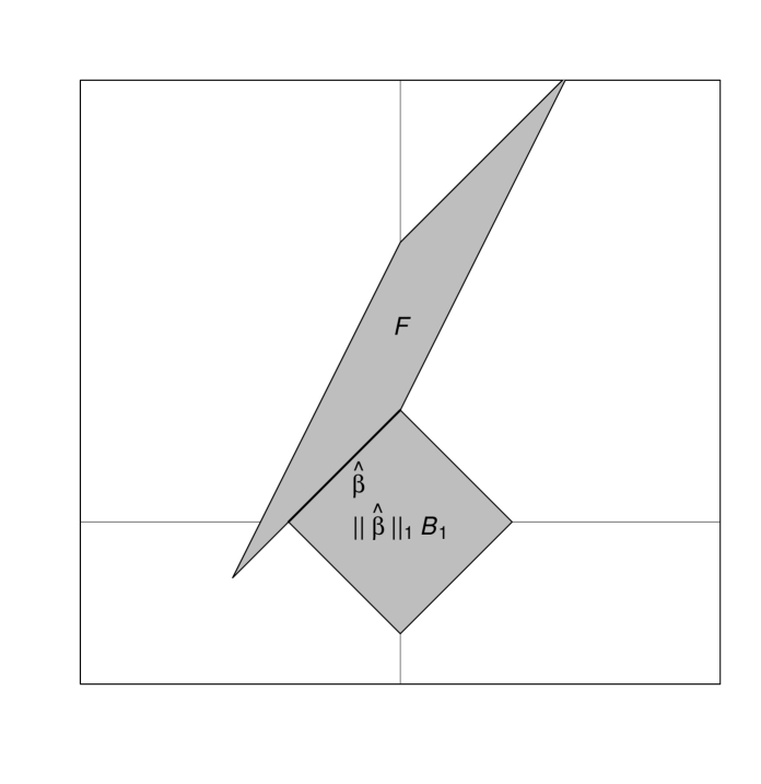
Figure 1: An instance of the Dantzig selector with multiple solutions. The region $F$ is the feasible set for the Dantzig selector and $||\hat{\beta}||_{1}B_{1}=\{u\in\mathbb{R}^{2};\ ||u||_{1}\leq||\hat{\beta}||_{1}\}$. The bold line represents the intersection of $||\hat{\beta}||_{1}B_{1}$ with $F$ and is the solution set for this instance of the Dantzig selector.

As indicated by the situation when $p=2$, if the Dantzig selector has multiple solutions, then $F$ is parallel to $B_{1}$ (Figure 1). When $p\geq 2$, the notion of parallelism which is correct for our purposes is less straightforward. Geometric intuition suggests that parallelism is invariant under translation and scalar multiplication, in the sense that $F$ is parallel to $B_{1}$ if and only if $\alpha F+\mathbf{v}_{0}=\{\alpha\boldsymbol{\beta}+\mathbf{v}_{0};\ \boldsymbol{\beta}\in F\}$ is parallel to $B_{1}$ for $a\in\mathbb{R}\setminus\{0\}$ and $\mathbf{v}_{0}\in\mathbb{R}^{p}$. In particular, multiplying $X$ by a (non-zero) scalar and adding vectors $\mathbf{y}_{0}\in\mathbb{R}^{n}$ to $\mathbf{y}$ does not affect parallelism. This leads to a definition of parallelism between $F$ and $B_{1}$ which depends only on the matrix $n^{-1}X^{T}X$. In fact, in our view, the primitive concept is parallelism between a $p\times p$ symmetric matrix $C$ and the $\ell^{1}$-ball.

Definition 1.

• Let $C$ be a $p\times p$ symmetric matrix. The matrix $C$ is parallel to the $\ell^{1}$-ball if and only if the condition [Par] (found below) holds.

• • There exist subsets $A,B\subseteq\{1,...,p\}$ and a vector $\mathbf{w}\in\mathbb{R}^{|B|}$ such that $||C_{B}\mathbf{w}||_{\infty}\leq 1$, $C_{A,B}\mathbf{w}\in\{\pm 1\}^{|A|}$, and $\dim\left[\mathrm{null}\left(C_{B,A}\right)\right]>0$.

• The feasible set for the Dantzig selector, $F$, is parallel to the $\ell^{1}$-ball if and only if $n^{-1}X^{T}X$ is parallel to the $\ell^{1}$-ball.

Remarks (i) Parallelism, as defined here, is related to degenerate sub-matrices of $C$, which, in the context of the Dantzig selector, correspond to the nontrivial faces of $F$. In [Par], the requirement that $C_{A,B}w\in\{\pm 1\}^{|A|}$ is related to the fact that the faces of the $\ell^{1}$-ball, $B_{1}$, have normal vectors $u\in\mathbb{R}^{p}$, where $u_{A}\in\{\pm 1\}^{|A|}$ for some $A\subseteq\{1,...,p\}$.

(ii) When $p=2$, it is easy to see that $F$ is parallel to the $\ell^{1}$-ball if and only if one of the columns of $n^{-1}X^{T}X$ is a scalar multiple of some point in $\{\pm 1\}^{2}$. This occurs if and only if a one-dimensional face of $F$ has slope 1 or -1, as depicted in Figure 1.

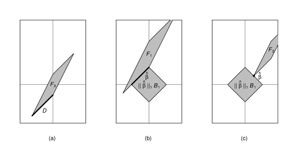
Figure 2: (a) $F_{0}=(X^{\prime}X)^{-1}B_{\infty}$ is parallel to the $\ell^{1}$-ball, as evidenced by the bold face $D$. (b) $F_{1}$ is obtained from $F_{0}$ by scalar multiplication and translation; the Dantzig selector problem with feasible set $F_{1}$ has multiple solutions, indicated by the bold line segment labeled $\hat{\beta}$. (c) $F_{2}$ is obtained from $F_{0}$ by scalar multiplication and translation; the point labeled $\hat{\beta}$ is the unique solution to the Dantzig selector problem with feasible set $F_{2}$.

As discussed above, parallelism is invariant under translation and scalar multiplication. On the other hand, translation and scalar multiplication of the feasible set $F$ gives rise to various instances of the Dantzig selector, some with a unique solution and some, perhaps, with multiple solutions. This suggests that any sufficient condition for the existence of multiple Dantzig selector solutions must, unlike parallelism, involve $\mathbf{y}$ and $\lambda$. To illustrate this concept, suppose that $n^{-1}X^{T}X$ is invertible and is parallel to the $\ell^{1}$-ball. Figure 2 (a) depicts $F_{0}=(n^{-1}X^{T}X)^{-1}B_{\infty}=\{(n^{-1}X^{T}X)^{-1}\mathbf{u};\ \mathbf{u}\in\mathbb{R}^{2},\ ||\mathbf{u}||_{\infty}\leq 1\}$, which is equal to the feasible set for the Dantzig selector when $\lambda=1$ and $\mathbf{y}=0$ and is parallel to the $\ell^{1}$-ball. Figures 2 (b) and (c) depict $F_{1}$ and $F_{2}$, potential feasible sets for the Dantzig selector that are both obtained from $F_{0}$ by scalar multiplication and translation. The feasible sets $F_{1}$ and $F_{2}$ are both parallel to the $\ell^{1}$-ball, and correspond to feasible sets for the Dantzig selector with the predictor matrix $X$ and different values for $\mathbf{y}$, $\lambda$ (not given here). The instance of the Dantzig selector with feasible set $F_{1}$ has multiple solutions, while the Dantzig selector with feasible set $F_{2}$ has a unique solution.

The following condition combines parallelism with additional constraints and is a sufficient condition for the existence of multiple Dantzig selector solutions.

[Mult]

There exist subsets $A,B\subseteq\{1,...,p\}$ and vectors $\boldsymbol{\mu}^{0}\in\mathbb{R}^{|B|}$, $\boldsymbol{\beta}^{0}\in F$, such that

• $||n^{-1}X^{T}X_{B}\boldsymbol{\mu}^{0}||_{\infty}\leq 1$, $n^{-1}X_{A}^{T}X_{B}\boldsymbol{\mu}^{0}\in\{\pm 1\}^{|A|}$, and $\dim\left[\mathrm{null}\left(n^{-1}X_{B}^{T}X_{A}\right)\right]>0$.

• $n^{-1}\boldsymbol{\beta}^{T}X^{T}X_{B}\boldsymbol{\mu}^{0}\geq||\boldsymbol{\beta}^{0}||_{1}$ for all $\boldsymbol{\beta}\in F$.

• $A=\{j;\ \beta_{j}^{0}\neq 0\}$.

• $n^{-1}|\mathbf{X}_{j}^{T}(\mathbf{y}-X\boldsymbol{\beta}^{0})|=\lambda$ for all $j\in B$ and $n^{-1}|\mathbf{X}_{j}^{T}(\mathbf{y}-X\boldsymbol{\beta}^{0})|<\lambda$ for all $j\notin B$.

Note that Condition 1 in [Mult] implies that $F$ is parallel to the $\ell^{1}$-ball. Conditions 2-4 in [Mult] constrain the location of $F$ in $\mathbb{R}^{p}$ relative to the origin. Proposition 1 below characterizes uniqueness properties of the Dantzig selector in terms of [Par] and [Mult]. A related necessary condition for the existence of multiple lasso solutions is given in Proposition 1 (c). Proposition 1 is proved in the Appendix at the end of this paper.

Proposition 1.

• If [Mult] holds, then the Dantzig selector has multiple solutions.

• If $F$ is not parallel to the $\ell^{1}$-ball, then the Dantzig selector has a unique solution.

• Suppose that $\lambda>0$ and that the lasso has multiple solutions (i.e. $\operatorname{argmin}\displaylimits_{\boldsymbol{\beta}\in\mathbb{R}^{p}}(2n)^{-1}||\mathbf{y}-X\boldsymbol{\beta}||^{2}+\lambda||\boldsymbol{\beta}||_{1}$ contains more than a single element). Then there exists a subset $A\subseteq\{1,...,p\}$ and a vector $w\in\mathbb{R}^{p}$ such that $||n^{-1}X^{T}X\mathbf{w}||_{\infty}\leq 1$, $n^{-1}X_{A}^{T}X\mathbf{w}\in\{\pm 1\}^{|A|}$, and $\dim\left[\mathrm{null}\left(n^{-1}X^{T}X_{A}\right)\right]>0$.

Remarks (i) Proposition 1 is valid for any $n$ and $p$.

(ii) Proposition 1 (c) may be rephrased as follows. If the lasso has multiple solutions, then $n^{-1}X^{T}X$ is parallel to the $\ell^{1}$-ball and, moreover, one may take $B=\{1,...,p\}$ in the definition of parallelism.

(iii) If $\lambda=0$, then the lasso has multiple solutions whenever $n^{-1}X^{T}X$ is singular.

(iv) The condition in Proposition 1 (c) implies that $n^{-1}X^{T}X$ is parallel to the $\ell^{1}$-ball. It follows that if $n^{-1}X^{T}X$ is not parallel to the $\ell^{1}$-ball, then both the Dantzig selector and lasso have unique solutions. The relationship between uniqueness for the Dantzig selector and uniqueness for lasso is discussed by Meinshausen et al. (2007), who give a concrete $p=3$-dimensional example (with pictures) where lasso has a unique solution, but the Dantzig selector does not.

(v) A condition similar to [Mult] which ensures the existence of multiple lasso solutions may be developed. This is not pursued further here .

The next proposition suggests that the Dantzig selector and lasso have a unique solution in an overwhelming majority of instances.

Proposition 2. Suppose that $\mathbf{x}_{1},...,\mathbf{x}_{n}$ are iid and drawn from a continuous distribution with respect to Lebesgue measure on $\mathbb{R}^{p}$. Then $n^{-1}X^{T}X$ is parallel to the $\ell^{1}$-ball with probability 0. Consequently, the Dantzig selector and lasso have a unique solution with probability 1.

Remarks (i) Proposition 2 is proved in the Appendix (a proof also appears in (Dicker, 2010)). To provide some intuition, note that the parallelism condition requires $n^{-1}X^{T}_{A}X_{B}$ to both (i) contain a specific point in its range (that is, an element of $\{\pm 1\}^{|A|}$) and (ii) to have a degenerate range (in the sense that $\dim\left[\mathrm{null}(n^{-1}X^{T}_{B}X_{A})\right]>0$). Proposition 2 implies that this occurs with probability 0, under the specified conditions.

4 Large sample asymptotics for the Dantzig selector

Throughout the rest of this article, assume that $p$ and $\boldsymbol{\beta}^{*}\in\mathbb{R}^{p}$ are fixed. In this section, we formulate the Dantzig selector as a well-defined mapping from sample covariance matrices, $n^{-1}X^{T}X$, marginal covariances, $n^{-1}X^{T}\mathbf{y}$, and tuning parameters, $\lambda\geq 0$, to estimators, $\hat{\boldsymbol{\beta}}^{ds}$. To do this, we restrict our attention to symmetric matrices that are not parallel to the $\ell^{1}$-ball – Proposition 2 suggests that this restriction is fairly weak. Then, we show that the Dantzig selector mapping is continuous. With this machinery in place, large sample asymptotics for the Dantzig selector follow easily.

Let $\mathscr{P}_{0}$ denote the collection of $p\times p$ positive semidefinite matrices that are not parallel to the $\ell^{1}$-ball and let $\mathscr{P}_{0}^{+}=\mathscr{P}_{0}\cap\mathrm{GL}(p)$, where $\mathrm{GL}(p)$ is the collection of all invertible $p\times p$ matrices with real entries. Define the Dantzig selector mapping $G:\mathscr{P}_{0}^{+}\times\mathbb{R}^{p}\times\mathbb{R}^{\geq 0}\to\mathbb{R}^{p}$ by $G(C,\mathbf{v},\lambda)=\hat{\mathbf{u}}$, where $\hat{\mathbf{u}}$ solves the optimization problem

$$\begin{array}[]{lc}\mbox{minimize}&||\mathbf{u}||_{1}\\ \mbox{subject to}&||C\mathbf{u}-\mathbf{v}||_{\infty}\leq\lambda.\end{array}$$ (4)

It follows directly from Proposition 1 (b) that $G$ is well-defined. Furthermore, notice that $G(n^{-1}X^{T}X,n^{-1}X^{T}\mathbf{y},\lambda)=\hat{\boldsymbol{\beta}}^{ds}$. Note that the domain of $G$ may be extended to a subset of $\mathscr{P}_{0}\times\mathbb{R}^{p}\times\mathbb{R}^{\geq 0}$, provided one imposes conditions to ensure that the feasible set in the optimization problem (4) is non-empty. More specifically, define $\mathscr{Q}=\{(C,\mathbf{v});\ C\in\mathscr{P}_{0},\ \mathbf{v}\in\mathrm{range}(C)\}$. Then (4) defines $G(C,\mathbf{v},\lambda)$ for $(C,\mathbf{v},\lambda)\in\mathscr{Q}\times\mathbb{R}^{\geq 0}$.

Proposition 3. The mapping $G$ is continuous on $\mathscr{P}_{0}^{+}\times\mathbb{R}^{p}\times\mathbb{R}^{\geq 0}$.

Remarks (i) A proof of Proposition 3 is found in the Appendix. A similar proof shows that $G$ is also continuous on $\mathscr{Q}\times\mathbb{R}^{>0}$. In other words, assuming that the appropriate (anti-) parallelism conditions hold, if there is non-trivial regularization in the limit (i.e. $\lambda_{n}\to\lambda_{0}>0$), then the Dantzig selector is continuous, regardless of whether or not the predictors and the limiting sample covariance matrix are singular.

Corollary 1. Suppose that $n^{-1}X^{T}X\to C\in\mathscr{P}_{0}^{+}$ and that $\lambda_{n}\to\lambda_{0}\geq 0$. Then $\hat{\boldsymbol{\beta}}^{ds}\to\boldsymbol{\beta}^{0}$, almost surely, where $\boldsymbol{\beta}^{0}$ solves

$$\begin{array}[]{lc}\mbox{minimize}&||\boldsymbol{\beta}||_{1}\\ \mbox{subject to}&||C(\boldsymbol{\beta}-\boldsymbol{\beta}^{*})||_{\infty}\leq\lambda_{0}.\end{array}$$

Remarks (i) The corollary follows directly from Proposition 3, which implies that $\hat{\boldsymbol{\beta}}^{ds}=G(n^{-1}X^{T}X,n^{-1}X^{T}\mathbf{y},\lambda_{n})\to G(C,C\boldsymbol{\beta}^{*},\lambda_{0})=\boldsymbol{\beta}^{0}$, almost surely.

(ii) Corollary 1 implies that under the given conditions, the Dantzig selector is consistent for $\boldsymbol{\beta}^{*}$ if and only if $\lambda_{n}\to 0$. Furthermore, it gives the almost sure limit of $\hat{\boldsymbol{\beta}}^{ds}$ in cases where the Dantzig selector is not consistent (that is, when $\lambda_{n}\to\lambda_{0}>0$).

Corollary 2. Suppose that $E(\epsilon_{i}^{2})=\sigma^{2}<\infty$. Also assume that $n^{-1}X^{T}X\to C\in\mathscr{P}_{0}^{+}$, that $\lim_{n\to\infty}n^{-1}\max_{1\leq i\leq n}||\mathbf{x}_{i}||^{2}=0$, and that $\sqrt{n}\lambda_{n}\to\tilde{\lambda}_{0}$. Let $A^{*}=\{j;\ \beta^{*}_{j}\neq 0\}$ and let $\bar{A}^{*}$ denote the complement of $A^{*}$ in $\{1,...,p\}$. Then $\sqrt{n}(\hat{\boldsymbol{\beta}}^{ds}-\boldsymbol{\beta}^{*})\stackrel{{\scriptstyle D}}{{\to}}\mathbf{u}^{0}$, where $\stackrel{{\scriptstyle D}}{{\to}}$ denotes convergence in distribution, $\mathbf{u}^{0}$ solves the optimization problem

$$\begin{array}[]{lc}\mbox{minimize}&||\mathbf{u}_{\bar{A}^{*}}||_{1}+\mathrm{sign}(\boldsymbol{\beta}^{*})_{A^{*}}^{T}\mathbf{u}_{A^{*}}\\ \mbox{subject to}&||C\mathbf{u}-\mathbf{v}^{0}||_{\infty}\leq\tilde{\lambda}_{0},\end{array}$$ (5)

and $\mathbf{v}^{0}\sim N(0,\sigma^{2}C)$.

Corollary 2 is proved in the Appendix.

Remarks (i) The second moment condition on $\epsilon_{i}$ and the condition $n^{-1}\max_{1\leq i\leq n}||\mathbf{x}_{i}||^{2}\to 0$ ensure that $n^{-1/2}X^{T}\boldsymbol{\epsilon}$ is asymptotically normal.

(ii) If $\tilde{\lambda}_{0}=0$, then $\hat{\boldsymbol{\beta}}^{ds}$ has the same asymptotic distribution as the ordinary least squares estimator. If $\tilde{\lambda}_{0}>0$, then the limiting distribution of the Dantzig selector is not normal.

(iii) Corollary 2 should be compared with Theorem 2 of (Knight and Fu, 2000), which describes the limiting distribution of $\hat{\boldsymbol{\beta}}^{lasso}$. Though the limiting distribution of lasso is determined by an unconstrained optimization problem, the term $||\mathbf{u}_{\bar{A}^{*}}||_{1}+\mathrm{sign}(\boldsymbol{\beta}^{*})_{A^{*}}^{T}\mathbf{u}_{A^{*}}$ in the limiting optimization problem for the Dantzig selector (5) also appears in the limiting optimization problem for lasso.

5 Discussion

The results in this paper address fairly long-standing open questions about uniqueness for the Dantzig selector and lasso. To summarize, we prove that the Dantzig selector and lasso estimators are unique in almost all instances. Though these results may appear to be somewhat esoteric, Proposition 2 and its corollaries demonstrate their potential usefulness. Indeed, we have shown that once uniqueness is understood, it is straightforward to obtain the almost sure limit and limiting distribution of Dantzig selector estimators. Taking a broader view, the results presented here may help clear the path for a more operator theoretic approach to studying the Dantzig selector, lasso, and other regularized regression procedures. Such an approach may offer additional insights into properties of these methods in a variety of settings. For instance, one could potential obtain a better understanding of the Dantzig selector in as asymptotic regime where $p\to\infty$, which is often of particular interest in regularized regression problems, by defining the Dantzig selector operator on an appropriate infinite dimensional space (analogous to the operator $G$ defined in Section 4 above) and studying its continuity properties in this more abstract setting. Future research in this direction is needed.

Appendix

Proof of Proposition 1. The following two lemmas establishes the Karush-Kuhn-Tucker (KKT) conditions for the Dantzig selector and lasso optimization problems. The lemmas appear in various forms in several references, including (Efron et al., 2007), (Asif, 2008), (Dicker, 2010), and (Asif and Romberg, 2010), and proofs are omitted.

Lemma A1. The vector $\hat{\boldsymbol{\beta}}=\hat{\boldsymbol{\beta}}^{ds}\in\mathbb{R}^{p}$ is a solution to the Dantzig selector (2) if and only if there is $\hat{\boldsymbol{\mu}}\in\mathbb{R}^{p}$ such that

$$n^{-1}||X^{T}(\mathbf{y}-X\hat{\boldsymbol{\beta}})||_{\infty} \leq \lambda$$ (6)

$$n^{-1}||X^{T}X\hat{\boldsymbol{\mu}}||_{\infty} \leq 1$$ (7)

$$n^{-1}\hat{\boldsymbol{\mu}}^{T}X^{T}X\hat{\boldsymbol{\beta}} = ||\hat{\boldsymbol{\beta}}||_{1}$$ (8)

$$n^{-1}\hat{\boldsymbol{\mu}}^{T}X^{T}(y-X\hat{\boldsymbol{\beta}}) = \lambda||\hat{\boldsymbol{\mu}}||_{1}.$$ (9)

Lemma A2. The vector $\hat{\boldsymbol{\beta}}=\hat{\boldsymbol{\beta}}^{lasso}\in\mathbb{R}^{p}$ is a solution to the lasso optimization problem (3) if and only if

$$\begin{array}[]{rcll}n^{-1}\mathbf{X}_{j}^{T}(\mathbf{y}-X\hat{\boldsymbol{\beta}})&=&\lambda\mathrm{sign}(\hat{\beta}_{j})&\mbox{if }\hat{\beta}_{j}\neq 0\\ |n^{-1}\mathbf{X}_{j}^{T}(\mathbf{y}-X\hat{\boldsymbol{\beta}})|&\leq&\lambda&\mbox{if }\hat{\beta}_{j}=0.\end{array}$$

To prove 1 (a), we assume that [Mult] holds and show that the Dantzig selector has multiple solutions. Let $\hat{\boldsymbol{\beta}}=\boldsymbol{\beta}^{0}$, $\hat{\boldsymbol{\mu}}=\boldsymbol{\mu}^{0}$, and $A,B\subseteq\{1,...,p\}$ be as in [Mult] and take $\mathbf{u}\in\mathbb{R}^{p}\setminus\{0\}$ so that $\mathbf{u}_{\bar{A}}=0$ and $n^{-1}X_{B}^{T}X_{A}\mathbf{u}_{A}=0$, where $\bar{A}$ is the complement of $A$ in $\{1,...,p\}$. Then it is clear from Lemma A1 that $\hat{\boldsymbol{\beta}}=\boldsymbol{\beta}^{0}$ is a solution to the Dantzig selector. Furthermore, using Lemma A1, it is easy to check that $\hat{\boldsymbol{\beta}}=\boldsymbol{\beta}^{0}+t\mathbf{u}$ is a solution to the Dantzig selector for $t\in\mathbb{R}$ sufficiently small (take $\hat{\boldsymbol{\mu}}=\boldsymbol{\mu}^{0}$).

Now suppose that $\boldsymbol{\beta}^{1},\boldsymbol{\beta}^{2}\in\mathbb{R}^{p}$ are distinct solutions to the Dantzig selector and let $\boldsymbol{\mu}^{1},\boldsymbol{\mu}^{2}\in\mathbb{R}^{p}$ be vectors such that $\hat{\boldsymbol{\beta}}=\boldsymbol{\beta}^{i}$ and $\hat{\boldsymbol{\mu}}=\boldsymbol{\mu}^{i}$, $i=1,2$ satisfy (6)–(9). Without loss of generality, assume that $\mathbf{s}=\mbox{sign}(\boldsymbol{\beta}^{1})=\mbox{sign}(\boldsymbol{\beta}^{2})$ and $\mathbf{r}=\mbox{sign}(\boldsymbol{\mu}^{1})=\mbox{sign}(\boldsymbol{\mu}^{2})$, where we define $\mbox{sign}(\boldsymbol{\beta})_{j}=\mbox{sign}(\beta_{j})=\beta_{j}/|\beta_{j}|$ or $0$, according to $\beta_{j}\neq 0$ or $\beta_{j}=0$, for $\boldsymbol{\beta}\in\mathbb{R}^{p}$. Let $A=\{j;\ \beta_{j}^{1}\neq 0\}=\{j;\ \beta_{j}^{2}\neq 0\}$, $B=\{j;\ \mu_{j}^{1}\neq 0\}=\{j;\ \mu_{j}^{2}\neq 0\}$. Then (7)–(8) imply that $||n^{-1}X^{T}X_{B}\boldsymbol{\mu}^{i}||_{\infty}\leq 1$ and $n^{-1}X_{A}^{T}X_{B}\boldsymbol{\mu}^{i}=\mathbf{s}\in\{\pm 1\}^{|A|}$, $i=1,2$. Additionally, (9) implies that $n^{-1}X_{B}^{T}X_{A}\boldsymbol{\beta}^{1}=n^{-1}X_{B}^{T}X_{A}\boldsymbol{\beta}^{2}$. Hence, $\dim\left[\mathrm{null}(n^{-1}X_{B}^{T}X_{A})\right]>0$. It follows that $n^{-1}X^{T}X$ is parallel to the $\ell^{1}$-ball.

Finally, to prove Proposition 1 (c), suppose

$$\boldsymbol{\beta}^{1},\boldsymbol{\beta}^{2}\in\operatorname{argmin}\displaylimits_{\boldsymbol{\beta}\in\mathbb{R}^{p}}\frac{1}{2n}||y-X\boldsymbol{\beta}||^{2}+\lambda||\boldsymbol{\beta}||_{1}$$

are distinct and suppose without loss of generality that $\mathbf{s}=\mbox{sign}(\boldsymbol{\beta}^{1})=\mbox{sign}(\boldsymbol{\beta}^{2})$. Let $A=\{j;\ \boldsymbol{\beta}^{1}_{j}\neq 0\}=\{j;\ \boldsymbol{\beta}^{2}_{j}\neq 0\}$ and $\mathbf{u}=\boldsymbol{\beta}^{2}-\boldsymbol{\beta}^{1}$. Notice that for $0\leq t\leq 1$ we have

$$\frac{1}{2n}\left\{2t\mathbf{u}^{T}X^{T}(\mathbf{y}-X\boldsymbol{\beta}^{1})-t^{2}\mathbf{u}^{T}X^{T}X\mathbf{u}\right\} = \frac{1}{2n}\left\{||\mathbf{y}-X\boldsymbol{\beta}^{1}||^{2}\right.$$ (10)

$$\qquad\left.-||\mathbf{y}-X(\boldsymbol{\beta}^{1}+t\mathbf{u})||^{2}\right\}$$

$$= \lambda t\mathbf{s}^{T}\mathbf{u}.$$

Since (10) must hold for all $0\leq t\leq 1$ and since $\lambda>0$, we must have $X\mathbf{u}=X_{A}\mathbf{u}_{A}=0$ and $\mathbf{s}^{T}\mathbf{u}=0$. It follows that

$$\mbox{dim}\left[\mbox{null}\left(n^{-1}X^{T}X_{A}\right)\right]>0$$ (11)

and $t=||\boldsymbol{\beta}^{1}||_{1}=||\boldsymbol{\beta}^{2}||_{1}$.

Now, let $\mathbf{w}=\lambda^{-1}[(X^{T}X)^{-}X^{T}\mathbf{y}-\boldsymbol{\beta}^{1}]\in\mathbb{R}^{p}$, where $(X^{T}X)^{-}$ is the Moore-Penrose pseudoinverse of $X^{T}X$. Then Lemma A2 implies that

$$n^{-1}||X^{T}X\mathbf{w}||_{\infty}=\frac{1}{n\lambda}||X^{T}(\mathbf{y}-X\boldsymbol{\beta}^{1})||_{\infty}\leq 1$$

and $n^{-1}X_{A}^{T}X\mathbf{w}=(n\lambda)^{-1}X_{A}^{T}(\mathbf{y}-X\boldsymbol{\beta}^{1})\in\{\pm 1\}^{|A|}$. Proposition 1 (c) follows from these observations plus (11). $\blacksquare$

Proof of Proposition 2. To prove Proposition 2, we make use of the following lemma.

Lemma A3. Suppose that $n\geq p$ and that the rows of $X$ are iid and drawn from a distribution which is continuous with respect to Lebesgue measure on $\mathbb{R}^{p}$. Let $W$ be an $n\times q$ matrix of rank $q\leq n$. Then $X^{T}W$ has rank $\min\{q,p\}$ with probability 1.

Proof of Lemma A3. Let $X$ and $W$ be as in the statement of the lemma. Without loss of generality, suppose that $q=p$. When $p=1$, the result is true. For $p>1$, let $[p]=\{1,...,p\}$. To facilitate a proof by induction, assume that $X_{[p-1]}^{T}W_{[p-1]}$ has rank $p-1$ with probability 1. On the event that $X_{[p-1]}^{T}W_{[p-1]}$ has rank $p-1$, the rank of $X^{T}W$ is less than $p$ if and only if

$$\mathbf{X}_{p}^{T}\left\{I-W_{[p-1]}(X_{[p-1]}^{T}W_{[p-1]})^{-1}X_{[p-1]}^{T}\right\}\mathbf{W}_{p}=0,$$ (12)

where $\mathbf{X}_{p}=X_{\{p\}}$ and $\mathbf{W}_{p}=W_{\{p\}}$. Since $W$ has full rank, it follows that

$$\left\{I-W_{[p-1]}(X_{[p-1]}^{T}W_{[p-1]})^{-1}X_{[p-1]}^{T}\right\}\mathbf{W}_{p}\neq 0,$$

with probability 1. Thus, conditioning on $X_{[p-1]}$ and using the fact that the conditional distribution of $\mathbf{X}_{p}$ is continuous, it follows that (12) holds with probability 0. We conclude that $X^{T}W$ has rank $p$ with probability 1. $\Box$

Getting back to the proof of Proposition 2, suppose that the rows of $X$ are iid and drawn from a distribution which is continuous with respect to Lebesgue measure on $\mathbb{R}^{p}$. Then $X$ has rank $\min\{n,p\}$ with probability 1. Let $A,B\subseteq\{1,...,p\}$ and decompose $A,B$ so that $A=A_{0}\cup J$, $B=B_{0}\cup J$, and $A_{0}$, $B_{0}$, and $J$ are disjoint. If $|A|>n$, then $X_{B}^{T}X_{A}$ has a non-trivial null space. Suppose for the moment that $|A|\leq n$. When $X$ has full rank, the dimension of the null space of $X_{B}^{T}X_{A}$ is non-zero if and only if

$$\dim\left(\mathrm{null}\left[X_{B_{0}}^{T}\left\{I-X_{J}(X_{J}^{T}X_{J})^{-1}X_{J}^{T}\right\}X_{A_{0}}\right]\right)>0.$$

Furthermore, if $X$ has full rank, then $\left\{I-X_{J}(X_{J}^{T}X_{J})^{-1}X_{J}^{T}\right\}X_{A_{0}}$ has full rank. Conditioning on $X_{A}$ and appealing to Lemma A3, it follows that the rank of $X_{B_{0}}^{T}\left\{I-X_{J}(X_{J}^{T}X_{J})^{-1}X_{J}^{T}\right\}X_{A_{0}}$ is $\min\{|A_{0}|,|B_{0}|\}$ with probability 1. Thus the null-space of $X_{B}^{T}X_{A}$ is non-trivial with positive probability if and only if $\min\{|B|,n\}<|A|$.

Now suppose that $\min\{|B|,n\}<|A|$. There are two cases: $|B|<|A|\leq n$ and $n<|A|$. In each case, the probability that there exists $\mathbf{w}\in\mathbb{R}^{|B|}$ such that $X_{A}^{T}X_{B}\mathbf{w}\in\{\pm 1\}^{|A|}$ is 0. We prove this for the case $|B|<|A|\leq n$; the case $n<|A|$ follows similarly. Assume that $|B|<|A|\leq n$. Choose $A_{1}\subseteq A_{0}$ such that $|A_{1}|=|B_{0}|$ and let $\tilde{A}=J\cup A_{1}$. Suppose that $X_{\tilde{A}}^{T}X_{B}\mathbf{w}=\mathbf{s}$ for some $\mathbf{s}\in\{\pm 1\}^{|\tilde{A}|}$ and $\mathbf{w}\in\mathbb{R}^{|B|}$. Then, assuming that $X$ is full rank,

$$\mathbf{w}_{J}=(X_{J}^{T}X_{J})^{-1}(\mathbf{s}_{J}-X_{J}^{T}X_{B_{0}}\mathbf{w}_{B_{0}})$$

and

$$X_{A_{1}}^{T}\left[\left\{I-X_{J}(X_{J}^{T}X_{J})^{-1}X_{J}^{T}\right\}X_{B_{0}}\mathbf{w}_{B_{0}}+X_{J}(X_{J}^{T}X_{J})^{-1}\mathbf{s}_{J}\right]=\mathbf{s}_{A_{1}}.$$

Thus, we have

$$\mathbf{w}_{B_{0}}=\left[X_{A_{1}}^{T}\left\{I-X_{J}(X_{J}^{T}X_{J})^{-1}X_{J}^{T}\right\}X_{B_{0}}\right]^{-1}\left\{\mathbf{s}_{A_{1}}-X_{A_{1}}^{T}X_{J}(X_{J}^{T}X_{J})^{-1}\mathbf{s}_{J}\right\},$$

where Lemma A3 guarantees that $X_{A_{1}}^{T}\left\{I-X_{J}(X_{J}^{T}X_{J})^{-1}X_{J}^{T}\right\}X_{B_{0}}$ is invertible with probability 1. Since, conditional on $X_{A_{1}\cup B}$, the rows of $X_{A_{0}\setminus A_{1}}$ are independent and have continuous distributions with respect to Lebesgue measure on $\mathbb{R}^{|A_{0}\setminus A_{1}|}$, it follows that

$$X_{A_{0}\setminus A_{1}}^{T}\!\left[\left\{I\!-\!X_{J}(X_{J}^{T}X_{J})^{-1}X_{J}^{T}\right\}X_{B_{0}}\mathbf{w}_{B_{0}}\!+\!X_{J}(X_{J}^{T}X_{J})^{-1}\mathbf{s}_{J}\right]\!\in\!\{\pm 1\}^{|A_{0}|-|A_{1}|}$$

with probability 0. Thus, as claimed, the probability that there exists $\mathbf{w}\in\mathbb{R}^{|B|}$ such that $X_{A}^{T}X_{B}\mathbf{w}\in\{\pm 1\}^{|A|}$ is 0.

The results from the last two paragraphs imply that

$$P\left[\begin{array}[]{c}\dim\left\{\mathrm{null}(X_{B}^{T}X_{A})\right\}>0\mbox{ and }\\ X_{A}^{T}X_{B}\mathbf{w}\in\{\pm 1\}^{|A|}\mbox{ for some}\ \mathbf{w}\in\mathbb{R}^{|B|}\end{array}\right]=0$$

It follows that $X^{T}X$ is parallel to the $\ell^{1}$-ball with probability 0, as was to be shown. $\blacksquare$

Proof of Proposition 3. For $n\in\mathbb{N}$, let $C_{n},C\in\mathscr{P}_{0}^{+}$, $\mathbf{v}_{n},\mathbf{v}\in\mathbb{R}^{p}$, and $\lambda_{n},\lambda\geq 0$ and assume that $C_{n}\to C$, $\mathbf{v}_{n}\to\mathbf{v}$, and $\lambda_{n}\to\lambda$. Let $\hat{\mathbf{u}}_{n}=G(C_{n},\mathbf{v}_{n},\lambda_{n})$ and let $\hat{\mathbf{u}}=G(C,\mathbf{v},\lambda)$. We show that $\hat{\mathbf{u}}_{n}\to\hat{\mathbf{u}}$.

Since $\sup_{n}||\hat{\mathbf{u}}_{n}||<\infty$, there exists a subsequence $\{\hat{\mathbf{u}}_{n_{k}}\}_{k=1}^{\infty}$ and a vector $\mathbf{u}_{0}\in\mathbb{R}^{p}$ such that $\hat{\mathbf{u}}_{n_{k}}\to\mathbf{u}_{0}$. To prove the proposition, it suffices to show that $\mathbf{u}_{0}=\hat{\mathbf{u}}$. By continuity of the $\ell^{\infty}$-norm, we must have

$$||C\mathbf{u}_{0}-\mathbf{v}||_{\infty}\leq\lambda.$$

Also, by the optimality properties of $\hat{\mathbf{u}}_{n_{k}}$, we must have

$$||\mathbf{u}_{0}||_{1}=\lim_{k\to\infty}||\hat{\mathbf{u}}_{n_{k}}||_{1}\leq\liminf_{k\to\infty}||\mathbf{w}_{n_{k}}||_{1}$$ (13)

for any sequence $\{\mathbf{w}_{n_{k}}\}$, with $\mathbf{w}_{n_{k}}\in\mathbb{R}^{p}$ and

$$||C_{n_{k}}\mathbf{w}_{n_{k}}-\mathbf{v}_{n_{k}}||_{\infty}\leq\lambda_{n_{k}}.$$ (14)

We consider two cases: $\lambda=0$ and $\lambda>0$. First suppose $\lambda=0$ and define $\mathbf{w}_{n_{k}}=C_{n_{k}}^{-1}(C\hat{\mathbf{u}}+\mathbf{v}_{n_{k}}-\mathbf{v})$. Then (14) holds and $\mathbf{w}_{n_{k}}\to\hat{\mathbf{u}}$. From (13), it follows that $||\mathbf{u}_{0}||_{1}\leq||\hat{\mathbf{u}}||_{1}$ and the optimality of $\hat{\mathbf{u}}$ implies that $\hat{\mathbf{u}}=\mathbf{u}_{0}$. Now suppose that $\lambda>0$ and define $\mathbf{w}_{n_{k}}=(\lambda_{n_{k}}/\lambda)C_{n_{k}}^{-1}(C\hat{\mathbf{u}}-\mathbf{v})+C_{n_{k}}^{-1}\mathbf{v}_{n_{k}}$. Then (14) holds and, as in the previous case, we conclude that $\hat{\mathbf{u}}=\mathbf{u}_{0}$. Thus, in either case, $\hat{\mathbf{u}}=\mathbf{u}_{0}$, as was to be shown. $\blacksquare$

Proof of Corollary 2. The conditions $E(\epsilon_{i}^{2})<\infty$ and $n^{-1}\max_{1\leq i\leq n}||\mathbf{x}_{i}||^{2}\to 0$ ensure that $n^{-1/2}X^{T}\boldsymbol{\epsilon}\stackrel{{\scriptstyle D}}{{\to}}\mathbf{v}^{0}\sim N(0,\sigma^{2}C)$, by the Lindeberg-Feller central limit theorem. By the Skorokhod representation theorem, we may assume without loss of generality that $n^{-1/2}X^{T}\boldsymbol{\epsilon}\to\mathbf{v}^{0}$ almost surely.

Now let $\mathbf{u}=\sqrt{n}(\boldsymbol{\beta}-\boldsymbol{\beta}^{*})$ and notice that the Dantzig selector (2) is equivalent to the optimization problem

$$\begin{array}[]{lc}\mbox{minimize}&||\sqrt{n}\boldsymbol{\beta}^{*}+\mathbf{u}||_{1}\\ \mbox{subject to}&\left|\left|n^{-1}X^{T}X\mathbf{u}-n^{-1/2}X^{T}\boldsymbol{\epsilon}\right|\right|_{\infty}\leq\sqrt{n}\lambda_{n}.\end{array}$$ (15)

In particular, $\hat{\mathbf{u}}=\sqrt{n}(\hat{\boldsymbol{\beta}}^{ds}-\boldsymbol{\beta}^{*})$ solves (15). We show that $\hat{\mathbf{u}}\to\mathbf{u}^{0}$, the solution to (5), almost surely. This suffices to prove the corollary.

Since $n^{-1}X^{T}X\to C$, $n^{-1/2}X^{T}\boldsymbol{\epsilon}\to\mathbf{v}^{0}$ almost surely, and $\sqrt{n}\lambda_{n}\to\tilde{\lambda}_{0}$, it follows that there is an almost surely finite random variable $M$ such that $||\mathbf{u}||_{\infty}\leq M/2$ whenever $\mathbf{u}$ is feasible for the optimization problem (15). Let $\mathbf{s}=\mathrm{sign}(\boldsymbol{\beta}^{*})$ and notice that if $\sqrt{n}\min\{|\beta_{j}^{*}|;\ j\in A^{*}\}>M$ and $\mathbf{u}$ is feasible for (15), then $\mathrm{sign}(\sqrt{n}\boldsymbol{\beta}^{*}+\mathbf{u})=\mathrm{sign}(M\mathbf{s}+\mathbf{u})$. It follows that

$$G(n^{-1}X^{T}X,n^{-1/2}X^{T}\boldsymbol{\epsilon}+n^{-1}X^{T}XM\mathbf{s},\sqrt{n}\lambda_{n})=M\mathbf{s}+\hat{\mathbf{u}}$$

whenever $\sqrt{n}\min\{|\beta_{j}^{*}|;\ j\in A^{*}\}>M$. Taking $n\to\infty$, Proposition 3 implies that $\hat{\mathbf{u}}\to G(C,\mathbf{v}^{0}+CM\mathbf{s},\tilde{\lambda}_{0})-M\mathbf{s}$ almost surely and it is straightforward to check that $\mathbf{u}^{0}=G(C,\mathbf{v}^{0}+CM\mathbf{s},\tilde{\lambda}_{0})-M\mathbf{s}$. $\blacksquare$

References

• Asif (2008) Asif, M. (2008). Primal Dual Pursuit: A Homotopy Based Algorithm for the Dantzig Selector. Master’s thesis, Georgia Institute of Technology, USA.
• Asif and Romberg (2010) Asif, M. and J. Romberg (2010). On the lasso and Dantzig selector equivalence. In 44th Annual Conference on Information Sciences and Systems (CISS), pp.  1–6. IEEE.
• Bickel and Li (2006) Bickel, P. and B. Li (2006). Regularization in statistics. Test 15(2), 271–344.
• Bickel et al. (2009) Bickel, P., Y. Ritov, and A. Tsybakov (2009). Simultaneous analysis of lasso and Dantzig selector. Annals of Statistics 37(4), 1705–1732.
• Candès and Tao (2007) Candès, E. and T. Tao (2007). The Dantzig selector: Statistical estimation when $p$ is much larger than $n$. Annals of Statistics 35(6), 2313–2351.
• Dicker (2010) Dicker, L. (2010). Regularized Regression Methods for Variable Selection and Estimation. Ph.D. thesis, Harvard University, USA.
• Efron et al. (2007) Efron, B., T. Hastie, and R. Tibshirani (2007). Discussion: The Dantzig selector: Statistical estimation when $p$ is much larger than $n$. Annals of Statistics 35(6), 2358–2364.
• Fan and Lv (2010) Fan, J. and J. Lv (2010). A selective overview of variable selection in high dimensional feature space. Statistica Sinica 20(1), 101–148.
• James et al. (2009) James, G., P. Radchenko, and J. Lv (2009). DASSO: Connections between the Dantzig selector and lasso. Journal of the Royal Statistical Society: Series B 71(1), 127–142.
• Knight and Fu (2000) Knight, K. and W. Fu (2000). Asymptotics for lasso-type estimators. Annals of Statistics 28(5), 1356–1378.
• Meinshausen et al. (2007) Meinshausen, N., G. Rocha, and B. Yu (2007). Discussion: A tale of three cousins: Lasso, L2Boosting and Dantzig. Annals of Statistics 35(6), 2373–2384.
• Tibshirani (1996) Tibshirani, R. (1996). Regression shrinkage and selection via the lasso. Journal of the Royal Statistical Society: Series B 58(1), 267–288.
• Tibshirani (2011) Tibshirani, R. (2011). Regression shrinkage and selection via the lasso: a retrospective. Journal of the Royal Statistical Society: Series B 73(3), 273–282.