Planetary and Other Short Binary Microlensing Events
from the MOA Short Event Analysis

Abstract

We present the analysis of four candidate short duration binary microlensing events from the 2006-2007 MOA Project short event analysis. These events were discovered as a byproduct of an analysis designed to find short timescale single lens events that may be due to free-floating planets. Three of these events are determined to be microlensing events, while the fourth is most likely caused by stellar variability. For each of the three microlensing events, the signal is almost entirely due to a brief caustic feature with little or no lensing attributable mainly to the lens primary. One of these events, MOA-bin-1, is due to a planet, and it is the first example of a planetary event in which stellar host is only detected through binary microlensing effects. The mass ratio and separation are $q=4.9\pm 1.4\times 10^{-3}$ and $s=2.10\pm 0.05$, respectively. A Bayesian analysis based on a standard Galactic model indicates that the planet, MOA-bin-1Lb, has a mass of $m_{p}=3.7\pm 2.1M_{\rm Jup}$, and orbits a star of $M_{\ast}=0.75{+0.33\atop-0.41}M_{\odot}$ at a semi-major axis of $a=8.3{+4.5\atop-2.7}\,$AU. This is one of the most massive and widest separation planets found by microlensing. The scarcity of such wide separation planets also has implications for interpretation of the isolated planetary mass objects found by this analysis. If we assume that we have been able to detect wide separation planets with a efficiency at least as high as that for isolated planets, then we can set limits on the distribution on planets in wide orbits. In particular, if the entire isolated planet sample found by Sumi et al. (2011) consists of planets bound in wide orbits around stars, we find that it is likely that the median orbital semi-major axis is $>30\,$AU.

1 Introduction

Gravitational microlensing plays a unique role among methods to search for exoplanets because planets can be detected without the detection of any light from the host star (Bennett, 2008; Gaudi, 2010). In fact, old, planetary mass objects can be detected even in cases when there is no indication of a host star (Sumi et al., 2011). This contrasts with the Doppler radial velocity (Butler et al., 2006; Bonfils et al., 2011) and transit (Borucki et al., 2011) methods, which rely on the precision measurements of light from the source star to the signals needed to detect the planets.

Until 2011, the primary implication of the microlensing searches for exoplanets was the relatively large number of cold planets orbiting sub-solar-mass stars (Sumi et al., 2010; Gould et al., 2010b; Cassan et al., 2012). Microlensing is primarily sensitive to planets beyond the snow line, where the proto-planetary disk is cold enough for ice to condense. The snow line (Ida & Lin, 2005; Lecar, 2006; Kennedy et al., 2006; Kennedy & Kenyon, 2008; Thommes et al., 2008) is of great importance in the core accretion theory. Ices can condense beyond the snow line, and this increases the density of solid material in the proto-planetary disk by a factor of a few, compared to the disk just inside the snow line. This high density of solids beyond the snow line is needed to form the ice-rock cores that can grow massive enough to accrete significant amounts of hydrogen and helium gas to become gas giants. But, it is also thought that this process may often be terminated before the final gas accretion phase, particularly for low-mass stellar hosts (Laughlin et al., 2004), This leaves a large number of $\sim 10{M_{\oplus}}$ “failed jupiter” planets, which are consistent with the microlensing observations.

A somewhat more unexpected discovery was reported by Sumi et al. (2011) who have analyzed the first two years of the MOA-II Galactic bulge microlensing survey data, and found an excess of events with an Einstein radius crossing time of $t_{E}<2\,$days. This excess could not be explained by an extrapolation of the brown dwarf mass function into the planetary mass regime, and so a previously undetected population of isolated planetary mass objects was needed to explain it. Such a population is expected to arise from a variety of processes, such as planet-planet scattering (Levison et al., 1998; Ford & Rasio, 2008; Guillochon et al., 2011), star-planet scattering (Holman & Wiegert, 1999; Musielak et al., 2005; Doolin & Blundell, 2011; Malmberg et al., 2011; Veras & Raymond, 2012), and stellar death (Veras et al., 2011). However, Sumi et al. (2011) find that this new population consists of $1.8{+1.7\atop-0.8}$ times as many $\sim 1$ Jupiter-mass objects as main sequence stars, and this is somewhat larger than expected. But, as Sumi et al. (2011) show, the number of bound planets found by microlensing is similar to the number of planets in the new isolated planet population.

The planetary mass objects in this newly discovered population are isolated in the sense that there is no host star that can be detected in the microlensing data. This implies a lower limit on the projected separation between the planet and a possible host star that depends on the hypothetical host star’s Einstein radius. The lower limits reported by Sumi et al. (2011) range from 2.4 to $15.0\,R_{E}$, which corresponds to 7-$45\,$AU, assuming typical host star masses and random orientations. The fact that distant host star are not strongly excluded has led some (Nagasawa & Ida, 2011; Wambsganss, 2011) to suggest that many of these isolated planets may, in fact, be bound in distant orbits to host stars. Others have even suggested that the large number of isolated planets may be due to an in situ formation mechanism (Bowler et al., 2011) that differs from the core accretion theory (Lissauer, 1993).

It remains uncertain, however, if most of the planets in this newly discovered isolated planet population are truly unbound, or orbiting stars in very wide orbits. And if a significant fraction of these isolated planets do orbit stars, it is unclear if they might have formed somewhat closer to their host stars (near the snow line) and moved outwards since their formation. Alternatively, distant bound planets could have formed in situ by gravitational instability (Boss, 1997).

These questions can be addressed with microlensing survey data by identifying microlensing events due to planets in very wide orbits. When we are lucky enough to have the relative motion of the lens and source stars align with the planet-star separation vector, then it is possible to detect the star-planet system as two single lens light curves that are widely separated in time (Di Stefano & Scalzo, 1999). But, if the planet-star separation is not too large, it is also possible to detect the binary lens effects of the distant host star through a close approach of the source star with the planetary caustic (Han & Kang, 2003; Han et al., 2005). These appear as short duration binary microlensing events, but not all short duration binary lensing events are due to low-mass lens systems. Stellar binary lenses will generate small caustics if their separation is much smaller than the Einstein radius. It is also possible to have a short caustic crossing feature in a much longer duration microlensing event, and if the source is faint, it may be difficult to detect the microlensing magnification outside of the caustic if the source is blended with brighter stars. So, detailed modeling of the observed binary events is needed to determine which of these scenarios provides the correct description of a given microlensing event.

The main background for short duration microlensing events is variable stars with a short duration, such as cataclysmic variables (CVs) or flare stars, as discussed by Sumi et al. (2011). Such variables are much more common than short duration microlensing events, but they can generally be distinguished from microlensing events because their light curves are poorly fit with microlensing models. However, it is more difficult to distinguish between variable stars and binary microlensing events because the binary events are described by 3 or 4 additional parameters. If there are a small number of data points sampling the important light curve features, it will be much easier to fit a variable star light curve with a binary lens model than with a single lens model.

In this paper, we present the analysis of four light curves from the analysis of Sumi et al. (2011). These light curves all exhibit short timescale brightenings that can be well fit by binary microlensing light curves. Following Bond et al. (2004), we define events with a mass ratio of $q\leq 0.03$ as planetary events, while a mass ratio of $q>0.03$ would imply a brown dwarf secondary. We find that one of these events, MOA-bin-1, is due to microlensing by a wide-separation planet, which is separated from its host star by more than two Einstein radii. Two of the events, MOA-bin-2 and MOA-bin-3, are best fit with binary models with brown dwarf mass ratio secondaries. The final event has a light curve that is best fit by a primary lens of about a Jupiter mass, orbited by a secondary of a few Earth-masses. However, the brightening is extremely short, and the apparent binary lens features are just barely sampled by the observations. Thus, they may be fit by a binary lens model because such a model has enough adjustable parameters to fit the observations. Unlike the case of MOA-bin-1, the apparent microlensing light curve features are not oversampled, so the observations do not definitively demonstrate that the features are due to microlensing. It seems most likely that, despite the good microlensing fit, the brightening is due to a large amplitude stellar flare.

This paper is organized as follows. In Section 2, we describe the data analysis and the selection of events to analyze in this paper. Section 3 presents the details of the light curve analysis for each of the four events that we consider, and we present our analysis of the physical properties of the MOA-bin-1L planetary system in Section 4. We discuss the implications of these and similar events in resolving the puzzles raised by our recent discovery (Sumi et al., 2011) of a large population of isolated planetary mass lens masses in Section 5, and we summarize our conclusions in Section 6. In Appendix A, we further discuss the rationale for excluding non-planetary models for MOA-bin-1, and finally, in the Appendix B, we present an analysis of the source star colors for two of the three binary lensing events presented in this paper, plus the 10 isolated planet events from (Sumi et al., 2011). For five of these events the Optical Gravitational Lensing Experiment (OGLE) data allows us to use an improved version of the MOA-OGLE color method introduced by Gould et al. (2010a). This analysis shows that the source stars are likely to be normal bulge main sequence or sub-giant stars, although in two of these five cases, the color of the source star is difficult to determine due to microlensing model uncertainties.

2 Data Analysis and Event Selection

The light curve analysis presented here is based on the data analysis and preliminary event selection of Sumi et al. (2011), which is discussed in some detail in the Supplementary Information for that paper. This analysis uses the 2006-2007 MOA-II galactic bulge survey data, which consist of $\sim 8250$ images of each of the two most densely sampled fields (fields gb5 and gb9) and 1660-2980 images of each of the 20 other less densely sampled fields. The bulge was observed for about 8 months of each year from the end of February to the beginning of November. This observing strategy is designed to detect short duration single lens events and short timescale anomalies in the light curves of stellar microlensing events due to planets orbiting the lens stars (Mao & Paczyński, 1991; Bennett, 2008; Gaudi, 2010). The MOA images were reduced with MOA’s implementation (Bond et al., 2001) of the difference image analysis (DIA) method (Tomaney & Crotts, 1996; Alard & Lupton, 1998).

The images were taken using the custom MOA-Red wide-band filter, which is approximately equivalent to the sum of the standard Kron/Cousins $R$ and $I$-bands, and the photometry was approximately calibrated to the Kron/Cousins $I$-band using OGLE-II photometry map of the Galactic bulge (Udalski et al., 2002), as described by Sumi et al. (2011). In this paper we improve upon this calibration with a more careful comparison to the OGLE-III photometry catalog (Szymański et al., 2011).

Candidate short duration binary microlensing events were selected following the procedure of Sumi et al. (2011), using cuts 0 and 1 to identify select events. The 5-parameter microlensing fits used for Sumi et al. (2011) cut-2 were used to help identify short duration events, but these 5-parameter fits can sometimes fail to identify short duration events due to a well known degeneracy (Alard, 1997; Di Stefano & Esin, 1995) between short events with bright sources and long events with faint sources. Therefore, we also measured event durations with a simple top-hat filter that uses the duration of consecutive measurements that are $>3\sigma$ above the baseline. All the events with at least 10 observations $>3\sigma$ above the baseline and best fit single lens $t_{E}$ values or top-hat filter durations of $<3\,$days were examined by eye in addition to all events with best fit single lens events with $t_{E}<3\,$days. The sample examined by eye consisted of 149 events, and this sample overlapped with 8421 events of all durations classified by eye during the Sumi et al. (2011) analysis. About 40 of these events were fit with microlensing models. Most of the events that were well fit by microlensing models were well fit by single lens models. These included the 10 single lens events of Sumi et al. (2011), and a similar number of other events that were well fit by single lens models, but did not pass all of the Sumi et al. (2011) selection criteria (usually due to poor light curve coverage or blending uncertainties). The 18 events from this sub-sample that were not well fit by single lens models, were then fit by binary lens models. Most of these events could not be fit with a binary lens model, and they are likely to be cataclysmic variables (CVs) with sharp changes the light curve slope that are superficially similar to caustic entry features. A few other events were too poorly sampled to yield a unique solution. This left the 4 events with good, short duration binary microlensing models that we present in this paper. The coordinates of these events are listed in Table 1.

Although this procedure is somewhat subjective, it is unlikely that any real, short duration, binary microlensing events were missed, as long as they passed cuts 0 and 1 of Sumi et al. (2011). The primary backgrounds for the identification of short binary microlensing events are short single-lens events and CVs. But, single lens events can all be identified by their single lens fits (which were already done by Sumi et al. (2011). CV light curves typically look very different from microlensing event light curves, and we have fit all the light curves that have a remote possibility of being due to microlensing. So, it is unlikely that any binary microlensing events have been missed by this procedure. The one thing missing from this analysis is that we have not determined the detection efficiency for these short binary lens events.

As in the case of the Sumi et al. (2011) analysis, once the events were identified, we requested contemporaneous OGLE-III data from the OGLE collaboration. Unfortunately, for 3 of the 4 light curves we present, there is no OGLE-III data for the star in question during the year that the event occurred. And for MOA-bin-1, the event with OGLE-III, coverage, the OGLE observations are limited to times of modest magnification. The lack of signal in the OGLE data makes it difficult to identify the location of the lensed source in the OGLE images, particularly when the images with the most significant magnification have poor seeing, as is the case for MOA-bin-1. In this case, OGLE have reported the photometry at the location of an apparent star identified in their reference frames, which is 2-3 times brighter than the source star, so it is possible that the source location is significantly offset from the location used for the photometry. This could lead to systematic errors in the OGLE photometry for this event.

2.1 Correction for Systematic Photometry Errors

Two of these events had evidence for systematic photometry errors in the original photometry of the event. As is generally the case in microlensing analyses, these systematic errors are not large enough to have an effect on the event selection. Instead they affect the interpretation of individual events.

The photometry of MOA-bin-3 originally showed systematic nightly variations that were correlated with seeing, and different reductions favored a close-binary, brown-dwarf secondary model or a wide binary, planetary secondary model. Both models can produce light curve shapes that are very similar during the times that are sampled by the MOA data. So, it was worthwhile to see if photometric re-reductions could improve the photometry of this event. The MOA images for this event were re-reduced several times with different choices for the reference images. These re-reductions used the so-called “cameo” images, which are sub-frames of the original images, centered on the location of the event. We selected a cameo data set which had a negligible correlation between the seeing and the photometry in the unmagnified part of the light curve.

The original MOA photometry for MOA-bin-1 also showed evidence of systematic photometry errors. A telltale sign of the problem for this event was a systematic pattern of residuals in the difference images taken at high airmass. The direction of this systematic residuals varied with the observing season, which implies that they are likely to be caused by differential refraction. Such photometry problem could be caused by the effect of differential refraction on bright reference stars that are used to register the images if these stars have different colors. Similar photometry errors might also arise if the target star is blended with a star with a different color. The effect of these photometry errors could also be seen in the binned MOA light curves as a slow decrease in brightness for each season, which continued in the later seasons that weren’t included in this analysis.

To correct for this systematic error, we fit the photometry outside of the microlensing event with a general quadratic function depending on $(\cos\psi/\cos z)$ and $(\sin\psi/\cos z)$, where $z$ is the angle between the target position and zenith and $\psi$ is the direction of differential refraction. ($1/\cos z=\,$airmass.) This quadratic model is then used to correct the photometry, resulting in an improvement $\Delta\chi^{2}=789.7$ for the 7232 MOA observations, implying an average improvement of $\sigma/3$. The systematic photometry trend over each season is largely removed by this correction. Such a low-level systematic error does not have any significant effect on the shape of the cusp crossing feature that led to selection of this event, but it does effect the lower level variation of the light curve before and after the cusp crossing, which are primarily due to the stellar host star. Thus, correction of this systematic error was crucial for determining the properties of the host star for this planet.

3 Light Curve Analysis

The light curve modeling for this paper was done with the modeling code of Bennett (2010) with a few modifications. First, the light curve calculations now make use of the hexadecapole approximation (Gould, 2008; Pejcha & Heyrovsky, 2009) in situations when finite source effects are important but not extremely strong. Full numerical integration is used whenever there is a caustic crossing, and when there is no caustic crossing, the hexadecapole approximation is used when the difference between both the hexadecapole and quadrapole and the quadrapole and point source approximations are relatively small. When the difference between one pair of these lower order approximations becomes too large, the full numerical integration as described in Bennett (2010) is used.

An additional modification is needed to deal with events that are dominated by caustic features which are far from the center of mass. Such events can approach the Chang-Refsdahl approximation (Chang & Refsdal, 1979, 1984), where the gravitational field encountered by the light rays from the source is dominated by a single mass plus the gradient of a gravitational field from a more distant mass. This gradient field is parameterized by the shear $\gamma$, which is given by $\gamma=1/d_{\rm dist}^{2}$, where $d_{\rm dist}$ is the separation of the distant mass measured in units of its Einstein radius. This shear approximation has been used for theoretical studies of extrasolar planets detected by microlensing (Gould & Loeb, 1992), and this is useful for a theoretical understanding of what parameters can be constrained in events like this. If we instead express the shear in units of the nearby mass it becomes $\gamma=q/d_{\rm near}^{2}$, where $q$ is the mass ratio of the distant to the nearby mass, and $d_{\rm near}$ is the separation in units of the Einstein radius of the nearby mass. This holds because the Einstein radii for the distant and nearby masses scales as $\sim\sqrt{q}$. Thus, models with similar values of $\gamma$, but very different values of $d_{\rm near}$ and $q$ will give very similar light curve shapes. So, the shear approximation is a good guide to indicate possible light curve degeneracies, but this approximation is not accurate enough to use for light curve modeling and does not reduce the need for time consuming numerical calculations.

The main difficulty with using general purpose light curve modeling codes for modeling the events we present in this paper is that it is awkward to us use polar coordinates centered far from the location of lens features giving rise to the observed magnification. The region of parameter space that must be sampled is the region of significant magnification, and this is not located at the center-of-mass for the system or at the locations of either of the lens masses. Instead, the locations of significant magnification are located at the positions of the caustics. So, for most of the modeling used in this paper, we define the coordinate center to be the centroid of the caustic curve, which is approached or crossed by the source. This centroid is defined numerically from a set of caustic points that have been transformed, using the lens equation from a set of points that are equally spaced on the critical curve in the image plane. Once in the general vicinity of the solution, however, the use of the parameter correlation matrix with the Metropolis algorithm, as described by Bennett (2010) is sufficient to deal with the parameter correlations in the center-of-mass coordinate system.

This caustic centered modeling approach is not entirely general. First, since the caustic locations are only known numerically, the centroid of a caustic will have some dependence on numerical parameters. But, a more serious issue occurs when the lens parameters change in such a way that the caustics would merge. This would cause a sudden, discontinuous change in the location of the center of the coordinate system, that would likely cause the fitting code to fail. So, this code is only used in situations when reconnection of the caustics is unlikely, and modeling for this paper has generally been performed in parallel using the caustic centered approach in parallel with the standard center-of-mass centered approach.

For each of the four events presented in this paper, we have done a systematic search for binary lens models following the method of Bennett (2010), but using the caustic-centered coordinate system. For events MOA-bin-1 and MOA-bin-2, which are dominated by a single cusp crossing and caustic crossing feature, respectively, we also did a search based on these observed features. For MOA-bin-1, we investigated models in which the source crossed each of the caustics of a binary lens system, including wide and close binaries, as well as the so-called resonant systems, which have only a single connected caustic curve. For MOA-bin-2, we explicitly considered all geometries of caustic crossing binaries. In both cases, the results were identical to the results from the initial condition grid search method of Bennett (2010), using the caustic-centered coordinate system.

3.1 MOA-bin-1

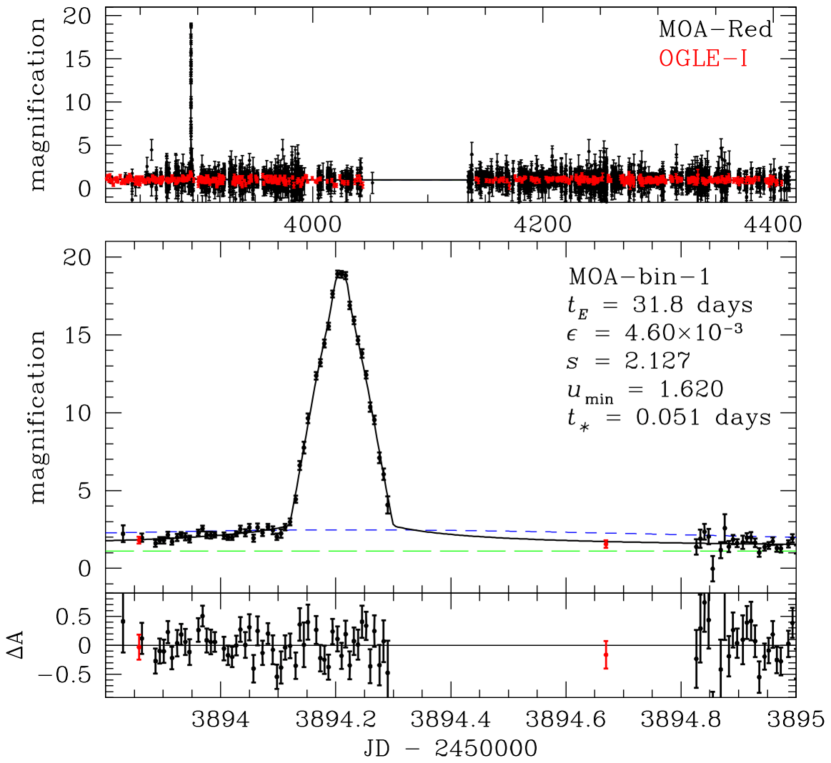
Figure 1: The light curve of event MOA-bin-1 in field gb5 with a $\sim 10\,$min sampling cadence. The top panel shows the 2006-2007 MOA-red and OGLE I-band data; the middle panel shows a close up of the light curve peak, and the bottom panel shows the residuals from the best fit. The blue, short-dashed curve and green, long-dashed curves show the single lens light curves due to planet and host star, respectively. As described in the text, the OGLE data are not used in the fit, but are added to the plot based on the cross-calibration of the OGLE and MOA photometry.

The light curve of the planetary event MOA-bin-1 is shown in Fig. 1. This event is in the gb5 field, which had a $\sim 10\,$minute sampling cadence, and it has an inverted-V cusp crossing feature that is almost completely resolved by the MOA observations. Such a feature is readily recognized as a characteristic microlensing feature due to a caustic crossing very close to a cusp, such that the separation of the caustic crossings along the source trajectory is similar to or smaller than the source star diameter. (The brief, $\sim 20\,$minute duration flat peak of the light curve indicates that the width of the caustic is just slightly larger than the source.)

Unfortunately, the bright MOA-bin-1 cusp crossing feature occurred during daylight hours at the OGLE telescope, and the OGLE data contain only three relatively poor seeing observations with a magnification as large as $A>1.5$. These were not sufficient to identify the centroid of the of the event, so the photometry is done at the location of a “star” in the OGLE reference frame. This means that there are likely to be blending-related systematic errors in the OGLE photometry. Therefore, we do not include the OGLE data in our fits, but we plot the OGLE data in Fig. 1 according to the color transformation discussed in Section 4, assuming a source star color consistent with an Hubble Space Telescope (HST) color magnitude diagram (CMD), as discussed in Bennett et al. (2008). This puts the photometry from the relatively poor seeing OGLE data near the peak of the event on the curve, as indicated in Fig. 1, but the photometry from better seeing images at lower magnification does not fit so well due to the offset between the location of the “star” seen in the OGLE images and the location of the source star.

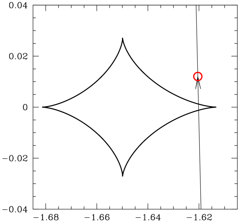
Figure 2: The caustic geometry for the best fit MOA-bin-1 model. The red circle indicates the best fit source size, and the coordinates for this plot are centered at the center-of-mass of the full lens system (both the planet and its host star). The coordinates are given in units of the Einstein radius of the lens system. The source trajectory is nearly perpendicular to the lens axis. There is a degenerate fit, with $\chi^{2}$ larger by $\Delta\chi^{2}=0.199$, that has a nearly identical caustic configuration, except that the source crosses the outer cusp instead of the inner one.

The best fit model for MOA-bin-1, was found using the initial parameter grid search method outlined in Bennett (2010), but a caustic centered coordinate system was used, as described above. This procedure yielded two nearly degenerate solutions, with a $\chi^{2}$ difference of $\Delta\chi^{2}=0.428$. These solutions have a nearly identical geometry, with the main difference being that the slightly favored solution crosses the inner cusp of the planetary caustic, while the second best solution crosses the outer cusp. The favored solution is the one indicated in Fig. 2. There are also disfavored solutions in which the source crosses the top or bottom cusps in Fig. 2. These differ from the inner and outer cusp crossing solutions because the source must also approach the primary lens caustic. If there are systematic errors in the baseline part of the light curve, the $\chi^{2}$ might be improved if the peak due to an approach to the primary caustic occurs at the same time as a light curve bump due to systematic photometry errors. When we are close to the Chang-Refsdal limit, the main light curve features do not really constrain where such a peak might occur, so the fitting code will naturally adjust the parameters to put this feature in the location that will minimize the $\chi^{2}$. It is therefore important to correct systematic photometry errors in the baseline photometry, as discussed in Section 2.1.

In this case, we find that the solutions which cross the top or bottom cusp of the planetary caustic, are disfavored by $\Delta\chi^{2}=17.5$. Formally, this is enough to strongly exclude them. However, at $4135<t<4200$, the top or bottom cusp crossing models are favored over the inner and outer cusp crossing models by $\Delta\chi^{2}=16.6$. Most likely, this is simply due a small systematic error and/or random noise, so the top or bottom cusp crossing solutions should be disfavored by $\Delta\chi^{2}\sim 34.1$. The parameters for these solutions are substantially different from the parameters of the inner and outer cusp crossing models, with a mass ratio in the brown dwarf regime, and a source that is fainter by a factor of 6-10. In addition, the non-planetary models imply an extremely faint source in the OGLE $I$-band, and if this were correct, it would imply a very blue source. We conclude that these models are not consistent with the data, but we discuss them in more detail in Appendix A. However, we note that follow-up high angular resolution observations can test this conclusion by determining the approximate brightness of the source star. Models with a cusp crossing of a caustic with different geometries are excluded by $\Delta\chi^{2}>50$, and they all have much fainter source stars. We do not consider them further.

The parameters for the two remaining $\chi^{2}$ minima are listed in Table 2 in the center-of-mass coordinate system. The parameters are the Einstein radius crossing time, $t_{E}$, the planet-star separation, $s$, the angle between the source trajectory and the lens axis, $\theta$, the planetary mass fraction, $\epsilon$, the source radius crossing time, $t_{\ast}$, and the time, $t_{0}$, and distance, $u_{\rm min}$, of closest approach between the source and center-of-mass. Both $s$ and $u_{\rm min}$ are measured in units of the Einstein radius. (The mass fraction is related to the mass ratio by $\epsilon=q/(1-q)$.) The caustic geometry of the best fit light curve model (shown in Fig. 1) is presented in Fig. 2. The parameters for these two nearly degenerate models are quite similar, so the degeneracy will have little effect on the inferred physical parameters of the planetary system.

The similarity of the inner and outer cusp crossing models is an indication that the lens model is nearly in the Chang-Refsdal limit (Chang & Refsdal, 1979, 1984), where it is only the gradient of the gravitational field of the host star that has a significant influence on the light curve. In the Chang-Refsdal limit, the planetary caustic, shown in Fig. 2, would be reflection symmetric about a vertical axis.

The green, long-dashed curve in Fig. 1 indicates the light curve due to the host star alone, if there was no planet. The peak magnification would only be 10% without the planet. This is not high enough for the isolated stellar lens to be detected because the source is faint. The blue, short-dashed is the light curve due to the lensing effect of the planet alone (assuming that the planet is located at the caustic centroid position). Without the host star, the peak magnification would be $A_{\rm max}=2.47$. This is a factor of 7.7 less than the observed peak magnification of $A_{\rm max}=19.07$, but it would probably enough for an isolated planet to be detected in the Sumi et al. (2011) analysis. However, Einstein radius crossing time for the planet alone would be $t_{Ep}=\sqrt{\epsilon}t_{E}=2.15\,$days. So, this event would not add to the excess of events with $t_{E}<2\,$days in the Sumi et al. (2011), although events with $t_{E}\sim 2\,$days can be caused by lens objects with either planetary or brown dwarf masses.

The physical properties of the MOA-bin-1LA,b planetary system are discussed in section 4.

3.2 MOA-bin-2

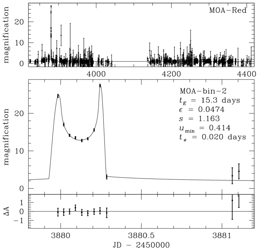
Figure 3: The light curve of event MOA-bin-2 in field gb19 with a $\sim 50\,$min sampling cadence. As in Fig. 1 top panel shows the 2006-2007 MOA-red data; the middle panel shows a close up of the light curve peak, and the bottom panel shows the residuals from the best fit. There are no OGLE data for this event.

Event MOA-bin-2 is located in field gb19, which had a $\sim 50\,$minute sampling cadence. The light curve, shown in Fig. 3, indicates a classic U-shaped caustic crossing shape spanning $\sim 7\,$hours, and like the case of MOA-bin-1, this is a light curve shape that is unique to microlensing. However, there is no light curve coverage during the 4 days prior to the caustic crossing. As a result, the model parameters are not very tightly constrained. The best fit model has a brown dwarf mass ratio, $q=\epsilon/(1-\epsilon)=0.0497$, and its other parameters are listed in Table 3. However, there is a planetary mass ratio model with $q=1.7\times 10^{-3}$ that is disfavored by $\Delta\chi^{2}=4.08$, so a planetary secondary is not strongly excluded.

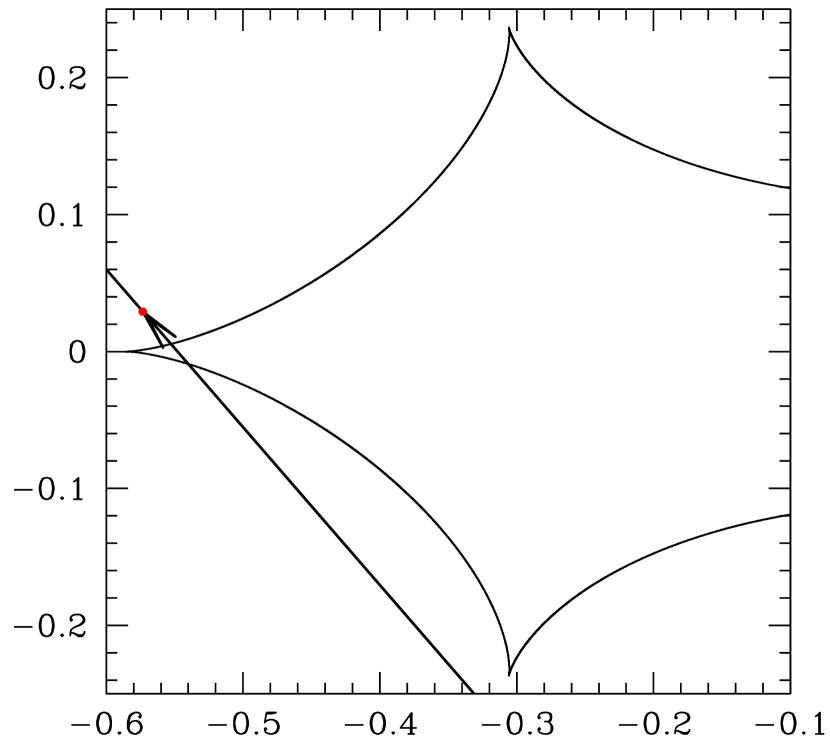
Figure 4: The caustic geometry for the best fit MOA-bin-2 model. As in Fig. 2, the red circle indicates the best fit source size, and the coordinates for this plot are centered at the center-of-mass of the full lens system.

The caustic configuration for the best fit model is shown in Fig. 4. This model has a connected or “resonant” caustic, while the planetary models cross the same cusp (the most distant one) of a separated planetary caustic.

3.3 MOA-bin-3

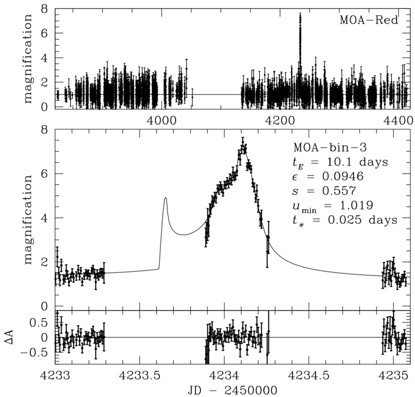
Figure 5: The light curve of event MOA-bin-3 in field gb5 with a $\sim 10\,$min sampling cadence. As in Fig. 1 top panel shows the 2006-2007 MOA-red-band data; the middle panel shows a close up of the light curve peak, and the bottom panel shows the residuals from the best fit. There are no OGLE data for this event.

Fig. 5 shows the light curve of MOA-bin-3, which is the only binary event in our sample with a separation $s<1$. A close separation binary is the one configuration in which a system of two stars can give rise to a very small caustic that is not surrounded by a region of high magnification. So, as discussed by Sumi et al. (2011), stellar binary lens systems with a separation $s\ll 1$, are the main microlensing background for the short duration single lens microlensing events, which were used by Sumi et al. (2011) to infer a new population of isolated planetary mass lenses.

In the case of MOA-bin-3, the preferred fit has a moderate separation of $s=0.557$, which means that the caustic crossed by the source (see Fig. 6) is not extremely small, with a width (along the source trajectory) of $\sim 0.05\,R_{E}$. But, the model compensates for this with duration of $\sim 10\,$days, which is about half the typical event duration.

The mass ratio for this event is $q=\epsilon/(1-\epsilon)=0.104$, which implies that the secondary is a brown dwarf in the (likely) case that the host star mass is $<0.77M_{\odot}$.

This event also has a wide separation model with $s=1.609$ and $q=7.7\times 10^{-3}$, but this model is disfavored by $\Delta\chi^{2}=19.7$. So, the close binary, brown dwarf secondary model is probably the correct one.

3.4 A Flare Star Fit by a Microlensing Model

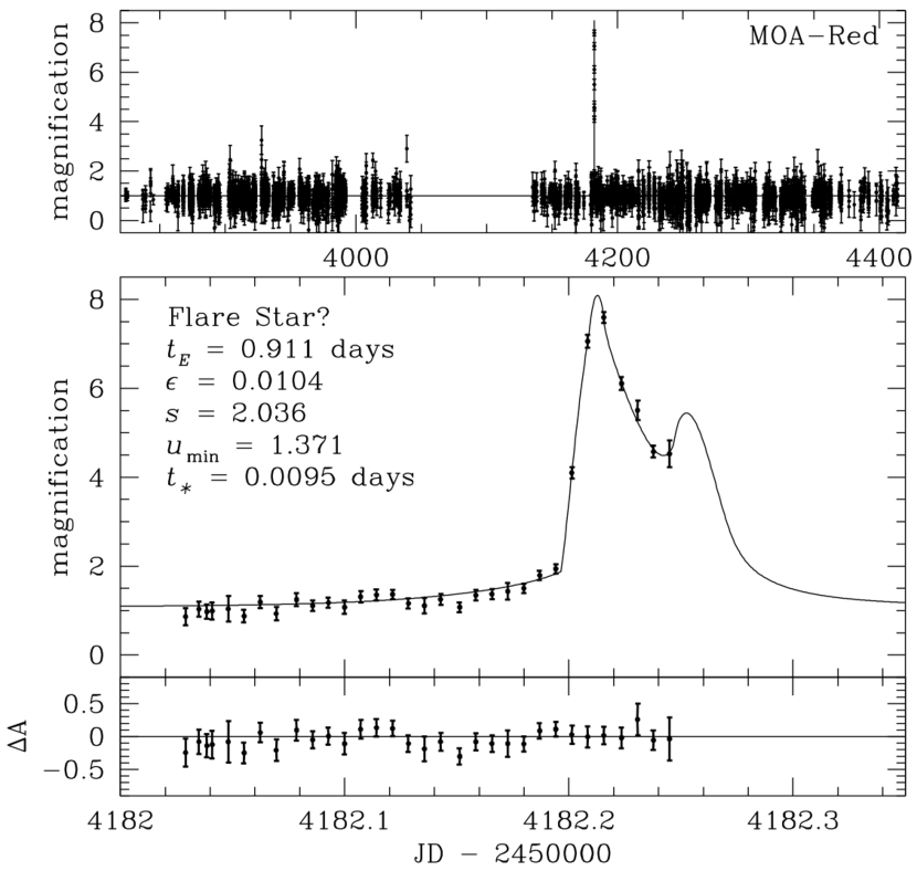
Figure 7: The light curve of an event that is well modeled by an extremely short binary lens light curve, with an Einstein radius crossing time of $t_{E}=0.911\,$days. The mass ratio is $q\approx 0.01$, which implies that if this model is correct, the lens system would likely be an isolated gas giant planet with a moon that has a mass similar to Earth. However, the light curve features are not oversampled, and a foreground late M-dwarf is located at the position of the event. This implies that the most likely interpretation is that this is a large amplitude M-dwarf flare (Kowalski et al., 2010).

Fig. 7 shows the light curve of the fourth event that is well fit by a very short binary lens light curve. If the microlensing model for this event was correct, it would be a remarkable discovery. The event timescale is so short, $t_{E}=0.911\,$days, that the primary lens is very likely to have a planetary mass, similar to the mass of Jupiter. Thus, the secondary, which is nearly 100 times smaller, would have a mass of a few Earth masses.

However, there are a number of reasons to be suspicious about this model. It predicts a typical main sequence source brightness of $I\sim 19.5$, but the source radius crossing time is quite small, $t_{\ast}=0.0095\,$days. If we assume a typical source radius of $\theta_{\ast}\sim 0.5\,$mas, then we have a source-lens relative proper motion of $\mu_{\rm rel}\sim 19\,$mas/yr. This compares to a typical relative proper motion of $\mu_{\rm rel}\sim 6\,$mas/yr, and it corresponds to a relative velocity of $\sim 700\,$km/s if both the source and lens are in the bulge. Most likely, it would indicate that lens is quite close to us, at a distance of $\lower 2.15277pt\hbox{$\;\buildrel<\over{\sim}\;$}1\,$kpc.

A worrying feature of this small $t_{\ast}$ value is that it means that the caustic crossing feature at $t\simeq 4182.2$ is not oversampled, despite the fact that this event is in high cadence field gb9, which has a 10 minute sampling cadence. This means that we cannot claim to have confirmed a unique microlensing feature for this event. In fact, there only 7 observations with fit magnification $A>2$, which compare to a total of 8 fit parameters: 5 binary lens fit parameters, 2 linear flux parameters (the source and blend fluxes), and $t_{\ast}$. While there are also 5-10 additional data points indicating a gentle rise just before the apparent caustic entry, the number of data points used to constrain the model is not much larger than the number of model parameters. So, the fact that the data fit the model does not provide convincing evidence that the model is correct. Furthermore, the caustic exit feature is not observed, and caustic entrance features tend to more closely resemble the light curves of eruptive variable stars, like CVs and stellar flares.

The OGLE-III photometry for this field (Szymański et al., 2011) indicates that the event is superimposed on a star with $I=17.8$ and $V-I=2.9$, with an apparent proper motion of $\sim 10\,$mas/yr. In the microlensing interpretation, this could be the average of the combined proper motion of the the $I\simeq 19.5$ source star and the brighter foreground star. The foreground star could not be the lens, but it could be a stellar host associated with the planetary mass primary lens. It would have to be $\lower 2.15277pt\hbox{$\;\buildrel>\over{\sim}\;$}10\,$AU from the lens to avoid detection.

Depending on the fraction of the total extinction to the bulge ($E(V-I)\simeq 0.75$ (Popowski et al., 2003)) that is in the foreground of this star, the observed color of this star would correspond to an M2-M4 dwarf. The observed brightening would correspond to $\sim 1\,$mag for this foreground star (since it is brighter than the “host” star implied by the light curve model). This means that a “mega-flare” (Kowalski et al., 2010) would be a possible explanation for this observed light curve. Studies of the frequencies of flares on “inactive” M2-M4 dwarfs indicate that a flare of this magnitude would be expected to occur about once every $\sim 10\,$years (Kowalski et al., 2009; Hilton et al., 2010; Hilton, 2011). Thus, the 2-year MOA-II survey of $\sim 50\,{\rm deg}^{2}$, should see many such mega-flares, and it is quite plausible that one such flare could be fit by a microlensing model. Thus, this is our preferred interpretation of this event.

If the microlensing interpretation was correct and the foregound M-dwarf is associated with the lens, there should be a $I\sim 19.5$ source star moving away from the foreground M-dwarf at a rate of $\mu_{\rm rel}\simeq 19\,$mas/yr. Since the microlensing event (if that is the correct interpretation) occurred in 2007, by 2012, the separation would be nearly $100\,$mas, so high resolution observations with HST (Bennett et al., 2006, 2007) or adaptive optics (AO) (Sumi et al., 2010; Bennett et al., 2010; Janczak et al., 2010; Kubas et al., 2012; Pietrukowicz et al., 2011) should be able to detect the source moving away from the foreground star.

This event illustrates the importance of a high sampling cadence, so that features that may be fit by a microlensing model are actually over-sampled. The over-sampling allows for much a much stronger test of the microlensing model as it will be much more difficult for the fitting code to adjust the parameters to match the light curve, unless the event is really due to microlensing. We also note that stellar variability, like flares, are much more likely to produce light curve that resemble caustic entrances than caustic exits.

4 The Physical Properties of MOA-bin-1LA, b

Many of the light curve parameters presented in Table 2 are given in units of the Einstein radius, $R_{E}=\sqrt{4GM_{L}D_{L}(D_{S}-D_{L})/(c^{2}D_{S})}$, where $M_{L}$ is the mass the lens system, and $D_{L}$ and $D_{S}$ are the masses of the lens and source, respectively. This means that the microlensing light curves can be modeled with a relatively small number of parameters, but it also means that the most well measured parameters of a microlensing event are measured in units of $R_{E}$, instead of physical units. In order to determine the physical parameters, it is very helpful to be able to measure the angular Einstein radius, $\theta_{E}=R_{E}/D_{L}$. In most planetary events, finite source effects are seen, so the source radius crossing time, $t_{*}$ can be measured. Since we can estimate the angular radius of the source star, $\theta_{*}$, from its brightness and color, it is usually possible to determine $\theta_{E}=\theta_{*}t_{E}/t_{*}$. For some planetary events (Bennett et al., 2008; Gaudi et al., 2008; Dong et al., 2009; Bennett et al., 2010; Muraki et al., 2011), it is possible to measure the projected Einstein radius, $\tilde{r}_{E}$, where the projection is from the lens position to the Solar System. This is known as the microlensing parallax effect (Gould, 1992; Alcock et al., 1995), and it is usually measured in long duration events, where the effect of the orbital motion of the Earth can be measured in the light curve. When this is measured, $M_{L}$ can be directly determined (Gould, 1992; Bennett, 2008; Gaudi, 2010),

$$M_{L}={c^{2}\over 4G}\tilde{r}_{E}\theta_{E}\ .$$ (1)

For the short duration events we present in this paper, there is no data that can be used to measure the microlensing parallax effect, so, we are left with the mass-distance relation,

$$M_{L}={c^{2}\over 4G}\theta_{E}^{2}{D_{S}D_{L}\over D_{S}-D_{L}}=0.9823\,M_{\odot}\left({\theta_{E}\over 1\,{\rm mas}}\right)^{2}\left({x\over 1-x}\right)\left({D_{S}\over 8\,{\rm kpc}}\right)\ ,$$ (2)

(where $x=D_{L}/D_{S}$) based on the measured value of $\theta_{E}$. In order to determine $\theta_{E}$, we must first work out the color and magnitude of the MOA-bin-1S source star. The magnitude in the non-standard MOA-red passband $R_{M}$ can be determined quite precisely from the observed light curve. The MOA-red source flux is determined from the best fit light curve, shown in Fig. 1 (with parameters listed in Table 2), and this can be compared to the standard Johnson $V$ and Cousins $I$ passbands by comparison to the OGLE-III photometry catalog (Szymański et al., 2011). This comparison yields

$$R_{M}=I+0.1485\left(V-I\right)\ ,$$ (3)

which differs somewhat from the transformation found by Gould et al. (2010a) for a comparison between the MOA-red passband and the OGLE-II photometry catalog. In principle, we could use eq. 3 as a color-color relation, $R_{M}-I=0.1485(V-I)$ to relate the measured $R_{M}-I$ photometry to $V-I$ as advocated by Gould et al. (2010a). (In Appendix B, we apply this method to five of the ten isolated planet events from Sumi et al. (2011).) As discussed in Section 3.1, for MOA-bin-1, there are no OGLE data at relatively high magnification, and they are not used in the fit due to concerns about blending-related systematic errors. Therefore, we estimate the source star color following the procedure of Bennett et al. (2008).

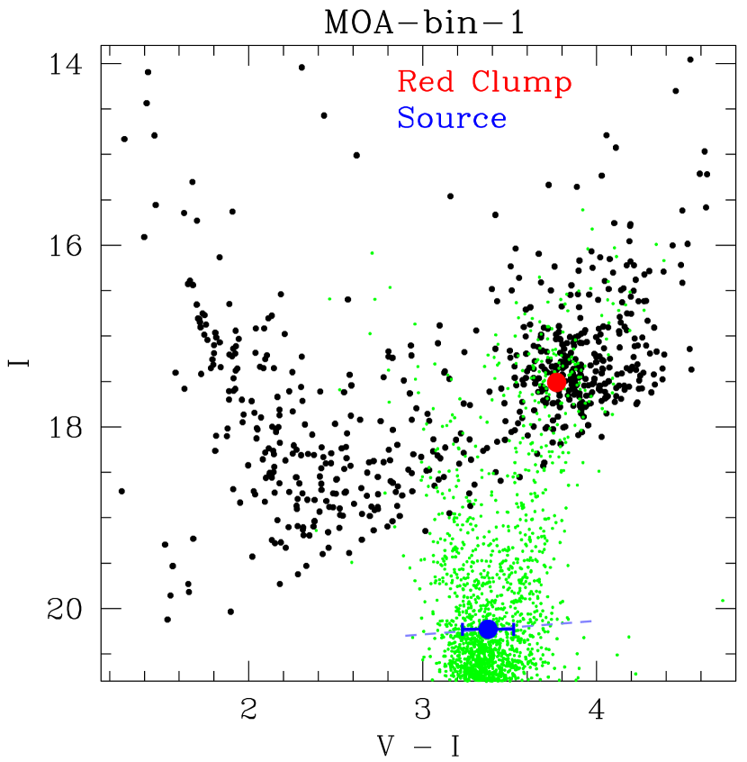
Figure 8: The color magnitude diagram (CMD) of the stars in the OGLE-III catlog within $60^{\prime\prime}$ of MOA-bin-1 is shown as black dots, while the green dots show the HST CMD of Holtzman et al. (1998), transformed to the same extinction (and extinction dispersion) as the field of MOA-bin-1. The red dot shows the centroid of the red clump giant distribution. The light blue dashed line shows the constraint based on the MOA-red source brightness of $R_{Ms}=20.73$, and the blue dot (and errorrbars) shows the source brightness $I_{s}=20.23\pm 0.02$ and color $(V-I)_{s}=3.38\pm 0.15$ estimated from a comparison with the HST CMD.

Fig. 8 shows the OGLE-III CMD (Szymański et al., 2011) of the stars within 1 arc minute of the MOA-bin-1S source star. The centroid of the red giant clump is located at $(V-I)_{\rm rc}=3.77$, $I_{\rm rc}=17.51$, which compares to the expected absolute magnitudes (Bennett et al., 2010) of $M_{I\rm rc}=-0.25$ and $M_{V\rm rc}-M_{I\rm rc}=1.04$. Since the event is located at a Galactic longitude of $l=-0.111^{\circ}$, we assume a distance of $D_{S}=8.0\,$kpc or a distance modulus of $DM=14.52$. This implies extinction of $A_{I}=3.24$, $A_{V}=5.97$, and $R_{VI}=A_{V}/(A_{V}-A_{I})=2.19$, since $A_{I}=I_{\rm rc}-M_{I\rm rc}-DM$ and $A_{V}=V_{\rm rc}-M_{V\rm rc}-DM$. This $R_{VI}$ value is quite typical of Galactic bulge fields (Udalski, 2003a), but the total extinction is much higher than is typical for the fields of observed microlensing events. The high extinction is also apparent from direct inspection of Fig. 8, as the OGLE catalog becomes highly incomplete (in the $V$-band) at less than 1 mag fainter than the red clump centroid.

We can estimate the source radius, following Bennett et al. (2008), by transforming the Baade’s Window CMD observed with HST by Holtzman et al. (1998) to the extinction and distance appropriate for the field of MOA-bin-1. When this is done, we find that there is considerably more scatter in the MOA-bin-1 CMD than in the HST Baade’s WIndow CMD. This is likely to be due to excess differential reddening in the MOA-bin-1 field. Therefore, we add a dispersion of 0.101 mag along the reddening line, and the resulting HST CMD is represented by the points shown in green in Fig. 8.

The best fit magnitude for the MOA-bin-1S source star is $R_{Ms}=20.73$ (see Table 2). As shown in Fig. 8, this is less than three $I$ mag fainter than the centroid of the red clump. This implies that the source could be a relatively young bulge main sequence star (Bensby et al., 2011), a turn-off star, or a sub-giant near the base of the giant branch. Comparison with the reddened HST CMD gives an $I$ magnitude of $I_{s}=20.23$ and a color of $(V-I)_{s}=3.38\pm 0.15$ for this particular model. The corresponding dereddened values are therefore $I_{s0}=16.99$ and $(V-I)_{s0}=0.65\pm 0.16$. The surface brightness-color relation of Kervella & Fouqué (2008) yields a source radius of $\theta_{*}=1.23\pm 0.18\,\mu$as, where the error bar only reflects the effect of the uncertainty in the source color. There is an additional uncertainty in the source radius due to the uncertainty in the source star brightness, but this is strongly correlated with the other event parameters. We account for this uncertainty separately in our Markov Chain Monte Carlo (MCMC) calculations, by adjusting the value of $\theta_{*}$ to account for the variations in the source brightness for each different set of model parameters. As indicated in Table 2, the outer cusp model has a best fit source magnitude of $R_{Ms}=20.75$, so these models predict a slightly smaller source, $\theta_{*}=1.21\,\mu$as. However, this solution also has shorter source radius crossing time, so the lens-source relative proper motion values for this solution is slightly larger, at $\mu_{\rm rel}=\theta_{*}/t_{*}=8.9\pm 1.4$ for the outer cusp solution than the value, $\mu_{\rm rel}=8.8\pm 1.4$ for the best fit model. These values are a little higher than the $\sim 6\,$mas/yr typical of bulge lensing events, but these $\mu_{\rm rel}$ are consistent with a lens system either in the disk or the bulge.

The implied angular Einstein radius values are $\theta_{E}=\theta_{*}t_{E}/t_{*}=0.77\pm 0.11\,$mas for the best fit (inner cusp crossing) model and $\theta_{E}=0.76\pm 0.11\,$mas for the best outer cusp crossing model. The effect of the larger $t_{E}$ and smaller $t_{*}$ compensate for the smaller $\theta_{*}$ for this model. These $\theta_{E}$ values can be used to constrain the mass of the lens system using eq. 2.

Alcock et al. (1997) present a method to use eq. 2 to make a Bayesian estimate the probability distribution of the distance, $D_{L}$, and mass, $M_{L}$, based on a Galactic model of the stellar kinematic and density distribution. We have supplemented this method by allowing the source distance, $D_{S}$, to vary, and used the Galactic model parameters from Bennett & Rhie (2002). This yields a probability table as a function of relative proper motion, $\mu_{\rm rel}$, source distance, $D_{S}$, and the lens system distance, $D_{L}$. This probability table is used as an input to a program that sums the MCMC likelihood results in order to properly weight the different light curve models with the probability of the parameters that they imply. This routine determines the probability distribution of the physical parameters, which depend on both the fit parameters and the unmeasured parameters $D_{L}$ and $D_{S}$. For the relative proper motion, $\mu_{\rm rel}$, which is measured, we use the galactic model weights to marginalize over the measurement uncertainty. For each model in the MCMC, we have a value of $t_{E}$, which can be combined with the relative proper motion to yield the angular Einstein radius, $\theta_{E}=\mu_{\rm rel}t_{E}$. This allows us to determine the lens mass using eq. 2, since we are marginalizing over $D_{L}$ and $D_{S}$. Once the lens mass is determined, we can apply a mass prior, using the power-law mass function of Sumi et al. (2011). (This is mass function # 3 presented in the Supplementary Information.) The advantage of this mass function is that it includes possible brown dwarf and even planetary mass hosts, which could plausibly host a planetary mass ratio companion.

The results of these MCMC calculations are summarized in Table 4, which gives the median values and $1\,\sigma$ and $2\,\sigma$ confidence level limits on the planetary system distance, $D_{L}$, host star mass, $M_{*}$, planet mass, $m_{p}$, and the semi-major axis, $a$. Both the OGLE and MOA data indicate that the MOA-bin-1 source star is blended with a star with an $I$ magnitude of $I_{b}=19.66$, which can be used as an upper limit on the source brightness. Due to the high dust extinction in this field, however, this constraint does not exclude host stars less massive than $1\,M_{\odot}$. The bulge turn-off mass is $\sim M_{\odot}$, but there are some young stars in the bulge (Bensby et al., 2011). In order to avoid excluding these possible host stars with an a priori assumption, we have modified the Sumi et al. (2011) mass function # 3 by adding a population of such stars with a mass function that scales like $dN/dM\propto M^{-4}$ for $M>1\,M_{\odot}$.

Table 4 indicates the host star is most likely to be a an late K-dwarf, but the $2\,\sigma$ range spans virtually the entire main sequence available in the bulge. The planet is quite massive, at $m_{p}=3.7\pm 2.1\,M_{\rm Jup}$, probably the most massive planet yet found by microlensing. It may also be the widest separation planet found by microlensing, although one of the two degenerate solutions for MOA-2007-BLG-400Lb (Dong et al., 2009b) does have a wider separation.

Previous microlensing work has shown that sub-Jupiter-mass gas giants are rather common in orbit around M-dwarfs (Gould et al., 2010b), and has also found several cases of super-Jupiter-mass planets orbiting M-dwarfs Udalski et al. (2005); Dong et al. (2009); Batista et al. (2011). In contrast, radial velocity studies (Johnson et al., 2007; Bonfils et al., 2011) have found a low occurrence rate of super-Jupiter-mass planets orbiting M-dwarfs. However, most of the radial velocity sensitivity is to planets in shorter period orbits than the microlensing discoveries, so it is not clear that there is a discrepancy between these results. The core accretion theory does seem to predict that only a small fraction of M-dwarfs will have massive gas-giant planets (Laughlin et al., 2004; Ida & Lin, 2005; Kennedy & Kenyon, 2008; D’Angelo et al., 2010), so If the MOA-bin-1Lb planet and its host have the median predicted masses, then this might suggest that this planet formed by gravitational instability (Boss, 2006) instead of core accretion. However, the error bars on the MOA-bin-1L host star mass are quite large, so a solar-type host is also possible.

The uncertainty in the host star properties can be resolved with HST follow-up observations, which should be able to detect the host star if it has a mass of $\lower 2.15277pt\hbox{$\;\buildrel>\over{\sim}\;$}0.4M_{\odot}$ using the color dependent centroid shift (Bennett et al., 2006; Dong et al., 2009) or the image elongation (Bennett et al., 2007) methods. These methods should be able to detect the host star at current separation of $\sim 50\,$mas assuming a mass of $\lower 2.15277pt\hbox{$\;\buildrel>\over{\sim}\;$}0.4M_{\odot}$. It may also be possible to detect the host star with AO infrared imaging (Bennett et al., 2010; Sumi et al., 2010; Janczak et al., 2010; Kubas et al., 2012), since a diffraction limited image could resolve the source and planet host stars. However, since we have no infrared imaging while the event was in progress, there is some potential that IR images may not be able to distinguish the source and planet host stars. But, assuming that we do not have this problem, the follow-up observations would also be able to provide a measurement of the source star color, which would improve our estimate of $\theta_{*}$ and allow the determination of the host star mass using eq. 2 and a mass-luminosity relation as discussed in Bennett et al. (2006, 2007).

5 Implications for Planets in Wide Orbits

The bona fide planetary event, MOA-bin-1, is an example of a previously unseen type of planetary microlensing event - an event nearly in the Chang-Refsdal limit (Chang & Refsdal, 1979, 1984), where the main effect of the host star is to create the planetary caustic. In order to establish the precise statistical implications of the discovery such events, we should calculate their detection efficiency. We haven’t done this, but a detailed consideration of the MOA-bin-1 allows us to make a rough estimate of the detection efficiency for such events. The green dashed curve in Figure 1 indicates that the magnification due to the host star alone is so small, $A_{\rm max}=1.10$, that the event would be undetectable, without the planet. (The source is blended with another star that is a magnitude brighter, so the apparent peak magnification is only $A_{\rm max}\sim 1.03$.) If the planet was isolated, without a host star, it would generate the light curve indicated by the blue-dashed curve in Figure 1, which has a peak magnification of $A_{\rm max}=2.58$. This is high enough so that the event would have still been detected in the short timescale analysis of Sumi et al. (2011), but it is much smaller than the observed peak magnification of $A_{\rm max}=19.1$.

This illustrates why the detection efficiency for Chang-Refsdal-like events is likely to be higher than for single lens events with the equivalent effective parameters. For MOA-bin-1, the observed light curve is much brighter than the equivalent single lens light curve. This is a generic situation because the caustics of Chang-Refsdal-like lens systems spread the region of relatively high magnification ($A\lower 2.15277pt\hbox{$\;\buildrel>\over{\sim}\;$}10$) over larger area than for the equivalent single lens events. The area of extremely high magnification $A\lower 2.15277pt\hbox{$\;\buildrel>\over{\sim}\;$}100$ is reduced, but this is likely to affect the detection efficiency less than the larger area at $A\lower 2.15277pt\hbox{$\;\buildrel>\over{\sim}\;$}10$. One might also worry that our subjective procedure to select binary events from the low-level event candidates of the Sumi et al. (2011) sample could have missed some events, but we feel that this is unlikely since we have modeled all the events that remotely resemble short duration binary lens events.

With the assumption that the detection efficiency for Chang-Refsdal-like events is higher than for single lens events, we can combine the results of this paper with those of Sumi et al. (2011) to determine properties of the semi-major axis distribution of this newly discovered planet population, assuming that they are in very distant orbits about their host stars. We have found only one Chang-Refsdal-like event that is a bona fide microlensing event due to a planetary mass lens, MOA-bin-1. However, the effective timescale of this event is actually too large to qualify for the Sumi et al. (2011) sample. If we take away the planetary host star for this event, then the planet-only Einstein radius crossing time becomes $t_{Ep}=\sqrt{\epsilon}t_{E}=2.20\,$days, which is above the Sumi et al. (2011) cut of $t_{E}<2\,$days. Thus, the selection criteria which yield 10 isolated planetary mass microlenses find no planets at very wide separations with $s\geq 2$. (Note that MOA-2007-BLG-400 (Dong et al., 2009b) is an event in this sample, and it has a planet which may be in a very wide or a very close orbit, but the planetary signal was not seen in the MOA data and would not have been seen without the high magnification due to its host star.)

We can now use this result in combination with the lower limits on the separations of possible host stars for the 10 short single lens events of Sumi et al. (2011) to determine the properties of the planet separation distribution, under the assumption that these 10 isolated planetary mass objects are actually bound in distant orbits around stars. The lower limits on the separations of the 10 events with $t_{E}<2\,$days are listed in Table 1 of Sumi et al. (2011), and they are $s>7.0$, 3.3, 3.6, 3.1, 2.4, 4.8, 5.2, 4.8, 3.4, and 15.0 for events MOA-ip-1 through 10, respectively. These are measured in units of the Einstein radius of the possible host star. We can now use these lower limits to compare to possible distributions of wide separation planets to the data. We chose a very simple model,

$${dN\over ds}\propto s^{n}\ \ \ {\rm for}\ \ s_{0}<s<s_{1}\ ,$$ (4)

where the number of planets as a function of separation scales as a power law between inner and outer limits, $s_{0}$ and $s_{1}$. To conform with the limits from Sumi et al. (2011), these limits are all taken to be in units of the Einstein radius, $R_{E}$, of the possible host star. We select a lower separation limit of $s_{0}=2$, as this guarantees that star itself will not have a strong microlensing effect, so that the detection efficiency calculations of Sumi et al. (2011) will be applicable instead of the very different calculations needed to determine the detection efficiency to find planetary signals in events where the magnification of the host star dominates (Gould et al., 2010b; Cassan et al., 2012).

Perhaps, the most reasonable guess for $n$ in equation 4 would be $n=-1$, so that there is an equal probability of finding a planet in a logarithmic interval (between $s_{0}$ and $s_{1}$). This is the integer value of $n$ that is most compatible with observations, and it is the only integer value consistent with planets at a wide range of separations. Also, since the binding energy of the planet to its host star scales as $s^{-1}$, this is the choice that allows the the highest density of planets in stable orbits. With the selections, $n=-1$ and $s_{0}=2$, we now only need to specify $s_{1}$ in order to work out the probability that some number of the 10 (assumed bound) planets will have their host stars detected in the Sumi et al. (2011) microlensing data. With these values selected, it is then trivial to simulate $10^{6}$ simulations of the Sumi et al. (2011) 10-event sample and determine what fraction of these simulated observations reproduce the observed number of 0 out of 10 detectable host stars. Since, we seek to set a limit on the planetary distribution to be consistent with the observations, we select $s_{1}$ values that will yield a probability of 5% or 10% to detect 0/10 host stars. As shown in Table 5, $s_{1}=60$ yields a probability of $P(0/10)\simeq 5\,$%, and $s_{1}=135$ yields a probability $P(0/10)\simeq 10\,$%. So, these planet separation distributions represent the 95% and 90% confidence levels with our assumptions on the form of the planet separation distribution and that all planets are bound.

One possible objection to this choice of $n=-1$ is that the abundance of isolated planets found by Sumi et al. (2011), $1.8{+1.7\atop-0.8}$ per main sequence star, is somewhat larger than expected. So, perhaps, we should consider a distribution with more outer planets than we would expect. Another choice that would put more planets in outer orbits is $n=0$, a uniform distribution is separation instead of in the logarithm of the separation. This choice is shown in the last two columns of Table 5. Since these distributions are more heavily weighted toward outer planets, the $s_{1}$ values corresponding to the 95% and 90% confidence level limits are much smaller, at $s_{1}=18$ and 21, respectively.

While the outer cutoffs for these $n=-1$ and $n=0$ distributions are quite different at the 95% or 90% confidence levels, the median values of these distributions (equation 4) are much closer. For 95% confidence, at $n=-1$, we have $s_{1}=60$, which implies a median of $s_{m}=11.0$. At $n=0$, the 95% confidence value for $s_{1}=18$, which gives a median of $s_{m}=10.0$. At 90% confidence, the $s_{1}$ values are 135 and 21 for the $n=-1$ and $n=0$ models, respectively, and these give median values of $s_{m}=16.4$ for $n=-1$ and $s_{m}=12.5$ for $n=0$.

Now, for a typical lens star, a two-dimensional separation of an Einstein radius ($s=1$) corresponds to an orbital semi-major axis of $\sim 3\,$AU. Thus, the 95% confidence limit of $s_{m}>10.0$ from the $n=0$ model implies that a distribution of bound planets that could explain the Sumi et al. (2011) results if it had a median semi-major axis of $a_{m}>30\,$AU. With the $n=-1$ model, the limit would be slightly stronger, $a_{m}>33\,$AU. While we have only considered a couple of simple models for the separation distribution of planets in wide orbits, the models that we do consider do bound the power-law models that best match the observed distributions of exoplanets (Cumming et al., 2008; Cassan et al., 2012). Thus, it seems likely that a substantial fraction of the Sumi et al. (2011) population of isolated planets must be unbound or in orbits beyond $30\,$AU.

6 Summary and Conclusions

In this paper, we have presented the analysis of 4 events from the MOA Project’s 2006-2007 short event analysis, which were well-fit by binary lens light curve models. Two of these events, have best fit binary microlensing models, in which the signal is dominated by a planetary mass secondary with a distant primary that affects the light curve primarily through the gradient of its gravitational field, but we do not consider them both to be bona fide microlensing events. One of these events, MOA-bin-1, has a an oversampled, characteristic cusp-crossing feature, which makes it obvious that the microlensing interpretation is correct. The other event with a best fit planetary mass microlensing light curve has an apparent caustic crossing feature that is much more rapid than for typical microlensing events, and as a result, the feature is only marginally sampled by the high cadence MOA images. The number of observations that are much brighter than the baseline brightness is not much higher than the number of model parameters needed to describe them, so the fact that the light curve is well fit by a microlensing model does not imply that the model is likely to be correct. Furthermore, it is located at the position of a foreground M-dwarf that is expected to have a “mega-flare” of a similar magnitude about once every ten years. This is much higher than the expected lensing rate, so we have concluded that this event is unlikely to be a microlensing event. This event illustrates the importance of oversampling the microlensing features in the light curve. Oversampling implies that there are many more data points on the light curve features than there are model parameters that can be adjusted to fit the data. This allows the additional data points to be used to establish the microlensing nature of the event, as occurs for MOA-bin-1 (and to some extent for MOA-bin-2).

We have also done a preliminary investigation of the implications of the search for Chang-Refsdal-like planetary events, using a rather crude estimate of the detection efficiency for our somewhat subjective event selection procedure. In particular, we have assumed that the detection efficiency for such events is not smaller than the detection efficiency for the equivalent short single lens events. The arguments given in Section 5 indicate that this is likely to be the case, but this has not been directly demonstrated. If all of the isolated planetary mass microlensing events found by Sumi et al. (2011) were due to bound planets with a simple power-law distribution, we find that the median star-planet separation must be $\lower 2.15277pt\hbox{$\;\buildrel>\over{\sim}\;$}30\,$AU.

We plan a more detailed analysis of this question in a future paper with three times larger sample of events, and with a detailed analysis of the detection efficiencies. We expect that this analysis will provide a significantly stronger limit than we have presented here for a couple reasons. First, here we have assumed that the detection efficiency for the wide separation planets is the same as for isolated planets, but in fact, for events like MOA-bin-1, the detection efficiency for the wide separation planets is likely to be higher. So, the failure to detect any wide orbit planets with $t_{Ep}<2\,$days is likely to be more significant than we have assumed. Second, a much larger sample of short duration microlensing events with $t_{E}<2\,$days has been obtained in the years since 2007 with the MOA-II alert system (Bond et al., 2001) and the OGLE-IV Early Warning System (Udalski et al., 1994), but no other examples of wide separation planets, beyond MOA-bin-1 (with $t_{Ep}=2.2\,$days) have been seen. This suggests a more rigorous future analysis using calculated wide-planet detection efficiencies and the full sample of 2006-2012 MOA-II and 2010-2012 OGLE-IV data should a much more stringent lower limit on the median semi-major axis of these isolated planetary mass lenses, unless other wide separation planet events have been missed.

Finally, an alternative method to probe the possibility of host stars for the isolated planets of Sumi et al. (2011) is with follow-up HST imaging of the current sample of $\sim 30$ such events, plus a similar size sample of events with $2\,{\rm days}<t_{E}<4\,$days. While the events with $t_{E}<2\,$days are thought to be mostly due to planets, most of the events with $t_{E}\sim 3$ or 4 days are likely to be due to brown dwarfs. If a substantial fraction of the isolated planet population has host stars, then 50% or more of the host stars should be detectable in HST images, and multiple epoch HST imaging can confirm that the candidate host stars have proper motions consistent with our expectations for host stars using the methods of Bennett et al. (2006, 2007). On the other hand, we would expect that almost all of the brown dwarf lenses should not have host stars, due to the brown dwarf desert. So, HST observations of $t_{E}\sim 3$ and 4 day events should not reveal host stars. (A few events may be due to high proper motion stars, but these are readily identified with multiple HST frames.) The combination of HST observations with the analysis of the post-2007 microlensing data should teach us a great deal about the nature of this newly discovered isolated planet population.

Appendix A Non-planetary Models for MOA-bin-1

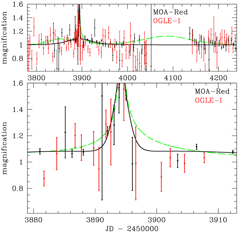
Figure 9: Comparison of planetary (black) and non-planetary (green dashed) light curve models for event MOA-bin-1. The MOA and OGLE data are binned with different bin sizes depending on the time difference from the cusp crossing peak. There is no binning within 12 hours from the peak. Between 0.5 and 4.5 days, the data are binned in 1-day bins, and between 4.5 and 10.5 days, 2-day bins are used. The remaining data is binned in in 5-day bins.

As discussed in Section 3.1, there are are non-planetary models for MOA-bin-1 that can describe the cusp crossing feature but are excluded by the observations of the light curve outside of the cusp crossing peak. These solutions have a similar caustic structure to the best solution, indicated in Fig. 2, but the source crosses the top or bottom cusp instead of the inner or outer one. Because these solutions involve source motion that is nearly parallel to the lens axis, they are likely to have additional peaks due to a close passage to the cusp associated with the other mass (in this case, the primary mass). However, because of the near Chang-Refsdal nature of the light curve, there are only weak constraints on the location and strength of such a peak in the light curve. This allows such a feature to be attracted to systematic error features that might exist in the light curve. As mentioned in Section 3.1 and shown in Figure 9, the non-planetary solution for MOA-bin-1 gets a $\Delta\chi^{2}=16.3$ improvement from data in late-February, early-March, 2007 ($t\sim 4165$).

We believe that this feature at $t\sim 4165$ is likely to be due to a systematic photometry error. As discussed in Section 2.1, the MOA photometry for MOA-bin-1 shows evidence of a systematic error related to the direction and amplitude of differential refraction. Our empirical correction of this effect has reduced the significance of this apparent feature from $\Delta\chi^{2}\sim 95$ to $\Delta\chi^{2}=16.3$. It seems likely that the remaining improvement could be due to an imperfect correction.

One obvious way to check the possibility that this feature is due to a systematic error in the MOA data is to compare to the OGLE data. However, as mentioned in Section 3.1, there is also a systematic error that affects the OGLE data. OGLE uses an implementation of difference imaging (Udalski, 2003b) with photometry done at the centroid of stars identified in the reference frame. But, because the central Galactic bulge fields are very crowded, the faint stars identified in the OGLE frames are typically blends of several stars, so the centroids of the identified stars do not line up with the actual position of the faint source stars. Often, the photometry can be significantly improved by identifying source star position from the centroid in a good seeing difference image, taken when the source is highly magnified. Unfortunately, the source is not seen at very high magnification in the OGLE data, and the three OGLE data points at moderate magnification of $A\sim 1.7$ where taken in poor seeing. So, identification of the optimal centroid of the source in the OGLE data is difficult, and this is probably why optimum centroid photometry of the OGLE data is not available.

Without the optimum centroid photometry, there are two choices for dealing with the OGLE photometry. The simplest choice is to to simply fit the OGLE data as an independent data set. This gives the results that were reported in Section 3.1. However, we can use the methods described in Appendix B to work out the source color implied by these models, and these indicate unreasonably blue source colors. For the best fit model, with a crossing of the outer cusp of a planetary mass secondary, this gives $(V-I)_{s}=-0.1\pm 1.2$, while for the best fit upper or lower cusp crossing model (with a non-planetary mass ratio) the implied color is $(V-I)_{s}=-4.1\pm 1.4$. As shown in Figure 8 and discussed in Section 4, the real source color is $(V-I)_{s}=3.38\pm 0.15$, which is 2.9-$\sigma$ redder than the best fit (planetary) model and 5.3-$\sigma$ redder than the best upper or lower cusp crossing (non-planetary) model. These unreasonable colors are an indication of a problem with the OGLE photometry centroid.

If we require that the source brightness in the OGLE $I$-band be consistent with a normal source star (i.e. with $(V-I)_{s}=3.38\pm 0.15$), we find that $\chi^{2}$ is increased by $\Delta\chi^{2}=7.9$ for 2373 OGLE $I$-band observations. This is another indication that the systematic error driving the source color toward an unreasonably blue value is just under a 3-$\sigma$ effect.

Since we know that a normal source star must have a color of $(V-I)_{s}=3.38\pm 0.15$, it is sensible to enforce such a constraint on the different models for MOA-bin-1. Because the non-planetary, upper and lower cusp crossing models predict a source color that is too blue by more than 5-$\sigma$, we should expect that these non-planetary models should be disfavored by the requirement that the lensed source have a reasonable stellar color, and this is indeed the case. The $\chi^{2}$ difference between the best fit model and the best fit upper or lower cusp crossing model increases from $\Delta\chi^{2}=17.5$ to $\Delta\chi^{2}=54.4$. The lower magnification part of these two models are shown in Figure 9, with the best fit model shown in black and the best upper or lower cusp crossing model shown as a dashed green curve. The data shown in this Figure is binned for clarity, but all the fits are done with the original unbinned data.

The parameters for the best fit planetary model with this constraint are somewhat different from the values listed in Table 2. With this constraint, the best fit has $t_{E}=22.5\,$days, $t_{0}=3894.4$, $u_{\rm min}=1.659$, $\theta=1.565$, $\epsilon=0.0078$, $t_{\ast}=0.0489\,$days, and $R_{M}=20.65$. The best fit upper or lower cusp crossing (non-planetary) model has $t_{E}=147.3\,$days, $t_{0}=4042.5$, $u_{\rm min}=-0.434$, $\theta=6.044$, $\epsilon=0.162$, $t_{\ast}=0.0519\,$days, and $R_{M}=22.74$. These are the models shown in Figure 9. This figure indicates that the best fit model is favored at $3885<t<3905$ because the non-planetary model predicts higher magnification in the wings of the peak. But, in the beginning of the 2007 season at $4135<t<4200$, the non-planetary, upper or lower cusp model is favored in the MOA data, but not the OGLE data. If these data are excluded, then the difference between the best fit model (planetary) model increases to $\Delta\chi^{2}=73.4$. We regard this, and all other, non-planetary models as being excluded by the data.

Appendix B Short Event Source Star Colors

In this Appendix (B), we compare the photometry of the short events of Sumi et al. (2011) plus the binary events presented in this paper to the OGLE-III photometry catalog in order to determine calibrated source magnitudes and colors. Gould et al. (2010a) have argued that color of microlensed source stars observed by both MOA and OGLE can be determined from the differences between the MOA-Red passband and the OGLE-$I$ passband, which is similar to the standard Kron/Cousins $I$-band. Since the MOA-Red band is essentially equivalent to the sum of the standard Kron/Cousins $R$ and $I$-bands, the color difference between the MOA-Red and OGLE-$I$ is rather small, and this implies that the source brightness must be measured quite precisely in both passbands in order to obtain a $V-I$ color of reasonable precision. This is an important difficulty with the present analysis because the events presented here and in Sumi et al. (2011) have brief periods of magnification and because the OGLE survey involved is the relatively low-cadence OGLE-III survey. The higher cadence of the current OGLE-IV survey will help to alleviate this problem. As discussed in Section 4, it was the low precision of the OGLE-III source flux measurement that caused this method to fail for MOA-bin-1. This is also the reason why this method fails for events MOA-ip-6, and 8 from Sumi et al. (2011). This method also cannot be used for MOA-ip-1, 5, and 10, because there is no OGLE-III data during these events. Thus, we can only present color measurements for the MOA-ip-2, 3, 4, 7 and 9 source stars in this paper. For MOA-bin-1, MOA-bin-3 and the remaining Sumi et al. (2011) events, we determine the transformation between the MOA and OGLE-III magnitude systems, but we can only estimate the source color with a comparison to HST photometry. Event MOA-bin-3 does not lie in any OGLE-III field, so it is not included in this analysis.

As discussed in Section 2, the state of the art method for crowded field photometry of time-varying sources is difference image analysis (DIA) photometry. However, this method does not provide photometry for the bright, relatively isolated stars that are needed to determine the transformations between the passbands used for the observations and standard passbands. Photometry of these stars must be done with a point-spread function (PSF) fitting routine, such as DoPHOT (Schechter, Mateo, & Saha, 1993). As explained by Gould et al. (2010a), there are substantial differences in the way photometry is done with the DIA and PSF fitting methods, and so there is an additional step to determine the magnitude offset between the PSF fitting and DIA photometry of the same images. This was done comparing the PSF fitting photometry of apparently isolated stars to photometry done using an internal DIA PSF fitting photometry algorithm. This later algorithm has no way to handle blending. So, if too few sufficiently isolated stars can be found, it will be impossible to get accurate photometry of the field stars using the DIA fitting method. Of course, this entire method also depends on PSF fitting photometry for the comparison of bright stars, but this is the situation that PSF fitting photometry codes were designed to handle: the photometry of stars in relatively crowded stellar fields. So, this attempt to use the DIA PSF fitting routine on unsubtracted images could be a major weakness of the Gould et al. (2010a) method.

We introduce a new method that does away with the need to find stars that are so isolated that good photometry can be done with the DIA PSF fitting method, which is designed for uncrowded, subtracted frames. The PSF fitting method for a crowded field PSF-fitting photometry code, like DoPHOT (Schechter, Mateo, & Saha, 1993) or SoDoPHOT (Bennett et al., 1993) should also work for uncrowded difference images, so this is what we do. We use the MOA DIA pipeline (Bond et al., 2001) for the difference image photometry and use both the registered, unsubstracted frames and difference images from the MOA pipeline as input for a custom version of SoDoPHOT. The MOA DIA pipeline first generates registered frames, which are transformed (and resampled) to have the same astrometry as the reference image. Then the reference image is convolved to the seeing of the registered image, and it is subtracted from the registered image to give the difference image. The result is that we have two sets of images, the registered images and the difference images, with the same photometric scaling and the same PSF shape. The registered frame has all the information of the stellar brightnesses from the original image, while the difference images have only the difference in flux from the reference frame.

We then feed both the registered and difference images into our custom version of SoDoPHOT. The registered frames are processed as normal images, but the PSF model from each registered frame is also used to do photometry on the target star in the difference image. The result is a normal time series of SoDoPHOT photometry from the registered frames plus photometry from the difference images using the SoDoPHOT PSF model on the same photometric scale as the as the PSF fitting photometry from SoDoPHOT. Thus, we automatically have PSF and DIA photometry on the same photometric scale. The SoDoPHOT generated DIA photometry may be slightly worse than the DIA photometry generated directly from the MOA pipeline, but in the examples presented here, we have found that both types of photometry in these difference images were nearly identical. The light curves presented in this paper use the original MOA pipeline DIA photometry, while the color measurements discussed below use SoDoPHOT PSF version of this photometry.

Now, in order to determine the color of the source stars for 5 of the 10 microlensing events with $t_{E}<2\,$days from Sumi et al. (2011), we must consider three types of photometry:

• The OGLE-III catalog photometry, transformed to the standard Kron/Cousins $I$-band and the Johnson $V$-band (denoted by $I$ and $V$) (Szymański et al., 2011).

• MOA-II photometry in the MOA-Red banded, denoted by $R_{M}$.

• OGLE-III photometry in the native OGLE $I$-band, denoted by $I_{O}$.

The $R_{M}$ and $I_{O}$ magnitudes of the source ($R_{Ms}$ and $I_{Os}$) are determined from the microlensing light curve fits to the joint MOA and OGLE data sets. These magnitudes are indicated in Table B1. Note that the error bars in the source magnitudes in this table assume that the parameters of the microlensing model are fixed at the best fit values, but they do not include any effect of light curve model uncertainties.

As discussed in Szymański et al. (2011), the relationship between the native $I_{O}$ passband is non-linear due some transparency in the OGLE-III $I_{O}$-band filter beyond the wavelength range of the standard Cousins $I$-band. This relation is

$$I=I_{O}-d+\left(b_{\rm CCD}+g\right)\left(V-I\right)+h\left(V-I\right)^{2}\ ,$$ (B1)

where $d=0.033918$, $g=0.016361$ and $h=0.004167$. The parameter $b_{\rm CCD}\sim 0.04$ is necessary because of the slight variations in sensitivity as a function of wavelength for the eight different CCD chips in the OGLE-III camera (Udalski, 2003b).

In order to extract standard color information from the $R_{M}-I_{O}$ data available from the light curves we need an expression relating $R_{M}$ to the standard Johnson-$V$ and Cousins-$I$ bands. This is accomplished with a comparison of SoDoPHOT photometry of the field of each MOA event to the same field in the OGLE-III catalog. As discussed by Gould et al. (2010a), it is important to ensure that comparison stars do not have close neighbors in the OGLE catalog because the MOA images do not have seeing as good as the images used to construct the OGLE-III photometry catalog.

For the purpose of this analysis, we limit this MOA-OGLE color comparison to stars with colors slightly bluer than the top of the bulge main sequence to a few $\times 0.1\,$mag redder than the red clump, as this covers the range of plausible source star colors. This allows us to use a linear relation of the form

$$R_{M}=I+f\left(V-I\right)\ ,$$ (B2)

where the coefficient $f\sim 0.2$ depends on the particular field. (This field dependence is probably due to the width of the $R_{M}$ passband and the wide variation of interstellar extinction in the foreground of the Galactic bulge fields.

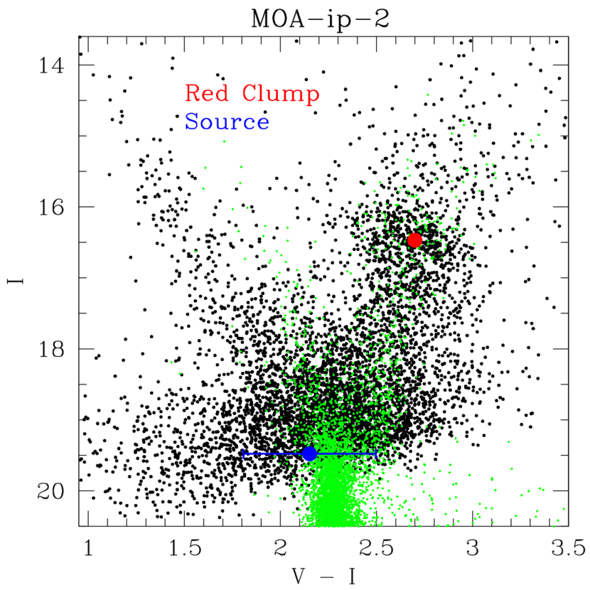
Figure 10: The CMD of the stars in the OGLE-III catlog within $120^{\prime\prime}$ of MOA-ip-2 is shown as black dots, while the green dots show the HST CMD of Holtzman et al. (1998), transformed to the same extinction as the field of MOA-ip-2. The centroid of the red clump is shown as a red dot, and the $I$ magnitude and color of the source star are shown in blue.

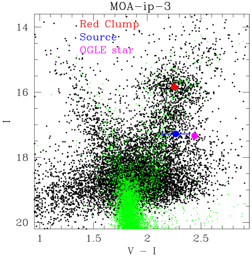
Figure 11: The CMD of the stars in the OGLE-III catlog within $120^{\prime\prime}$ of MOA-ip-3 are shown as black dots, and the green dots show the HST CMD of Holtzman et al. (1998), transformed to the same extinction as the field of MOA-ip-3. The centroid of the red clump is shown as a red dot; $I$ magnitude and color of the source star are shown in blue, and the with the color and magnitude of the star in the OGLE-III catalog located at the position of the event is shown as a magenta dot.

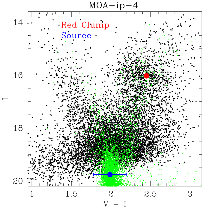
Figure 12: The CMD of the stars in the OGLE-III catlog within $120^{\prime\prime}$ of MOA-ip-4. The catalog stars, HST stars, red clump centroid and source star are indicated as in Figure 10.

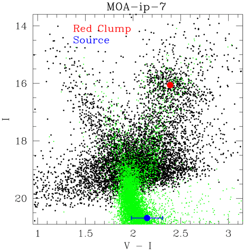
Figure 13: The CMD of the stars in the OGLE-III catlog within $120^{\prime\prime}$ of MOA-ip-7. The catalog stars, HST stars, red clump centroid and source star are indicated as in Figure 10.

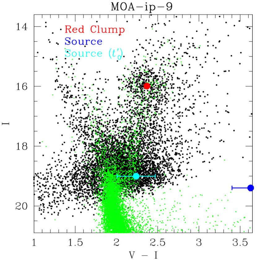
Figure 14: The CMD of the stars in the OGLE-III catlog within $120^{\prime\prime}$ of MOA-ip-9. The catalog stars, HST stars, red clump centroid and source star are indicated as in Figure 10. The cyan dot indicates the location of the source with a different $t_{0}$, which changes the color estimate to one is consistent with a bulge sub-giant source. This solution is disfavored by $\Delta\chi^{2}=2.36$.

The results of this analysis, as well as the adopted $b_{\rm CCD}$ and $f$ parameters given in Table B1 for events MOA-ip-2, 3, 5, 7 and 9. Figures 10-14 display CMDs for all the stars within 2 arc min of each event, as well as the locations of the adopted red clump centroid and the magnitude and color of the source star, which has been determined by this analysis. As in Figure 8, we also display HST bulge CMD from Holtzman et al. (1998) as green points, and we have aligned the HST CMD to the OGLE-III CMD by matching the red clump centroid appropriate for the Holtzman Baade’s Window field to the observed red clump position in the field of each event. But, unlike Figure 8, we do not broaden the CMD in an attempt to simulate the excess differential extinction in these fields compared to the Baade’s window.

The results for MOA-ip-2, 4, and 7 are similar. In each case, we find a source brightness and color consistent with a main sequence source star. For MOA-ip-2, the source is close to the main sequence turn-off, while the source for MOA-ip-4 and 7 are fainter, with the MOA-ip-7 source about 1.5 mag below the turn-off. All three of these sources are basically below the crowding limit in the OGLE-III catalog, so we cannot expect to identify the sources in images with $\sim 1^{\prime\prime}$ seeing.

The one source that does appear to be identified in the OGLE-III catalog is MOA-ip-3, and we indicate the CMD position of the apparent source as a magenta dot in Figure 11. The microlensing fit indicates that the source is in the middle of the sub-giant branch of the CMD about half-way between the base and the red clump. It is not surprising that the source appears to be on the sub-giant branch, while the OGLE star at this location is considerably redder than any of the subgiants on the HST CMD. This is fairly typical, as these bulge fields are quite crowded when observed in $\sim 1^{\prime\prime}$ seeing, so the CMDs tend to have significant errors due to blending, particularly at faint magnitudes. Blending is much less of a problem with the $\lower 2.15277pt\hbox{$\;\buildrel<\over{\sim}\;$}0.1^{\prime\prime}$ seeing of HST. For two sources to be simultaneously microlensed by the same lens requires an angular separation of $\lower 2.15277pt\hbox{$\;\buildrel<\over{\sim}\;$}1\,$mas, which is virtually impossible unless the source is a gravitationally bound binary star system.

The main reason for the separation between the source and the OGLE-star position in Figure 11 is likely to be blending related errors in the OGLE-III CMD. The source star is slightly brighter than the apparent star in the OGLE catalog and has a color of $V_{s}-I_{s}=2.27\pm 0.13$, which is 1.3-$\sigma$ bluer than the OGLE-III catalog color of $(V-I)_{\rm cat}=2.44$. Both of these effects are likely to due to crowding. This is why the OGLE catalog position in the CMD is not sparsely populated with OGLE stars, while HST stars are absent from this part of the CMD. Blending can also produce situations in which appears to be blended with a target star of negative brightness. Most of the bulge main sequence stars are not resolved in the OGLE and MOA images, and so they contribute to the apparent background light. If the source happens to be located near a local minima of the unresolved star background, it will appear to be blended with a star of negative brightness.

The one event that seems to give a very strange source color is MOA-ip-9, where the best fit light curve model implies a color of $V_{s}-I_{s}=3.63\pm 0.23$, which is more than a magnitude redder than the red clump. However, the light curve shown in Figure S1 of Sumi et al. (2011) shows that the MOA data cover the falling part of the light curve, while OGLE has only a single significantly magnified observation on the rising portion of the light curve. This implies that the implied color is likely to be strongly correlated with the model parameters, and $t_{0}$, in particular. It we fix $t_{0}=t_{0}^{\prime}=2453910.7650\,{\rm HJD}$, we find that the fit $\chi^{2}$ increases by $\Delta\chi^{2}=2.36$, but the implied source color drops to $V_{s}-I_{s}=2.24\pm 0.23$, as shown in cyan in Figure 14 and listed in Table B1. This matches the color of the base of the giant branch in this field and is consistent with the color of the main sequence turn-off as well. So, this is consistent with the microlensing model at $\sim 1.5\,\sigma$. It also indicates that for this event, and others like it, there is a substantial source color uncertainty associated with the microlensing model parameters. Event MOA-ip-2 has similar light curve coverage, so it probably also falls in this category.

For the remaining three events, MOA-ip-3, 4, and 7, these color estimates do tend to confirm the microlensing models.

Finally, for the events in OGLE-III fields that do not have sufficient OGLE-III photometry while they are magnified, we estimate the colors following the HST comparison method used for MOA-bin-1 as described in the main text. The results for these stars are indicated in Table B2.

Figure 6: he caustic geometry for the best fit MOA-bin-3 model. As in Fig. 2, the red circle indicates the best fit source size, and the coordinates for this plot are centered at the center-of-mass of the full lens system.

Table 1: Event Names and Coordinates

Event	Field	Classification	RA	DEC	$l$	$b$
MOA-bin-1	gb5	planetary	17:51:10.20	-29:47:38.3	-0.111	-1.478
MOA-bin-2	gb19	brown dwarf	18:15:20.36	-25:24:43.2	6.342	-3.999
MOA-bin-3	gb5	brown dwarf	17:51:04.40	-28:46:48.9	0.750	-0.942
flare	gb9	foreground flare	18:02:17.59	-29:01:20.5	1.772	-3.188

Note. — The locations of the events presented in this paper in equatorial (J2000) and Galactic ($l$ and $b$) coordinates.

Table 2: Non-Linear Model Parameters for MOA-bin-1

parameter	units	best fit	outer cusp model	MCMC range
$t_{E}$	days	31.769	31.233	$31.2\pm 4.3$
$t_{0}$	${\rm HJD}-2450000$	3892.9777	3894.8444	$3893.8\pm 1.8$
$u_{\rm min}$		1.6197	1.6177	$1.62\pm 0.05$
$s$		2.1272	2.0795	$2.10\pm 0.05$
$\theta$	radians	1.5947	1.5582	$1.578\pm 0.035$
$\epsilon$		$4.560\times 10^{-3}$	$4.194\times 10^{-3}$	$4.8{+1.6\atop-1.2}\times 10^{-3}$
$t_{\ast}$	days	0.05089	0.04999	$0.0500\pm 0.0010$
$R_{M}$	mag	20.73	20.75	$20.76\pm 0.08$
fit $\chi^{2}$	for 7223 d.o.f.	7230.637	7231.119

Table 3: Non-Linear Model Parameters for MOA-bin-2, bin-3, and Flare Star event

parameter	units	MOA-bin-2	MOA-bin-3	Flare
$t_{E}$	days	15.291	10.101	0.911
$t_{0}$	${\rm HJD}-2450000$	3874.6568	4224.9102	4182.8797
$u_{\rm min}$		0.4140	1.0191	1.3708
$s$		1.1629	0.5567	2.0355
$\theta$	radians	2.2853	-0.1350	1.0804
$\epsilon$		0.0473	0.0946	0.0104
$t_{\ast}$	days	0.0202	0.0250	0.00952
data points		1599	13667	6499
fit $\chi^{2}$		1585.951	13657.543	6471.159

Table 4: Physical Parameters for MOA-bin-1L

		parameter limits
parameter	units	$-2\sigma$	$-1\sigma$	median	$+1\sigma$	$+2\sigma$
$D_{L}$	kpc	1.0	3.2	5.1	6.3	7.3
$M_{\ast}$	$M_{\odot}$	0.09	0.34	0.75	1.08	1.26
$m_{p}$	$M_{\rm Jup}$	0.4	1.6	3.7	5.8	8.3
$a$	AU	2.1	5.6	8.3	12.8	29.7
$I_{L}$	mag	26.55	24.77	22.59	20.90	20.04

Note. — The planetary system distance, $D_{L}$, host star mass, $M_{*}$, planet mass, $m_{p}$, the semi-major axis, $a$, and host star brightness $I_{L}$.

Table 5: Wide Orbit Host Detection Probability for $dN/ds\propto s^{n}$

	Probability per Model
$N$	$n=-1$	$n=-1$	$n=0$	$n=0$
	$s_{1}=60$	$s_{1}=135$	$s_{1}=18$	$s_{1}=21$
0	0.0500	0.1009	0.0482	0.1026
1	0.1950	0.2782	0.2813	0.3483
2	0.3044	0.3187	0.3636	0.3392
3	0.2600	0.2007	0.2170	0.1589
4	0.1342	0.0782	0.0729	0.0430
5	0.0451	0.0198	0.0148	0.0072
6	0.0097	0.0032	0.0019	0.0007
7	0.0013	0.0004	0.0002	0
8	0.0001	0	0	0
9	0	0	0	0
10	0	0	0	0

Note. — Assumes a non-zero wide orbit probability explaining all the isolated planets of the Sumi et al. (2011) sample with $dN/ds\propto s^{n}$ for $s_{0}<s<s_{1}$ and $s_{0}=2$.

Table B1: Isolated Planet Event Source Color Measurements

Event	$R_{Ms}$	$I_{Os}$	$b_{\rm CCD}$	$f$	$I_{s}$	$V_{s}-I_{s}$
MOA-ip-2	$19.882\pm 0.019$	$19.295\pm 0.087$	0.044	0.1877	$19.48\pm 0.07$	$2.15\pm 0.34$
MOA-ip-3	$17.746\pm 0.004$	$17.088\pm 0.027$	0.044	0.2060	$17.28\pm 0.03$	$2.27\pm 0.13$
MOA-ip-4	$20.077\pm 0.010$	$19.593\pm 0.053$	0.042	0.1599	$19.76\pm 0.03$	$1.99\pm 0.21$
MOA-ip-7	$21.092\pm 0.010$	$20.503\pm 0.042$	0.042	0.1912	$20.68\pm 0.03$	$2.15\pm 0.16$
MOA-ip-9	$20.052\pm 0.018$	$19.095\pm 0.046$	0.042	0.1809	$19.40\pm 0.04$	$3.63\pm 0.23$
MOA-ip-9($t_{0}^{\prime})$	$19.410\pm 0.018$	$18.819\pm 0.046$	0.042	0.1809	$19.00\pm 0.05$	$2.24\pm 0.23$

Note. — Source magnitudes, $R_{Ms}$ and $I_{Os}$, color transformation parameters, $b_{\rm CCD}$ and $f$, and estimated source magnitude and color for 5 of the 10 isolated planet events from Sumi et al. (2011).

Table B2: Host Star Magnitudes and Color Estimates

Event	$R_{Ms}$	$f$	$I_{s}$	$V_{s}-I_{s}$
MOA-bin-1	20.73	0.1485	20.23	3.38
MOA-bin-2	21.59	0.1830	21.21	2.08
MOA-ip-1	20.45	0.1730	20.11	1.96
MOA-ip-5	20.23	0.2236	19.79	1.97
MOA-ip-6	19.18	0.1907	18.81	1.94
MOA-ip-8	19.61	0.2122	19.27	1.62
MOA-ip-10	19.71	0.2053	19.42	1.38

Note. — Source magnitude, $R_{Ms}$ color transformation parameters, $f$, and estimated source magnitude and color for 2 of the 3 short binary events and 5 of the 10 isolated planet events from Sumi et al. (2011). The color is based on a comparison to an HST luminosity function (Holtzman et al., 1998).

References

- Alard (1997) Alard, C. 1997, A&A, 321, 424
- Alard & Lupton (1998) Alard, C. & Lupton, R.H. 1998, ApJ, 503, 325
- Alcock et al. (1995) Alcock, C., Allsman, R. A., Alves, D., et al. 1995, ApJ, 454, L125
- Alcock et al. (1997) Alcock, C., Allen, W.H., Allsman, R.A., et al. 1997, ApJ, 491, 436
- Batista et al. (2011) Batista, V., Gould, A., Dieters, S., et al. 2011, A&A, 529, A102
- Bennett (2008) Bennett, D.P, 2008, in Exoplanets, Edited by John Mason. Berlin: Springer. ISBN: 978-3-540-74007-0, (arXiv:0902.1761)
- Bennett (2010) Bennett, D.P. 2010, ApJ, 716, 1408
- Bennett et al. (1993) Bennett, D. P., Alcock, C., Allsman, R., et al. 1993, Bulletin of the American Astronomical Society, 25, 1402
- Bennett et al. (2007) Bennett, D.P., Anderson, J., & Gaudi, B.S. 2007, ApJ, 660, 781
- Bennett et al. (2006) Bennett, D. P., Anderson, J., Bond, I. A., Udalski, A., & Gould, A. 2006, ApJ, 647, L171
- Bennett et al. (2008) Bennett, D. P., Bond, I. A., Udalski, A., et al. 2008, ApJ, 684, 663
- Bennett et al. (2010) Bennett, D. P., Rhie, S. H., Nikolaev, S., et al. 2010, ApJ, 713, 837
- Bennett & Rhie (2002) Bennett, D.P. & Rhie, S.H. 2002, ApJ, 574, 985
- Bensby et al. (2011) Bensby, T., Adén, D., Meléndez, J., et al. 2011, A&A, 533, A134
- Bond et al. (2001) Bond, I. A., Abe, F., Dodd, R. J., et al. 2001, MNRAS, 327, 868
- Bond et al. (2004) Bond, I. A., Udalski, A., Jaroszyński, M. 2004, ApJ, 606, L155
- Bonfils et al. (2011) Bonfils, X., Delfosse, X., Udry, S., et al. 2011, arXiv:1111.5019
- Borucki et al. (2011) Borucki, W. J., Koch, D. G., Basri, G., et al. 2011, ApJ, 736, 19
- Boss (1997) Boss, A. P. 1997, Science, 276, 1836
- Boss (2006) Boss, A. P. 2006, ApJ, 643, 501
- Bowler et al. (2011) Bowler, B. P., Liu, M. C., Kraus, A. L., Mann, A. W., & Ireland, M. J. 2011, ApJ, 743, 148
- Butler et al. (2006) Butler, R. P., Wright, J. T., Marcy, G. W., et al. 2006, ApJ, 646, 505
- Cassan et al. (2012) Cassan, A., Kubas, D., Beaulieu, J.-P., et al. 2012, Nature, 481, 167
- Chang & Refsdal (1979) Chang, K., & Refsdal, S. 1979, Nature, 282, 561
- Chang & Refsdal (1984) Chang, K., & Refsdal, S. 1979, A&A, 132, 168
- Cumming et al. (2008) Cumming, A., Butler, R. P., Marcy, G. W., Vogt, S. S., Wright, J. T., & Fischer, D. A. 2008, PASP, 120, 531
- D’Angelo et al. (2010) D’Angelo, G., Durisen, R. H., & Lissauer, J. J. 2010, in Exoplanets, ed. S. Seager (Tucson, AZ: Univ. Arizona Press), 319
- Di Stefano & Esin (1995) Di Stefano, R., & Esin, A. A. 1995, ApJ, 448, L1
- Di Stefano & Scalzo (1999) Di Stefano, R., & Scalzo, R. A. 1999, ApJ, 512, 579
- Dong et al. (2009) Dong, S., Bond, I. A., Gould, A., et al. 2009, ApJ, 698, 1826
- Dong et al. (2009b) Dong, S., Bond, I. A., Gould, A., et al. 2009, ApJ, 698, 1826
- Doolin & Blundell (2011) Doolin, S., & Blundell, K. M. 2011, MNRAS, 418, 2656
- Ford & Rasio (2008) Ford, E. B., & Rasio, F. A. 2008, ApJ, 686, 621
- Gaudi (2010) Gaudi, B.S. 2010, in Exoplanets, ed. S. Seager (Tucson: University of Arizona Press), 79 (arXiv:1002.0332)
- Gaudi et al. (2008) Gaudi, B. S., Bennett, D. P., Udalski, A., et al. 2008, Science, 319, 927
- Gould (1992) Gould, A. 1992, ApJ, 392, 442
- Gould (2008) Gould, A. 2008, ApJ, 681, 1593
- Gould et al. (2010a) Gould, A., Dong, S., Bennett, D. P., et al. 2010a, ApJ, 710, 1800
- Gould et al. (2010b) Gould, A., Dong, S., Gaudi, B.S., et al. 2010b, ApJ, 720, 1073
- Gould & Loeb (1992) Gould, A. & Loeb, A. 1992, ApJ, 396, 104
- Guillochon et al. (2011) Guillochon, J., Ramirez-Ruiz, E., & Lin, D. 2011, ApJ, 732, 74
- Han et al. (2005) Han, C., Gaudi, B. S., An, J. H., & Gould, A. 2005, ApJ, 618, 962
- Han & Kang (2003) Han, C., & Kang, Y. W. 2003, ApJ, 596, 1320
- Hilton (2011) Hilton, E. J. 2011, PhD Thesis, University of Washington
- Hilton et al. (2010) Hilton, E. J., Hawley, S. L., Kowalski, A. F., & Holtzman, J. 2010, arXiv:1012.0577
- Holman & Wiegert (1999) Holman, M. J., & Wiegert, P. A. 1999, AJ, 117, 621
- Holtzman et al. (1998) Holtzman, J. A., Watson, A. M., Baum, W. A., et al. 1998, AJ, 115, 1946
- Ida & Lin (2005) Ida, S., & Lin, D.N.C. 2005, ApJ, 626, 1045
- Janczak et al. (2010) Janczak, J., Fukui, A., Dong, S., et al. 2010, ApJ, 711, 731
- Johnson et al. (2007) Johnson, J. A., Butler, R. P., Marcy, G. W., et al. 2007, ApJ, 670, 833
- Kennedy & Kenyon (2008) Kennedy, G. M., & Kenyon, S. J. 2008, ApJ, 673, 502
- Kennedy et al. (2006) Kennedy, G.M., Kenyon, S.J., & Bromley, B.C. 2006, ApJ650, L139
- Kervella & Fouqué (2008) Kervella, P., & Fouqué, P. 2008, A&A, 491, 855
- Kowalski et al. (2009) Kowalski, A. F., Hawley, S. L., Hilton, E. J., et al. 2009, AJ, 138, 633
- Kowalski et al. (2010) Kowalski, A. F., Hawley, S. L., Holtzman, J. A., Wisniewski, J. P., & Hilton, E. J. 2010, ApJ, 714, L98
- Kubas et al. (2012) Kubas, D., Beaulieu, J. P., Bennett, D. P., et al. 2012, A&A, 540, A78
- Laughlin et al. (2004) Laughlin, G. Bodenheimer, P. & Adams, F.C. 2004, ApJ, 612, L73
- Lecar (2006) Lecar, M., Podolak, M., Sasselov, D., & Chiang, E. 2006, ApJ, 640, 1115
- Levison et al. (1998) Levison, H. F., Lissauer, J. J., Duncan, M. J. 1998, AJ, 116, 1998
- Lissauer (1993) Lissauer, J.J. 1993, Ann. Rev. Astron. Ast., 31, 129
- Malmberg et al. (2011) Malmberg, D., Davies, M. B., & Heggie, D. C. 2011, MNRAS, 411, 859
- Mao & Paczyński (1991) Mao, S., & Paczyński, B. 1991, ApJ, 374, L37
- Musielak et al. (2005) Musielak, Z. E., Cuntz, M., Marshall, E. A., & Stuit, T. D. 2005, A&A, 434, 355
- Muraki et al. (2011) Muraki, Y., Han, C., Bennett, D. P., et al. 2011, ApJ, 741, 22
- Nagasawa & Ida (2011) Nagasawa, M., & Ida, S. 2011, ApJ, 742, 72
- Pejcha & Heyrovsky (2009) Pejcha, O., & Heyrovský, D. 2009, ApJ, 690, 1772
- Pietrukowicz et al. (2011) Pietrukowicz, P., Minniti, D., Jetzer, P., Alonso-Garcia, J., & Udalski, A. 2011, ApJ, 744, L18
- Popowski et al. (2003) Popowski, P., Cook, K. H., & Becker, A. C. 2003, AJ, 126, 2910
- Schechter, Mateo, & Saha (1993) Schechter, P. L., Mateo, M., & Saha, A. 1993, PASP, 105, 1342
- Sumi et al. (2010) Sumi, T., Bennett, D. P., Bond, I. A. et al. 2010, ApJ, 710, 1641
- Sumi et al. (2011) Sumi, T., Kamiya, K., Bennett, D. P., et al. 2011, Nature, 473, 349
- Szymański et al. (2011) Szymański, M. K., Udalski, A., Soszyński, I., et al. 2011, Acta Astron., 61, 83
- Thommes et al. (2008) Thommes, E.W., Matsumura, S., & Rasio F.A. 2008, Science, 321, 814
- Tomaney & Crotts (1996) Tomaney, A.B. & Crotts, A.P.S. 1996, AJ112, 2872
- Udalski (2003a) Udalski, A. 2003a, ApJ, 590, 284
- Udalski (2003b) Udalski, A. 2003b, Acta Astron., 53, 291
- Udalski et al. (2005) Udalski, A., Jaroszyński, M., Paczyński, B., et al. 2005, ApJ, 628, L109
- Udalski et al. (1994) Udalski, A., Szymański, M., Kałużny, J., Kubiak, M., Mateo, M., Krzmiński, W., & Paczyński , B. 1994, Acta Astron., 44, 227
- Udalski et al. (2002) Udalski, A., Szymanski, M., Kubiak, M., et al. 2002, Acta Astron., 52, 217
- Veras et al. (2011) Veras, D., Wyatt, M. C., Mustill, A. J., Bonsor, A., & Eldridge, J. J. 2011, MNRAS, 417, 2104
- Veras & Raymond (2012) Veras, D., & Raymond, S. N. 2012, MNRAS, 421, L117
- Wambsganss (2011) Wambsganss, J. 2011, Nature, 473, 289