Analytic influence functionals for numerical Feynman integrals in most open quantum systems

Abstract

Fully analytic formulas, which do not involve any numerical integration, are derived for the discretized influence functionals of a very extensive assortment of spectral distributions. For Feynman integrals derived using the Trotter splitting and Strang splitting, we present general formulas for the discretized influence functionals in terms of proper integrals of the bath response function. When an analytic expression exists for the bath response function, these integrals can almost always be evaluated analytically. In cases where these proper integrals cannot be integrated analytically, numerically computing them is much faster and less error-prone than calculating the discretized influence functionals in the traditional way, which involves numerically calculating integrals whose bounds are both infinite. As an example, we present the analytic discretized influence functional for a bath response function of the form $\alpha(t)=\sum_{j}^{K}p_{j}e^{\Omega_{j}t}$, which is a natural form for many spectral distribution functions (including the very popular Lorentz-Drude/Debye function), and for other spectral distribution functions it is a form that is easily obtainable by a least-squares fit. Evaluating our analytic formulas for this example case is much faster and more rigorous than numerically calculating the discretized influence functional in the traditional way. In the appendix we provide analytic expressions for $p_{j}$ and $\Omega_{j}$ for a variety of spectral distribution forms, and as a second example we provide the analytic bath response function and analytic influence functionals for spectral distributions of the form $J(\omega)\propto\omega^{s}e^{-(\omega/\omega_{c})^{q}}.$ The value of the analytic expression for this bath response function extends beyond its use for calculating Feynman integrals. We also provide open source MATLAB and Mathematica programs to make the results of this paper very easy to implement.

I Introduction

Influence functionals are used to describe the environment’s influence on the reduced density operator dynamics (R$\rho$D) of open quantum systems (OQSs) in the Feynman integral representation1961Wells ; 1963Feynman ; RichardPhillipsFeynmanAlbertR.Hibbs2010 . They have been used since 19591961Wells in this framework, which later became the basis for some of the first successful methods for calculating ‘numerically exact’ R$\rho$D in OQSs with large environments. The most popular model for OQSs is currently a Feynman-Vernon model (see equation 3) with a continuous spectral distribution $J(\omega)$ (see equation 4), in which the entire influence of the OQS’s environment on its R$\rho$D is captured by the influence functional.

The remainder of this paper will deal with this OQS model, for which discretized Feynman integrals that use discretized influence functionals (DIFs) have been used extensively for calculating the R$\rho$D of various OQSs1996Makri ; Thorwart1997 ; Kuhn1999 . For this model, these DIFs are traditionally expressed in terms of improper integrals of $J(\omega)$ whose integration bounds are infinite in both directions1995Makri ; 1995Makri2 . The accuracy of these integrals can be extremely important when using the Feynman integral to numerically calculate R$\rho$D in OQSs, and a converged calculation of them can be very computationally demanding in some cases. Aside from the inconvenience of having to check for convergence when numerically calculating these integrals, not having an analytic expression for the DIF makes it difficult to examine properties of it, such as its dependence on the parameters of the physical system and the dependence of its size on the size of the time steps in the discretization of the Feynman integral.

In this paper we will give a general expression for the DIF, in terms of proper integrals of the bath response function $\alpha(t)$, instead of improper integrals of $J(\omega)$ whose integration bounds are infinite in both directions. As long as $\alpha(t)$ is represented analytically, these integrals are easy to evaluate analytically, or if they cannot be, they are still much easier to evaluate numerically than the integrals in the traditional expression for the DIF, since their integration bounds are finite and very tiny.

One particular form for $\alpha(t)$ for which these proper integrals of $\alpha(t)$ can very easily be evaluated, leading to a fully analytic DIF, is:

$$\alpha(t)=\sum_{j}^{K}p_{j}e^{\Omega_{j}t}.$$ (1)

This is a very important form for $\alpha(t)$ for at least two reasons.

(1) Every physically relevant spectral distribution can be fitted to this form, and in fact many very versatile spectral distribution forms (including the very popular Lorentz-Drude/Debye function) naturally have bath response functions of this form (see table 1).

(2) The main purpose of Feynman integrals for R$\rho$D in OQSs is to benchmark methods that are less computationally expensive. When benchmarking, it is ideal for both methods to use the exact same form for $\alpha(t)$, and many of the techniques that one may wish to benchmark actually require $\alpha(t)$ to be in this form! Some examples include techniques based on the evergreen Nakajima-Zwanzig equation from late the 1950s1958Nakajima ; 1960Zwanzig ; Meier1999 , the hierarchical equations of motion (HEOM) which provide argubly the most successful and robust method for calculating R$\rho$D in OQSs to date1989Tanimura ; 1990Tanimura , and the very recent NMQSD-ZOFE quantum master equationRitschel2011a .

For these reasons, we will present analytic expressions for the DIF for this form of $\alpha(t)$ as an example in section IIII. Table 1 represents $\alpha(t)$ in the form of equation 1, with the $p_{j}$ and $\Omega_{j}$ parameters expressed analytically in terms of the inverse temperature $\beta$ and the parameters of $J(\omega)$, for three widely used and versatile classes of spectral distributions, each of which can essentially represent any physically relevant spectral distribution. The DIF for these spectral distribution functions can then be obtained in analytic form by substituting these $p_{j}$ and $\Omega_{j}$ parameters into our analytc expressions for the DIF for this form of $\alpha(t)$.

Additionally, one of the most widely used forms for $J(\omega)$ is $J(\omega)\propto\omega^{s}e^{-(\omega/\omega_{c})^{q}}$Leggett1987 . Table 1 also presents an analytic expression for $\alpha(t)$ for this form of spectral distribution, for certain values of $s$ when $q=1$. The DIF is then obtained in analytic form and presented in the supplementary material. Likewise, the DIF can be obtained in analytic form for various other spectral distribution forms in the same way when an analytic form for $\alpha(t)$ exists, whether naturally or by a numerical fit.

The open source Mathematica program that supplements this paper takes in the size of the time step $\Delta t$ in the discretization of the Feynman paths, and any form of $\alpha(t)$ as input; and outputs an analytic form for the DIF if possible, and quickly calculates the DIF numerically otherwise. This program, and the open source MATLAB program that also supplements this paper, can both readily calculate the bath response functions and reorganization energies of all four of the general forms of $J(\omega)$ presented in table 1. The MATLAB program can also take in any $J(\omega),$ and provide $\alpha(t)$ in the form of equation 1 by outputting the fitted values of $\{p_{j},\Omega_{j}\}$.

II Results

II.1 Setting

The most popular OQS model is currently the Feynman-Vernon model. In the Feynman-Vernon model, the OQS $s$ is coupled linearly to a set of quantum harmonic oscillators $Q_{k}$:

$$H =H_{{\rm OQS}}+H_{{\rm OQS-bath}}+H_{bath}$$ (2)

$$=H_{{\rm OQS}}+\sum_{\kappa}c_{\kappa}sQ+\sum_{\kappa}\big{(}\textrm{\textonehalf}m_{\kappa}\dot{Q_{\kappa}}^{2}+\text{\textonehalf}m_{\kappa}\omega_{\kappa}^{2}Q_{\kappa}^{2}\big{)}\,.$$ (3)

In most models the quantum harmonic oscillators (QHOs) span a continuous spectrum of frequencies $\omega_{\kappa}$ and the strength of the coupling between the QHO of frequency $\omega$ and the OQS is given by the spectral distribution function $J(\omega)$:

$$J(\omega)=\frac{\pi}{2}\sum_{\kappa}\frac{c_{\kappa}^{2}}{m_{\kappa}\omega_{\kappa}}\delta(\omega-\omega_{\kappa})\,.$$ (4)

For the hamiltonian of the Feynman-Vernon model, the bath response function $\alpha(t)$ is the following integral transform of $J(\omega)$:

$$\alpha(t) =\frac{1}{\pi}\int_{0}^{\infty}J(\omega)\Big{(}\coth\Big{(}\frac{\beta\omega\hbar}{2}\Big{)}\cos(\omega t)-{\rm i}\sin(\omega t)\Big{)}{\rm d}\omega$$ (5)

$$=\frac{1}{2\pi}\int_{-\infty}^{\infty}\frac{J(\omega)\exp\Big{(}\frac{\beta\omega\hbar}{2}\Big{)}}{\sinh\Big{(}\frac{\beta\omega\hbar}{2}\Big{)}}e^{-{\rm i}\omega t}{\rm{\rm d}}\omega,\,J(-\omega)\equiv J(\omega)$$ (6)

$$=\frac{1}{\pi}\int_{-\infty}^{\infty}\frac{J(\omega)}{1-\exp(-\beta\omega\hbar)}e^{-{\rm i}\omega t}{\rm d}\omega\,,\,J(-\omega)\equiv J(\omega),$$ (7)

where, equation 7 can be written in terms of the Bose-Einstein distribution function with $x=-\beta\omega\hbar$:

$$f^{{\rm Bose-Einstein}}(x)=\frac{1}{1-\exp(x)}.$$ (8)

In the Feynman integral formalism for expressing the R$\rho$D given this hamiltonian, all the information about the influence of $H_{{\rm OQS-bath}}+H_{{\rm bath}}$ on the R$\rho$D of the OQS is completely captured by the (gaussian) influence phase functional1963Feynman ; RichardPhillipsFeynmanAlbertR.Hibbs2010 :

$$\Phi[s(t),s^{\prime}(t)] =-\int_{0}^{t}\int_{0}^{t^{\prime}}\left(s(t^{\prime})-s^{\prime}(t^{\prime})\right)\left(\alpha(t^{\prime}-t^{\prime\prime})s(t^{\prime\prime})-\alpha^{*}(t^{\prime}-t^{\prime\prime})s^{\prime}(t^{\prime\prime})\right){\rm d}t^{\prime\prime}{\rm d}t^{\prime}$$ (9)

$$\equiv-\int_{0}^{t}\int_{0}^{t^{\prime}}\bar{\Phi}[s(t^{\prime}),s^{\prime}(t^{\prime}),s(t^{\prime\prime}),s^{\prime}(t^{\prime\prime})]{\rm d}t^{\prime}\,,$$ (10)

which defines the (gaussian) influence functional:

$$F[s(t),s^{\prime}(t)]=\exp\left(\Phi\right)\,.$$ (11)

In order to numerically calculate a Feynman integral for R$\rho$D, we discretize the Feynman paths: $\{s(t),s^{\prime}(t)\}\rightarrow\{s_{k}^{+},s_{k}^{-}\}_{k=0}^{N}$, such that each $s_{k}^{\pm}$ is constant with respect to time.

II.2 Trotter Splitting

The simplest way to discretize the Feynman paths is to split them into intervals of equal duration, known as a Trotter splitting. This allows us to decompose $\Phi[s(t),s^{\prime}(t)]$ into constituent double integrals:

$$\Phi[s(t),s^{\prime}(t)] =-\sum_{k=0}^{N}\sum_{k^{\prime}=0}^{k-1}\int_{k\Delta t}^{(k+1)\Delta t}\bigg{(}\int_{k^{\prime}\Delta t}^{(k^{\prime}+1)\Delta t}\bar{\Phi}[s_{k}^{+},s_{k}^{-},s_{k^{\prime}}^{+},s_{k^{\prime}}^{-}]{\rm{\rm d}t^{\prime}}+\int_{k\Delta t}^{t^{\prime}}\bar{\Phi}[s_{k}^{+},s_{k}^{-},s_{k}^{+},s_{k}^{-}]\bigg{)}dt^{\prime\prime}$$ (12)

$$=-\sum_{k=0}^{N}\sum_{k^{\prime}=0}^{k-1}(s_{k}^{+}-s_{k}^{-})(\eta_{kk^{\prime}}s_{k^{\prime}}^{+}-\eta_{kk}^{*}s_{k^{\prime}}^{-})\,,$$ (13)

where,

$$\eta_{kk^{\prime}} =\int_{k\Delta t}^{(k+1)\Delta t}\int_{k^{\prime}\Delta t}^{(k^{\prime}+1)\Delta t}\alpha(t^{\prime}-t^{\prime\prime}){\rm d}t^{\prime\prime}{\rm d}t^{\prime}\,.$$ (14)

$$\eta_{kk} =\int_{k\Delta t}^{(k+1)\Delta t}\int_{k\Delta t}^{t^{\prime}}\alpha(t^{\prime}-t^{\prime\prime}){\rm d}t^{\prime\prime}{\rm d}t^{\prime}$$ (15)

At this stage, most traditionally 1995Makri ; 1995Makri2 ; 1995Makri3 , equation 6 is inserted into the integrand of equations 14 and 15, yielding (when $J(-\omega)\equiv-J(\omega)$):

$$\eta_{kk^{\prime}} =\frac{2}{\pi}\int_{-\infty}^{\infty}\frac{J(\omega)}{\omega^{2}}\frac{\exp(\nicefrac{{\beta\hbar\omega}}{{2}})}{\sinh(\nicefrac{{\beta\hbar\omega}}{{2}})}\sin^{2}(\nicefrac{{\omega\Delta t}}{{2}})e^{-{\rm i}\omega\Delta t(k-k^{\prime})}{\rm d\omega}\,\,,\,0\leq k^{\prime}<k\leq N\,\,,\,\,{\rm and}$$ (16)

$$\eta_{kk} =\frac{1}{2\pi}\int_{-\infty}^{\infty}\frac{J(\omega)}{\omega^{2}}\frac{\exp(\nicefrac{{\beta\hbar\omega}}{{2}})}{\sinh(\nicefrac{{\beta\hbar\omega}}{{2}})}(1-e^{-{\rm i}\omega\Delta t}-{\rm i}\Delta t\omega){\rm d}\omega\,\,,\,0\leq k\leq N\,.$$ (17)

Or alternatively 2011Vagov , one can insert equation 5, yielding:

$$\eta_{kk^{\prime}} =2\int_{0}^{\infty}\frac{J(\omega)}{\omega^{2}}\big{(}1-\cos(\Delta t\omega)\big{)}\big{(}\cos(\Delta t\omega(k-k^{\prime}))\coth\bigg{(}\frac{\hbar\beta\omega}{2}\bigg{)}-{\rm i}\sin(\Delta t\omega(k-k^{\prime}))\big{)}{\rm d}\omega\,\,,\,0\leq k^{\prime}<k\leq N\,\,,\,\,{\rm and}$$ (18)

$$\eta_{kk} =\int_{0}^{\infty}\frac{J(\omega)}{\omega^{2}}\big{(}1-\cos(\Delta t\omega)\big{)}\coth\bigg{(}\frac{\hbar\beta\omega}{2}\bigg{)}+{\rm i\big{(}}\sin(\Delta t\omega)-\Delta t\omega\big{)}{\rm d}\omega\,\,,\,0\leq k\leq N\,\,.$$ (19)

However, if $\alpha(t)=\sum_{j}^{K}p_{j}e^{-\Omega_{j}t}$ we can calculate equation 14 analytically to get:

$$\eta_{kk^{\prime}} =4\sum_{j=1}^{K}\frac{p_{j}}{\Omega_{j}^{2}}\sinh^{2}(\nicefrac{{\Omega_{j}\Delta t}}{{2}})e^{\Omega_{j}(k-k^{\prime})\Delta t}\,\,,\,0\leq k^{\prime}<k\leq N$$ (20)

$$\eta_{kk} =2\sum_{j=1}^{K}\frac{p_{j}}{\Omega_{j}^{2}}\bigg{(}\sinh(\nicefrac{{\Omega_{j}\Delta t}}{{2}})e^{\nicefrac{{\Omega_{j}\Delta t}}{{2}}}-\frac{1}{2}\Omega_{j}\Delta t\bigg{)}\,\,,\,0\leq k\leq N$$ (21)

Figure 1 compares the versions of $\eta_{kk^{\prime}}$ in equations $\ref{eq:etaKK'makri},\ref{eq:etaKK'vagov}$ and 20 as a function of $\Delta k\equiv k-k^{\prime}$ with $\Delta t=0.001{\rm ps}$ , along with the CPU time in Mathematica, for the spectral distribution $J(\omega)=0.027{\rm ps^{2}}\omega^{3}e^{(-\nicefrac{{\omega}}{{2.2{\rm ps^{-1}}}})^{2}}$, which comes from a recent experimental study of quantum dotsRamsay2010 and was used in at least two recent computational studiesMcCutcheon2011a ; Dattani2012 . The bath response function for this spectral distribution was fitted to the form of equation 1 with $K=4$, and the fitted parameters $\{p_{j},\Omega_{j}\}$ are given in the supplementary material, along with a figure which demonstrates that there are no discernable differences between the least-squares fit and the original bath response function obtained by numerical integration. Figure 1 shows that our analytic form for $\eta_{kk^{\prime}}$ agrees essentially exactly with the other two forms when they are numerically integrated, but take much less time to compute. All other analytic $\eta$ coefficients in this paper have been compared with essentially exact agreement against previous versions calculated by numerical integration, and the results of these comparisons are presented in the supplementary material.

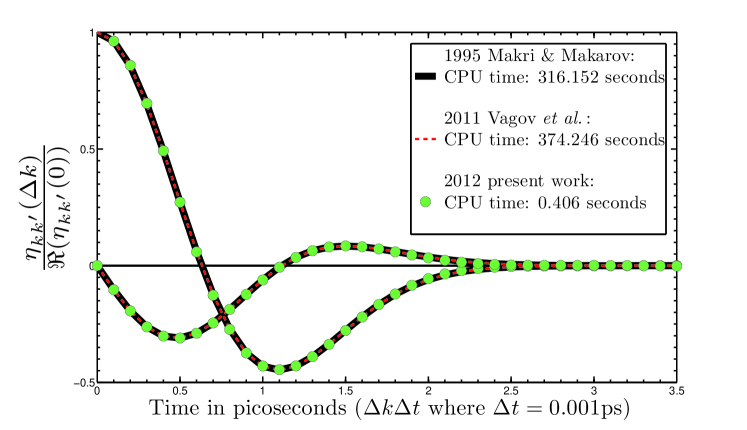
Figure 1: Equations 16, 18 and 20 are equivalent, but equation 20 can be calculated much more efficiently than the other two. Since the values of these curves on the ordinate axis depend on the size of $\Delta t$ (which is a parameter used for numerical computation of the Feynman integral and not a phsyical characteristic of the system), all of these curves are scaled by the real part of the funciton when $\Delta k=0$ in order to have the ordinate axis equal to 1 at most. Here $J(\omega)=0.027{\rm ps^{2}}\omega^{3}e^{(-\nicefrac{{\omega}}{{2.2{\rm ps^{-1}}}})^{2}}$, which is often used to study quantum dots2010Ramsay ; McCutcheon2011a ; Dattani2012 , and $\beta=\frac{1}{k_{B}T}$ with $T=77{\rm K}$. Equation 16 was originally presented in 1995Makri and equation 18 was originally presented in 2011Vagov .

II.3 Strang Splitting

A more sophisticated discretization of the Feynman paths can be made by a Strang splitting, which allows one to calculate the R$\rho$D much more accurately for a given number of time steps in the discretizaton of the Feynman paths. When this splitting is used, the above formulas for $\eta_{kk^{\prime}}$ and $\eta_{kk}$ remain the same for $0<k^{\prime}<k<N$, but different formulas have to be used when either $k$ or $k^{\prime}$, or both, are $0$ or $N$:

$$\eta_{N0} =\int_{N\Delta t-\nicefrac{{\Delta t}}{{2}}}^{N\Delta t}\quad\int_{0}^{\nicefrac{{\Delta t}}{{2}}}\alpha(t^{\prime}-t^{\prime\prime}){\rm d}t^{\prime\prime}{\rm d}t^{\prime}$$ (22)

$$\eta_{00} =\int_{0}^{\nicefrac{{\Delta t}}{{2}}}\int_{0}^{t^{\prime}}\alpha(t^{\prime}-t^{\prime\prime}){\rm d}t^{\prime\prime}{\rm d}t^{\prime}$$ (23)

$$\eta_{NN} =\int_{N\Delta t-\nicefrac{{\Delta t}}{{2}}}^{N\Delta t}\quad\int_{N\Delta t-\nicefrac{{\Delta t}}{{2}}}^{t^{\prime}}\alpha(t^{\prime}-t^{\prime\prime}){\rm d}t^{\prime\prime}{\rm d}t^{\prime}$$ (24)

$$\eta_{k0} =\int_{k\Delta t}^{(k+1)\Delta t}\int_{0}^{\nicefrac{{\Delta t}}{{2}}}\alpha(t^{\prime}-t^{\prime\prime}){\rm d}t^{\prime\prime}{\rm d}t^{\prime}$$ (25)

$$\eta_{Nk} =\int_{N\Delta t-\nicefrac{{\Delta t}}{{2}}}^{N\Delta t}\quad\int_{k\Delta t}^{(k+1)\Delta t}\alpha(t^{\prime}-t^{\prime\prime}){\rm d}t^{\prime\prime}{\rm d}t^{\prime}$$ (26)

Again, most traditionally 1995Makri ; 1995Makri2 ; 1995Makri3 equation 6 is inserted into equations 22 to 26 , which yields (when $J(-\omega)\equiv-J(\omega)$):

$$\eta_{N0} =\frac{2}{\pi}\int_{-\infty}^{\infty}\frac{J(\omega)}{\omega^{2}}\frac{\exp(\nicefrac{{\beta\hbar\omega}}{{2}})}{\sinh(\nicefrac{{\beta\hbar\omega}}{{2}})}\sin^{2}(\nicefrac{{\omega\Delta t}}{{4}})e^{-{\rm i}\omega(t-\nicefrac{{\Delta t}}{{2}})}{\rm d\omega\,\,,}$$ (27)

$$\eta_{00} =\eta_{NN}=\frac{1}{2\pi}\int_{-\infty}^{\infty}\frac{J(\omega)}{\omega^{2}}\frac{\exp(\nicefrac{{\beta\hbar\omega}}{{2}})}{\sinh(\nicefrac{{\beta\hbar\omega}}{{2}})}\left((1-e^{-{\rm i}\omega\nicefrac{{\Delta t}}{{2}}})-{\rm\nicefrac{{i\Delta t\omega}}{{2}}}\right){\rm d}\omega\,\,,\,0<k<N$$ (28)

$$\eta_{k0} =\frac{2}{\pi}\int_{-\infty}^{\infty}\frac{J(\omega)}{\omega^{2}}\frac{\exp(\nicefrac{{\beta\hbar\omega}}{{2}})}{\sinh(\nicefrac{{\beta\hbar\omega}}{{2}})}\sin(\nicefrac{{\omega\Delta t}}{{4}})\sin(\nicefrac{{\omega\Delta t}}{{2}})e^{-{\rm i}\omega(k\Delta t-\nicefrac{{\Delta t}}{{4}})}{\rm d\omega}\,\,,\,0<k<N,$$ (29)

$$\eta_{Nk} =\frac{2}{\pi}\int_{-\infty}^{\infty}\frac{J(\omega)}{\omega^{2}}\frac{\exp(\nicefrac{{\beta\hbar\omega}}{{2}})}{\sinh(\nicefrac{{\beta\hbar\omega}}{{2}})}\sin(\nicefrac{{\omega\Delta t}}{{4}})\sin(\nicefrac{{\omega\Delta t}}{{2}})e^{-{\rm i}\omega(t-k\Delta t-\nicefrac{{\Delta t}}{{4}})}{\rm d\omega}\,\,,\,0<k<N$$ (30)

In the case of $\alpha(t)=\sum_{j}^{K}p_{j}e^{\Omega_{j}t}$ we again find analytical expressions:

$$\eta_{N0} =4\sum_{j=1}^{K}\frac{p_{j}}{\Omega_{j}^{2}}e^{\Omega_{j}(t-\nicefrac{{\Delta t}}{{2}})}\left(\sinh^{2}(\nicefrac{{\Omega_{j}\Delta t}}{{4}})\right)$$ (31)

$$\eta_{00} =\eta_{NN}=2\sum_{j=1}^{M}\frac{p_{j}}{\Omega_{j}^{2}}\left(e^{\nicefrac{{\Omega_{j}\Delta t}}{{4}}}\sinh(\nicefrac{{\Omega_{j}\Delta t}}{{4}})-\nicefrac{{\Delta t\Omega_{j}}}{{4}}\right)$$ (32)

$$\eta_{k0} =4\sum_{j=1}^{K}\frac{p_{j}}{\Omega_{j}^{2}}\sinh(\nicefrac{{\Omega_{j}\Delta t}}{{2}})\sinh\left(\nicefrac{{\Omega_{j}\Delta t}}{{4}}\right)e^{\Omega_{j}(k\Delta t-\nicefrac{{\Delta t}}{{4}})}$$ (33)

$$\eta_{Nk} =4\sum_{j=1}^{K}\frac{p_{j}}{\Omega_{j}^{2}}\sinh(\nicefrac{{\Omega_{j}\Delta t}}{{2}})\sinh\left(\nicefrac{{\Omega_{j}\Delta t}}{{4}}\right)e^{\Omega_{j}(t-k\Delta t-\nicefrac{{\Delta t}}{{4}})}$$ (34)

II.4 Quasi-adiabatic displacement

When the bath is nearly adiabatic, it is helpful to rewrite equation 3 as 1992Makri :

$$H =H_{{\rm OQS}}-H_{{\rm displacement}}+H_{{\rm OQS-bath}}+H_{{\rm bath}}+H_{{\rm displacement}}$$ (35)

$$=H_{{\rm OQS}}-\sum_{\kappa}\frac{c_{\kappa}^{2}s^{2}}{2m_{\kappa}\omega_{\kappa}^{2}}+\sum_{\kappa}c_{\kappa}sQ+\sum_{\kappa}\big{(}\textrm{\textonehalf}m_{\kappa}\dot{Q_{\kappa}}^{2}+\text{\textonehalf}m_{\kappa}\omega_{\kappa}^{2}Q_{\kappa}^{2}\big{)}+\sum_{\kappa}\frac{c_{\kappa}^{2}s^{2}}{2m_{\kappa}\omega_{\kappa}^{2}}$$ (36)

$$\equiv H_{{\rm OQS,displaced}}+\sum_{\kappa}c_{\kappa}sQ+H_{{\rm bath,displaced}}.$$ (37)

$H_{{\rm displacement}}$ is called the “counter term”, and can also be represented in terms of the spectral distribution by recognizing that when the QHOs span a continuous spectrum of frequencies $\omega_{\kappa}$ , we have the relation (remembering equation 4):

$$\sum_{\kappa}\frac{c_{\kappa}^{2}}{2m_{\kappa}\omega_{\kappa}^{2}}=\frac{1}{\pi}\int_{0}^{\infty}\frac{J(\omega)}{\omega}{\rm d}\omega\,.$$ (38)

The influence of $H_{{\rm OQS-bath}}+H_{{\rm bath,displaced}}$ on the R$\rho$D of the displaced OQS is now completely captured by the modified influence phase functional1995Makri ; 1995Makri2 ; 1995Makri3 :

$$\Phi_{{\rm QUAPI}}[s(t),s^{\prime}(t)]=-\int_{0}^{t}\int_{0}^{t^{\prime}}\bigg{(}\left(s(t^{\prime})-s^{\prime}(t^{\prime})\right)\left(\alpha(t^{\prime},t^{\prime\prime})s(t^{\prime\prime})-\alpha^{*}(t^{\prime},t^{\prime\prime})s^{\prime}(t^{\prime\prime})\right)+\frac{{\rm i}}{\hbar\pi}\int_{0}^{t}\int_{0}^{\infty}\frac{J(\omega)}{\omega}{\rm d}\omega\Big{(}s^{+}(t^{\prime})^{2}-s^{-}(t^{\prime})^{2}\Big{)}{\rm\bigg{)}d}t^{\prime\prime}{\rm d}t^{\prime}\,,$$ (39)

where QUAPI stands for Quasi-Adiabatic Propagator Feynman Integral, which is the name for the resulting Feynman integral for the R$\rho$D of the displaced OQS when this new influence phase functional is used. When the bath is nearly adiabatic, the QUAPI is more accurate than a Feynman integral that does not make use of this modified influence phase functional, for a given size of the time step used in the discretizaton of the Feynman paths. The new term in the influence phase functional adds the following term to the $\eta_{kk^{\prime}}$ coefficients when $k=k^{\prime}$:

$$\smash{\raisebox{-2.15277pt}{\begin{tabular}[]{@{}cc@{}}\lx@intercol\hfil*\hfil\lx@intercol\\[-8.61108pt] *&*\end{tabular}}}_{{\rm QUAPI}} =\frac{{\rm i}\Delta t}{\hbar\pi}\int_{0}^{\infty}\frac{J(\omega)}{\omega}{\rm d}\omega$$ (42)

$$\equiv\frac{{\rm i}\Delta t}{\hbar\pi}\lambda\,,$$ (43)

where in the last line we have defined the “bath reorganization energy” by $\lambda$. In equations 16 to 19, and 27 to 30, equation 42 can simply be incorporated into the integrals over $\omega$, but our versions (equations 20, 21, and 31 to 34) are no longer analytic unless an analytic expression exists for $\lambda$. Fortunately an analytic expression exists for $\lambda$ for most forms of $J(\omega)$. Table 1 presents analytic expressions for some of the most popular forms of $J(\omega)$.

II.5 New class of spectral distributions whose bath response functions are analytically expressed as $\alpha(t)=\sum_{j}^{K}p_{j}e^{\Omega_{j}t}$.

This formula is good for testing the spectral distribution corresponding to a bath response function obtained by a least-squares fit, or obtained by a truncation of the (exact) infinite series expression for $\alpha(t)$ table (see table 1 for some examples).

$$J(\omega)=\Re\frac{1}{\pi}(1-e^{-\beta\omega})\sum_{j}^{K}\frac{{\rm i}p_{j}}{\omega-{\rm i}\Omega_{j}}$$ (44)

III Conclusions

We have presented general formulas for the $\eta$ coefficients in the discretized influence functional of the Feynman-Vernon model, in terms of the bath response function. These formulas can then be used to derive the form of the $\eta$ coefficients presented by Makarov and Makri in 19951995Makri ; 1995Makri2 , and the form presented by Vagov et al. in 20112011Vagov , both which involve improper integrals of the spectral distribution and have at least one infinite integration bound. However, when the bath response function can be expressed analytically (which is almost always the case, as shown in table 1), our general formulas for the $\eta$ coefficients can almost always be derived analytically too. Figure 1 shows that the evaluation of these analytic formulas can be more than 900 times faster than obtaining the exact same results by numerically integrating forms for the $\eta$ coefficients in the traditional ways.

If there is a case where the bath response function can be expressed analytically, but the integrals in equation 14, 15 and/or 22 to 26 cannot be evaluated analytically (we do not know of such a case, but cannot rule out the possibility that it exists), we recommend to numerically integrate these equations, rather than to numerically integrate the more traditional forms presented in equations 16 to 19 and 27 to 30. This is because these integrals have finite bounds, which are very small (about the size of the time steps in the discretization of the Feynman paths), while the more traditional forms involve numerically integrating the spectral distribution over infinite bounds.

When the bath response function cannot be expressed analytically, it may still be more convenient to obtain it by numerically integrating equation 5, 6 or 7, and then to fit it to a sum of complex-weighted complex exponentials. This is because Feynman integrals for calculating the reduced density operator dynamics in open quantum systems are usually used for benchmarking other techniques, and many popular techniques require this form for the bath response function, and when benchmarking it is always best to keep as many parameters of the model consistent across all methods being benchmarked. When fitting a bath response function to this form, equation 44 is useful for testing the quality of the fit in terms of how well the fitted bath response function corresponds to the original desired spectral distribution. This formula is equally useful in cases when the bath response function is naturally represented in the form of equation 1 (as in the examples in table 1), since it can give an indication of how many terms in the infinite series are required in order to be sure that one is using a bath response function which corresponds to a spectral distribution similar enough to the original desired one.

IV Special Cases (Appendix)

The results in equations 20, 21 and 31 to 34 can readily be applied for many of the spectral distributions listed in table 1, by substituting the appropriate values of $p_{j}$ and $\Omega_{j}$.

One of the most popular spectral distribution forms is currently the Lorentz-Drude/Debye (LDD) form which has been used extensively in experimental determinations of spectral distributions 2006Zigmantas ; 2007Read ; 2008Read , and in various OQS studies (2009Ishizaki and various other studies of this same system that compare to this result, including ones involving DIFs for Feynman integrals 2011Nalbach ; Nalbach2011 ):

$$J(\omega)=\frac{\omega}{\pi}\frac{\lambda\gamma}{\gamma^{2}+\omega^{2}}.$$ (45)

The first spectral distribution form presented in table 1 is a generalization of this LDD form, which allows for multiple peaks to be included at various locations defined by $\{\tilde{\omega}_{j}\}$. In the case where only one term in the sum exists, and $\tilde{\omega}=0$, equation 45 is recovered. The bath response function for equation 45 can be obtained analytically in the form of equation 1 by a simple application of residue calculus, leading to the well-known Matsubara series. Since the Matsubara series converges extremely slowly, we have presented a series based on the very recent [N-1/N] Padé decomposition technique in Hu2010 (a more clever application of residue calculus), which is also of the form in equation 1, but converges with much fewer terms. The label [N-1/N] denotes that the Padé approximant is a rational funciton where the numerator is a polynomial of degree N-1, and the denominator is a polynomial of degree N. N effectively becomes the number of exponential terms in $\alpha(t)$ that specifically arise due to this technique for expressing $\alpha(t)$ in the form of equation 1 (more details about this technique can be found in Hu2010 ; Hu2011 ). This representation of $\alpha(t)$ becomes more and more accurate as $N$ is increased. The Padé parameters $\{\xi_{n}$,$\Xi_{n}\}$ are given in table 2. The total number of terms in $\alpha(t)$ is given by $K=2J+N$, where $J$ is the number lorentzian terms of each type in $J(\omega)$.

The second spectral distribution form presented in the table below is used in studies where the $J(\omega)$ for a system is predicted using a molecular dynamics simulationDamjanovic2002 ; Olbrich2011a . It is the same as the first spectral distribution form in table 1, but with the prefactor $\omega$ replaced by $\tanh(\frac{\beta\omega}{2})$ in an attempt to remove the temperature dependence of $J(\omega)$ which is inherent due to the nature of the molecular dynamics technique that is used to calculate it. As for the first $J(\omega)$ presented, the bath response function for this $J(\omega)$ was put into the form of equation 1 by the Padé decomposition, except that in this case only the imaginary component requires a Padé decomposition treatment. The total number of terms in $\alpha(t)$ is again given by $K=2J+N$.

The third spectral distribution form presented is known as the Meier-Tanor decomposition and has been widely used since its introduction in 1999Meier1999 . It is similar to forms used for the spectral distribution function in Shugard1978 and Thorwart2004 . Here we do not use a Padé decomposition treatment, but rather present the same representation of $\alpha(t)$ in the form of equation 1 as was originally presented by Meier and Tanor (using a Matsubara-style decomposition) in Meier1999 . The total number of terms in $\alpha(t)$ is again given by $K=2J+N$, where $N$ now denotes the number of terms contributed by the Matsubara-style decomposition. Once again, this representation of $\alpha(t)$ beocmes more and more accurate as $N$ is increased.

Finally, formulas 14, 15 and 22 to 26 can readily be applied to other spectral distribution functions when an analytic expression for $\alpha(t)$ exists. One very popular class of spectral distribution functions for which $\alpha(t)$ can be calculated analytically (resulting in a form different from equation 1) is the class of functions of the form $J(\omega)\propto\omega^{s}e^{-(\nicefrac{{\omega}}{{\omega_{c}}})^{q}}.$ An analytic form for $\alpha(t)$ and the reorganization energy $\lambda$ for this class of spectral distribution functions is presented in table 1 below. The result of evaluating this formula is compared to the $\alpha(t)$ obtained by numerical integration with essentially exact agreement, and this comparison is presented in the supplementary material.

Table 1: Analytic formulas for the bath response functions $\alpha(t)$ and reorganization energies $\lambda$ of various selected spectral distribution functions. For the first three cases, $K=2J+N$, where $N$ is the number of terms in $\alpha(t)$ arising from the Padé (for the first two forms of $J(\omega)$) or Matsubara-style (for the third form of $J(\omega)$) decomposition. All formulas presented here can be computed easily for any value of $K$ in our open source MATLAB program that supplements this paper. $\psi_{s}(\cdot)$ is the polygamma function, which is a built-in function that is evaluated quickly in MATLAB, Mathematica, and most computing software.

$J(\omega)=\frac{\omega}{\pi}\sum_{j}^{J}\bigg{(}\frac{\lambda{}_{j}\gamma_{j}}{\gamma_{j}^{2}+(\omega-\tilde{\omega}_{j})^{2}}+\frac{\lambda{}_{j}\gamma_{j}}{\gamma_{j}^{2}+(\omega+\tilde{\omega}_{j})^{2}}\bigg{)}$	$\alpha(t)=\sum_{j}^{K}p_{j}e^{\Omega_{j}t}$
$\quad\quad p_{j=}\begin{cases}\frac{\lambda{}_{j}}{\beta}\left(1-\sum_{n=1}^{N}\frac{2\Xi_{n}\Omega_{j}^{2}}{\nu_{n}^{2}-\Omega_{j}^{2}}\right)+{\rm i}\frac{\lambda{}_{j}\Omega_{j}}{2}\,,&j\in[0,J]\\ \frac{\lambda{}_{j}}{\beta}\left(1-\sum_{n=1}^{N}\frac{2\Xi_{n}\Omega_{j}^{2}}{\nu_{n}^{2}-\Omega_{j}^{2}}\right)+{\rm i}\frac{\lambda{}_{j}\Omega_{j}}{2}\,,&j\in[J+1,2J]\\ -\sum_{m=1}^{J}\frac{4\lambda_{m}\gamma_{m}}{\beta}\frac{\Xi_{j}\nu_{j}\big{(}|\Omega_{m}|^{2}-\nu_{j}^{2}\big{)}}{\lvert\nu_{j}^{2}-\Omega_{m}^{2}\rvert^{2}}\,,&j\in[2J+1,K]\end{cases}$
$\hskip 8.00002pt\hskip 8.00002pt\Omega_{j}=\begin{cases}-\gamma{}_{j}+{\rm i}\tilde{\omega}_{j}\,,&j\in[0,J]\\ -\gamma{}_{j}-{\rm i}\tilde{\omega}_{j}\,,&j\in[J+1,2J]\\ -\nu_{j}\,,&j\in[2J+1,K]\end{cases}$		${\color[rgb]{1,1,1}\begin{cases}{\color[rgb]{0,0,0}}\\ {\color[rgb]{0,0,0}(\cdot)_{J+j}}&{\color[rgb]{0,0,0}{\color[rgb]{0,0,0}=(\cdot)_{j}}}\\ {\normalcolor\nu_{n}}&{\normalcolor=\frac{2\pi\xi_{n}}{\beta}}\end{cases}}$
$\hskip 8.00002pt\hskip 8.00002pt\lambda=\sum_{j}^{J}\lambda_{j}$	$\{\xi_{n},\Xi_{n}\}$ are the [N-1/N] Padé parameters for the Bose-Einstein distribution (see table 2)
$J(\omega)=\frac{1}{\pi}\tanh\big{(}\frac{\beta\omega}{2}\big{)}\sum_{j}^{J}\bigg{(}\frac{\lambda_{j}\gamma_{j}}{\gamma_{j}^{2}+(\omega-\tilde{\omega}_{j})^{2}}+\frac{\lambda_{j}\gamma_{j}}{\gamma_{j}^{2}+(\omega+\tilde{\omega}_{j})^{2}}\bigg{)}$	$\alpha(t)=\sum_{j}^{K}p_{j}e^{\Omega_{j}t}$	$J(\omega)$ introduced by Damjanovic et al. Damjanovic2002 ; Gutierrez2010
$\hskip 8.00002pt\hskip 8.00002ptp_{j}=\begin{cases}\frac{\lambda_{j}}{2}+{\rm i}\frac{2\lambda_{j}}{\beta}\sum_{n=1}^{N}\frac{\Xi_{n}\Omega_{j}}{\nu_{n}^{2}-\Omega_{j}^{2}}\,,&j\in[0,J]\\ \frac{\lambda_{j}}{2}+{\rm i}\frac{2\lambda_{j}}{\beta}\sum_{n=1}^{N}\frac{\Xi_{n}\Omega_{j}}{\nu_{n}^{2}-\Omega_{j}^{2}}\,,&j\in[J+1,2J]\\ -{\rm i}\frac{4\Xi_{j}}{\beta}\sum_{m=1}^{J}\frac{\tilde{\gamma}_{m}\tilde{\lambda}_{m}\big{(}|\Omega_{m}|^{2}-\nu_{j}^{2}\big{)}}{\lvert\nu_{j}^{2}-\Omega_{m}^{2}\rvert^{2}}\,,&j\in[2J+1,K]\end{cases}$
$\hskip 8.00002pt\hskip 8.00002pt\Omega_{j}=\begin{cases}-\gamma_{j}+{\rm i}\tilde{\omega}_{j}\,,&j\in[0,J]\\ -\gamma_{j}-{\rm i}\tilde{\omega}_{j}\,,&j\in[J+1,2J]\\ -\nu_{j}\,,&j\in[2J+1,K]\end{cases}$		${\color[rgb]{1,1,1}\begin{cases}{\color[rgb]{0,0,0}}\\ {\color[rgb]{0,0,0}(\cdot)_{J+j}}&{\color[rgb]{0,0,0}{\color[rgb]{0,0,0}=(\cdot)_{j}}}\\ {\normalcolor\nu_{n}}&{\normalcolor=\frac{2\pi\xi_{n}}{\beta}}\end{cases}}$
	$\{\xi_{n},\Xi_{n}\}=$are the [N-1/N] Padé parameters for the Fermi-Dirac distribution (see table 2)
$J(\omega)=\frac{\pi\omega}{2}\sum_{j}^{K}\frac{\lambda_{j}}{\big{(}\gamma_{j}^{2}+(\omega+\tilde{\omega}_{j})^{2}\big{)}\big{(}\gamma_{j}^{2}+(\omega-\tilde{\omega}_{j})^{2}\big{)}}$	$\alpha(t)=\sum_{j}^{K}p_{j}e^{\Omega_{j}t}$	Meier-Tanor decomposition Meier1999
$\quad\quad p_{j=}\begin{cases}\frac{\lambda j}{\tilde{\omega}_{j}\gamma_{j}}\bigg{(}\coth\big{(}\frac{\beta}{2}(\tilde{\omega}_{j}+{\rm i}\gamma_{j})\big{)}+{\rm i}\bigg{)}\,,&j\in[0,J]\\ \frac{\lambda_{j}}{\tilde{\omega}_{j}\gamma_{j}}\bigg{(}\coth\big{(}\frac{\beta}{2}(\tilde{\omega}_{j}-{\rm i}\gamma_{j})\big{)}-{\rm i}\bigg{)}\,,&j\in[J+1,2J]\\ -\frac{\pi}{\beta}\sum_{n=1}^{N}\frac{\nu_{j}\lambda_{n}}{\big{(}\gamma_{n}^{2}+(i\nu_{j}+\tilde{\omega}_{n})^{2}\big{)}\big{(}\gamma_{n}^{2}+(i\nu_{j}-\tilde{\omega}_{n})^{2}\big{)}}\,,&j\in[2J+1,K]\end{cases}$
$\hskip 8.00002pt\hskip 8.00002pt\Omega_{j}=\begin{cases}-\gamma_{j}+{\rm i}\tilde{\omega}_{j}\,,&j\in[0,J]\\ -\gamma_{j}-{\rm i}\tilde{\omega}_{j}\,,&j\in[J+1,2J]\\ -\nu_{j}\,,&j\in[2J+1,K]\end{cases}$		${\color[rgb]{1,1,1}\begin{cases}{\color[rgb]{0,0,0}}\\ {\color[rgb]{0,0,0}(\cdot)_{J+j}}&{\color[rgb]{0,0,0}{\color[rgb]{0,0,0}=(\cdot)_{j}}}\\ {\normalcolor\nu_{n}}&{\normalcolor=\frac{2\pi n}{\beta}}\end{cases}}$
$\hskip 8.00002pt\hskip 8.00002pt\lambda=\frac{\pi^{2}}{8\gamma(\gamma^{2}+\omega_{0}^{2})}\sum_{j}^{K}\lambda_{j}$
$J(\omega)=A\omega^{s}e^{-\nicefrac{{\omega}}{{\omega_{c}}}}$	$\alpha(t)=-s!\omega_{c}^{s+1}\left(z+(-1)^{s+1}z^{*}\right)$	See Leggett1987 for a detailed use of this $J(\omega)$
$z\equiv\big{(}\frac{1}{(\omega_{c}t+i)^{s+1}}\big{)}-\frac{2\Re\big{(}\psi_{s}(\frac{1+i\omega_{c}t}{\beta\omega_{c}})\big{)}}{s!(\beta\omega_{c})^{s+1}}-i\frac{\sin\big{(}(s+1)\arctan(\omega_{c}t)\big{)}}{(1+\omega_{c}^{2}t^{2})^{(s+1)/2}}$
$\hskip 8.00002pt\hskip 8.00002pt\lambda=A\omega_{c}^{s}\Gamma(s)$
$J(\omega)=A\omega^{s}e^{-(\nicefrac{{\omega}}{{\omega_{c}}})^{q}}\,s>0\,,\,\omega_{c}>0\,,\,q>0$
$\hskip 8.00002pt\hskip 8.00002pt\lambda=\frac{A}{q}\omega_{c}^{s}\Gamma(\frac{s}{q})$

Table 2: [N-1/N] Padé parameters for the Bose-Einstein and Fermi-Dirac distribution functions (first presented in Hu2010 and in more detail in Hu2011 ). $\{\Xi_{n},\xi_{n}\}$ can be calculated easily for all $n$, for arbitrary values of $N$ in our open source MATLAB program that supplements this paper. The matrix $\Lambda$ is a 2N$\times$2N, and $\tilde{\Lambda}$ is a 2N-1$\times$2N-1. The indices $n$ run from 1 to half the number of non-zero eigenvalues of the corresponding matrix. The number of non-zero eigenvalues will always be even, because the eigenvalues of these particular matrices come in pairs, for example ($\xi_{n},-\xi_{n}$); and for matrices with an odd number of eigenvalues, the unpaired eigenvalue will always be 0.

$\{\pm\xi_{n}\}=\text{eigenvalues}(\Lambda^{-1})$	$\{\pm\zeta_{n}\}=\text{eigenvalues}(\tilde{\Lambda}^{-1})$
Bose-Einstein	Fermi-Dirac
$\Lambda_{cd}=\frac{\delta_{c,d\pm 1}}{2\sqrt{(2c+1)(2d+1)}}$	$\Lambda_{cd}=\frac{\delta_{c,d\pm 1}}{2\sqrt{(2c-1)(2d-1)}}$
$\tilde{\Lambda}_{cd}=\frac{\delta_{c,d\pm 1}}{2\sqrt{(2c+3)(2d+3)}}$	$\tilde{\Lambda}_{cd}=\frac{\delta_{c,d\pm 1}}{2\sqrt{(2c+1)(2d+1)}}$
$\Xi_{n}=(N^{2}+\frac{3}{2}N)\frac{\prod_{m=1}^{N-1}(\zeta_{m}^{2}-\xi_{n}^{2})}{\prod_{m\neq n}^{N}(\xi_{m}^{2}-\xi_{n}^{2})}$	$\Xi_{n}=(N^{2}+\frac{1}{2}N)\frac{\prod_{m=1}^{N-1}(\zeta_{m}^{2}-\xi_{n}^{2})}{\prod_{m\neq n}^{N}(\xi_{m}^{2}-\xi_{n}^{2})}$

V Acknowledgements

We would like to thank Thomas E. Markland whose MSc. thesis inspired this work. For valuable comments on the manuscript, and for the derivation of equation 44, credit is due to David E. Manolopoulos. N.S.D. thanks the Clarendon Fund and the NSERC/CRSNG of/du Canada for financial support. F.A.P. thanks the Leverhulme Trust for financial support. We dedicate this manuscript to Albert Einstein and Brendon W. Lovett, who were both born on this day.

References

- [1] Ana Damjanović, Ioan Kosztin, Ulrich Kleinekathöfer, and Klaus Schulten. Excitons in a photosynthetic light-harvesting system: A combined molecular dynamics, quantum chemistry, and polaron model study. Physical Review E, 65(3), March 2002.
- [2] Nikesh S. Dattani. Numerical Feynman integrals with physically inspired interpolation: Faster convergence and significant reduction of computational cost. AIP Advances, 2(1):012121, 2012.
- [3] Richard Phillips Feynman, Albert R Hibbs, and Daniel F Styer. Quantum Mechanics and Path Integrals. Dover Publications Inc., emended edition, 2010.
- [4] Richard Phillips Feynman and F L Vernon Jr. The Theory of a General Quantum System Interacting with a Linear Dissipative System. Annals of Physics, 24:118–173, 1963.
- [5] R Gutiérrez, R Caetano, P B Woiczikowski, T Kubar, M Elstner, and G Cuniberti. Structural fluctuations and quantum transport through DNA molecular wires: a combined molecular dynamics and model Hamiltonian approach. New Journal of Physics, 12(2):023022, February 2010.
- [6] Jie Hu, Meng Luo, Feng Jiang, Rui-Xue Xu, and Yijing Yan. Padé spectrum decompositions of quantum distribution functions and optimal hierarchical equations of motion construction for quantum open systems. The Journal of chemical physics, 134(24):244106, June 2011.
- [7] Jie Hu, Rui-Xue Xu, and Yijing Yan. Communication: Padé spectrum decomposition of Fermi function and Bose function. The Journal of chemical physics, 133(10):101106, September 2010.
- [8] Akihito Ishizaki and Graham R Felming. Theoretical examination of quantum coherence in a photosynthetic system at physiological temperature. Proceedings of the National Academy of Sciences, 106(41):17255–17260, 2009.
- [9] O. Kühn. Laser control of intramolecular hydrogen transfer reactions: A real-time path integral approach. The European Physical Journal D - Atomic, Molecular and Optical Physics, 6(1):49–55, March 1999.
- [10] A. Leggett, S. Chakravarty, A. Dorsey, Matthew Fisher, Anupam Garg, and W. Zwerger. Dynamics of the dissipative two-state system. Reviews of Modern Physics, 59(1):1–85, January 1987.
- [11] N MAKRI. IMPROVED FEYNMAN PROPAGATORS ON A GRID AND NONADIABATIC CORRECTIONS WITHIN THE PATH INTEGRAL FRAMEWORK. CHEMICAL PHYSICS LETTERS, 193(5):435–445, June 1992.
- [12] N MAKRI. NUMERICAL PATH-INTEGRAL TECHNIQUES FOR LONG-TIME DYNAMICS OF QUANTUM DISSIPATIVE SYSTEMS. JOURNAL OF MATHEMATICAL PHYSICS, 36(5):2430–2457, May 1995.
- [13] N Makri, E J Sim, D E Makarov, and M Topaler. Long-time quantum simulation of the primary charge separation in bacterial photosynthesis. PROCEEDINGS OF THE NATIONAL ACADEMY OF SCIENCES OF THE UNITED STATES OF AMERICA, 93(9):3926–3931, April 1996.
- [14] Nancy Makri and Dmitrii E Makarov. Tensor propagator for iterative quantum time evolution of reduced density matrices. I. Theory. Journal of Chemical Physics, 102(11):4600–4610, 1995.
- [15] Nancy Makri and Dmitrii E Makarov. Tensor propagator for iterative quantum time evolution of reduced density matrices. II. Numerical methodology. Journal of Chemical Physics, 102(11):4611–4618, 1995.
- [16] DPS McCutcheon, NS Dattani, EM Gauger, BW Lovett, and A Nazir. A general approach to quantum dynamics using a variational master equation: Application to phonon-damped Rabi rotations in quantum dots. Physical Review B, 84(1):2–5, 2011.
- [17] Christoph Meier and David J. Tannor. Non-Markovian evolution of the density operator in the presence of strong laser fields. The Journal of Chemical Physics, 111(8):3365, August 1999.
- [18] Sadao Nakajima. On Quantum Theory of Transport Phenomena. Progress of Theoretical Physics, 20(6):948–959, 1958.
- [19] P. Nalbach, D. Braun, and M. Thorwart. Exciton transfer dynamics and quantumness of energy transfer in the Fenna-Matthews-Olson complex. Physical Review E, 84(4), October 2011.
- [20] Peter Nalbach, Akihito Ishizaki, Graham R Fleming, and Michael Thorwart. Iterative path-integral algorithm versus cumulant time-nonlocal master equation approach for dissipative biomolecular exciton transport. NEW JOURNAL OF PHYSICS, 13, June 2011.
- [21] Carsten Olbrich, Thomas L C Jansen, Jörg Liebers, Mortaza Aghtar, Johan Strümpfer, Klaus Schulten, Jasper Knoester, and Ulrich Kleinekathöfer. From atomistic modeling to excitation transfer and two-dimensional spectra of the FMO light-harvesting complex. The journal of physical chemistry. B, 115(26):8609–21, July 2011.
- [22] A. Ramsay, T. Godden, S. Boyle, E. Gauger, A. Nazir, B. Lovett, A. Fox, and M. Skolnick. Phonon-Induced Rabi-Frequency Renormalization of Optically Driven Single InGaAs/GaAs Quantum Dots. Physical Review Letters, 105(17), October 2010.
- [23] A J Ramsay, Achanta Venu Gopal, E M Gauger, A Nazir, B W Lovett, A M Fox, and M S Skolnick. Damping of Exciton Rabi Rotations by Acoustic Phonons in Optically Excited In GaAs/GaAs Quantum Dots. Phys. Rev. Lett., 104(1):17402, January 2010.
- [24] Elizabeth L Read, Gregory S Engel, Tessa R Calhoun, Tomas Mancal, Tae Kyu Ahn, Robert E Blankenship, and Graham R Fleming. Cross-peak-specific two-dimensional electronic spectroscopy. PROCEEDINGS OF THE NATIONAL ACADEMY OF SCIENCES OF THE UNITED STATES OF AMERICA, 104(36):14203–14208, September 2007.
- [25] Elizabeth L Read, Gabriela S Schlau-Cohen, Gregory S Engel, Jianzhong Wen, Robert E Blankenship, and Graham R Fleming. Visualization of excitonic structure in the Fenna-Matthews-Olson photosynthetic complex by polarization-dependent two-dimensional electronic spectroscopy. BIOPHYSICAL JOURNAL, 95(2):847–856, July 2008.
- [26] Gerhard Ritschel, Jan Roden, Walter T Strunz, and Alexander Eisfeld. An efficient method to calculate excitation energy transfer in light-harvesting systems: application to the Fenna-Matthews-Olson complex. New Journal of Physics, 13(11):113034, November 2011.
- [27] Mary Shugard, John C. Tully, and Abraham Nitzan. Stochastic classical trajectory approach to relaxation phenomena. I. Vibrational relaxation of impurity molecules in solid matrices. The Journal of Chemical Physics, 69(1):336, July 1978.
- [28] Y TANIMURA and R KUBO. TIME EVOLUTION OF A QUANTUM SYSTEM IN CONTACT WITH A NEARLY GAUSSIAN-MARKOFFIAN NOISE BATH. JOURNAL OF THE PHYSICAL SOCIETY OF JAPAN, 58(1):101–114, January 1989.
- [29] Yoshitaka Tanimura. Nonperturbative expansion method for a quantum system coupled to a harmonic-oscillator bath. Phys. Rev. A, 41(12):6676–6687, June 1990.
- [30] M. Thorwart and P. Jung. Dynamical Hysteresis in Bistable Quantum Systems. Physical Review Letters, 78(13):2503–2506, March 1997.
- [31] M Thorwart, E Paladino, and M Grifoni. Dynamics of the spin-boson model with a structured environment. Chemical Physics, 296(2-3):333–344, January 2004.
- [32] A Vagov, M D Croitoru, M Glässl, V M Axt, and T Kuhn. Real-time path integrals for quantum dots: Quantum dissipative dynamics with superohmic environment coupling. Phys. Rev. B, 83(9):94303, March 2011.
- [33] Willard H Wells. Quantum Formalism Adapted to Radiation in a Coherent Field. Annals of Physics, 12:1–40, 1961.
- [34] Donatas Zigmantas, Elizabeth L Read, Tomas Mancal, Tobias Brixner, Alastair T Gardiner, Richard J Cogdell, and Graham R Fleming. Two-dimensional electronic spectroscopy of the B800-B820 light-harvesting complex. PROCEEDINGS OF THE NATIONAL ACADEMY OF SCIENCES OF THE UNITED STATES OF AMERICA, 103(34):12672–12677, August 2006.
- [35] Robert Zwanzig. Ensemble method in the theory of irreversibility. The Journal of Chemical Physics, 33(5):1338–1341, 1960.