Abstract

Henri Poincaré formulated the mathematics of the Lorentz transformations, known as the Poincaré group. He also formulated the Poincaré sphere for polarization optics. It is shown that these two mathematical instruments can be combined into one mathematical device which can address the internal space-time symmetries of elementary particles, decoherence problems in polarization optics, entropy problems, and Feynman’s rest of the universe.

Presented at the Fedorov Memorial Symposium: International Conference ”Spins and Photonic Beams at Interface,” dedicated to the 100th anniversary of F.I.Fedorov (1911-1994) (Minsk, Belarus, 2011)

1 Introduction

It was Henri Poincarś who worked out the mathematics of Lorentz transformations before Einstein and Minkowski. Poincaré’s interest in mathematics covers many other areas of physics.

Among them, his Poincaré sphere serves as geometrical representation of the Stokes parameters. While there are four Stokes parameters, the traditional Poincaré sphere is based on only three of those parameters [1, 2, 3].

In this report, we show that the concept of the Poincaré sphere can be extended to accommodate all four Stokes parameters, and show that this extended Poincaré sphere can be used as a representation of the Lorentz group applicable to the four-component Minkowski space. In this way, it is possible to use the Poincarś sphere as a picture of the internal space-time symmetries as defined by Wigner in 1939 [4].

Throughout the paper, we shall use the two-by-two matrix formulation of the Lorentz group [5, 6]. The basic advantage is that this representation is the natural language for the two-by-two representation of the four Stokes parameters. Indeed, this two-by-two representation speaks one language applicable to two different branches of physics, as is illustrated in Fig. 1.

Let us consider a particle moving along a given direction. We can rotate the system around this direction, and boost along this direction. We can also rotate around and boost along two orthogonal directions perpendicular to the direction of the momentum. These operations can be written in the form of two-by-two matrices. In this way, we can construct a two-by-two representation of the Lorentz group.

In this report, we use the same set of two-by-two matrices to perform transformations on the Stokes parameters and the Poincaré sphere. While the original three-dimensional Poincaré sphere is based only on three of the four Stokes parameters, it is possible to extend its geometry to accommodate all four parameters. With these parameters, we can address the degree of polarization between the two orthogonal components of electric field perpendicular to the momentum. In order to deal with this problem, we introduce the decoherence parameter derivable from the traditional degree of polarization. Since this parameter is greater than zero and smaller than one, we can write it as $\sin\chi$, and define $\chi$ as the decoherence angle.

One remarkable aspect of this decoherence parameter is that it is invariant under Lorentz transformations. If the symmetry of the Poincaré sphere is translated into the space-time symmetry, the decoherence parameter remains Lorentz-invariant like the particle mass in the space-time symmetry.

Furthermore, to every $\sin\chi$, there is $\cos\chi$, and their symmetry is well known. Thus we can consider another Poincaré sphere with the same decoherence angle. The second Poincaré sphere could serve as another illustrative example of Feynman’s rest of the universe [7, 8].

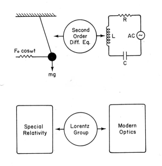
Figure 1: One mathematical instrument for two different branches of physics. As one second-order differential equation takes care of the resonances in the oscillator system and also in the $LCR$ circuit, the Lorentz group can serve as the basic mathematical language for special relativity and modern optics.

In Sec. 2, it was noted that Poincaré was the first one to formulate group of Lorentz transformations for the space-time variables. This transformation law can be translated into the language of Naimark’s two-by-two Naimark representation. Einstein later derived his $E=mc^{2}$ by advancing the concept of the energy-momentum four-vector obeying the same transformation law as that of the space-time coordinates. Thus, the two-by-two representation is possible also for the momentum-energy four-vector.

When Einstein was formulating his special relativity, he did not consider internal space-time structures or symmetries of the particles. Also in Sec. 2, it is shown possible to study Wigner’s little groups using the two-by-two representation. Wigner’s little groups dictate the internal space-time symmetries of elementary particles. They are the subgroups of the Lorentz group whose transformations leave the four-momentum of the given particle invariant [4, 9].

In Sec. 3, we first note that the same two-by-two matrices are applicable to two-component Jones vectors. However, the Jones vector cannot address the problem of coherence between two transverse components of the optical beam. This is why the four-component Stokes parameters are needed. The same Lorentz group can be used for the four-component Stokes parameters, and Stokes parameters are like four-vectors, as in the case of energy-momentum four vectors. It is noted however, the degree of coherence remains invariant under Lorentz transformations.

In Sec. 4, we use the geometry of the Poincaré sphere to describe the Stokes parameters and their transformation properties. It is shown that three different radii are needed to describe them fully. The traditional radius lies between the maximum and minimum radii. It is shown that $\left(S_{0}^{2}-R^{2}\right)$ remains lorentz-invariant, where $S_{0}$ and $R$ are the maximum radius and the traditional radius respectively. This Lorentz-invariant quantity is dictated by the decoherence parameter. The entropy question is also discussed, and this entropy is shown to be Lorentz-invariant.

In Sec. 5, it is shown possible to define another Poincaré sphere in order to deal with variations of the decoherence parameter and the entropy. It is shown that this second Poincaré sphere can serve as another example of Feynman’s rest of the universe [7].

In the the Appendix, we shoe how the two-by-two transformation matrix can be translated into the four-by-four matrix applicable to the Missourian four-vector.

2 Poincaré Group, Einstein, and Wigner

The Lorentz group starts with a group of four-by-four matrices performing Lorentz transformations on the Minkowskian vector space of $(t,z,x,y),$ leaving the quantity

$$t^{2}-z^{2}-x^{2}-y^{2}$$ (1)

invariant. It is possible to perform this transformation using two-by-two representations [5]. This mathematical aspect is known as the $SL(2,c)$ as the universal covering group for the Lorentz group.

In this two-by-two representation, we write the four-vector as a matrix

$$X=\pmatrix{t+z&x-iy\cr x+iy&t-z}.$$ (2)

Then its determinant is precisely the quantity given in Eq.(1). Thus the Lorentz transformation on this matrix is a determinant-preserving transformation. Let us consider the transformation matrix as

$$G=\pmatrix{\alpha&\beta\cr\gamma&\delta},\qquad G^{\dagger}=\pmatrix{\alpha^{*}&\gamma^{*}\cr\beta^{*}&\delta^{*}},$$ (3)

with

$$\det{(G)}=1.$$ (4)

This matrix has six independent parameters. The group of these $G$ matrices is known to be locally isomorphic to the group of four-by-four matrices performing Lorentz transformations on the four-vector $(t,z,x,y)$. In other word, for each $G$ matrix there is a corresponding four-by-four Lorentz-transform matrix, as is illustrated in the Appendix.

The matrix $G$ is not a unitary matrix, because its Hermitian conjugate is not always its inverse. The group can have a unitary subgroup called $SU(2)$ performing rotations on electron spins. As far as we can see, this $G$-matrix formalism was first presented by Naimark in 1954 [5]. Thus, we call this formalism the Naimark representation of the Lorentz group. We shall see first that this representation is convenient for studying space-time symmetries of particles. We shall then note that this Naimark representation is the natural language for the Stokes parameters in polarization optics.

With this point in mind, we can now consider the transformation

$$X^{\prime}=GXG^{\dagger}$$ (5)

Since $G$ is not a unitary matrix, it is not a unitary transformation. In order to tell this difference, we call this “Naimark transformation.” This expression can be written explicitly as

$$\pmatrix{t^{\prime}+z^{\prime}&x^{\prime}-iy^{\prime}\cr x+iy&t^{\prime}-z^{\prime}}=\pmatrix{\alpha&\beta\cr\gamma&\delta}\pmatrix{t+z&x-iy\cr x+iy&t-z}\pmatrix{\alpha^{*}&\gamma^{*}\cr\beta^{*}&\delta^{*}},$$ (6)

For this transformation, we have to deal with four complex numbers. However, for all practical purposes, we may work with two Hermitian matrices

$$Z(\delta)=\pmatrix{e^{i\delta/2}&0\cr 0&e^{-i\delta/2}},\qquad R(\delta)=\pmatrix{\cos(\theta/2)&-\sin(\theta/2)\cr\sin(\theta/2)&\cos(\theta/2)},$$ (7)

and two symmetric matrices

$$B(\mu)=\pmatrix{e^{\mu/2}&0\cr 0&e^{-\mu/2}},\qquad S(\lambda)=\pmatrix{\cosh(\lambda/2)&\sinh(\lambda/2)\cr\sinh(\lambda/2)&\cosh(\lambda/2)}$$ (8)

The two Hermitian matrices in Eq.(7) lead to rotations around the $z$ and $y$ axes respectively. The symmetric matrices in Eq.(8) perform Lorentz boosts along the $z$ and $x$ directions.

Repeated applications of these four matrices will lead to the most general form the of the most general form of the $G$ matrix of Eq.(3) with six independent parameters. For each two-by-two Naimark transformation, there is a four-by-four matrix performing the corresponding Lorentz transformation on the four-component four vector. In the appendix, the four-by-four equivalents are given for the matrices of Eq.(7) and Eq.(8).

It was Einstein who defined the energy-momentum four vector, and showed that it also has the same Lorentz-transformation law as the space-time four-vector. We write the energy-momentum four vector as

$$P=\pmatrix{E+p_{z}&p_{x}-ip_{y}\cr p_{x}+ip_{y}&E-p_{z}},$$ (9)

with

$$\det{(P)}=E^{2}-p_{x}^{2}-p_{y}^{2}-p_{z}^{2},$$ (10)

which means

$$\det{{p}}=m^{2},$$ (11)

where $m$ is the particle mass.

Now Einstein’s transformation law can be written as

$$P^{\prime}=GMG^{\dagger},$$ (12)

or explicitly

$$\pmatrix{E^{\prime}+p_{z}^{\prime}&p_{x}^{\prime}-ip_{y}^{\prime}\cr p^{\prime}_{x}+ip^{\prime}_{y}&E^{\prime}-p^{\prime}_{z}}=\pmatrix{\alpha&\beta\cr\gamma&\delta}\pmatrix{E+p_{z}&p_{x}-ip_{y}\cr p_{x}+ip_{y}&E-p_{z}}\pmatrix{\alpha^{*}&\gamma^{*}\cr\beta^{*}&\delta^{*}},$$ (13)

Later in 1939 [4], Wigner was interested in constructing subgroups of the Lorentz group whose transformations leave a given four-momentum invariant, and called these subsets “little groups.” Thus, Wigner’s little group consists of two-by-two matrices satisfying

$$P=WPW^{\dagger}.$$ (14)

This two-by-two $W$ matrix is not an identity matrix, but tells about internal space-time symmetry of the particle with a given energy-momentum four-vector. This aspect was not known when Einstein formulated his special relativity in 1905.

If its determinant is a positive number, the $P$ matrix can be brought to the form

$$P=\pmatrix{1&0\cr 0&1},$$ (15)

corresponding to a massive particle at rest

If the determinant is negative, it can be brought to the form

$$P=\pmatrix{1&0\cr 0&-1},$$ (16)

corresponding to an imaginary-mass particle moving faster than light along the $z$ direction, with its vanishing energy component.

If the determinant if zero, we may write $P$ as

$$P=\pmatrix{1&0\cr 0&0},$$ (17)

corresponding to a massless particle moving along the $z$ direction.

For all three of the above cases, the matrix of the form

$$Z(\delta)=\pmatrix{e^{i\delta/2}&0\cr 0&e^{-i\delta/2}}$$ (18)

will satisfy the Wigner condition of Eq.(14). This matrix corresponds to rotations around the $z$ axis, as is shown in the Appendix.

For the massive particle with the four-momentum of Eq.(15), the Naimark transformations with the rotation matrix of the form

$$R(\theta)=\pmatrix{\cos(\theta/2)&-\sin(\theta/2)\cr\sin(\theta/2)&\cos(\theta/2)},$$ (19)

also leaves the $P$ matrix of Eq.(15) invariant. Together with the $Z(\delta)$ matrix, this rotation matrix lead to the subgroup consisting of unitary subset of the $G$ matrices. The unitary subset of $G$ is $SU(2)$ corresponding to the three-dimensional rotation group dictating the spin of the particle [9].

For the massless case, the transformations with the triangular matrix of the form

$$\pmatrix{1&\gamma\cr 0&1}$$ (20)

leaves the momentum matrix of Eq.(17) invariant. The physics of this matrix has a stormy history, and the variable $\gamma$ leads to gauge transformation applicable to massless particles [10, 11].

For a superluminal particle with it imaginary mass, the $W$ matrix of the form

$$S(\lambda)=\pmatrix{\cosh(\lambda/2)&\sinh(\lambda/2)\cr\sinh(\lambda/2)&\cosh(\lambda/2)}$$ (21)

will leave the four-momentum of Eq.(16) invariant. This unobservable particle does not appear to have observable internal space-time degrees of freedom.

Table 1 summarizes the transformation matrices for Wigner’s subgroups for massive, massless, and superluminal transformations. Of course, it is a challenging problem to have one expression for all those three cases, and this problem has been addressed in the literature [12].

Table 1: Wigner’s Little Groups. The little groups are the subgroups of the Lorentz group whose transformations leave the four-momentum of a given particle invariant. They thus define the internal space-time symmetries of particles. The four-momentum remains invariant under the rotation around it. In addition, they remain invariant under the following transformations. They are different for massive, massless, and superluminal particles.

Particle mass	Four-momentum	Transform matrices
massive	$\pmatrix{1&0\cr 0&1}$	$\pmatrix{\cos(\theta/2)&-\sin(\theta/2)\cr\sin(\theta/2)&\cos(\theta/2)}$
Massless	$\pmatrix{1&0\cr 0&0}$	$\pmatrix{1&\gamma\cr 0&1}$
Imaginary mass	$\pmatrix{1&0\cr 0&-1}$	$\pmatrix{\cosh(\lambda/2)&\sinh(\lambda/2)\cr\sinh(\lambda/2)&\cosh(\lambda/2)}$

3 Jones Vectors and Stokes Parameters

In studying the polarized light propagating along the $z$ direction, the traditional approach is to consider the $x$ and $y$ components of the electric fields. Their amplitude ratio and the phase difference determine the state of polarization. Thus, we can change the polarization either by adjusting the amplitudes, by changing the relative phase, or both. For convenience, we call the optical device which changes amplitudes an “attenuator” and the device which changes the relative phase a “phase shifter.”

The traditional language for this two-component light is the Jones-matrix formalism which is discussed in standard optics textbooks [13]. In this formalism, the above two components are combined into one column matrix with the exponential form for the sinusoidal function

$$\pmatrix{\psi_{1}(z,t)\cr\psi_{2}(z,t)}=\pmatrix{a\exp{\left\{i(kz-\omega t+\phi_{1})\right\}}\cr b\exp{\left\{i(kz-\omega t+\phi_{2})\right\}}}.$$ (22)

This column matrix is called the Jones vector.

When the beam goes through a medium with different values of indexes of refraction for the $x$ and $y$ directions, we have to apply the matrix

$$\pmatrix{e^{i\delta_{1}}&0\cr 0&e^{i\delta_{2}}}=e^{i(\delta_{1}+\delta_{2})/2}\pmatrix{e^{-i\delta/2}&0\cr 0&e^{i\delta/2}},$$ (23)

with $\delta=\delta_{1}-\delta_{2}$ . In measurement processes, the overall phase factor $e^{i(\delta_{1}+\delta_{2})/2}$ cannot be detected, and can therefore be deleted. The polarization effect of the filter is solely determined by the matrix

$$Z(\delta)=\pmatrix{e^{i\delta/2}&0\cr 0&e^{-i\delta/2}},$$ (24)

which leads to a phase difference of $\delta$ between the $x$ and $y$ components. The form of this matrix is given in Eq.(7), which serves as the rotation around the $z$ axis in the Minkowski space and time.

Also along the $x$ and $y$ directions, the attenuation coefficients could be different. This will lead to the matrix [14]

$$\pmatrix{e^{-\mu_{1}}&0\cr 0&e^{-\mu_{2}}}=e^{-(\mu_{1}+\mu_{2})/2}\pmatrix{e^{\mu/2}&0\cr 0&e^{-\mu/2}}$$ (25)

with $\mu=\mu_{2}-\mu_{1}$ . If $\mu_{1}=0$ and $\mu_{2}=\infty$, the above matrix becomes

$$\pmatrix{1&0\cr 0&0},$$ (26)

which eliminates the $y$ component. This matrix is known as a polarizer in the textbooks [13], and is a special case of the attenuation matrix of Eq.(25).

This attenuation matrix tells us that the electric fields are attenuated at two different rates. The exponential factor $e^{-(\mu_{1}+\mu_{2})/2}$ reduces both components at the same rate and does not affect the state of polarization. The effect of polarization is solely determined by the squeeze matrix [14]

$$B(\mu)=\pmatrix{e^{\mu/2}&0\cr 0&e^{-\mu/2}}.$$ (27)

This diagonal matrix is given in Eq.(8). In the language of space-time symmetries, this matrix performs a Lorentz boost along the $z$ direction.

The polarization axes are not always the $x$ and $y$ axes. For this reason, we need the rotation matrix

$$R(\theta)=\pmatrix{\cos(\theta/2)&-\sin(\theta/2)\cr\sin(\theta/2)&\cos(\theta/2)},$$ (28)

which, according to Eq.(7), corresponds to the rotation around the $y$ axis in the space-time symmetry.

Among the rotation angles, the angle of $45^{o}$ plays an important role in polarization optics. Indeed, if we rotate the squeeze matrix of Eq.(27) by $45^{o}$, we end up with the squeeze matrix

$$R(\theta)=\pmatrix{\cosh(\lambda/2)&\sinh(\lambda/2)\cr\sinh(\lambda/2)&\cosh(\lambda/2)},$$ (29)

which is also given in Eq.(8). In the language of space-time physics, this matrix lead to a Lorentz boost along the $x$ axis.

Indeed, the $G$ matrix of Eq.(3) is the most general form of the transformation matrix applicable to the Jones matrix. Each of the above four matrices plays its important role in special relativity, as we discussed in Sec. 2. Their respective roles in optics and particle physics are given in Table 2.

However, the Jones matrix alone cannot tell whether the two components are coherent with each other. In order to address this important degree of freedom, we use the coherency matrix [1, 2]

$$C=\pmatrix{S_{11}&S_{12}\cr S_{21}&S_{22}},$$ (30)

with

$$<\psi_{i}^{*}\psi_{j}>=\frac{1}{T}\int_{0}^{T}\psi_{i}^{*}(t+\tau)\psi_{j}(t)dt,$$ (31)

where $T$ is for a sufficiently long time interval, is much larger than $\tau$. Then, those four elements become [15]

$$S_{11}=<\psi_{1}^{*}\psi_{1}>=a^{2},\qquad S_{12}=<\psi_{1}^{*}\psi_{2}>=ab~{}e^{-(\sigma+i\delta)},$$

$$S_{21}=<\psi_{2}^{*}\psi_{1}>=ab~{}e^{-(\sigma-i\delta)},\qquad S_{22}=<\psi_{2}^{*}\psi_{2}>=b^{2}.$$ (32)

The diagonal elements are the absolute values of $\psi_{1}$ and $\psi_{2}$ respectively. The off-diagonal elements could be smaller than the product of $\psi_{1}$ and $\psi_{2}$, if the two beams are not completely coherent. The $\sigma$ parameter specifies the degree of coherency.

This coherency matrix is not always real but it is Hermitian. Thus it can be diagonalized by a unitary transformation. If this matrix is normalized so that its trace is one, it becomes a density matrix [7].

Table 2: Polarization optics and special relativity sharing the same mathematics. Each matrix has its clear role in both optics and relativity. The determinant of the Stokes or the four-momentum matrix remains invariant under Lorentz transformations. It is interesting to note that the decoherence parameter (least fundamental) in optics corresponds to the mass (most fundamental) in particle physics.

Polarization Optics	Transformation Matrix	Particle Symmetry
Phase shift $\delta$	$\pmatrix{e^{\delta/2}&0\cr 0&e^{-i\delta/2}}$	Rotation around $z$.
Rotation around $z$	$\pmatrix{\cos(\theta/2)&-\sin(\theta/2)\cr\sin(\theta/2)&\cos(\theta/2)}$	Rotation around $y$.
Squeeze along $x$ and $y$	$\pmatrix{e^{\eta/2}&0\cr 0&e^{-\eta/2}}$	Boost along $z$.
Squeeze along $45^{o}$	$\pmatrix{\cosh(\lambda/2)&\sinh(\lambda/2)\cr\sinh(\lambda/2)&\cosh(\lambda/2)}$	Boost along $x$.
$(ab)^{2}\sin^{2}\chi$	Determinant	(mass)2

If we start with the Jones vector of the form of Eq.(22), the coherency matrix becomes

$$C=\pmatrix{a^{2}&ab~{}e^{-(\sigma+i\delta)}\cr ab~{}e^{-(\sigma-i\delta)}&b^{2}}.$$ (33)

We are interested in the symmetry properties of this matrix. Since the transformation matrix applicable to the Jones vector is the two-by-two representation of the Lorentz group, we are particularly interested in the transformation matrices applicable to this coherency matrix.

The trace and the determinant of the above coherency matrix are

$$\det(C)=(ab)^{2}\left(1-e^{-2\sigma}\right),$$

$$\mbox{tr}(C)=a^{2}+b^{2}.$$ (34)

Since $e^{-\sigma}$ is always smaller than one, we can introduce an angle $\chi$ defined as

$$\cos\chi=e^{-\sigma},$$ (35)

and call it the “decoherence angle.” If $\chi=0$, the decoherence is minimum, and it is maximum when $\chi=90^{o}$. We can then write the coherency matrix of Eq.(33) as

$$C=\pmatrix{a^{2}&ab(\cos\chi)e^{-i\delta}\cr ab(\cos\chi)e^{i\delta}&b^{2}}.$$ (36)

The degree of polarization is defined as [13]

$$f=\sqrt{1-\frac{4~{}\det(C)}{(\mbox{tr}(C))^{2}}}=\sqrt{1-\frac{4(ab)^{2}\sin^{2}\chi}{(a^{2}+b^{2})^{2}}}.$$ (37)

This degree is one if $\chi=0$. When $\chi=90^{o}$, it becomes

$$\frac{a^{2}-b^{2}}{a^{2}+b^{2}},$$ (38)

Without loss of generality, we can assume that $a$ is greater than $b$. If they are equal, this minimum degree of polarization is zero.

Under the influence of the Naimark transformation given in Eq.(5), this coherency matrix is transformed as

$$C^{\prime}=G~{}C~{}G^{\dagger}=\pmatrix{S^{\prime}_{11}&S^{\prime}_{12}\cr S^{\prime}_{21}&S^{\prime}_{22}}$$

$$\hskip 21.52771pt=\pmatrix{\alpha&\beta\cr\gamma&\delta}\pmatrix{S_{11}&S_{12}\cr S_{21}&S_{22}}\pmatrix{\alpha^{*}&\gamma^{*}\cr\beta^{*}&\delta^{*}}.$$ (39)

It is more convenient to make the following linear combinations.

$$S_{0}=\frac{S_{11}+S_{22}}{\sqrt{2}},\qquad S_{3}=\frac{S_{11}-S_{22}}{\sqrt{2}},$$

$$S_{1}=\frac{S_{12}+S_{21}}{\sqrt{2}},\qquad S_{2}=\frac{S_{12}-S_{21}}{\sqrt{2}i}.$$ (40)

These four parameters are called Stokes parameters, and four-by-four transformations applicable to these parameters are widely known as Mueller matrices [1, 3]. However, if the Naimark transformation given in Eq.(3) is translated into the four-by-four Lorentz transformations according to the correspondence given in the Appendix, the Mueller matrices constitute a representation of the Lorentz group.

Another interesting aspect of the two-by-two matrix formalism is that the coherency matrix can be formulated in terms of the quarternions [16, 17]. The quarternion representation can be translated into rotations in the four-dimensional space. There is a long history between the Lorentz group and the four-dimensional rotation group. It would be interesting to see what the quarternion representation of polarization optics will add to this history between those two similar but different groups.

As for earlier applications of the two-by-two representation of the Lorentz group, we note the vector representation by Fedorov [18, 19]. Fedorov showed that it is easier to carry our kinematical calculations using his two-by-two representation. For instance, the computation of the Wigner rotation angle is possible in the two-by-two representation [20].

4 Geometry of the Poincaré Sphere

We now have the four-vector $\left(S_{0},S_{3},S_{1},S_{2}\right)$, which is Lorentz-transformed like the space-time four-vector $(t,z,x,y)$ or the energy-momentum four vector of Eq.(9). This Stokes four-vector has a three-component subspace $\left(S_{3},S_{1},S_{2}\right)$, which is like the three-dimensional Euclidean subspace in the four-dimensional Minkowski space. In this three-dimensional subspace, we can introduce the spherical coordinate system with

$$R=\sqrt{S_{3}^{2}+S_{1}^{2}+S_{2}^{2}}$$

$$S_{3}=R\cos\xi,$$

$$S_{1}=R(\sin\xi)\cos\delta,\qquad S_{2}=R(\sin\xi)\sin\delta.$$ (41)

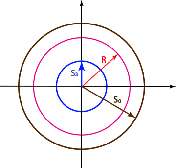
Figure 2: Radius of the Poincaré sphere. The radius $R$ takes its maximum value $S_{0}$ when the decoherence angle $\chi$ is zero. It takes its minimum value $S_{z}$ when $\chi=90^{o}.$ The degree of polarization is maximum when $R=S_{0}$, and is minimum when $R=S_{z}$.

The radius $R$ is the radius of the traditional Poincaré sphere, and is

$$R=\frac{1}{2}\sqrt{(a^{2}-b^{2})^{2}+4(ab)^{2}\cos^{2}\chi}.$$ (42)

with

$$S_{3}=\frac{a^{2}-b^{2}}{2}.$$ (43)

This spherical picture of is traditionally known as the Poincaré sphere [1, 2, 3]

The radius $R$ takes its maximum value $S_{0}$ when $\chi=0^{o}$. It decreases and reaches its minimum value, $S_{3}$, when $\chi=90^{o}$. In terms of $R$, the degree of polarization given in Eq.(37) is

$$f=\frac{R}{S_{0}}.$$ (44)

This aspect of the radius R is illustrated in Fig. 2.

Under the Lorentz transformation, all four Stokes parameters are subject to change. The maximum radius $S_{0}$ and the minimum radius $S_{3}$ do not remain invariant. The radius $R$ is also subject to change. These three radii are illustrated in Fig. 2. While Lorentz transformations shake up these parameters, is there any quantity remaining invariant?

Let us go back to the four-momentum matrix of Eq.(9). Its determinant is $m^{2}$ and remains invariant. Likewise, the determinant of the coherency matrix of Eq.36 should also remain invariant. The determinant in this case is

$$S_{0}^{2}-R^{2}=(ab)^{2}\sin^{2}\chi.$$ (45)

This quantity remains invariant. This aspect is shown on the last row of Table 2.

While the decoherence parameter is not fundamental is influenced by environment, it plays the same mathematical role as in the particle mass which remains as the most fundamental quantity since Isaac Newton, and even after Einstein.

5 Entropy and Feynman’s Rest of the Universe

Another way to measure the lack of coherence is to compute the entropy of the system. The coherency matrix of Eq.(33) leads to the density matrix of the form

$$\rho(\chi)=\frac{1}{a^{2}+b^{2}}\pmatrix{a^{2}&(ab)e^{-i\delta}(\cos\chi)\cr(ab)e^{i\delta}(\cos\chi)&b^{2}},$$ (46)

whose trace is one. This matrix can be diagonalized to

$$\rho(\chi)=\frac{1}{2}\pmatrix{1+f&0\cr 0&1-f},$$ (47)

where $f$ is the degree of polarization given in Eq.(37), which can also be written as

$$f=\frac{\sqrt{\left(a^{2}+b^{2}\right)^{2}-4(ab)^{2}\sin^{2}\chi}}{a^{2}+b^{2}}.$$ (48)

As we noted before, this quantity is one when $\chi=0$ and takes its minimum value when $\chi=90^{o}$.

Then, the entropy becomes

$$S=-\left(\frac{1+f}{2}\right)\ln{\left(\frac{1+f}{2}\right)}-\left(\frac{1-f}{2}\right)\ln{\left(\frac{1-f}{2}\right)}.$$ (49)

The entropy $S$ becomes zero when $\chi=0$. When $\chi=90^{o}$, the entropy takes its maximum value

$$\frac{a^{2}}{a^{2}+b^{2}}\ln{\left(\frac{a^{2}+b^{2}}{a^{2}}\right)}+\frac{b^{2}}{a^{2}+b^{2}}\ln{\left(\frac{a^{2}+b^{2}}{b^{2}}\right)},$$ (50)

In the special case of $a=b$,

$$S=-\left[\cos^{2}\left(\frac{\chi}{2}\right)\right]\ln\left[\cos^{2}\left(\frac{\chi}{2}\right)\right]-\left[\sin^{2}\left(\frac{\chi}{2}\right)\right]\ln\left[\sin^{2}\left(\frac{\chi}{2}\right)\right].$$ (51)

This entropy is a monotonically increasing function. It is zero when $\chi=0$.  Its maximum value is $2\ln(2)$ when $\chi=90^{o}$.

The symmetry between $\cos\chi$ and $\sin\chi$ is well known. Let us now consider another Poincaré sphere where $\cos\chi$ is replaced by $\sin\chi$. Then the density matrix and entropy become

$$\rho^{\prime}(\chi)=\frac{1}{2}\pmatrix{1+f^{\prime}&0\cr 0&1-f^{\prime}},$$

$$S^{\prime}=-\left(\frac{1+f^{\prime}}{2}\right)\ln{\left(\frac{1+f^{\prime}}{2}\right)}-\left(\frac{1-f^{\prime}}{2}\right)\ln{\left(\frac{1-f^{\prime}}{2}\right)},$$ (52)

respectively, with

$$f^{\prime}=\frac{\sqrt{\left(a^{2}-b^{2}\right)^{2}+4(ab)^{2}\sin^{2}\chi}}{a^{2}+b^{2}},$$ (53)

which takes its minimum and maximum values when $\chi=0$ and $\chi=90^{o}$ respectively.

Indeed, $S$ and $S^{\prime}$ move in opposite directions as $\chi$ changes. Thus we are led to consider their addition $\left(S+S^{\prime}\right)$. The question is whether it remains constant. The answer is No. On the other hand, the determinant of the first coherency matrix is $(ab)^{2}\sin^{2}\chi,$ and it is $(ab)^{2}\cos^{\chi}$ for the second determinant. Thus the addition of these two determinants

$$(ab)^{2}\sin^{2}\chi+(ab)^{2}\cos^{\chi}=(ab)^{2}.$$ (54)

is independent of the decoherence angle $\chi$.

While the determinant of is a Lorentz-invariant quantity, there could be a larger group which will change the value of the determinant, thus the decoherence angle. This question has been addressed in the literature [21].

Then there comes the issue of Feynman’s rest of the universe. In his book on statistical mechanics [7], Feynman divides the quantum universe into two systems, namely the world in which we do physics, and the rest of the universe beyond our scope.

However, we could gain a better understanding of physics if we can construct a model of the rest of the universe which can be explained in terms of the physical laws applicable to the world which we observe. With this point in mind, Han et al. considered a system of two coupled world [8]. One of those oscillators belong to the world in which we do physics, while the other is in the rest of the universe. This constitute of an illustrative example of Feynman’s rest of the universe.

In this section, we discussed two Poincaré spheres which are coupled by the addition formula of Eq.(54). One of the spheres talks about the physical world, and the other takes care of the entropy variation of this world through the conservation of Eq.(54). Indeed, these two coupled Poincaré spheres constitute another illustrative example of Feynman’s rest of the universe.

Concluding Remarks

In this report, we noted first that the group of Lorentz transformations can be formulated in terms of two-by-two matrices. This two-by-two formalism can also be used for transformations of the coherency matrix in polarization optics.

Thus, this set of four Stokes parameters is like a Minkowskian four-vector under four-by-four Lorentz transformations. The geometry of the Poincaré sphere can be extended to accommodate this four-dimensional transformations.

It is shown that the decoherence parameter in the Stokes formalism is invariant under Lorentz transformations, like the particle mass in Einstein’s four-vector formalism of the energy and momentum.

Appendix

In Sec. 2, we listed four two-by-two matrices whose repeated applications lead to the most general form of the two-by-two matrix $G$. It is known that every $G$ matrix can be translated into a four-by-four Lorentz transformation matrix through [5, 9, 15]

$$\pmatrix{t^{\prime}+z^{\prime}\cr x^{\prime}-iy^{\prime}\cr x^{\prime}+iy^{\prime}\cr t^{\prime}-z^{\prime}}=\pmatrix{\alpha\alpha^{*}&\alpha\beta^{*}&\beta\alpha^{*}&\beta\beta^{*}\cr\alpha\gamma^{*}&\alpha\delta^{*}&\beta\gamma^{*}&\beta\delta^{*}\cr\gamma\alpha^{*}&\gamma\beta^{*}&\delta\alpha^{*}&\delta\beta^{*}\cr\gamma\gamma^{*}&\gamma\delta^{*}&\delta\gamma^{*}&\delta\delta^{*}}\pmatrix{t+z\cr x-iy\cr x+iy\cr t-z},$$ (55)

and

$$\pmatrix{t\cr z\cr x\cr y}=\frac{1}{2}\pmatrix{1&0&0&1\cr 1&0&0&-1\cr 0&1&1&0\cr 0&i&-i&0}\pmatrix{t+z\cr x-iy\cr x+iy\cr t-z}.$$ (56)

These matrices appear to be complicated, but it is enough to study the our matrices of Eq.(7) and Eq.(8) enough to cover all the matrices in this group. Thus, we give their four-by-four equivalents in this appendix.

$$Z(\delta)=\pmatrix{e^{i\delta/2}&0\cr 0&e^{-i\delta/2}}$$ (57)

leads to the four-by-four matrix

$$\pmatrix{1&0&0&0\cr 1&0&0&0\cr 0&1&\cos\delta&-\sin\delta\cr 0&0&\sin\delta&\cos\delta}.$$ (58)

Likewise,

$$B(\mu)=\pmatrix{e^{\mu/2}&0\cr 0&e^{-\mu/2}}\rightarrow\pmatrix{\cosh\mu&\sinh\mu&0&0\cr\sinh\mu&\cosh\mu&0&0\cr 0&0&1&0\cr 0&0&0&1},$$ (59)

$$R(\theta)=\pmatrix{\cos(\theta/2)&-\sin(\theta/2)\cr\sin(\theta/2)&\sin(\theta/2)}\rightarrow\pmatrix{1&0&0&0\cr 0&\cos\theta&-\sin\theta&0\cr 0&\sin\theta&\cos\theta&0\cr 0&0&0&1},$$ (60)

and

$$S(\lambda)=\pmatrix{\cosh(\lambda/2)&\sinh(\lambda/2)\cr\sinh(\lambda/2)&\sinh(\lambda/2)}\rightarrow\pmatrix{\cosh\lambda&0&\sinh\lambda&0\cr 0&1&0&0\cr\sinh\lambda&0&\cosh\lambda&0\cr 0&0&0&1}.$$ (61)

References

- [1] R. A. M. Azzam and I. Bashara, Ellipsometry and Polarized Light (North-Holland, Amsterdam, 1977).
- [2] M. Born and E. Wolf, Principles of Optics. 6th Ed. (Pergamon, Oxford, 1980).
- [3] C. Brosseau, Fundamentals of Polarized Light: A Statistical Optics Approach (John Wiley, New York, 1998).
- [4] E. Wigner, On unitary representations of the inhomogeneous Lorentz group, Ann. Math. 40, 149-204 (1939).
- [5] M. A. Naimark, Linear Representation of the Lorentz Group, Uspekhi Mat. Nauk 9, No.4(62), 19-93 (1954). An English version of this article (translated by F. V. Atkinson) is in the American Mathematical Society Translations, Series 2. Volume 6, 379-458 (1957).
- [6] M. A. Naimark, Linear Representations of the Lorentz Group, translated by Ann Swinfen and O. J. Marstrand (Pergamon Press, 1964). The original book written in Russian was published by Fizmatgiz (Moscow, 1958).
- [7] R. P. Feynman Statistical Mechanics (Benjamin/Cummings, Reading, Massachusetts, 1972).
- [8] D. Han, Y. S. Kim, and M. E. Noz, Illustrative example of Feynman’s rest of the universe, Am. J. Phys. 67, 61-66 (1999).
- [9] Y. S. Kim and M. E. Noz Theory and Applications of the Poincaré Group (Reidel, Dordrecht 1986).
- [10] D. Han, Y. S. Kim, and D. Son, E(2)-like little group for massless particles and polarization of neutrinos, Phys. Rev. D 26, 3717 - 3725 (1982).
- [11] Y. S. Kim and E. P. Wigner, Space-time geometry of relativistic particles, J. Math. Phys. 31, 55-60 (1990).
- [12] S. Başkal and Y. S. Kim, One analytic form for four branches of the ABCD matrix, J. Mod. Opt. [57], 1251-1259 (2010).
- [13] B. E. A. Saleh and M. C. Teich, Fundamentals of Photonics. 2nd Ed. (John Wiley, Hoboken, New Jersey, 2007).
- [14] D. Han, Y. S. Kim, and M. E. Noz, Jones-matrix formalism as a representation of the Lorentz group, J. Opt. Soc. Am. A 14, 2290-2298 (1997).
- [15] D. Han, Y.S. Kim, and M. E. Noz, Stokes parameters as a Minkowskian four-vector, Phys. Rev. E 56, 6065-76. (1997).
- [16] V. A. Dlugunovich and Y. A. Kurochkin, Vector parameterization of the Lorentz group transformations and polar decomposition of Mueller matrices, Optics and Spectro. 107, 312-17 (2009).
- [17] T. Tudor, Vectorial Pauli algebraic approach in polarization optics. I. Device and state operators, Optik 121, 1226-35 (2010).
- [18] F. I. Fedorov, Vector Parametrization of the Lorentz Group and Relativistic Kinematics, Theo. Math. Physics 2, 248-252 (1970).
- [19] F. I. Fedorov, Lorentz Group (in Russian)(Global Science, Physical-Mathematical Literature, Moscow, 1979).
- [20] S. Baskal and Y. S. Kim, Rotations associated with Lorentz Boosts J. Phys. A: Math. Gen 38 6545–6556 (2005).
- [21] S. Başkal and Y. S. Kim, de Sitter group as a symmetry for optical decoherence, J. Phys. A 39, 7775-88 (2006)