Topology of Fracture Networks

Abstract

We propose a mapping from fracture systems consisting of intersecting fracture sheets in three dimensions to an abstract network consisting of nodes and links. This makes it possible to analyze fracture systems with the methods developed within modern network theory. We test the mapping for two-dimensional geological fracture outcrops and find that the equivalent networks are small-world and dissasortative. By anlayzing the Discrete Fracture Network model, which is used to generate artifical fracture outcrop networks, we also find small world networks. However, the networks turn out to be assortative.

Topological analysis of networks has had an explosive growth over the last decade b03 . A large number of new concepts and quantitive tools for describing networks have been introduced, making it possible to describe and classify complex network structures at a level that never earlier has been achieved ab02 ; blmch06 . There is one class, though, of networks that has resisted this kind of analysis: Fracture networks. These consist of intersecting fracture sheets, making both the concepts of links and nodes far from obvious. Fracture networks, however, are extremely important from a technological point of view. For example, in carbonate petroleum reservoirs, the oil is transported through fracture networks as the permeability of the porous matrix is too low g07 . Another example is the extraction of shale gas though hydrofracturing m11 .

We propose a transformation from fracture network to an equivalent network consisting of nodes and links. This makes it possible to qualitatively and quantitatively characterize the topology of fracture networks.

An important consequence of this is that it is possible to compare models that generate artificial networks with real networks quantitatively.

Fracture outcrop networks have been studied from a network point of view by Valentini et al. vpp07a ; vpp07b . Fracture outcrops are fracture lines visible on the surfaces of geological formations. The outcrop fracture lines are one-dimensional cuts through the two-dimensional fracture sheets. Valentini et al. treats fracture lines as links and their crossing points as nodes, this gives a more narrow degree distribution than the transform proposed in this paper. However, Valentini et al. also conclude that fracture networks are small-world networksvpp07a . In three dimensions where the fractures are sheets, the transformation we propose is necessary to define the topology network.

Our analysis is somewhat related to the information measure for cities introduced by Rosvall et al. rtms05 .

Figure 1: (Color online) a) Fracture network of outcrop AMS000025 b) Equivalent network based on the original network shown in a).

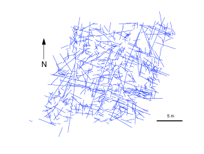
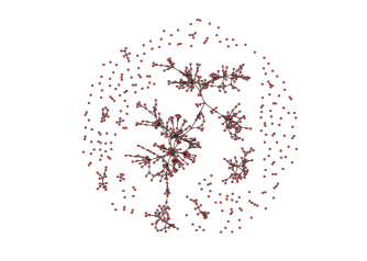
Lacking data on three-dimensional fracture systems, we analyse in the following fracture data from eight outcrops found in south-east Sweden. A detailed description of the bedrock composition and geological history are given in (sasw08, ; ddbd06, ). We show one of the outcrop fracture networks in Fig. 1a. As we shall see, the equivalent network (shown in Fig. 1b) constructed from the original network has small-world character. Furthermore, it is disassortative.

We then go on to analyse artificial fracture networks generated with the Discrete Fracture Network (DFN) model dbdd03 . The equivalent networks constructed from the original networks generated by this model also show small-world behavior. However, they are assortative.

Figure 2: (Color online) Clock-wise from upper left. a) Representation of fracture outcrop network. b) Reconnected fracture network. c) Equivalent network placed on top of fracture outcrop network. d) Equivalent network representation of b).

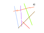
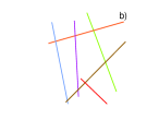
The eight outcrops covers between 250 and 600 $\textrm{m}^{2}$. All visible fractures with length over 0.5 m have been recorded in the data sets. We prepare the data sets as follows. When tracing the fracture lines, they may appear disconnected or doubled due to topography or ground weathering. An illustration of a outcrop is shown in Fig. 2a. We therefore use a reconnection procedure ddgdb09 . That is, we first project fracture traces on a flat surface to reduce the perturbation due to rock surface topography. Then scattered segments that are likely to belong to the same trace are reconnected to one single segment accounting for orientation and distance consistency. We focus on traces with a dashed-line, disconnected step or layered patterns. We then straighten all the fractures lines. The result is shown in Fig. 2b.

Figure 3: (Color online) Cumulative degree distribution for: a) Networks generated from the eight outcrop data sets. Insert shows the average compared to a log-log (exponent $-2.3$) and a log-normal fit. b) DFN model. Values for the expoents of the fits are given in Table 2.

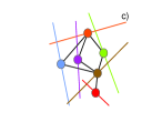
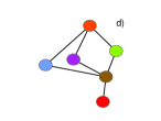
We have now come to the central idea of this paper. In Fig. 2c, each fracture line has been associated with a node. Whenever two fracture lines cross, we place a link between the nodes representing the two fracture lines. In Fig. 2d, we show the equivalent network consisting of nodes representing the fracture lines and links representing crossing fracture lines a08 .

We note that this equivalent network is as simple to construct in a three-dimensional system of fracture sheets: each fracture sheet is represented by a node and whenever two sheets cross each other, a link is placed between the equivalent nodes.

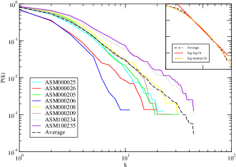
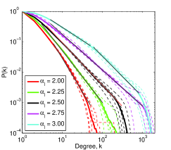
Arguably the most central property of any complex network is the degree distribution $p(k)$. The degree, $k$, of a node is the number of other nodes that it is linked to. The equivalent networks generated from the outcrop networks show a broad degree distribution. We plot the cumulative distribution, $P(k)$ in Fig. 3. When $P(k)$ follows a power-law the network is scale free ab02 . We plot the data against log-log fits, but note that our geological data can be well fited by a log-normal. In the case of the DFN data the goodness of the log-log fit is dependent on model parameters.

The clustering is a local measure of how well a network is connected on a local neighbor-to-neighbor scale. The global clustering coefficient, $C$, is defined ws98 ; n03 as the average over all the local clustering coefficients, $C_{i}$, for each node

$$C=\frac{1}{N}\sum_{i=1}^{i=N}C_{i}=\frac{1}{N}\sum_{i=1}^{i=N}\frac{2E_{NN,i}}{k_{i}(k_{i}-1)},$$ (1)

where $k_{i}$ is the degree of node $i$, $N$ is the total number of nodes and $E_{NN,i}$ is the number of links between the nearest neighbors of node $i$. The clustering coefficient falls in the interval $0\leq C\leq 1$, and a high value indicates that there is a high chance that two neighbors of a node is connected to each other. This makes the network highly connected on a local scale, making it easy for nodes to efficiently interact on this scale.

Table 1: List of the number of nodes (fractures), links, maximum degree $k_{max}$, average degree $\bar{k}$, clustering coefficient $C$, clustering coefficient for rewired networks $C_{RW}$, clustering coefficient for random networks $C_{RA}$, efficiency $E$, efficiency for rewired networks $E_{RW}$, and efficiency for random networks $E_{RA}$ for all the outcrop samples.

Sample	Nodes	Links	$k_{max}$	$\bar{k}$	$C$	$C_{RW}$	$C_{RA}$	$E$	$E_{RW}$	$E_{RA}$
AMS000025	787	858	23	2.18	0.170	0.0048	0.00178	0.046	0.104	0.101
AMS000026	716	520	20	1.45	0.088	0.0033	0.00087	0.019	0.048	0.032
AMS000205	973	1188	32	2.44	0.193	0.0043	0.00174	0.032	0.122	0.118
AMS000206	737	487	11	1.32	0.120	0.0013	0.00067	0.004	0.033	0.020
AMS000208	955	1297	31	2.72	0.226	0.0067	0.00213	0.079	0.138	0.138
AMS000209	955	1162	27	2.43	0.177	0.0050	0.00178	0.068	0.119	0.118
AMS100234	946	1549	44	3.27	0.236	0.0138	0.00291	0.133	0.164	0.172
AMS100235	785	1392	44	3.55	0.243	0.0180	0.00394	0.141	0.176	0.192
Average	857	1057	29	2.42	0.182	0.0072	0.00198	0.065	0.113	0.111

In order to determine whether the clustering coefficients found for the networks are large for their number of nodes and links, we compare them to rewired and random versions of the same networks. In rewiring mg01 two pairs of connected nodes are selected at random, and the links interchanged so that two new pairs of connected nodes are created. The procedure is repeated until all links are moved. This preserves the degree distribution since all nodes retain their initial degree, but it removes any correlation between the degrees of the connected nodes. For the random version all links are removed and redistributed randomly between the nodes. This produces a new degree distribution that is generally not broad. In all cases the quoted values for these networks are averaged over 1000 realizations. As can be seen from Table 1, the equivalent networks have an average clustering coefficient of 0.18 which is more than an order of magnitude larger than for comparable rewired networks, and two orders of magnitude larger than for purely random versions. Hence, they are well connected on a local scale.

The efficiency, $E$, is a global measure for how well the different parts of the network are connected, and how easily nodes in different parts of the network can interact. The measure is defined using the shortest distance, $d_{ij}$, between two nodes $i$ and $j$ blmch06

$$E=\frac{1}{N(N-1)}\sum_{(i,j)\in N,i\neq j}\frac{1}{d_{ij}},$$ (2)

where $d_{ij}=\infty$ if node $i$ and $j$ are not connected. $E$ falls in the interval $0\leq E\leq 1$, and a high value indicates that it is easy for nodes far apart in the network to interact since there on average is just a few links between any two nodes.

In Table 1 we present $E$ for all the equivalent networks and their average is 0.065, which is smaller than for the rewired ($E_{RW}$) and random ($E_{RA}$) versions both having an average of 0.11. However the efficiency ($E$) is only smaller by a factor of about 2, making $E$ and $E_{RW/RA}$ of the same order. We would expect the rewired and random networks to have a high efficiency, several orders of magnitude larger than ordered networks, because they have a large portion of long-range links. The fact that the equivalent networks have an efficiency comparable to that of the rewired and random versions means that compared to ordered networks they have a large efficiency. We will discuss the impact of $C$ and $E$ for the equivalent networks in more detail below.

Figure 4: (Color online) Plot of the correlation matrix $C(k_{1},k_{2})$ based on the equivalent networks generated from the eigth outcrop fracture data sets.

It is also interesting to study any correlations between the degrees of linked nodes. Does high degree nodes link predominantly to low degree nodes or high degree nodes? Maslov and Sneppen (ms02, ) introduced a correlation matrix

$$C(k_{1},k_{2})=\frac{P(k_{1},k_{2})}{P_{R}(k_{1},k_{2})},$$ (3)

where $P(k_{1},k_{2})$ is the probability that a node of degree $k_{1}$ is linked to a node of degree $k_{2}$ for the network to be investigated. $P_{R}(k_{1},k_{2})$ is the same probability of a rewired version of the network. If $C(k_{1},k_{2})=1$ for all $(k_{1},k_{2})$ then there is no degree correlations in the linking between nodes. If $C(k_{1},k_{2})>1$ for some values of $(k_{1},k_{2})$ then there is an over-representation of links between nodes of degree $k_{1}$ and $k_{2}$ in the investigated network compared to that of a rewired version of the network. If $C(k_{1},k_{2})<1$ there is an under-representation. Note that the matrix $C(k_{1},k_{2})$ is symmetric.

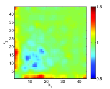
In Fig. 4 we have plotted the average of the matrix $C(k_{1},k_{2})$ for all outcrops, where $P_{R}(k_{1},k_{2})$ is averaged over 10000 realizations. We observe an over-representation of small degree nodes linking to higher degree nodes, and an under-representation of equal degree nodes linking to each other. Such networks are disassortative, and are abundant in naturally occurring networks (rt04, ; hh07, ).

The characteristic path length, $L$ is defined as the average distance between any pair of nodes of a network,

$$L=\frac{1}{N(N-1)}\sum_{(i,j)\in\textit{N},i\neq j}d_{ij}.$$ (4)

Having a large clustering coefficient indicates a large local connectivity, and a small characteristic path length indicates a large global connectivity. When both of these criteria are fulfilled, we have a small-world network ws98 . Networks consisting of more than one disjoint part will have $d_{ij}=\infty$ for at least one pair of nodes. Hence, the characteristic path length is not a good measure for the global connectivity of such networks. However a small value of $d_{ij}$ for most pairs of nodes will give a large average value for $1/d_{ij}$ which is measured by the efficiency. Therefore a large $E$ is comparable to a small $L$ for describing the global connectedness. Since the fracture networks found in the outcrops have been shown to have a clustering coefficient significantly larger than rewired and random versions, and an efficiency of the same order as the rewired and random networks we conclude that these are small-world networks.

Figure 5: (Color online) Examples of fracture systems generated with the DFN model for varying parameters $\alpha_{l}$ and $D_{2}$.

We now turn to analyzing the DFN model dbdd03 . It is based on the observation that the length of fracture lines in outcrops, $l$, are distributed according to a power law r99 ; bbod01

$$p(l)\sim l^{-\alpha_{l}}\;.$$ (5)

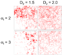
The outcrops can be divided into two groups: one with $\alpha_{l}=3$ (ASM000205 and ASM000206) and one with $\alpha_{l}=2.3\pm 0.2$ (the rest) dgdbdm10 . The angular distribution of the directions of the fractures depends on the fracture system. We assume here the simplest, i.e., a uniform distribution. The outcrop data studied show strong signs of prefered directions for the fractures, but using this in the angular distribution of the DFN model does not have a significant impact. Lastly, the position of the fractures must be specified. The DFN model uses a hierarchical construction sl87 ; m91 to place the midpoints of the fractures on a fractal set characterized by a fractal dimension $D_{2}$. We show in Fig. 5 the resulting fracture systems for different parameters $\alpha_{l}$ and $D_{2}$. The outcrop data has $D_{2}\approx 2$. Further details may be found in dgdbdm10 .

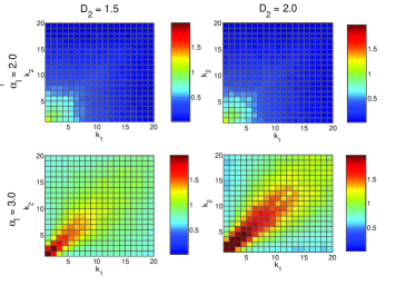
The results of analyzing the equivalent networks of the DFN model networks are given in Table 2. The data are based on 1000 networks of comparable size to those in the outcrop fracture data sets. From the table, we see the same trends as those observed in Table 1 for the eight outcrop fracture data sets and it is possible to find a combination of $\alpha_{l}$ and $D_{2}$ to make match between them. However, we show in Fig. 6 the averaged degree correlation matrix. This indicates an assortative network structure: nodes of equal coordination number tend to be connected. This is the opposite of what is observed for the outcrop data sets, see Fig. 4. Hence, the topology of the artifical networks is quite different from the natural ones. This implies that the topology of the fracture network themselves, artifical and real, are quite different. This difference is not visible from direct observation.

Hence, by constructing the equivalent networks, we have access to the entire analysis toolbox of modern network theory for fracture networks. As we have shown in the analysis presented, this makes it possible to test fracture network models on a quantitative level beyond what has been possible earlier.

Figure 6: The degree correlation matrix $C(k_{1},k_{2})$ for different DFN model parameters $\alpha_{l}$ and $D_{2}$. This figure should be compared with Fig. 4.

Table 2: List of degree distribution power-law exponents $\alpha_{k}$, clustering coefficient C, clustering coefficient for rewired networks $C_{RW}$, clustering coefficient for comparable random networks $C_{RA}$, efficiency E, efficiency for rewired networks $E_{RW}$, and efficiency for comparable random networks $E_{RA}$ for various fracture length power-law exponents $\alpha_{l}$.

$\alpha_{l}$	$\alpha_{k}$	$C$	$C_{RW}$	$C_{RA}$	$E$	$E_{RW}$	$E_{RA}$
2.00	2.2	0.08	0.019	0.047	0.028	0.042	0.11
2.25	1.7	0.11	0.013	0.031	0.027	0.049	0.11
2.50	1.4	0.17	0.013	0.019	0.037	0.083	0.10
2.75	1.2	0.26	0.014	0.014	0.050	0.134	0.09
3.00	0.9/1.3	0.31	0.013	0.008	0.050	0.154	0.07

We thank Svensk Kärnbränslehantering AB for outcrop data, H. F. Hansen and E. Skjetne for discussions and the referees for valuable comments. C. A. A. and A. H. thank Statoil and The Norwegian Academy of Science and Letters for funding through their VISTA program. S. M. H. and A. H. thank the Norwegian Research Council for funding through the CLIMIT program, grant no. 199970.

References

- (1) A. L. Barabási, Linked (Plume, New York, 2003).
- (2) R. Albert and A. L. Barabási, Rev. Mod. Phys. 74, 47 (2002).
- (3) S. Boccaletti, V. Latora, Y. Moreno, M. Chavez and D. U. Hwang, Phys. Rep. 424, 175 (2006).
- (4) T. D. Van Golf-Racht, Develop. Petr. Sci. 44, 683 (2007).
- (5) C. Mooney, Sci. Am. 305 (5), 80 (2011).
- (6) L. Valentini, D. Perugini and G. Poli, Physica A, 377, 323 (2007).
- (7) L. Valentini, D. Perugini and G. Poli, J. Volcanol. Geotech. Res. 159, 355 (2007).
- (8) M. Rosvall, A. Trusina, P. Minnhagen and K. Sneppen, Phys. Rev. Lett. 94, 028701 (2005).
- (9) A. Ström, J. Andersson, K. Skagius and A. Winberg, Appl. Geochem. 23, 1747 (2008).
- (10) C. Darcel, P. Davy, O. Bour and J. R. de Dreuzy, Swedish Nuclear Fuel and Waste Management, R-06-79 (2006).
- (11) C. Darcel, O. Bour, P. Davy and J. R. de Dreuzy, Water Res. Res. 39, 1272 (2003).
- (12) C. Darcel, P. Davy, R. Le Goc, J. R. de Dreuzy and O. Bour, Swedish Nuclear Fuel and Waste Management, R-09-38 (2009).
- (13) C. A. Andresen, Ph. D. thesis, NTNU (2008).
- (14) D. J. Watts and S. H. Strogatz, Nature, 393, 440 (1998).
- (15) M. E. J. Newman, SIAM Rev. 45, 167 (2003).
- (16) N. Mathias and V. Gopal, Phys. Rev. E, 63, 021117 (2001).
- (17) S. Maslov and K. Sneppen, Science, 296, 910 (2002).
- (18) Virtual Round Table on Ten Leading questions for network Research, Eur. Phys. J. B 38, 143 (2004).
- (19) H. F. Hansen and A. Hansen, Physica A, 377, 698 (2007).
- (20) C. E. Renshaw, Water Res. Res. 35, 2661 (1999).
- (21) E. Bonnet, O. Bour, N. E. Odling and P. Davy, Rev. Geophys. 39, 347 (2001).
- (22) P. Davy, R. Le Goc, C. Darcel, O. Bour, J. R. de Dreuzy and R. Munier, J. Geophys. Res. 115, B10411 (2010).
- (23) D. Schertzer and S. Lovejoy, J. Geophys. Res. 92, 9693 (1987).
- (24) P. Meakin, Physica A, 173, 305 (1991).