Geometry, mixing properties and hypocoercivity of a degenerate diffusion arising in technical textile industry

Martin Grothaus Martin Grothaus, Mathematics Department, University of Kaiserslautern,
P.O.Box 3049, 67653 Kaiserslautern, Germany.
Email: grothaus@mathematik.uni-kl.de,
Functional Analysis and Stochastic Analysis Group,
URL: http://www.mathematik.uni-kl.de/similar-to\simwwwfktn/
Axel Klar Axel Klar, Mathematics Department, University of Kaiserslautern,
P.O.Box 3049, 67653 Kaiserslautern, Germany.
Email: klar@mathematik.uni-kl.de,
Technomathematics Group,
URL: http://wwwagtm.mathematik.uni-kl.de/agtm/
Johannes Maringer Johannes Maringer, Mathematics Department, University of Kaiserslautern,
P.O.Box 3049, 67653 Kaiserslautern, Germany.
Email: maringer@itwm.fraunhofer.de,
Technomathematics Group,
URL: http://wwwagtm.mathematik.uni-kl.de/agtm/
 and  Patrik Stilgenbauer Patrik Stilgenbauer, Mathematics Department, University of Kaiserslautern,
P.O.Box 3049, 67653 Kaiserslautern, Germany.
Email: stilgenb@mathematik.uni-kl.de,
Functional Analysis and Stochastic Analysis Group,
URL: http://www.mathematik.uni-kl.de/similar-to\simwwwfktn/
(Date: March 18, 2024)
Abstract.

We study a stochastic equation modeling the lay-down of fibers in the production process of nonwovens. The equation can be formulated as some manifold-valued Stratonovich stochastic differential equation living on d×𝕊d1superscript𝑑superscript𝕊𝑑1\mathbb{R}^{d}\times\mathbb{S}^{d-1}, d2𝑑2d\geq 2. Especially, we study the long time behaviour of the stochastic process. Demanding mathematical difficulties arising due to the degeneracity of the lay-down equation and its associated generator. We prove strong mixing properties by making use of the hypoellipticity of the generator and a new version of Doob’s theorem derived recently in [GN12]. Moreover, we show convergence to equilibrium exponentially fast with explicitly computable rate of convergence. This analytic approach uses powerful modern Hilbert space methods from the theory of hypocoercivity developed in [DMS10]. Summarizing, we give interesting mathematical applications of geometric stochastic analysis to real world problems.

Key words and phrases:
Convergence to equilibrium; Strong mixing property; Hypocoercivity; Exponential rate of convergence; Ergodicity; Stratonovich SDEs on manifolds; Fiber dynamics; Geometric modeling; Hypoelliptic operator; Degenerate diffusion
2000 Mathematics Subject Classification:
Primary 37A25; Secondary: 58J65; Secondary; 47A35; Secondary 60H30; Secondary 60D05;

1. Introduction

This article is about the mathematical analysis of new fiber lay-down equations developed recently in [KMW12]. Herein fiber lay-down processes arise in the production process of nonwovens and the expression is used for the description of the forms generated by the stochastic lay-down of flexible fibers. The understanding, optimization and mathematical simulation of such fiber webs is of great industrial interest, we refer to [KMW09] and references therein. Areas of application where these stochastic lay-down processes can be observed include e.g. composite materials (filters), textiles, as well as the hygiene industry. In [MW06] a general mathematical model describing the full fiber spinning process is introduced and is nowadays implemented in the software tool FYDIST developed at the Fraunhofer ITWM, Kaiserslautern. Nevertheless, the numerical simulation leads to excessively large computation times. Hence it would be desirable to have simplified stochastic models at hand simulating a virtual fiber web in a fast and efficient way. The first of such surrogate models, the basic two-dimensional model, is developed in [GKMW07] and reads as some Itô stochastic differential equation (SDE) in 3superscript3\mathbb{R}^{3} of the form

dξt=τ(αt)dtdsubscript𝜉𝑡𝜏subscript𝛼𝑡dt\displaystyle\mathrm{d}\xi_{t}=\tau(\alpha_{t})\,\mathrm{dt} (1.1)
dαt=Φ(ξt)τ(αt)dt+σdWt.dsubscript𝛼𝑡Φsubscript𝜉𝑡superscript𝜏bottomsubscript𝛼𝑡dt𝜎dsubscript𝑊𝑡\displaystyle\mathrm{d}\alpha_{t}=-\nabla\Phi(\xi_{t})\cdot\tau^{\bot}(\alpha_{t})\,\mathrm{dt}+\sigma\,\mathrm{d}W_{t}.

Here τ(α)=(cos(α),sin(α))T𝜏𝛼superscript𝛼𝛼𝑇\tau(\alpha)=(\cos(\alpha),\sin(\alpha))^{T}, τ=ταsuperscript𝜏bottom𝜏𝛼\tau^{\bot}=\frac{\partial\tau}{\partial\alpha}, σ𝜎\sigma is a nonnegative constant and W𝑊W is a standard one-dimensional Brownian motion. Φ:2:Φsuperscript2\Phi:\mathbb{R}^{2}\rightarrow\mathbb{R} is a suitable function called the potential. This basic model has been extended in [KMW12] to the more realistic three-dimensional case which serves as starting point for all our mathematical studies in the underlying article. And exactly this extension to the three-dimensional case requires the usage of a differentialgeometric language.

At first we discuss the geometry underlying the previously mentioned equation introduced in [KMW12]. Starting with the two-dimensional model (1.1) we present a new differential geometric derivation and formulation of the model from [KMW12] in each dimension d𝑑d\in\mathbb{N}, d2𝑑2d\geq 2. Therefore we formulate Equation (1.1) first in its most natural way on 2×/2πsuperscript22𝜋\mathbb{R}^{2}\times\mathbb{R}/{2\pi\mathbb{Z}}. The latter space is diffeomorphic to 2×𝕊1superscript2superscript𝕊1\mathbb{R}^{2}\times\mathbb{S}^{1} where 𝕊𝕊\mathbb{S} stands as usual for the unit sphere. Consequently, we get the analogue equation of (1.1) living on 2×𝕊1superscript2superscript𝕊1\mathbb{R}^{2}\times\mathbb{S}^{1}. The resulting equation can then directly be translated to higher dimensions and yields the final d𝑑d-dimensional fiber lay-down model given as some manifold-valued Stratonovich SDE with state space d×𝕊d1superscript𝑑superscript𝕊𝑑1\mathbb{R}^{d}\times\mathbb{S}^{d-1} by

dξt=vtdtdsubscript𝜉𝑡subscript𝑣𝑡dt\displaystyle\mathrm{d}\xi_{t}=v_{t}\,\mathrm{dt} (1.2)
dvt=(Ivtvt)Φ(ξt)dt+σ(Ivtvt)dWt.dsubscript𝑣𝑡𝐼tensor-productsubscript𝑣𝑡subscript𝑣𝑡Φsubscript𝜉𝑡dt𝜎𝐼tensor-productsubscript𝑣𝑡subscript𝑣𝑡dsubscript𝑊𝑡\displaystyle\mathrm{d}v_{t}=-(I-v_{t}\otimes v_{t})\nabla\Phi(\xi_{t})\,\mathrm{dt}+\sigma\,(I-v_{t}\otimes v_{t})\circ\mathrm{d}W_{t}.

Here xy=xyTtensor-product𝑥𝑦𝑥superscript𝑦𝑇x\otimes y=xy^{T}, ΦC(d)Φsuperscript𝐶superscript𝑑\Phi\in C^{\infty}(\mathbb{R}^{d}) and W𝑊W is a standard d𝑑d-dimensional Brownian motion, see Section 3 for details. This precise fomulation is also necessary for all the forthcoming analysis and we strongly believe that the geometric derivation can be helpful for every applied mathematician who aims to derive similiar manifold-valued stochastic equations. Furthermore, we provide concret numerical simulation formulas of (1.2) in specific local coordinate systems, so called local SDEs. As consequence, for d=2𝑑2d=2 we obtain back (1.1) and for d=3𝑑3d=3 the local SDE reduces to the three-dimensional model derived in [GKMW07]. We finish the geometric discussion in Section 4. Therein we further discuss basic existence statements of all occuring stochastic equations by constructing global solutions to the basic two-dimensional model (1.1) with state space 3superscript3\mathbb{R}^{3} and the general geometric fiber lay-down model (1.2) living on d×𝕊d1superscript𝑑superscript𝕊𝑑1\mathbb{R}^{d}\times\mathbb{S}^{d-1}.

Of course, the cases d=2𝑑2d=2 and d=3𝑑3d=3 are the physical relevant ones. Nevertheless, for all the forthcoming analysis, it is elegant to study Equation (1.2) in its general mathematical form. We emphasize that our upcoming stochastic and functionalanalytic considerations of the d𝑑d-dimensional fiber lay-down model are done in a coordinate free way.

The density of the stochastic process solving (1.2) satisfes the associated Fokker-Planck evolution equation. An important criterion for the quality of the fiber web and the resulting nonwoven material is how fast the process converges towards its stationary state. Of essential interest is therefore the speed of convergence. Moreover, from a practical point of view, process parameters should be adjusted in order to obtain optimal convergence to equilbrium.

This motivates that we devote the main interest in the underlying paper to the study of the long-time behaviour of the d𝑑d-dimensional fiber lay-down equation. Demanding mathematical difficulties are then occuring due to the degeneracity of (1.2). The convergence to equilibrium of the „flat“ two-dimensional fiber lay-down model is already analyzed in several articles. Basing upon the theory of Dirichlet forms and operator semigroups, the approach of [GK08] gives an ergodic theorem and establishes explicit rates of convergence. The underlying object of study therein is the two-dimensional fiber lay-down Kolmogorov PDE and its corresponding Kolmogorov operator. Another approach is presented in [DKMS12]. There the authors analyze the two-dimensional fiber lay-down Fokker-Planck PDE together with its associated generator and prove convergence to equilibrium with an exponential, explicitly computable rate of convergence. This approach uses modern methods from [DMS10] in which a new hypocoercivity theory in a Hilbert space setting is developed. For a general study of the theory of hypocoercivity, the reader may consult [Vil09]. Finally, the quite recently published article [KSW11] uses a probabilistic approach. The authors are able to derive strong mixing properties under weak assumptions on the potential and, assuming some stronger conditions, they can prove geometric ergodicity of the two-dimensional fiber lay-down process.

In Section 5 we start studying the long time behaviour of our general, geometric d𝑑d-dimensional fiber lay-down process by proving strong mixing properties, see Theorem 5.3. The approach is disjoint and different to the one given in the two-dimensional setting in [KSW11], and moreover, it has even been developed at the same time independently. Our approach works for smooth potentials ΦΦ\Phi. This is a slightly stronger assumption as made in [KSW11] in the two-dimensional case. Nevertheless, our strategy applies to the full manifold-valued d𝑑d-dimensional fiber lay-down SDE containing especially the two-dimensional situation. We make use of a new version of Doob’s theorem, see [GN12], which perfectly fits into the fiber lay-down setting.

Afterwards, we switch to functional analysis and apply the fascinating and powerful hypocoercivity theory from [DMS10] once more, see Section 6. We generalize the strategy in [DKMS12] to the d𝑑d-dimensional setting requiring some differential geometric tools. The object of interest in this section is the hypoelliptic Kolmogorov operator associated to (1.2) given by

L𝐿\displaystyle L =vξ(Ivv)Φ(ξ)v+σ22Δ𝕊d1absent𝑣subscript𝜉𝐼tensor-product𝑣𝑣Φ𝜉subscript𝑣superscript𝜎22subscriptΔsuperscript𝕊𝑑1\displaystyle=v\cdot\nabla_{\xi}-(I-v\otimes v)\nabla\Phi(\xi)\cdot\nabla_{v}+\frac{\sigma^{2}}{2}\,\Delta_{\mathbb{S}^{d-1}}

which is analyzed in an appropriately chosen L2superscript𝐿2L^{2}-space. In particular, we make use of modern entropy methods. We obtain convergence to equilibrium exponentially fast with explicitly computable rate of convergence, see Theorem 6.4.

Moreover, in Section 2 we introduce some basic geometric language and give a short introduction to the concept of manifold-valued Stratonovich SDEs. Further useful statements needed for our analysis are proven in the Appendix.

Finally, the progress achieved in this paper may be summarized by the following list of main results:

  • Differential geometric derivation and formulation of the fiber lay-down model in each dimension as some manifold-valued Stratonovich SDE.

  • Construction of strong solutions to all occuring fiber lay-down equations.

  • Strong mixing properties of the geometric fiber lay-down process under weak assumptions on the potential, see Theorem 5.3, by making use of a new version of Doob’s theorem proven in [GN12].

  • Exponential convergence to equilibrium of the geometric fiber lay-down process towards a unique stationary state with explicitly computable rate of convergence, see Theorem 6.4. Here we use modern Hilbert space methods from the theory of hypocoercivity developed in [DMS10].

2. Setup and Notations

Before starting we introduce some notations, fix the language concerning the d𝑑d-sphere and give a short introduction to the concept of Stratonovich stochastic differential equations (SDEs) on manifolds. Until the end of this article we follow the notations and language introduced in the underlying section without further mention this again.

C(𝕏)superscript𝐶𝕏C^{\infty}(\mathbb{X}) denotes the set of all infinitely often differentiable functions f:𝕏:𝑓𝕏f:\mathbb{X}\rightarrow\mathbb{R} on some differentiable manifold 𝕏𝕏\mathbb{X}. The index c𝑐c indicates compact support. \nabla (or also denoted by xsubscript𝑥\nabla_{x} or dsubscriptsuperscript𝑑\nabla_{\mathbb{R}^{d}}) always denotes the usual gradient operator in dsuperscript𝑑\mathbb{R}^{d}, d𝑑d\in\mathbb{N}, (with respect to the variable x𝑥x) as column vector. |||\cdot| is the standard euclidean norm. The standard euclidean scalar product is simply denoted by \cdot or also by (,)eucsubscripteuc\left(\cdot,\cdot\right)_{\text{euc}}. Superscript T𝑇T denotes the transpose of some matrix. The expression smooth means that the underlying object is of class Csuperscript𝐶C^{\infty}. I𝐼I is the identity matrix. Partial derivatives in dsuperscript𝑑\mathbb{R}^{d} with respect to some variable x𝑥x are denoted as usual by x𝑥\frac{\partial}{\partial x} or for short by xsubscript𝑥\partial_{x}. Convention: Any vector xd𝑥superscript𝑑x\in\mathbb{R}^{d} is always understood as column vector. And the notation (x,y)𝑥𝑦(x,y) for xd𝑥superscript𝑑x\in\mathbb{R}^{d}, yk𝑦superscript𝑘y\in\mathbb{R}^{k}, is understood as column vector.

Next let us fix some geometric language. Let d𝑑d\in\mathbb{N}. We consider the d𝑑d-sphere given by 𝕊d={vd+1||v|2=1}superscript𝕊𝑑conditional-set𝑣superscript𝑑1superscript𝑣21\mathbb{S}^{d}=\{v\in\mathbb{R}^{d+1}\leavevmode\nobreak\ |\leavevmode\nobreak\ |v|^{2}=1\}. The algebraic tangent space Tv𝕊dsubscript𝑇𝑣superscript𝕊𝑑T_{v}\mathbb{S}^{d} at the point v𝕊d𝑣superscript𝕊𝑑v\in\mathbb{S}^{d} can naturally be embedded into d+1superscript𝑑1\mathbb{R}^{d+1}. Under this identification any \mathbb{R}-derivation DTv𝕊d𝐷subscript𝑇𝑣superscript𝕊𝑑D\in T_{v}\mathbb{S}^{d}, v𝕊d𝑣superscript𝕊𝑑v\in\mathbb{S}^{d}, corresponds to some Ad+1𝐴superscript𝑑1A\in\mathbb{R}^{d+1} with (A,v)euc=0subscript𝐴𝑣euc0\left(A,v\right)_{\text{euc}}=0. We canonically identify D𝐷D and A𝐴A, in notation DA𝐷𝐴D\equiv A. For fC(𝕊d)𝑓superscript𝐶superscript𝕊𝑑f\in C^{\infty}(\mathbb{S}^{d}) it holds Df=Ad+1f~(v)𝐷𝑓𝐴subscriptsuperscript𝑑1~𝑓𝑣Df=A\cdot\nabla_{\mathbb{R}^{d+1}}\widetilde{f}(v) where f~~𝑓\widetilde{f} is any smooth extension of f𝑓f defined in an open neighbourhood in d+1superscript𝑑1\mathbb{R}^{d+1} of v𝑣v. So this justifies the notation Af=Avf(v)𝐴𝑓𝐴subscript𝑣𝑓𝑣Af=A\cdot\nabla_{v}f(v) instead of Df𝐷𝑓Df. Moreover, for a given smooth vector field 𝒜𝒜\mathcal{A} on 𝕊dsuperscript𝕊𝑑\mathbb{S}^{d} defined by 𝕊dv𝒜(v)Tv𝕊dcontainssuperscript𝕊𝑑𝑣maps-to𝒜𝑣subscript𝑇𝑣superscript𝕊𝑑\mathbb{S}^{d}\ni v\mapsto\mathcal{A}(v)\in T_{v}\mathbb{S}^{d}, we write 𝒜f(v)=𝒜(v)f𝒜𝑓𝑣𝒜𝑣𝑓\mathcal{A}f(v)=\mathcal{A}(v)f, fC(𝕊d)𝑓superscript𝐶superscript𝕊𝑑f\in C^{\infty}(\mathbb{S}^{d}). The spherical gradient of such an f𝑓f is denoted by grad𝕊dfsubscriptgradsuperscript𝕊𝑑𝑓\text{grad}_{\mathbb{S}^{d}}f. One has

grad𝕊df(v)=(Ivv)d+1f~(v),fC(𝕊d),v𝕊d.formulae-sequencesubscriptgradsuperscript𝕊𝑑𝑓𝑣𝐼tensor-product𝑣𝑣subscriptsuperscript𝑑1~𝑓𝑣formulae-sequence𝑓superscript𝐶superscript𝕊𝑑𝑣superscript𝕊𝑑\displaystyle\text{grad}_{\mathbb{S}^{d}}f(v)=(I-v\otimes v)\,\nabla_{\mathbb{R}^{d+1}}\widetilde{f}(v),\leavevmode\nobreak\ f\in C^{\infty}(\mathbb{S}^{d}),\leavevmode\nobreak\ v\in\mathbb{S}^{d}.

Here xy:=xyTassigntensor-product𝑥𝑦𝑥superscript𝑦𝑇x\otimes y:=xy^{T}, x,yd+1𝑥𝑦superscript𝑑1x,y\in\mathbb{R}^{d+1} and f~~𝑓\widetilde{f} is chosen as before. This definition is again independent of the local smooth extension f~~𝑓\widetilde{f} for f𝑓f. In short notation we also write grad𝕊df(v)=(Ivv)vf(v)subscriptgradsuperscript𝕊𝑑𝑓𝑣𝐼tensor-product𝑣𝑣subscript𝑣𝑓𝑣\text{grad}_{\mathbb{S}^{d}}f(v)=(I-v\otimes v)\,\nabla_{v}f(v) for fC(𝕊d)𝑓superscript𝐶superscript𝕊𝑑f\in C^{\infty}(\mathbb{S}^{d}) and v𝕊d𝑣superscript𝕊𝑑v\in\mathbb{S}^{d}.

2.1. Stratonovich SDEs on manifolds.

Now let 𝕏𝕏\mathbb{X} be a Csuperscript𝐶C^{\infty}-manifold, assumed to be second-countable and Hausdorff. 𝕏^=𝕏{Δ}^𝕏𝕏Δ\hat{\mathbb{X}}=\mathbb{X}\cup\{\Delta\} is the one-point compactification. Our main reference is [Hsu02]. Consider also the excellent german book [HT94].

Solution concept. See [HT94, Def. 7.41] or [IW89, Ch. V]. Let (Ω,,,{t}t0)Ωsubscriptsubscript𝑡𝑡0(\Omega,\mathcal{F},\mathbb{P},\{\mathcal{F}_{t}\}_{t\geq 0}) be a standard filtered probability space equipped with an r𝑟r-dimensional standard {t}t0subscriptsubscript𝑡𝑡0\{\mathcal{F}_{t}\}_{t\geq 0} - Brownian motion W={Wt}t0𝑊subscriptsubscript𝑊𝑡𝑡0W=\{W_{t}\}_{t\geq 0}. Let 𝒱0,𝒱1,,𝒱rsubscript𝒱0subscript𝒱1subscript𝒱𝑟\mathcal{V}_{0},\leavevmode\nobreak\ \mathcal{V}_{1},\ldots,\mathcal{V}_{r} be smooth vector fields on 𝕏𝕏\mathbb{X} and let x0:Ω𝕏:subscript𝑥0Ω𝕏x_{0}:\Omega\rightarrow\mathbb{X} be 0subscript0\mathcal{F}_{0}-measurable. A solution X={Xt}t0𝑋subscriptsubscript𝑋𝑡𝑡0X=\{X_{t}\}_{t\geq 0} of the Stratonovich stochastic differential equation

dXt=𝒱0(Xt)dt+j=1r𝒱j(Xt)dWt(j)dsubscript𝑋𝑡subscript𝒱0subscript𝑋𝑡dtsuperscriptsubscript𝑗1𝑟subscript𝒱𝑗subscript𝑋𝑡dsuperscriptsubscript𝑊𝑡𝑗\displaystyle\mathrm{d}X_{t}=\mathcal{V}_{0}(X_{t})\,\mathrm{dt}+\sum_{j=1}^{r}\mathcal{V}_{j}(X_{t})\circ\mathrm{d}W_{t}^{(j)} (2.3)

with initial condition X0=x0subscript𝑋0subscript𝑥0X_{0}=x_{0} is any {t}t0subscriptsubscript𝑡𝑡0\{\mathcal{F}_{t}\}_{t\geq 0} - adapted, continuous process on 𝕏^^𝕏\hat{\mathbb{X}} having ΔΔ\Delta as a trap such that the following is satisfied: X0=x0subscript𝑋0subscript𝑥0X_{0}=x_{0} \mathbb{P}-a.s. and for every fCc(𝕏)𝑓superscriptsubscript𝐶𝑐𝕏f\in C_{c}^{\infty}(\mathbb{X}),

f(Xt)f(X0)=0t(𝒱0f)(Xs)ds+j=1r0t(𝒱jf)(Xs)dWs(j),t0.formulae-sequence𝑓subscript𝑋𝑡𝑓subscript𝑋0superscriptsubscript0𝑡subscript𝒱0𝑓subscript𝑋𝑠differential-d𝑠superscriptsubscript𝑗1𝑟superscriptsubscript0𝑡subscript𝒱𝑗𝑓subscript𝑋𝑠differential-dsuperscriptsubscript𝑊𝑠𝑗𝑡0\displaystyle f(X_{t})-f(X_{0})=\int_{0}^{t}(\mathcal{V}_{0}f)(X_{s})\,\mathrm{d}s+\sum_{j=1}^{r}\int_{0}^{t}(\mathcal{V}_{j}f)(X_{s})\circ\mathrm{d}W_{s}^{(j)},\leavevmode\nobreak\ t\geq 0.

We call e(X):=inft0{Xt=Δ}assign𝑒𝑋subscriptinfimum𝑡0subscript𝑋𝑡Δe(X):=\inf_{t\geq 0}\{X_{t}=\Delta\} the explosion time or lifetime of X𝑋X. Herein f(Δ):=0assign𝑓Δ0f(\Delta):=0 for fCc(𝕏)𝑓superscriptsubscript𝐶𝑐𝕏f\in C_{c}^{\infty}(\mathbb{X}). Note that the definition of a solution X𝑋X is always understood relative to (Ω,,,{t}t0,W)Ωsubscriptsubscript𝑡𝑡0𝑊(\Omega,\mathcal{F},\mathbb{P},\{\mathcal{F}_{t}\}_{t\geq 0},W). In short form we write: X𝑋X is a solution to SDE(𝒱0,,𝒱r;W,x0)SDEsubscript𝒱0subscript𝒱𝑟𝑊subscript𝑥0\text{SDE}(\mathcal{V}_{0},\ldots,\mathcal{V}_{r};W,x_{0}). Finally, consider [Hsu02, Def. 1.2.3] for an equivalent definition involving test functions from C(𝕏)superscript𝐶𝕏C^{\infty}(\mathbb{X}).

State space transform. See [Hsu02, Prop. 1.2.4]. Let 𝕏𝕏\mathbb{X} and 𝕏~~𝕏\widetilde{\mathbb{X}} be diffeomorphic with diffeomorphism φ:𝕏𝕏~:𝜑𝕏~𝕏\varphi:\mathbb{X}\rightarrow\widetilde{\mathbb{X}}. Then X={Xt}t0𝑋subscriptsubscript𝑋𝑡𝑡0X=\{X_{t}\}_{t\geq 0} solves SDE (2.3) iff X~={X~t}t0~𝑋subscriptsubscript~𝑋𝑡𝑡0\widetilde{X}=\{\widetilde{X}_{t}\}_{t\geq 0}, where X~t:=φ(Xt)assignsubscript~𝑋𝑡𝜑subscript𝑋𝑡\widetilde{X}_{t}:=\varphi(X_{t}), solves its associated SDE on 𝕏~~𝕏\widetilde{\mathbb{X}} in which the 𝒱jsubscript𝒱𝑗\mathcal{V}_{j} are replaced by their corresponding pushforward vector fields 𝒱j~~subscript𝒱𝑗\widetilde{\mathcal{V}_{j}} on 𝕏~~𝕏\widetilde{\mathbb{X}}. Clearly it holds (𝒱j~f~)(p~)=𝒱jf(p)~subscript𝒱𝑗~𝑓~𝑝subscript𝒱𝑗𝑓𝑝(\widetilde{\mathcal{V}_{j}}\widetilde{f})(\widetilde{p})=\mathcal{V}_{j}f(p) where f~φ=f~𝑓𝜑𝑓\widetilde{f}\circ\varphi=f, p~=φ(p)~𝑝𝜑𝑝\widetilde{p}=\varphi(p) for fC(𝕏),p𝕏formulae-sequence𝑓superscript𝐶𝕏𝑝𝕏f\in C^{\infty}(\mathbb{X}),\leavevmode\nobreak\ p\in\mathbb{X}. The SDEs on 𝕏𝕏\mathbb{X} and 𝕏~~𝕏\widetilde{\mathbb{X}} are called equivalent.

Generator of a Stratonovich SDE. See [Hsu02, Sec. 1.3]. Any solution X={Xt}t0𝑋subscriptsubscript𝑋𝑡𝑡0X=\{X_{t}\}_{t\geq 0} of the Stratonovich SDE (2.3) is an L𝐿L-diffusion process generated by the second order H"ormander type operator L:C(𝕏)C(𝕏):𝐿superscript𝐶𝕏superscript𝐶𝕏L:C^{\infty}(\mathbb{X})\rightarrow C^{\infty}(\mathbb{X}) given by L=𝒱0+12j=1r𝒱j2𝐿subscript𝒱012superscriptsubscript𝑗1𝑟superscriptsubscript𝒱𝑗2L=\mathcal{V}_{0}+\frac{1}{2}\sum_{j=1}^{r}\mathcal{V}_{j}^{2}. Two such solutions X𝑋X, Y𝑌Y (possibly defined on different probability spaces) of (2.3) with the same initial law weakly coincide, i.e., they induce the same law on the path space W(𝕏)𝑊𝕏W(\mathbb{X}). Here W(𝕏)𝑊𝕏W(\mathbb{X}) is the set of all continuous paths ω:[0,)𝕏^:𝜔0^𝕏\omega:[0,\infty)\rightarrow\hat{\mathbb{X}} satisfying ω(s)=Δ𝜔𝑠Δ\omega(s)=\Delta for all st𝑠𝑡s\geq t whenever ω(t)=Δ𝜔𝑡Δ\omega(t)=\Delta. W(𝕏)𝑊𝕏W(\mathbb{X}) is equipped with the canonical filtration.

Brownian motion on Riemannian manifolds. See [Hsu02, Sec. 3.2]. In case (𝕄,g)𝕄𝑔(\mathbb{M},g) is a Riemannian manifold, any 12Δ𝕄12subscriptΔ𝕄\frac{1}{2}\Delta_{\mathbb{M}}-diffusion process is called a Brownian motion on 𝕄𝕄\mathbb{M}. Thus a Brownian motion can be generated by a Stratonovich SDE whose generator is equal to 12Δ𝕄12subscriptΔ𝕄\frac{1}{2}\Delta_{\mathbb{M}}. Here Δ𝕄subscriptΔ𝕄\Delta_{\mathbb{M}} denotes the Laplace-Beltrami on (𝕄,g)𝕄𝑔(\mathbb{M},g).

3. The fiber lay-down geometry

The three-dimensional fiber lay-down model is already presented in [KMW12]. Consider the latter for further interpretation. In this section we give a second view by view. As described in the introduction we now present a new differentialgeometric derivation and formulation of the model in each dimension motivated by the original ideas from [KMW12]. By the way, this shows up a fascinating interaction between applied and pure mathematics and illustrates the highly geometric nature of our model. We make use of the notations and the geometric language introduced in Section 2. For further background information in stochastic geometry, we again refer to [Hsu02].

3.1. The two-dimensional fiber lay-down SDE on 3superscript3\mathbb{R}^{3}

We start with the basic two-dimensional model from [GKMW07] which describes the lay-down of a single fiber as a curve ξt,t0,subscript𝜉𝑡𝑡0\xi_{t},\leavevmode\nobreak\ t\geq 0, in the two-dimensional plane. The model is formulated in the introduction, see Equation (1.1). Therein, note that σdWt=σdWt𝜎dsubscript𝑊𝑡𝜎dsubscript𝑊𝑡\sigma\,\mathrm{d}W_{t}=\sigma\circ\mathrm{d}W_{t}. Here \circ signifies the Stratonovich integral.

Let X~={X~t}t0~𝑋subscriptsubscript~𝑋𝑡𝑡0\widetilde{X}=\{\widetilde{X}_{t}\}_{t\geq 0} be the strong solution of SDE (1.1) associated to some fixed standard one-dimensional Brownian motion W={Wt}t0𝑊subscriptsubscript𝑊𝑡𝑡0W=\{W_{t}\}_{t\geq 0}. We use the notation X~t=(ξt,αt~)subscript~𝑋𝑡subscript𝜉𝑡~subscript𝛼𝑡\widetilde{X}_{t}=(\xi_{t},\widetilde{\alpha_{t}}), t0𝑡0t\geq 0. In Section 4 we will see that a strong solution solution exists whenever ΦC(2)Φsuperscript𝐶superscript2\Phi\in C^{\infty}(\mathbb{R}^{2}) although the drift vector of the SDE is not globally Lipschitz continuous in this case.

3.2. The two-dimensional model on 2×𝕋superscript2𝕋\mathbb{R}^{2}\times\mathbb{T}

The third component of the SDE (1.1) has the interpretation of being an angle. Henceforth, it is natural to formulate the previous SDE on 2×𝕋superscript2𝕋\mathbb{R}^{2}\times\mathbb{T} with 𝕋:=/2πassign𝕋2𝜋\mathbb{T}:=\mathbb{R}/{2\pi\mathbb{Z}}. This can be done as follows. Consider the canonical projection P:32×𝕋:Psuperscript3superscript2𝕋\mathrm{P}:\mathbb{R}^{3}\rightarrow\mathbb{R}^{2}\times\mathbb{T} mapping (ξ,α~)𝜉~𝛼(\xi,\widetilde{\alpha}) to (ξ,α)𝜉𝛼(\xi,\alpha) where α:=[α~]assign𝛼delimited-[]~𝛼\alpha:=[\widetilde{\alpha}]. Then we introduce the process X={Xt}t0𝑋subscriptsubscript𝑋𝑡𝑡0X=\{X_{t}\}_{t\geq 0} defined by Xt:=P(X~t)assignsubscript𝑋𝑡Psubscript~𝑋𝑡X_{t}:=\mathrm{P}(\widetilde{X}_{t}), t0𝑡0t\geq 0. Herein X~~𝑋\widetilde{X} is the strong solution associated to (1.1) defined previously. We write Xt=(ξt,αt)subscript𝑋𝑡subscript𝜉𝑡subscript𝛼𝑡X_{t}=(\xi_{t},\alpha_{t}), αt=[αt~]subscript𝛼𝑡delimited-[]~subscript𝛼𝑡\alpha_{t}=[\widetilde{\alpha_{t}}]. We claim that X𝑋X solves the Stratonovich SDE

dXt=𝒜0(Xt)dt+𝒜1(Xt)dWtdsubscript𝑋𝑡subscript𝒜0subscript𝑋𝑡dtsubscript𝒜1subscript𝑋𝑡dsubscript𝑊𝑡\displaystyle\mathrm{d}X_{t}=\mathcal{A}_{0}(X_{t})\,\mathrm{dt}+\mathcal{A}_{1}(X_{t})\circ\mathrm{d}W_{t} (3.4)

on the manifold 2×𝕋superscript2𝕋\mathbb{R}^{2}\times\mathbb{T} with vector fields 𝒜0subscript𝒜0\mathcal{A}_{0}, 𝒜1subscript𝒜1\mathcal{A}_{1} given by

𝒜0:=τξξΦτα,𝒜1:=σα.formulae-sequenceassignsubscript𝒜0𝜏subscript𝜉subscript𝜉Φsuperscript𝜏bottom𝛼assignsubscript𝒜1𝜎𝛼\displaystyle\mathcal{A}_{0}:=\tau\cdot\nabla_{\xi}-\nabla_{\xi}\Phi\cdot\tau^{\bot}\,\frac{\partial}{\partial\alpha},\leavevmode\nobreak\ \mathcal{A}_{1}:=\sigma\,\frac{\partial}{\partial\alpha}. (3.5)

Indeed, let fCc(2×𝕋)𝑓subscriptsuperscript𝐶𝑐superscript2𝕋f\in C^{\infty}_{c}(\mathbb{R}^{2}\times\mathbb{T}). In particular, f~:=fPC(3)assign~𝑓𝑓Psuperscript𝐶superscript3\widetilde{f}:=f\circ\mathrm{P}\in C^{\infty}(\mathbb{R}^{3}). Furthermore, note

ξf~(p~)=ξf(p),f~α~(p~)=fα(p),p~=(ξ,α~)3,p=P(p~).formulae-sequenceformulae-sequencesubscript𝜉~𝑓~𝑝subscript𝜉𝑓𝑝formulae-sequence~𝑓~𝛼~𝑝𝑓𝛼𝑝~𝑝𝜉~𝛼superscript3𝑝P~𝑝\displaystyle\nabla_{\xi}\widetilde{f}(\widetilde{p})=\nabla_{\xi}f(p),\leavevmode\nobreak\ \frac{\partial\widetilde{f}}{\partial\widetilde{\alpha}}(\widetilde{p})=\frac{\partial f}{\partial\alpha}(p),\leavevmode\nobreak\ \widetilde{p}=(\xi,\widetilde{\alpha})\in\mathbb{R}^{3},\leavevmode\nobreak\ p=\mathrm{P}(\widetilde{p}).

Thus the Stratonovich transformation rule (see e.g. [Hsu02]) yields the claim since

f(Xt)f(X0)=f~(Xt~)f~(X0~)𝑓subscript𝑋𝑡𝑓subscript𝑋0~𝑓~subscript𝑋𝑡~𝑓~subscript𝑋0\displaystyle f(X_{t})-f(X_{0})=\widetilde{f}(\widetilde{X_{t}})-\widetilde{f}(\widetilde{X_{0}})
=0t(τ(αs~)ξf~(Xs~)Φ(ξs)τ(αs~)f~α~(Xs~))ds+σ0tf~α~(Xs~)dWsabsentsuperscriptsubscript0𝑡𝜏~subscript𝛼𝑠subscript𝜉~𝑓~subscript𝑋𝑠Φsubscript𝜉𝑠superscript𝜏bottom~subscript𝛼𝑠~𝑓~𝛼~subscript𝑋𝑠differential-d𝑠𝜎superscriptsubscript0𝑡~𝑓~𝛼~subscript𝑋𝑠differential-dsubscript𝑊𝑠\displaystyle=\int_{0}^{t}\Big{(}\tau(\widetilde{\alpha_{s}})\cdot\nabla_{\xi}\widetilde{f}(\widetilde{X_{s}})-\nabla\Phi(\xi_{s})\cdot\tau^{\bot}(\widetilde{\alpha_{s}})\,\frac{\partial\widetilde{f}}{\partial\widetilde{\alpha}}(\widetilde{X_{s}})\Big{)}\,\mathrm{d}s+\sigma\int_{0}^{t}\frac{\partial\widetilde{f}}{\partial\widetilde{\alpha}}(\widetilde{X_{s}})\circ\mathrm{d}W_{s}
=0t(𝒜0f)(Xs)ds+0t(𝒜1f)(Xs)dWs.absentsuperscriptsubscript0𝑡subscript𝒜0𝑓subscript𝑋𝑠differential-d𝑠superscriptsubscript0𝑡subscript𝒜1𝑓subscript𝑋𝑠differential-dsubscript𝑊𝑠\displaystyle=\int_{0}^{t}(\mathcal{A}_{0}f)(X_{s})\,\mathrm{d}s+\int_{0}^{t}(\mathcal{A}_{1}f)(X_{s})\circ\mathrm{d}W_{s}.

Summarizing, Equation (3.4) may reasonably be seen as a natural formulation of the two-dimensional fiber lay-down model on 2×𝕋superscript2𝕋\mathbb{R}^{2}\times\mathbb{T}.

3.3. The equivalent two-dimensional model on 2×𝕊1superscript2superscript𝕊1\mathbb{R}^{2}\times\mathbb{S}^{1}

Since 𝕋𝕋\mathbb{T} and 𝕊1superscript𝕊1\mathbb{S}^{1} are diffeomorphic with αv𝛼𝑣\alpha\leftrightarrow v, v=τ(α)𝑣𝜏𝛼v=\tau(\alpha), SDE (3.4) can equivalently be formulated on the submanifold 2×𝕊1superscript2superscript𝕊1\mathbb{R}^{2}\times\mathbb{S}^{1} of 4superscript4\mathbb{R}^{4}. To obtain the equivalent SDE on 2×𝕊1superscript2superscript𝕊1\mathbb{R}^{2}\times\mathbb{S}^{1} we only have to compute the pushforward vector fields 𝒜0~~subscript𝒜0\widetilde{\mathcal{A}_{0}}, 𝒜1~~subscript𝒜1\widetilde{\mathcal{A}_{1}} on 2×𝕊1superscript2superscript𝕊1\mathbb{R}^{2}\times\mathbb{S}^{1} associated to the vector fields 𝒜0subscript𝒜0\mathcal{A}_{0} and 𝒜1subscript𝒜1\mathcal{A}_{1} from (3.5). But first some notation: Each x4𝑥superscript4x\in\mathbb{R}^{4} is written in the form x=(ξ,v)2×2𝑥𝜉𝑣superscript2superscript2x=(\xi,v)\in\mathbb{R}^{2}\times\mathbb{R}^{2} and v:=(v2,v1)Tassignsuperscript𝑣bottomsuperscriptsubscript𝑣2subscript𝑣1𝑇v^{\bot}:=(-v_{2},v_{1})^{T}. Now for fC(2×𝕋)𝑓superscript𝐶superscript2𝕋f\in C^{\infty}(\mathbb{R}^{2}\times\mathbb{T}) let f~C(2×𝕊1)~𝑓superscript𝐶superscript2superscript𝕊1\widetilde{f}\in C^{\infty}(\mathbb{R}^{2}\times\mathbb{S}^{1}) be given as

f~(p~):=f(p),p=(ξ,α)2×𝕋,p~=(ξ,v)=(ξ,τ(α))2×𝕊1.formulae-sequenceformulae-sequenceassign~𝑓~𝑝𝑓𝑝𝑝𝜉𝛼superscript2𝕋~𝑝𝜉𝑣𝜉𝜏𝛼superscript2superscript𝕊1\displaystyle\widetilde{f}(\widetilde{p}):=f(p),\leavevmode\nobreak\ p=(\xi,\alpha)\in\mathbb{R}^{2}\times\mathbb{T},\leavevmode\nobreak\ \widetilde{p}=(\xi,v)=(\xi,\tau(\alpha))\in\mathbb{R}^{2}\times\mathbb{S}^{1}.

So if α~~𝛼\widetilde{\frac{\partial}{\partial\alpha}} denotes the pushforward vector field of α𝛼\frac{\partial}{\partial\alpha} we get

α~f~(p~)=αf(p)=αf~(ξ,τ(α))=τ(α)vf~(p~)=vvf~(p~)~𝛼~𝑓~𝑝𝛼𝑓𝑝𝛼~𝑓𝜉𝜏𝛼superscript𝜏bottom𝛼subscript𝑣~𝑓~𝑝superscript𝑣bottomsubscript𝑣~𝑓~𝑝\displaystyle\widetilde{\frac{\partial}{\partial\alpha}}\widetilde{f}(\widetilde{p})=\frac{\partial}{\partial\alpha}f(p)=\frac{\partial}{\partial\alpha}\widetilde{f}(\xi,\tau(\alpha))=\tau^{\bot}(\alpha)\cdot\nabla_{v}\widetilde{f}\,(\widetilde{p})=v^{\bot}\cdot\nabla_{v}\widetilde{f}\,(\widetilde{p})

where we have used that any smooth function on the submanifold 2×𝕊1superscript2superscript𝕊1\mathbb{R}^{2}\times\mathbb{S}^{1} can locally be extended to some smooth function defined locally around (ξ,v)𝜉𝑣(\xi,v) in 4superscript4\mathbb{R}^{4}. Thus the vector field α𝛼\frac{\partial}{\partial\alpha} on 2×𝕋superscript2𝕋\mathbb{R}^{2}\times\mathbb{T} corresponds to the vector field vvsuperscript𝑣bottomsubscript𝑣v^{\bot}\cdot\nabla_{v} living on 2×𝕊1superscript2superscript𝕊1\mathbb{R}^{2}\times\mathbb{S}^{1}. The latter is again canonically identified with (0,v)0superscript𝑣bottom(0,v^{\bot}), in notation vv(0,v)superscript𝑣bottomsubscript𝑣0superscript𝑣bottomv^{\bot}\cdot\nabla_{v}\equiv\,(0,v^{\bot}), v𝕊1𝑣superscript𝕊1v\in\mathbb{S}^{1}. Moreover, note that for v𝕊1𝑣superscript𝕊1v\in\mathbb{S}^{1}, the orthogonal projection Π𝕊1[v]:2Tv𝕊1:subscriptΠsuperscript𝕊1delimited-[]𝑣superscript2subscript𝑇𝑣superscript𝕊1\Pi_{\mathbb{S}^{1}}[v]:\mathbb{R}^{2}\rightarrow T_{v}\mathbb{S}^{1}, Π𝕊1[v](y)=(Ivv)ysubscriptΠsuperscript𝕊1delimited-[]𝑣𝑦𝐼tensor-product𝑣𝑣𝑦\Pi_{\mathbb{S}^{1}}[v]\,(y)=(I-v\otimes v)y, is equal to Π𝕊1[v](y)=yvvsubscriptΠsuperscript𝕊1delimited-[]𝑣𝑦𝑦superscript𝑣bottomsuperscript𝑣bottom\Pi_{\mathbb{S}^{1}}[v]\,(y)=y\cdot v^{\bot}\,v^{\bot} since Tv𝕊1=span{v}subscript𝑇𝑣superscript𝕊1spansuperscript𝑣bottomT_{v}\mathbb{S}^{1}=\text{span}\{v^{\bot}\}. Recall, vv=vvTtensor-product𝑣𝑣𝑣superscript𝑣𝑇v\otimes v=vv^{T}. Altogether, we get

𝒜0~=vξ(Ivv)Φ(ξ)v(v(Ivv)Φ(ξ)),~subscript𝒜0𝑣subscript𝜉𝐼tensor-product𝑣𝑣Φ𝜉subscript𝑣matrix𝑣𝐼tensor-product𝑣𝑣Φ𝜉\displaystyle\widetilde{\mathcal{A}_{0}}=v\cdot\nabla_{\xi}-(I-v\otimes v)\nabla\Phi(\xi)\cdot\nabla_{v}\equiv\,\begin{pmatrix}v\\ -(I-v\otimes v)\nabla\Phi(\xi)\end{pmatrix},
𝒜1~=σvvσ(0v)~subscript𝒜1𝜎superscript𝑣bottomsubscript𝑣𝜎matrix0superscript𝑣bottom\displaystyle\widetilde{\mathcal{A}_{1}}=\sigma\,v^{\bot}\cdot\nabla_{v}\equiv\,\sigma\begin{pmatrix}0\\ v^{\bot}\end{pmatrix}

and the equivalent Stratonovich SDE on 2×𝕊1superscript2superscript𝕊1\mathbb{R}^{2}\times\mathbb{S}^{1} associated to (3.4) reads

dXt=𝒜0~(Xt)dt+𝒜1~(Xt)dWtdsubscript𝑋𝑡~subscript𝒜0subscript𝑋𝑡dt~subscript𝒜1subscript𝑋𝑡dsubscript𝑊𝑡\displaystyle\mathrm{d}X_{t}=\widetilde{\mathcal{A}_{0}}(X_{t})\,\mathrm{dt}+\widetilde{\mathcal{A}_{1}}(X_{t})\circ\mathrm{d}W_{t} (3.6)

where W={Wt}t0𝑊subscriptsubscript𝑊𝑡𝑡0W=\{W_{t}\}_{t\geq 0} is a standard one-dimensional Brownian motion.

3.4. The d𝑑d-dimensional model on d×𝕊d1superscript𝑑superscript𝕊𝑑1\mathbb{R}^{d}\times\mathbb{S}^{d-1}

In the following let d𝑑d\in\mathbb{N} with d2𝑑2d\geq 2. Next, we translate the fiber lay-down model (3.6) in the most natural way to d×𝕊d1superscript𝑑superscript𝕊𝑑1\mathbb{R}^{d}\times\mathbb{S}^{d-1}. The resulting equation is then called the d𝑑d-dimensional or geometric fiber lay-down model. But first note that the stochastic part of (3.6), i.e., the term 𝒜1~dWt~subscript𝒜1dsubscript𝑊𝑡\widetilde{\mathcal{A}_{1}}\circ\mathrm{d}W_{t}, models Brownian motion (with diffusion constant σ𝜎\sigma) in the components representing 𝕊1superscript𝕊1\mathbb{S}^{1}. This holds since the vector field 𝒱:=vv2assign𝒱superscript𝑣bottomsuperscript𝑣bottomsubscriptsuperscript2\mathcal{V}:=v^{\bot}\,\equiv\,v^{\bot}\cdot\nabla_{\mathbb{R}^{2}}, v𝕊1𝑣superscript𝕊1v\in\mathbb{S}^{1}, satisfies 𝒱2=Δ𝕊1superscript𝒱2subscriptΔsuperscript𝕊1\mathcal{V}^{2}=\Delta_{\mathbb{S}^{1}}. Now there is another possibility of writing Δ𝕊1subscriptΔsuperscript𝕊1\Delta_{\mathbb{S}^{1}} and generating a Brownian motion on 𝕊1superscript𝕊1\mathbb{S}^{1}. Therefore, set

𝒱j:=(Ivv)ej(Ivv)ej2,v𝕊1,j=1,2,formulae-sequenceassignsubscript𝒱𝑗𝐼tensor-product𝑣𝑣subscript𝑒𝑗𝐼tensor-product𝑣𝑣subscript𝑒𝑗subscriptsuperscript2formulae-sequence𝑣superscript𝕊1𝑗12\displaystyle\mathcal{V}_{j}:=(I-v\otimes v)e_{j}\,\equiv\,(I-v\otimes v)e_{j}\cdot\nabla_{\mathbb{R}^{2}},\leavevmode\nobreak\ v\in\mathbb{S}^{1},\leavevmode\nobreak\ j=1,2,

and ejsubscript𝑒𝑗e_{j} being the j𝑗j-th unit vector. Then one easily verifies j=12𝒱j2=Δ𝕊1superscriptsubscript𝑗12superscriptsubscript𝒱𝑗2subscriptΔsuperscript𝕊1\sum_{j=1}^{2}\mathcal{V}_{j}^{2}=\Delta_{\mathbb{S}^{1}}.

Having the latter identity in mind, we introduce the d𝑑d-dimensional model, d2𝑑2d\geq 2, on the manifold d×𝕊d1superscript𝑑superscript𝕊𝑑1\mathbb{R}^{d}\times\mathbb{S}^{d-1} as

dXt=𝒩0(Xt)dt+j=1d𝒩j(Xt)dWt(j)dsubscript𝑋𝑡subscript𝒩0subscript𝑋𝑡dtsuperscriptsubscript𝑗1𝑑subscript𝒩𝑗subscript𝑋𝑡dsubscriptsuperscript𝑊𝑗𝑡\displaystyle\mathrm{d}X_{t}=\mathcal{N}_{0}(X_{t})\,\mathrm{dt}+\sum_{j=1}^{d}\mathcal{N}_{j}(X_{t})\circ\mathrm{d}W^{(j)}_{t} (3.7)

where W={Wt}t0𝑊subscriptsubscript𝑊𝑡𝑡0W=\{W_{t}\}_{t\geq 0} is a standard d𝑑d-dimensional Brownian motion and the vector fields 𝒩jsubscript𝒩𝑗\mathcal{N}_{j} are defined on d×𝕊d1superscript𝑑superscript𝕊𝑑1\mathbb{R}^{d}\times\mathbb{S}^{d-1} via

𝒩0=vξ(Ivv)Φ(ξ)v(v(Ivv)Φ(ξ)),subscript𝒩0𝑣subscript𝜉𝐼tensor-product𝑣𝑣Φ𝜉subscript𝑣matrix𝑣𝐼tensor-product𝑣𝑣Φ𝜉\displaystyle\mathcal{N}_{0}=v\cdot\nabla_{\xi}-(I-v\otimes v)\nabla\Phi(\xi)\cdot\nabla_{v}\,\equiv\,\begin{pmatrix}v\\ -(I-v\otimes v)\nabla\Phi(\xi)\end{pmatrix}, (3.8)
𝒩j=σ(Ivv)ejvσ(0(Ivv)ej),j=1,,d.formulae-sequencesubscript𝒩𝑗𝜎𝐼tensor-product𝑣𝑣subscript𝑒𝑗subscript𝑣𝜎matrix0𝐼tensor-product𝑣𝑣subscript𝑒𝑗𝑗1𝑑\displaystyle\mathcal{N}_{j}=\sigma\,(I-v\otimes v)e_{j}\cdot\nabla_{v}\,\equiv\,\sigma\begin{pmatrix}0\\ (I-v\otimes v)e_{j}\end{pmatrix},\leavevmode\nobreak\ j=1,\ldots,d.

Here ejsubscript𝑒𝑗e_{j} is the j𝑗j-th unit vector in dsuperscript𝑑\mathbb{R}^{d} and any point from d×𝕊d1superscript𝑑superscript𝕊𝑑1\mathbb{R}^{d}\times\mathbb{S}^{d-1} is written in the form (ξ,v)𝜉𝑣(\xi,v). ΦC(d)Φsuperscript𝐶superscript𝑑\Phi\in C^{\infty}(\mathbb{R}^{d}) is only depending on ξ𝜉\xi. In case d=2𝑑2d=2, SDE (3.7) then slightly differs from the original equation derived in (3.6). Nevertheless, their generators are the same. In particular, for d=2𝑑2d=2, any solution to (3.6) coincides weakly with any solution to (3.7).

Altogether, Equation (3.7) may reasonably be seen as the natural d𝑑d-dimensional version of the fiber lay-down model. The physical relevant scenario are considering the cases d=2𝑑2d=2 and d=3𝑑3d=3. This abstract SDE can now be embedded into 2dsuperscript2𝑑\mathbb{R}^{2d} by extending the vector fields 𝒩jsubscript𝒩𝑗\mathcal{N}_{j} arbitrary to smooth vector fields on 2dsuperscript2𝑑\mathbb{R}^{2d}. The extensions are still denoted by 𝒩jsubscript𝒩𝑗\mathcal{N}_{j}. The solution to (3.7) is then obtained by solving the extended Stratonovich SDE in 2dsuperscript2𝑑\mathbb{R}^{2d}, see [Hsu02, Prop. 1.2.8]. By choosing the trivial extensions, we may consider the following Stratonovich SDE in 2dsuperscript2𝑑\mathbb{R}^{2d} of the form

dξt=vtdtdsubscript𝜉𝑡subscript𝑣𝑡dt\displaystyle\mathrm{d}\xi_{t}=v_{t}\,\mathrm{dt} (3.9)
dvt=(Ivtvt)Φ(ξt)dt+σ(Ivtvt)dWt.dsubscript𝑣𝑡𝐼tensor-productsubscript𝑣𝑡subscript𝑣𝑡Φsubscript𝜉𝑡dt𝜎𝐼tensor-productsubscript𝑣𝑡subscript𝑣𝑡dsubscript𝑊𝑡\displaystyle\mathrm{d}v_{t}=-(I-v_{t}\otimes v_{t})\,\nabla\Phi(\xi_{t})\,\mathrm{dt}+\sigma\,(I-v_{t}\otimes v_{t})\circ\mathrm{d}W_{t}.

Its solution stays on d×𝕊d1superscript𝑑superscript𝕊𝑑1\mathbb{R}^{d}\times\mathbb{S}^{d-1} provided that the initial value lies on the manifold and gives a solution to (3.7), see [Hsu02, Prop. 1.2.8]. Here we define

(Ivtvt)dWt:=j=1d(Ivtvt)ejdWt(j).assign𝐼tensor-productsubscript𝑣𝑡subscript𝑣𝑡dsubscript𝑊𝑡superscriptsubscript𝑗1𝑑𝐼tensor-productsubscript𝑣𝑡subscript𝑣𝑡subscript𝑒𝑗dsuperscriptsubscript𝑊𝑡𝑗\displaystyle(I-v_{t}\otimes v_{t})\circ\mathrm{d}W_{t}:=\sum_{j=1}^{d}(I-v_{t}\otimes v_{t})e_{j}\circ\mathrm{d}W_{t}^{(j)}.

3.5. The associated Kolmogorov operator

Let us calculate the Kolmogorov operator L:C(d×𝕊d1)C(d×𝕊d1):𝐿superscript𝐶superscript𝑑superscript𝕊𝑑1superscript𝐶superscript𝑑superscript𝕊𝑑1L:C^{\infty}(\mathbb{R}^{d}\times\mathbb{S}^{d-1})\rightarrow C^{\infty}(\mathbb{R}^{d}\times\mathbb{S}^{d-1}) associated to (3.7). As in the two-dimensional case it holds j=1d𝒩j2=σ2Δ𝕊d1superscriptsubscript𝑗1𝑑superscriptsubscript𝒩𝑗2superscript𝜎2subscriptΔsuperscript𝕊𝑑1\sum_{j=1}^{d}\mathcal{N}_{j}^{2}=\sigma^{2}\Delta_{\mathbb{S}^{d-1}}, see [Hsu02, Theo. 3.1.4]. Thus the associated generator L=𝒩0+12j=1d𝒩j2𝐿subscript𝒩012superscriptsubscript𝑗1𝑑superscriptsubscript𝒩𝑗2L=\mathcal{N}_{0}+\frac{1}{2}\sum_{j=1}^{d}\mathcal{N}_{j}^{2} is given by

L𝐿\displaystyle L =vξ(Ivv)Φ(ξ)v+σ22Δ𝕊d1absent𝑣subscript𝜉𝐼tensor-product𝑣𝑣Φ𝜉subscript𝑣superscript𝜎22subscriptΔsuperscript𝕊𝑑1\displaystyle=v\cdot\nabla_{\xi}-(I-v\otimes v)\nabla\Phi(\xi)\cdot\nabla_{v}+\frac{\sigma^{2}}{2}\,\Delta_{\mathbb{S}^{d-1}} (3.10)
=vξgrad𝕊d1V+σ22Δ𝕊d1absent𝑣subscript𝜉subscriptgradsuperscript𝕊𝑑1𝑉superscript𝜎22subscriptΔsuperscript𝕊𝑑1\displaystyle=v\cdot\nabla_{\xi}-\text{grad}_{\mathbb{S}^{d-1}}V+\frac{\sigma^{2}}{2}\,\Delta_{\mathbb{S}^{d-1}}

with V:d×𝕊d1:𝑉superscript𝑑superscript𝕊𝑑1V:\mathbb{R}^{d}\times\mathbb{S}^{d-1}\rightarrow\mathbb{R}, V(ξ,v):=Φ(ξ)vassign𝑉𝜉𝑣Φ𝜉𝑣V(\xi,v):=\nabla\Phi(\xi)\cdot v. Let us already remark that a stationary solution to the associated Fokker-Planck equation is explicitly known and is given up to normalization by e(d1)Φsuperscript𝑒𝑑1Φe^{-(d-1)\Phi}, see Section 5. Convergence to equilibrium of the process X𝑋X, solving the d𝑑d-dimensional fiber lay-down SDE, towards its stationary state is studied in Sections 5 and 6.

Remark 3.1.

The generator L:C(2×𝕋)C(2×𝕋):𝐿superscript𝐶superscript2𝕋superscript𝐶superscript2𝕋L:C^{\infty}(\mathbb{R}^{2}\times\mathbb{T})\rightarrow C^{\infty}(\mathbb{R}^{2}\times\mathbb{T}) of (3.4) reads

L𝐿\displaystyle L =τξΦ(ξ)τα+σ222α2=τξgrad𝕋V+σ22Δ𝕋.absent𝜏subscript𝜉Φ𝜉superscript𝜏bottom𝛼superscript𝜎22superscript2superscript𝛼2𝜏subscript𝜉subscriptgrad𝕋𝑉superscript𝜎22subscriptΔ𝕋\displaystyle=\tau\cdot\nabla_{\xi}-\nabla\Phi(\xi)\cdot\tau^{\bot}\,\frac{\partial}{\partial\alpha}+\frac{\sigma^{2}}{2}\,\frac{\partial^{2}}{\partial\alpha^{2}}=\tau\cdot\nabla_{\xi}-\text{grad}_{\mathbb{T}}\,V+\frac{\sigma^{2}}{2}\,\Delta_{\mathbb{T}}.

Now V:2×𝕋:𝑉superscript2𝕋V:\mathbb{R}^{2}\times\mathbb{T}\rightarrow\mathbb{R} is defined as V(ξ,α)=Φ(ξ)τ𝑉𝜉𝛼Φ𝜉𝜏V(\xi,\alpha)=\nabla\Phi(\xi)\cdot\tau. Thus we see that (3.10) is the natural generalization of the two-dimensional fiber lay-down generator from 2×𝕋superscript2𝕋\mathbb{R}^{2}\times\mathbb{T}. So, in order to derive our d𝑑d-dimensional equations, we could alternatively translate the generators to higher dimensions and search afterwards for a corresponding modeling SDE. Following this approach we end up again with the SDE (3.7).
Refer to caption
Refer to caption
Refer to caption
Refer to caption
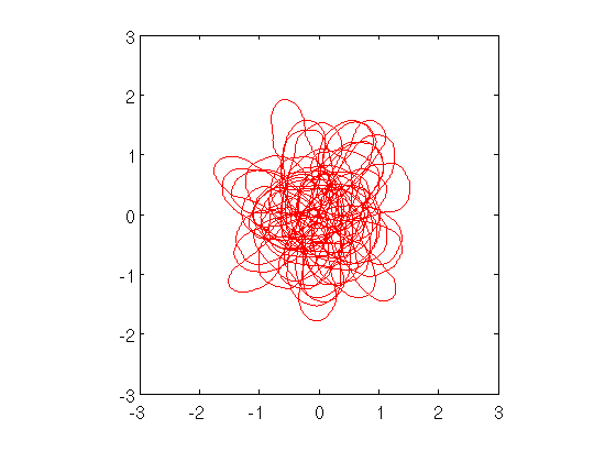
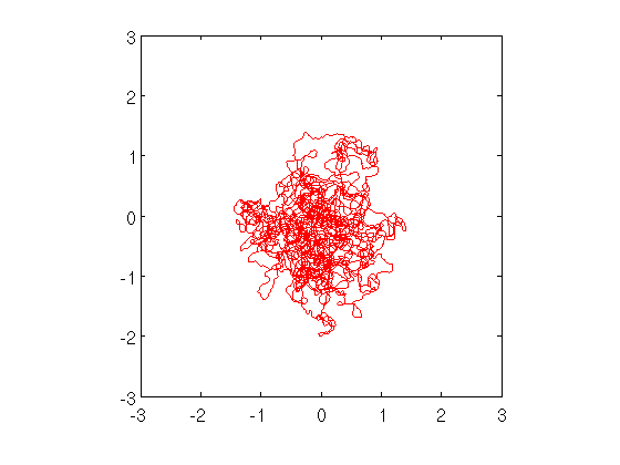
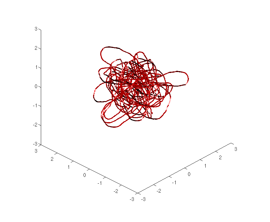
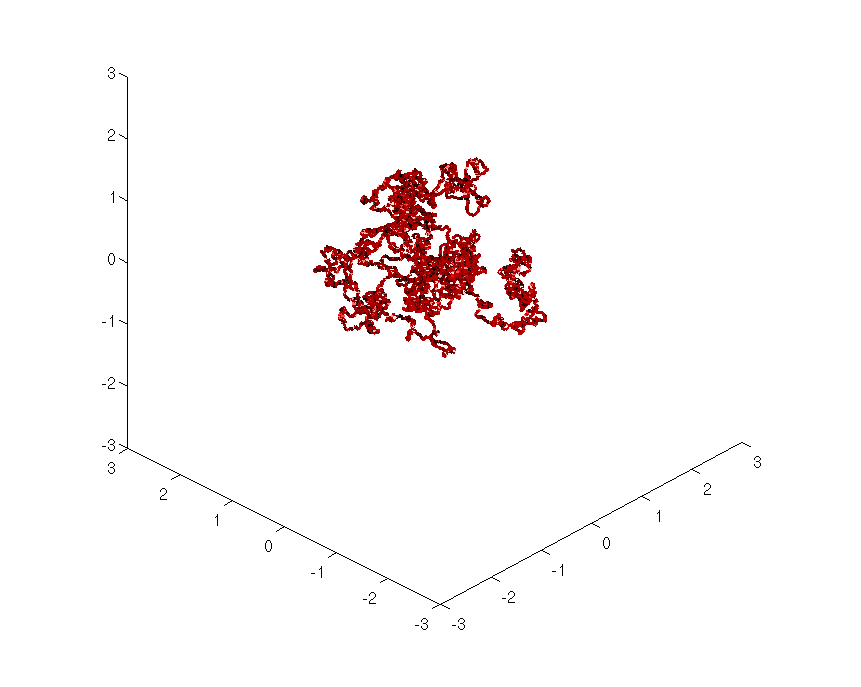
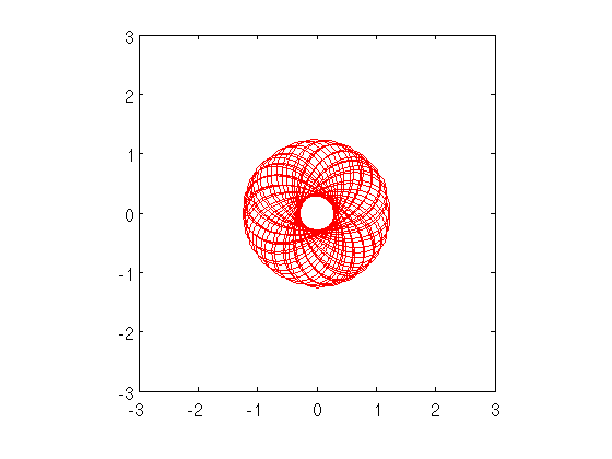
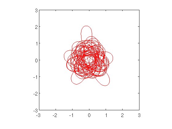
Figure 1. Two-dimensional case
Refer to caption
Refer to caption
Refer to caption
Refer to caption
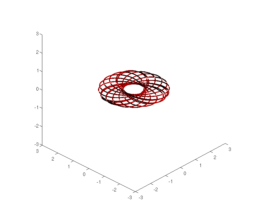
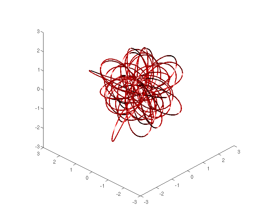
Figure 2. Three-dimensional case

3.6. Numerical simulations

For simulating our previously defined d𝑑d-dimensional fiber lay-down SDE (3.7), we may of course simulate SDE (3.9) directly in the underlying euclidean space 2dsuperscript2𝑑\mathbb{R}^{2d}. Nevertheless, this requires a consistent numerical algorithm staying on the manifold d×𝕊d1superscript𝑑superscript𝕊𝑑1\mathbb{R}^{d}\times\mathbb{S}^{d-1}.

Instead, we take another approach and rewrite our fiber lay-down SDE in local coordinate form. Therefore, let d𝑑d\in\mathbb{N}, d2𝑑2d\geq 2, and recall the following spherical coordinate system τd1(θ)=τd1(θ1,,θd1)subscript𝜏𝑑1𝜃subscript𝜏𝑑1subscript𝜃1subscript𝜃𝑑1\tau_{d-1}(\theta)=\tau_{d-1}(\theta_{1},\ldots,\theta_{d-1}) with θ1(0,2π)subscript𝜃102𝜋\theta_{1}\in(0,2\pi) and θj(0,π)subscript𝜃𝑗0𝜋\theta_{j}\in(0,\pi) for j=2,,d1𝑗2𝑑1j=2,\ldots,d-1, see the Appendix. Furthermore, note that τd1subscript𝜏𝑑1\tau_{d-1} is 2π2𝜋2\pi-periodic in θ1subscript𝜃1\theta_{1}. Consider the following SDE

dξ=τd1(θ)dtd𝜉subscript𝜏𝑑1𝜃dt\displaystyle\mathrm{d}\xi=\tau_{d-1}(\theta)\,\mathrm{dt} (3.11)
dθj=(𝒢j(θ)Φ(ξ)nj(θ)+σ22𝒢j2(θ)(j1)cot(θj))dt+σ𝒢j(θ)dWt(j)dsubscript𝜃𝑗subscript𝒢𝑗𝜃Φ𝜉subscript𝑛𝑗𝜃superscript𝜎22superscriptsubscript𝒢𝑗2𝜃𝑗1subscript𝜃𝑗dt𝜎subscript𝒢𝑗𝜃dsubscriptsuperscript𝑊𝑗𝑡\displaystyle\mathrm{d}\theta_{j}=\left(-\mathcal{G}_{j}(\theta)\,\nabla\Phi(\xi)\cdot n_{j}(\theta)+\frac{\sigma^{2}}{2}\,\mathcal{G}_{j}^{2}(\theta)\,(j-1)\cot(\theta_{j})\right)\,\mathrm{dt}+\sigma\,\mathcal{G}_{j}(\theta)\,\mathrm{d}W^{(j)}_{t}

with j=1,,d1𝑗1𝑑1j=1,\ldots,d-1. For abuse of notation, the time index t𝑡t is omitted. Here 𝒢jsubscript𝒢𝑗\mathcal{G}_{j} (with 𝒢d1:=1assignsubscript𝒢𝑑11\mathcal{G}_{d-1}:=1) and njsubscript𝑛𝑗n_{j} are given as

𝒢j(θ)=i=j+1d11sin(θi),nj(θ)=θjτd1(θ)|θjτd1(θ)|,j=1,,d1.formulae-sequencesubscript𝒢𝑗𝜃superscriptsubscriptproduct𝑖𝑗1𝑑11subscript𝜃𝑖formulae-sequencesubscript𝑛𝑗𝜃subscriptsubscript𝜃𝑗subscript𝜏𝑑1𝜃subscriptsubscript𝜃𝑗subscript𝜏𝑑1𝜃𝑗1𝑑1\displaystyle\mathcal{G}_{j}(\theta)=\prod_{i=j+1}^{d-1}\frac{1}{\sin(\theta_{i})},\leavevmode\nobreak\ n_{j}(\theta)=\frac{\partial_{\theta_{j}}\tau_{d-1}(\theta)}{|\partial_{\theta_{j}}\tau_{d-1}(\theta)|},\leavevmode\nobreak\ j=1,\ldots,d-1.

and W𝑊W denotes a standard (d1)𝑑1(d-1)-dimensional Brownian motion. Note that (3.11) writes as Stratonovich SDE in the same form. Let us justify this definition in the upcoming remark.

Remark 3.2.

SDE (3.11) should be understood analogously as in Section 3.2 as some manifold-valued Stratonovich SDE with state space d×𝕋×(0,π)d2superscript𝑑𝕋superscript0𝜋𝑑2\mathbb{R}^{d}\times\mathbb{T}\times(0,\pi)^{d-2}, or state space 2×𝕋superscript2𝕋\mathbb{R}^{2}\times\mathbb{T} in case d=2𝑑2d=2, respectively. By using Formulas (7.27) and (7.28) from the Appendix, observe that the generator corresponding to (3.11) coincides with the fiber lay-down generator L𝐿L computed on d×𝕋×(0,π)d2superscript𝑑𝕋superscript0𝜋𝑑2\mathbb{R}^{d}\times\mathbb{T}\times(0,\pi)^{d-2}. Now assume that there exists a solution Y𝑌Y to (3.11) starting from (ξ,θ1,,θd1)𝜉subscript𝜃1subscript𝜃𝑑1(\xi,\theta_{1},\ldots,\theta_{d-1}) and having infinite lifetime. Then it is easy to see that X𝑋X, defined by Xt:=(ξ(t),τd1(θ1(t),,θd1(t)))assignsubscript𝑋𝑡𝜉𝑡subscript𝜏𝑑1subscript𝜃1𝑡subscript𝜃𝑑1𝑡X_{t}:=\left(\xi(t),\tau_{d-1}(\theta_{1}(t),\ldots,\theta_{d-1}(t))\right), is a L𝐿L-diffusion. Hence X𝑋X coincides weakly with any solution of the d𝑑d-dimensional fiber lay-down SDE (3.7) starting from (ξ,τd1(θ1,,θd1))𝜉subscript𝜏𝑑1subscript𝜃1subscript𝜃𝑑1(\xi,\tau_{d-1}(\theta_{1},\ldots,\theta_{d-1})).

Summarizing, the simulation of SDE (3.11) gives us a (local) L𝐿L-diffusion, L𝐿L being our d𝑑d-dimensional fiber lay down generator. Thus it is reasonable to call (3.11) simply the d𝑑d-dimensional fiber lay down SDE in local coordinate form. Note that in case d=2𝑑2d=2, (3.11) reduces to (1.1) (or (3.4) respectively) and in case d=3𝑑3d=3 we obtain back the three-dimensional fiber lay down model derived in [KMW12]. In Figure 1 and Figure 2, let us illustrate and compare the ξ𝜉\xi-trajectories in case d=2𝑑2d=2, d=3𝑑3d=3, for different values of σ𝜎\sigma where σ=0, 0.1, 0.5, 4.0𝜎00.10.54.0\sigma=0,\leavevmode\nobreak\ 0.1,\leavevmode\nobreak\ 0.5,\leavevmode\nobreak\ 4.0. ΦΦ\Phi is chosen as Φ=|ξ|2Φsuperscript𝜉2\Phi=|\xi|^{2}.

4. Global solutions to the stochastic equations

Before studying the long time behaviour of solutions to our d𝑑d-dimensional fiber lay-down equations, we shall discuss basic existence statements of the underlying stochastic equations itself.

4.1. The two-dimensional model

First we analyze the basic two-dimensional model, i.e., the Itô SDE (1.1) in 3superscript3\mathbb{R}^{3}. Φ(ξ)=aξ12+bξ22Φ𝜉𝑎superscriptsubscript𝜉12𝑏superscriptsubscript𝜉22\Phi(\xi)=a\,\xi_{1}^{2}+b\,\xi_{2}^{2}, a,b𝑎𝑏a,b\in\mathbb{R}, a,b0𝑎𝑏0a,b\geq 0, treats the physical relevant situation, see [KMW09]. It is easy to verify that in this case the drift vector of the underlying SDE is not globally Lipschitz continuous and one may ask under which conditions the stochastic equation admits a global solution. Therefore, we rewrite the equation in a bit more general form as

dξt=τ(αt)dtdsubscript𝜉𝑡𝜏subscript𝛼𝑡dt\displaystyle\mathrm{d}\xi_{t}=\tau(\alpha_{t})\,\mathrm{dt} (4.12)
dαt=Ψ(ξt)τ(αt)dt+σdWt.dsubscript𝛼𝑡Ψsubscript𝜉𝑡superscript𝜏bottomsubscript𝛼𝑡dt𝜎dsubscript𝑊𝑡\displaystyle\mathrm{d}\alpha_{t}=\Psi(\xi_{t})\cdot\tau^{\bot}(\alpha_{t})\,\mathrm{dt}+\sigma\,\mathrm{d}W_{t}.

The following proposition shows that even under the assumption of ΨΨ\Psi being locally Lipschitz, explosion is not possible and SDE (4.12) admits a classical globally defined strong solution.

Proposition 4.1.

Let Ψ:22:Ψsuperscript2superscript2\Psi:\mathbb{R}^{2}\rightarrow\mathbb{R}^{2} be locally Lipschitz continuous. Given a filtered probability space (Ω,,,{t}t0)Ωsubscriptsubscript𝑡𝑡0(\Omega,\mathcal{F},\mathbb{P},\{\mathcal{F}_{t}\}_{t\geq 0}) together with an one-dimensional {t}t0subscriptsubscript𝑡𝑡0\{\mathcal{F}_{t}\}_{t\geq 0}-Brownian motion W={Wt}t0𝑊subscriptsubscript𝑊𝑡𝑡0W=\{W_{t}\}_{t\geq 0}. Then for each 0subscript0\mathcal{F}_{0}-measurable x0:Ω3:subscript𝑥0Ωsuperscript3x_{0}:\Omega\rightarrow\mathbb{R}^{3} there exists a unique {t}t0subscriptsubscript𝑡𝑡0\{\mathcal{F}_{t}\}_{t\geq 0}-adapted continuous 3superscript3\mathbb{R}^{3}-valued process X={Xt}t0𝑋subscriptsubscript𝑋𝑡𝑡0X=\{X_{t}\}_{t\geq 0} which satisfies X0=x0subscript𝑋0subscript𝑥0X_{0}=x_{0} \mathbb{P}-a.s. and solves (4.12) in integral form.

Proof.

The classical Picard-Lindel"of iteration scheme can be applied pathwise for each ωΩ𝜔Ω\omega\in\Omega. This is due to the special structure of our equation. We follow the strategy from [KS91, Ch. 5; Ex. 2.19]. So let t0𝑡0t\geq 0, n0={0}𝑛subscript00n\in\mathbb{N}_{0}=\mathbb{N}\cup\{0\}, and define

Xt(0):=x0,Xt(n+1):=x0+0tb(Xs(n))ds+AWtformulae-sequenceassignsubscriptsuperscript𝑋0𝑡subscript𝑥0assignsubscriptsuperscript𝑋𝑛1𝑡subscript𝑥0superscriptsubscript0𝑡𝑏subscriptsuperscript𝑋𝑛𝑠differential-d𝑠𝐴subscript𝑊𝑡\displaystyle X^{(0)}_{t}:=x_{0},\leavevmode\nobreak\ X^{(n+1)}_{t}:=x_{0}+\int_{0}^{t}{b(X^{(n)}_{s})}\,\mathrm{d}s+A\,W_{t}

where b(ξ,α):=(τ(α),Ψ(ξ)τ(α))T,A:=(0,0,σ)Tformulae-sequenceassign𝑏𝜉𝛼superscript𝜏𝛼Ψ𝜉superscript𝜏bottom𝛼𝑇assign𝐴superscript00𝜎𝑇b(\xi,\alpha):=(\tau(\alpha),\Psi(\xi)\cdot\tau^{\bot}(\alpha))^{T},\leavevmode\nobreak\ A:=\left(0,0,\sigma\right)^{T}. Then X(n)={Xt(n)}t0superscript𝑋𝑛subscriptsubscriptsuperscript𝑋𝑛𝑡𝑡0X^{(n)}=\{X^{(n)}_{t}\}_{t\geq 0}, n0𝑛subscript0n\in\mathbb{N}_{0}, is easily seen to be continuous and {t}t0subscriptsubscript𝑡𝑡0\{\mathcal{F}_{t}\}_{t\geq 0}-adapted.
Now fix T>0𝑇0T>0 and ωΩ𝜔Ω\omega\in\Omega. Observe that the first two components of Xt(n)(ω)subscriptsuperscript𝑋𝑛𝑡𝜔X^{(n)}_{t}(\omega) are bounded by N:=|x0(ω)|+Tassign𝑁subscript𝑥0𝜔𝑇N:=\left|x_{0}(\omega)\right|+T for each n0𝑛subscript0n\in\mathbb{N}_{0}, t[0,T]𝑡0𝑇t\in[0,T]. Now N𝑁N only depends on ω𝜔\omega and T𝑇T. Thus we may restrict b𝑏b to [N,N] 2×superscript𝑁𝑁2[-N,N]^{\,2}\times\mathbb{R} in the definition of Xt(n)(ω)subscriptsuperscript𝑋𝑛𝑡𝜔X^{(n)}_{t}(\omega) for all n0𝑛subscript0n\in\mathbb{N}_{0}, t[0,T]𝑡0𝑇t\in[0,T]. Furthermore, observe that b𝑏b is Lipschitz continuous on each K×𝐾K\times\mathbb{R}, K2𝐾superscript2K\subseteq\mathbb{R}^{2} compact. In particular, there exists some constant L𝐿L, depending on ω𝜔\omega and T𝑇T, such that |b(x)b(y)|L|xy|𝑏𝑥𝑏𝑦𝐿𝑥𝑦\left|b(x)-b(y)\right|\leq L\left|x-y\right| for all x,y[N,N] 2×𝑥𝑦superscript𝑁𝑁2x,y\in[-N,N]^{\,2}\times\mathbb{R}. So altogether

|b(Xt(n)(ω))b(Xt(n1)(ω))|L|Xt(n)(ω)Xt(n1)(ω)|𝑏subscriptsuperscript𝑋𝑛𝑡𝜔𝑏subscriptsuperscript𝑋𝑛1𝑡𝜔𝐿subscriptsuperscript𝑋𝑛𝑡𝜔subscriptsuperscript𝑋𝑛1𝑡𝜔\displaystyle\left|b(X^{(n)}_{t}(\omega))-b(X^{(n-1)}_{t}(\omega))\right|\leq L\,\left|X^{(n)}_{t}(\omega)-X^{(n-1)}_{t}(\omega)\right| (4.13)

holds for all n,t[0,T]formulae-sequence𝑛𝑡0𝑇n\in\mathbb{N},\leavevmode\nobreak\ t\in[0,T]. Now we may continue as in the classical case. Indeed, for those n𝑛n and t𝑡t we define

Dt(n)(ω)=max0st|Xs(n)(ω)Xs(n1)(ω)|.subscriptsuperscript𝐷𝑛𝑡𝜔subscript0𝑠𝑡subscriptsuperscript𝑋𝑛𝑠𝜔subscriptsuperscript𝑋𝑛1𝑠𝜔\displaystyle D^{(n)}_{t}(\omega)=\max_{0\leq s\leq t}\left|X^{(n)}_{s}(\omega)-X^{(n-1)}_{s}(\omega)\right|.

Then (4.13) yields Dt(n)(ω)L0tDs(n1)(ω)dssubscriptsuperscript𝐷𝑛𝑡𝜔𝐿superscriptsubscript0𝑡subscriptsuperscript𝐷𝑛1superscript𝑠𝜔differential-dsuperscript𝑠D^{(n)}_{t}(\omega)\leq L\int_{0}^{t}{D^{(n-1)}_{s^{\prime}}(\omega)\,\mathrm{d}s^{\prime}} for n2𝑛2n\geq 2 and t[0,T]𝑡0𝑇t\in[0,T]. Moreover, Dt(1)(ω)subscriptsuperscript𝐷1𝑡𝜔D^{(1)}_{t}(\omega) is bounded for t[0,T]𝑡0𝑇t\in[0,T] by K:=T|b(x0(ω))|+σmax0sT|Ws(ω)|assign𝐾𝑇𝑏subscript𝑥0𝜔𝜎subscript0𝑠𝑇subscript𝑊𝑠𝜔K:=T\,|b(x_{0}(\omega))|+\sigma\,\max_{0\leq s\leq T}\left|W_{s}(\omega)\right| which also depends only on ω𝜔\omega and T𝑇T. Thus inductively we get

Dt(n)(ω)K(Lt)n1(n1)!,n,t[0,T].formulae-sequencesubscriptsuperscript𝐷𝑛𝑡𝜔𝐾superscript𝐿𝑡𝑛1𝑛1formulae-sequence𝑛𝑡0𝑇\displaystyle D^{(n)}_{t}(\omega)\leq K\,\frac{(L\,t)^{n-1}}{(n-1)!},\leavevmode\nobreak\ n\in\mathbb{N},\leavevmode\nobreak\ t\in[0,T].

Now let n>m𝑛𝑚n>m, t[0,T]𝑡0𝑇t\in[0,T]. The latter estimate implies

max0st|Xs(n)(ω)Xs(m)(ω)|subscript0𝑠𝑡subscriptsuperscript𝑋𝑛𝑠𝜔subscriptsuperscript𝑋𝑚𝑠𝜔\displaystyle\max_{0\leq s\leq t}\left|X^{(n)}_{s}(\omega)-X^{(m)}_{s}(\omega)\right| j=mn1max0st|Xs(j+1)(ω)Xs(j)(ω)|Kj=m(Lt)jj!.absentsuperscriptsubscript𝑗𝑚𝑛1subscript0𝑠𝑡subscriptsuperscript𝑋𝑗1𝑠𝜔subscriptsuperscript𝑋𝑗𝑠𝜔𝐾superscriptsubscript𝑗𝑚superscript𝐿𝑡𝑗𝑗\displaystyle\leq\sum_{j=m}^{n-1}{\max_{0\leq s\leq t}\left|X^{(j+1)}_{s}(\omega)-X^{(j)}_{s}(\omega)\right|}\leq K\sum_{j=m}^{\infty}{\frac{(L\,t)^{j}}{j!}}.

Hence X(n)(ω)superscript𝑋𝑛𝜔X^{(n)}(\omega), n𝑛n\in\mathbb{N}, converges uniformly on [0,T]0𝑇[0,T] to some continuous function Xt(ω)subscript𝑋𝑡𝜔X_{t}(\omega) where 0tT0𝑡𝑇0\leq t\leq T. Further note that Xt(ω)subscript𝑋𝑡𝜔X_{t}(\omega) is contained in [N,N] 2×superscript𝑁𝑁2[-N,N]^{\,2}\times\mathbb{R} for all t[0,T]𝑡0𝑇t\in[0,T], since Xt(n)(ω)subscriptsuperscript𝑋𝑛𝑡𝜔X^{(n)}_{t}(\omega) satisfies this property independent of n𝑛n\in\mathbb{N}. Hence for t[0,T]𝑡0𝑇t\in[0,T] we conclude

|0tb(Xs(n)(ω))ds0tb(Xs(ω))ds|tLmax0st|Xs(n)(ω)Xs(ω)|n0.superscriptsubscript0𝑡𝑏subscriptsuperscript𝑋𝑛𝑠𝜔differential-d𝑠superscriptsubscript0𝑡𝑏subscript𝑋𝑠𝜔differential-d𝑠𝑡𝐿subscript0𝑠𝑡subscriptsuperscript𝑋𝑛𝑠𝜔subscript𝑋𝑠𝜔superscript𝑛0\displaystyle\left|\int_{0}^{t}{b(X^{(n)}_{s}(\omega))\,\mathrm{d}s}-\int_{0}^{t}{b(X_{s}(\omega))\,\mathrm{d}s}\right|\leq t\,L\,\max_{0\leq s\leq t}\left|X^{(n)}_{s}(\omega)-X_{s}(\omega)\right|\stackrel{{\scriptstyle n\rightarrow\infty}}{{\longrightarrow}}0.

This shows that Xt(ω)subscript𝑋𝑡𝜔X_{t}(\omega), 0tT0𝑡𝑇0\leq t\leq T, solves (4.12) in integral form. Now the previous construction holds for all T0𝑇0T\geq 0 and each ωΩ𝜔Ω\omega\in\Omega, hence the map tXt(ω)maps-to𝑡subscript𝑋𝑡𝜔t\mapsto X_{t}(\omega), t0𝑡0t\geq 0, is well-defined and continuous. Clearly, Xtsubscript𝑋𝑡X_{t} is tsubscript𝑡\mathcal{F}_{t}-measurable, t0𝑡0t\geq 0. Concerning the uniqueness statement, see e.g. [KS91, Ch. 5, Theo. 2.5]. ∎

Now we are able to solve easily the two-dimensional fiber lay-down SDE (3.4) with state space 2×𝕋superscript2𝕋\mathbb{R}^{2}\times\mathbb{T} without using any abstract arguments. For simplicity we shall assume ΦC(2)Φsuperscript𝐶superscript2\Phi\in C^{\infty}(\mathbb{R}^{2}) to stay consistent with the (smooth) manifold language. Concerning all the following uniqueness statements, we refer to [Hsu02, Prop. 1.2.9].

Corollary 4.2.

Let ΦC(2)Φsuperscript𝐶superscript2\Phi\in C^{\infty}(\mathbb{R}^{2}). Then there exists a unique solution X={Xt}t0𝑋subscriptsubscript𝑋𝑡𝑡0X=\{X_{t}\}_{t\geq 0} with infinite lifetime of the two-dimensional fiber lay-down SDE(𝒜0,𝒜1;W,x0)SDEsubscript𝒜0subscript𝒜1𝑊subscript𝑥0\text{SDE}(\mathcal{A}_{0},\mathcal{A}_{1};W,x_{0}), see Equation (3.4), with state space 2×𝕋superscript2𝕋\mathbb{R}^{2}\times\mathbb{T}.

Proof.

Consider the canonical projection P:32×𝕋:Psuperscript3superscript2𝕋\mathrm{P}:\mathbb{R}^{3}\rightarrow\mathbb{R}^{2}\times\mathbb{T}. Now we may choose some x~0:Ω3:subscript~𝑥0Ωsuperscript3\widetilde{x}_{0}:\Omega\rightarrow\mathbb{R}^{3} being 0subscript0\mathcal{F}_{0}-measurable that satisfies x0=Px~0subscript𝑥0Psubscript~𝑥0x_{0}=\mathrm{P}\circ\widetilde{x}_{0}. Such an x~0subscript~𝑥0\widetilde{x}_{0} exists since the map φ:[0,2π)𝕋,x[x]:𝜑formulae-sequence02𝜋𝕋maps-to𝑥delimited-[]𝑥\varphi:[0,2\pi)\rightarrow\mathbb{T},x\mapsto[x], is a Borel isomorphism, see [Par67, Cor. I.3.3]. Proposition 4.1 (with Ψ=ΦΨΦ\Psi=-\nabla\Phi) is applicable and yields the existence of a strong solution X~~𝑋\widetilde{X} to SDE (4.12) with initial condition x~0subscript~𝑥0\widetilde{x}_{0} relative to (Ω,,,{t}t0,W)Ωsubscriptsubscript𝑡𝑡0𝑊(\Omega,\mathcal{F},\mathbb{P},\{\mathcal{F}_{t}\}_{t\geq 0},W). The process X𝑋X, defined by Xt=PX~tsubscript𝑋𝑡Psubscript~𝑋𝑡X_{t}=\mathrm{P}\circ\widetilde{X}_{t}, t0𝑡0t\geq 0, satisfies X0=x0subscript𝑋0subscript𝑥0X_{0}=x_{0} \mathbb{P}-a.s. and has infinite lifetime. The fact that X𝑋X solves SDE(𝒜0,𝒜1;W,x0)SDEsubscript𝒜0subscript𝒜1𝑊subscript𝑥0\text{SDE}(\mathcal{A}_{0},\mathcal{A}_{1};W,x_{0}) has already been verified in Section 3.2. ∎

4.2. The d𝑑d-dimensional fiber lay-down model

The same statement as before remains true for our general d𝑑d-dimensional equation.

Proposition 4.3.

Let ΦC(d)Φsuperscript𝐶superscript𝑑\Phi\in C^{\infty}(\mathbb{R}^{d}), d2𝑑2d\geq 2. Then there exists a unique solution X𝑋X with infinite lifetime to the d𝑑d-dimensional fiber lay-down SDE(𝒩0,,𝒩n;W,x0)SDEsubscript𝒩0subscript𝒩𝑛𝑊subscript𝑥0\text{SDE}(\mathcal{N}_{0},\ldots,\mathcal{N}_{n};W,x_{0}), see Equation (3.7), with state space d×𝕊d1superscript𝑑superscript𝕊𝑑1\mathbb{R}^{d}\times\mathbb{S}^{d-1}.

Proof.

By [Hsu02, Theo. 1.2.9] we know that there exists a unique continuous solution X𝑋X to SDE(𝒩0,,𝒩n;W,x0)SDEsubscript𝒩0subscript𝒩𝑛𝑊subscript𝑥0\text{SDE}(\mathcal{N}_{0},\ldots,\mathcal{N}_{n};W,x_{0}) with state space d×𝕊d1superscript𝑑superscript𝕊𝑑1\mathbb{R}^{d}\times\mathbb{S}^{d-1} up to its lifetime e𝑒e. It remains to check that e(X)=𝑒𝑋e(X)=\infty holds \mathbb{P}-almost surely. Write Xt=(ξt,vt)subscript𝑋𝑡subscript𝜉𝑡subscript𝑣𝑡X_{t}=(\xi_{t},v_{t}), t<e(X)𝑡𝑒𝑋t<e(X). For each fCc(d)𝑓superscriptsubscript𝐶𝑐superscript𝑑f\in C_{c}^{\infty}(\mathbb{R}^{d}) we have

f(ξt)f(ξ0)=0tvsξf(ξs)ds, 0t<e(X).formulae-sequence𝑓subscript𝜉𝑡𝑓subscript𝜉0superscriptsubscript0𝑡subscript𝑣𝑠subscript𝜉𝑓subscript𝜉𝑠differential-d𝑠 0𝑡𝑒𝑋\displaystyle f(\xi_{t})-f(\xi_{0})=\int_{0}^{t}v_{s}\cdot\nabla_{\xi}f(\xi_{s})\,\mathrm{d}s,\leavevmode\nobreak\ 0\leq t<e(X).

In particular, this identity holds for all fCc(d)𝑓superscriptsubscript𝐶𝑐superscript𝑑f\in C_{c}^{\infty}(\mathbb{R}^{d}) which satisfy f(ξ)=ξj𝑓𝜉subscript𝜉𝑗f(\xi)=\xi_{j} for j=1,,d𝑗1𝑑j=1,\ldots,d, inside some balls Br(0)subscript𝐵𝑟0B_{r}(0) of radius r>0𝑟0r>0 large enough. Then we easily conclude

ξtξ0=0tvsds, 0t<e(X).formulae-sequencesubscript𝜉𝑡subscript𝜉0superscriptsubscript0𝑡subscript𝑣𝑠differential-d𝑠 0𝑡𝑒𝑋\displaystyle\xi_{t}-\xi_{0}=\int_{0}^{t}v_{s}\,\mathrm{d}s,\leavevmode\nobreak\ 0\leq t<e(X). (4.14)

Consequently, |ξtξ0|tsubscript𝜉𝑡subscript𝜉0𝑡\left|\xi_{t}-\xi_{0}\right|\leq t for 0t<e(X)0𝑡𝑒𝑋0\leq t<e(X). Now assume that e(X)<𝑒𝑋e(X)<\infty holds on some A𝐴A\in\mathcal{F} with (A)>0𝐴0\mathbb{P}(A)>0. But then |Xt|2nsubscriptsubscript𝑋𝑡superscript2𝑛\left|X_{t}\right|_{\mathbb{R}^{2n}}\rightarrow\infty and hence |ξt|subscript𝜉𝑡\left|\xi_{t}\right|\rightarrow\infty as te(X)𝑡𝑒𝑋t\uparrow e(X) on A𝐴A, see e.g. [Hsu02, Prop. 1.2.6]. But this contradicts the previous inequality. ∎

5. Convergence to equilibrium: Mixing properties

As mentioned in the introduction, we start in this section with the investigating of the long time behaviour of our d𝑑d-dimensional fiber lay-down process by proving strong mixing properties. We make use of a new version of Doob’s theorem derived recently in [GN12]. But first we introduce some notations that are used until the end of this article.

5.1. Motivation and setup.

In the following let d𝑑d\in\mathbb{N}, d2𝑑2d\geq 2. We focus attention on the d𝑑d-dimensional fiber lay-down SDE with state space 𝕄:=d×𝕊d1assign𝕄superscript𝑑superscript𝕊𝑑1\mathbb{M}:=\mathbb{R}^{d}\times\mathbb{S}^{d-1}

dXt=𝒩0(Xt)dt+j=1d𝒩j(Xt)dWt(j)dsubscript𝑋𝑡subscript𝒩0subscript𝑋𝑡dtsuperscriptsubscript𝑗1𝑑subscript𝒩𝑗subscript𝑋𝑡dsubscriptsuperscript𝑊𝑗𝑡\displaystyle\mathrm{d}X_{t}=\mathcal{N}_{0}(X_{t})\,\mathrm{dt}+\sum_{j=1}^{d}\mathcal{N}_{j}(X_{t})\circ\mathrm{d}W^{(j)}_{t} (5.15)

where W𝑊W is a standard d𝑑d-dimensional Brownian motion. For computational convenience, we replace ΦΦ\Phi by 1d1Φ1𝑑1Φ\frac{1}{d-1}\Phi in SDE (5.15). So 𝒩0subscript𝒩0\mathcal{N}_{0} is redefined as

𝒩0(ξ,v):=(v1d1(Ivv)Φ(ξ)),(ξ,v)d×𝕊d1.formulae-sequenceassignsubscript𝒩0𝜉𝑣matrix𝑣1𝑑1𝐼tensor-product𝑣𝑣Φ𝜉𝜉𝑣superscript𝑑superscript𝕊𝑑1\displaystyle\mathcal{N}_{0}(\xi,v):=\begin{pmatrix}v\\ -\frac{1}{d-1}(I-v\otimes v)\nabla\Phi(\xi)\end{pmatrix},(\xi,v)\in\mathbb{R}^{d}\times\mathbb{S}^{d-1}.

The vector fields 𝒩jsubscript𝒩𝑗\mathcal{N}_{j} are defined in (3.8). Convention: The first d𝑑d-components of 2dsuperscript2𝑑\mathbb{R}^{2d} are abbreviated by ξ𝜉\xi whereas the last d𝑑d-variables are denoted by v𝑣v. We consider potentials Φ:d:Φsuperscript𝑑\Phi:\mathbb{R}^{d}\rightarrow\mathbb{R} such that eΦL1(d,dξ)superscript𝑒Φsuperscript𝐿1superscript𝑑d𝜉e^{-\Phi}\in L^{1}(\mathbb{R}^{d},\mathrm{d}\xi). Thus without loss of generality we assume in the following

deΦdξ=1.subscriptsuperscript𝑑superscript𝑒Φdifferential-d𝜉1\displaystyle\int_{\mathbb{R}^{d}}e^{-\Phi}\,\mathrm{d}\xi=1.

We introduce the probability measure μ𝜇\mu on (𝕄,(𝕄))𝕄𝕄(\mathbb{M},\mathcal{B}(\mathbb{M})) defined by

μ:=eΦdξν,ν:=1vol(𝕊d1)𝒮.formulae-sequenceassign𝜇tensor-productsuperscript𝑒Φ𝑑𝜉𝜈assign𝜈1volsuperscript𝕊𝑑1𝒮\displaystyle\mu:=e^{-\Phi}d\xi\otimes\nu,\leavevmode\nobreak\ \nu:=\frac{1}{\text{vol}(\mathbb{S}^{d-1})}\,\mathcal{S}.

Here 𝒮𝒮\mathcal{S} denotes the surface measure of 𝕊d1superscript𝕊𝑑1\mathbb{S}^{d-1}, vol(𝕊d1)volsuperscript𝕊𝑑1\text{vol}(\mathbb{S}^{d-1}) the surface area of 𝕊d1superscript𝕊𝑑1\mathbb{S}^{d-1} and (𝕄)𝕄\mathcal{B}(\mathbb{M}) the Borel-sigma-algebra on 𝕄𝕄\mathbb{M}. The Kolmogorov operator L=vξgrad𝕊d1V+σ22Δ𝕊d1𝐿𝑣subscript𝜉subscriptgradsuperscript𝕊𝑑1𝑉superscript𝜎22subscriptΔsuperscript𝕊𝑑1L=v\cdot\nabla_{\xi}-\text{grad}_{\mathbb{S}^{d-1}}V+\frac{\sigma^{2}}{2}\,\Delta_{\mathbb{S}^{d-1}}, see (3.10), associated to SDE (3.7) is also sometimes denoted by LKsuperscript𝐿KL^{\text{K}} where V:𝕄:𝑉𝕄V:\mathbb{M}\rightarrow\mathbb{R} is now given as V(ξ,v)=1d1Φ(ξ)v𝑉𝜉𝑣1𝑑1Φ𝜉𝑣V(\xi,v)=\frac{1}{d-1}\,\nabla\Phi(\xi)\cdot v.

Moreover, we denote by Xx={Xtx}t0superscript𝑋𝑥subscriptsubscriptsuperscript𝑋𝑥𝑡𝑡0X^{x}=\{X^{x}_{t}\}_{t\geq 0} the solution to SDE (5.15) with initial value x𝕄𝑥𝕄x\in\mathbb{M}. Formally, its corresponding probability density ftsubscript𝑓𝑡f_{t} (with respect to dξ𝒮tensor-productd𝜉𝒮\mathrm{d}\xi\otimes\mathcal{S} and Dirac initial state x𝑥x) satisfies the Fokker-Planck equation tf=LFPfsubscript𝑡𝑓superscript𝐿FP𝑓\partial_{t}f=L^{\text{FP}}f with LFPsuperscript𝐿FPL^{\text{FP}} being the Fokker-Planck operator associated to the d𝑑d-dimensional fiber lay-down model. The latter is given as the (algebraic) adjoint of LKsuperscript𝐿KL^{\text{K}} in L2(𝕄,dξ𝒮)superscript𝐿2𝕄tensor-productd𝜉𝒮L^{2}(\mathbb{M},\mathrm{d}\xi\otimes\mathcal{S}). Thus, using Lemma 7.2 from the Appendix below, we get

LFP=vξ+grad𝕊d1VΦ(ξ)v+σ22ΔSd1.superscript𝐿FP𝑣subscript𝜉subscriptgradsuperscript𝕊𝑑1𝑉Φ𝜉𝑣superscript𝜎22subscriptΔsuperscriptS𝑑1\displaystyle L^{\text{FP}}=-v\cdot\nabla_{\xi}+\text{grad}_{\mathbb{S}^{d-1}}V-\nabla\Phi(\xi)\cdot v+\frac{\sigma^{2}}{2}\,\,\Delta_{\mathrm{S}^{d-1}}.

So, up to normalization, a stationary solution to the Fokker-Planck equation is now given by

(ξ,v)F(ξ,v):=eΦ(ξ),(ξ,v)𝕄.formulae-sequencemaps-to𝜉𝑣𝐹𝜉𝑣assignsuperscript𝑒Φ𝜉𝜉𝑣𝕄\displaystyle(\xi,v)\mapsto F(\xi,v):=e^{-\Phi(\xi)},\leavevmode\nobreak\ (\xi,v)\in\mathbb{M}.

Hence we expect that ftsubscript𝑓𝑡f_{t} converges towards 1vol(𝕊d1)F1volsuperscript𝕊𝑑1𝐹\frac{1}{\text{vol}(\mathbb{S}^{d-1})}\,F as t𝑡t\rightarrow\infty. In other words, Xtxsuperscriptsubscript𝑋𝑡𝑥X_{t}^{x} should be distributed accordingly to μ𝜇\mu for large values of t0𝑡0t\geq 0. Now formally, u(t,x)=𝔼[u0(Xtx)]𝑢𝑡𝑥𝔼delimited-[]subscript𝑢0subscriptsuperscript𝑋𝑥𝑡u(t,x)=\mathbb{E}[u_{0}(X^{x}_{t})] solves the Kolmogorov PDE tu=Lusubscript𝑡𝑢𝐿𝑢\partial_{t}u=Lu with initial state u(t=0)=u0𝑢𝑡0subscript𝑢0u(t=0)=u_{0}. Hence altogether the subsequent analysis in the previous and the upcoming section has the interpretation of proving convergence of 𝔼[u0(Xtx)]𝔼delimited-[]subscript𝑢0subscriptsuperscript𝑋𝑥𝑡\mathbb{E}[u_{0}(X^{x}_{t})] towards 𝔼[u0(Xx)]:=𝕄u0dμassign𝔼delimited-[]subscript𝑢0subscriptsuperscript𝑋𝑥subscript𝕄subscript𝑢0differential-d𝜇\mathbb{E}[u_{0}(X^{x}_{\infty})]:=\int_{\mathbb{M}}u_{0}\,\mathrm{d}\mu. We now start with the mentioned strong mixing properties.

5.2. Mixing properties

First, we need the following lemma. Therefore, for given vector fields 𝒱1,,𝒱r,subscript𝒱1subscript𝒱𝑟\mathcal{V}_{1},\ldots,\mathcal{V}_{r}, on some manifold 𝕏𝕏\mathbb{X} we denote the least \mathbb{R}-vector space including all 𝒱jsubscript𝒱𝑗\mathcal{V}_{j}, j=1,,r,𝑗1𝑟j=1,\ldots,r, which is closed under the Lie-bracket operation by L(𝒱1,,𝒱r)𝐿subscript𝒱1subscript𝒱𝑟L(\mathcal{V}_{1},\ldots,\mathcal{V}_{r}).

Lemma 5.1.

For the vector fields 𝒩jsubscript𝒩𝑗\mathcal{N}_{j}, j=0,1,,d,𝑗01𝑑j=0,1,\ldots,d, from (3.8) it holds

dimL(𝒩1,,𝒩d,𝒩0+t)=2d at each point of (0,)×𝕄dim𝐿subscript𝒩1subscript𝒩𝑑subscript𝒩0𝑡2𝑑 at each point of (0,)×𝕄\displaystyle\mbox{dim}\leavevmode\nobreak\ L\big{(}\mathcal{N}_{1},\ldots,\mathcal{N}_{d},\mathcal{N}_{0}+\frac{\partial}{\partial t}\big{)}=2d\mbox{ at each point of $(0,\infty)\times\mathbb{M}$}

where we assume σ>0𝜎0\sigma>0.

Proof.

We may set σ=1𝜎1\sigma=1 and choose p=(t,ξ,v)(0,)×𝕄𝑝𝑡𝜉𝑣0𝕄p=(t,\xi,v)\in(0,\infty)\times\mathbb{M} arbitrary. First note that

span{v}span{(Ivv)ej|j=1,,d}=span{v}Tv𝕊d1=d.direct-sumspan𝑣spanconditional-set𝐼tensor-product𝑣𝑣subscript𝑒𝑗𝑗1𝑑direct-sumspan𝑣subscript𝑇𝑣superscript𝕊𝑑1superscript𝑑\displaystyle\text{span}\{v\}\oplus\text{span}\{(I-v\otimes v)e_{j}\leavevmode\nobreak\ |\leavevmode\nobreak\ j=1,\ldots,d\}=\text{span}\{v\}\oplus T_{v}\mathbb{S}^{d-1}=\mathbb{R}^{d}.

Observe that [𝒩j,𝒩0+t]subscript𝒩𝑗subscript𝒩0𝑡\left[\mathcal{N}_{j},\mathcal{N}_{0}+\frac{\partial}{\partial t}\right] for j=1,,d,𝑗1𝑑j=1,\ldots,d, is of the form

𝒜j:=[𝒩j,𝒩0+t]=(Ivv)ejξ+f1(j)(ξ,v)vassignsubscript𝒜𝑗subscript𝒩𝑗subscript𝒩0𝑡𝐼tensor-product𝑣𝑣subscript𝑒𝑗subscript𝜉superscriptsubscript𝑓1𝑗𝜉𝑣subscript𝑣\displaystyle\mathcal{A}_{j}:=\left[\mathcal{N}_{j},\mathcal{N}_{0}+\frac{\partial}{\partial t}\right]=(I-v\otimes v)e_{j}\cdot\nabla_{\xi}+f_{1}^{\,(j)}(\xi,v)\cdot\nabla_{v}

for some smooth function f1(j):𝕄d:superscriptsubscript𝑓1𝑗𝕄superscript𝑑f_{1}^{\,(j)}:\mathbb{M}\rightarrow\mathbb{R}^{d}. Hence, by the proof of Lemma 7.1 from the Appendix, we obtain

𝒜:=j=1d[𝒩j,[𝒩j,𝒩0+t]]=(d1)vξ+f2(ξ,v)v.assign𝒜superscriptsubscript𝑗1𝑑subscript𝒩𝑗subscript𝒩𝑗subscript𝒩0𝑡𝑑1𝑣subscript𝜉subscript𝑓2𝜉𝑣subscript𝑣\displaystyle\mathcal{A}:=\sum_{j=1}^{d}\left[\mathcal{N}_{j},\left[\mathcal{N}_{j},\mathcal{N}_{0}+\frac{\partial}{\partial t}\right]\right]=-(d-1)v\cdot\nabla_{\xi}+f_{2}(\xi,v)\cdot\nabla_{v}.

Here f2:𝕄d:subscript𝑓2𝕄superscript𝑑f_{2}:\mathbb{M}\rightarrow\mathbb{R}^{d} is again smooth. So finally, under

(𝒩0+t)(p),𝒩1(p),,𝒩d(p),𝒜1(p),,𝒜d(p),𝒜(p)subscript𝒩0𝑡𝑝subscript𝒩1𝑝subscript𝒩𝑑𝑝subscript𝒜1𝑝subscript𝒜𝑑𝑝𝒜𝑝\displaystyle\left(\mathcal{N}_{0}+\frac{\partial}{\partial t}\right)(p),\leavevmode\nobreak\ \mathcal{N}_{1}(p),\ldots,\leavevmode\nobreak\ \mathcal{N}_{d}(p),\leavevmode\nobreak\ \mathcal{A}_{1}(p),\ldots,\leavevmode\nobreak\ \mathcal{A}_{d}(p),\leavevmode\nobreak\ \mathcal{A}(p)

we may always choose 2d2𝑑2d-linear independent vectors. The claim follows since the manifold (0,)×𝕄0𝕄(0,\infty)\times\mathbb{M} has dimension 2d2𝑑2d. ∎

We need one more lemma. Xxsuperscript𝑋𝑥X^{x} denotes the process solving (5.15) with state space 𝕄𝕄\mathbb{M} defined on some underlying probability space (Ω,,,{t}t0)Ωsubscriptsubscript𝑡𝑡0(\Omega,\mathcal{F},\mathbb{P},\{\mathcal{F}_{t}\}_{t\geq 0}) satisfying the usual conditions. Br(z)subscript𝐵𝑟𝑧B_{r}(z) denotes the open ball with radius r>0𝑟0r>0 centered at zd𝑧superscript𝑑z\in\mathbb{R}^{d}.

Lemma 5.2.

Let ΦC(d)Φsuperscript𝐶superscript𝑑\Phi\in C^{\infty}(\mathbb{R}^{d}) and let fCc(𝕄)𝑓subscriptsuperscript𝐶𝑐𝕄f\in C^{\infty}_{c}(\mathbb{M}). The function u(t,x):=𝔼[f(Xtx)]assign𝑢𝑡𝑥𝔼delimited-[]𝑓superscriptsubscript𝑋𝑡𝑥u(t,x):=\mathbb{E}[f(X_{t}^{x})], t0𝑡0t\geq 0, x𝕄𝑥𝕄x\in\mathbb{M}, is continuously differentiable in t𝑡t, twice continuously differentiable in x𝑥x and satisfies

tu(t,x)=Lu(t,x)𝑡𝑢𝑡𝑥𝐿𝑢𝑡𝑥\displaystyle\frac{\partial}{\partial t}u(t,x)=Lu(t,x)

where L:C(𝕄)C(𝕄):𝐿superscript𝐶𝕄superscript𝐶𝕄L:C^{\infty}(\mathbb{M})\rightarrow C^{\infty}(\mathbb{M}), L=𝒩0+12j=1d𝒩j2𝐿subscript𝒩012superscriptsubscript𝑗1𝑑superscriptsubscript𝒩𝑗2L=\mathcal{N}_{0}+\frac{1}{2}\sum_{j=1}^{d}\mathcal{N}_{j}^{2}.

Proof.

This is a local statement, so let x=(ξx,vx)𝕄𝑥superscript𝜉𝑥superscript𝑣𝑥𝕄x=(\xi^{x},v^{x})\in\mathbb{M} and let T>0𝑇0T>0 be arbitrary but fixed. Recall that the solution Xy={Xty}t0superscript𝑋𝑦subscriptsubscriptsuperscript𝑋𝑦𝑡𝑡0X^{y}=\{X^{y}_{t}\}_{t\geq 0}, y𝕄𝑦𝕄y\in\mathbb{M}, to the abstract equation (5.15), i.e., SDE(𝒩0,,𝒩d;W,y)SDEsubscript𝒩0subscript𝒩𝑑𝑊𝑦\text{SDE}(\mathcal{N}_{0},\ldots,\mathcal{N}_{d};W,y), can be obtained as the solution to the embedded Stratonovich SDE in 2dsuperscript2𝑑\mathbb{R}^{2d} in which the vector fields 𝒩jsubscript𝒩𝑗\mathcal{N}_{j} are extended to 2dsuperscript2𝑑\mathbb{R}^{2d} in the obvious way. Define r1=Tsubscript𝑟1𝑇r_{1}=T, r2=2Tsubscript𝑟22𝑇r_{2}=2T, and choose some χ1,χ2Cc(d)subscript𝜒1subscript𝜒2subscriptsuperscript𝐶𝑐superscript𝑑\chi_{1},\chi_{2}\in C^{\infty}_{c}(\mathbb{R}^{d}) with χ1=1subscript𝜒11\chi_{1}=1 on Br2(ξx)subscript𝐵subscript𝑟2superscript𝜉𝑥B_{r_{2}}(\xi^{x}), χ2=1subscript𝜒21\chi_{2}=1 on B2(0)subscript𝐵20B_{2}(0), 0χ1,χ21formulae-sequence0subscript𝜒1subscript𝜒210\leq\chi_{1},\chi_{2}\leq 1 and define 𝒩j~~subscript𝒩𝑗\widetilde{\mathcal{N}_{j}} on 2dsuperscript2𝑑\mathbb{R}^{2d} as

𝒩~j(ξ,v)=χ1(ξ)χ2(v)𝒩j(ξ,v),(ξ,v)2d,j=0,,d.formulae-sequencesubscript~𝒩𝑗𝜉𝑣subscript𝜒1𝜉subscript𝜒2𝑣subscript𝒩𝑗𝜉𝑣formulae-sequence𝜉𝑣superscript2𝑑𝑗0𝑑\displaystyle\widetilde{\mathcal{N}}_{j}(\xi,v)=\chi_{1}(\xi)\,\chi_{2}(v)\,\mathcal{N}_{j}(\xi,v),\leavevmode\nobreak\ (\xi,v)\in\mathbb{R}^{2d},\leavevmode\nobreak\ j=0,\ldots,d.

Now let X~ysuperscript~𝑋𝑦\widetilde{X}^{y} be the solution to the Stratonovich SDE

dX~t=𝒩~0dt+j=1d𝒩~jdWt(j)dsubscript~𝑋𝑡subscript~𝒩0dtsuperscriptsubscript𝑗1𝑑subscript~𝒩𝑗dsuperscriptsubscript𝑊𝑡𝑗\displaystyle\mathrm{d}\widetilde{X}_{t}=\widetilde{\mathcal{N}}_{0}\,\mathrm{dt}+\sum_{j=1}^{d}\widetilde{\mathcal{N}}_{j}\circ\mathrm{d}W_{t}^{(j)} (5.16)

in 2dsuperscript2𝑑\mathbb{R}^{2d} with initial condition X~0=y𝕄subscript~𝑋0𝑦𝕄\widetilde{X}_{0}=y\in\mathbb{M}. All 𝒩~jsubscript~𝒩𝑗\widetilde{\mathcal{N}}_{j} are still tangential to 𝕄𝕄\mathbb{M}. Thus by [Hsu02, Prop. 1.2.8] we conclude that X~ysuperscript~𝑋𝑦\widetilde{X}^{y} stays on 𝕄𝕄\mathbb{M} and, as in the proof of Proposition 4.3, X~ysuperscript~𝑋𝑦\widetilde{X}^{y} has infinite lifetime. Hence for each y=(ξy,vy)𝕄𝑦superscript𝜉𝑦superscript𝑣𝑦𝕄y=(\xi^{y},v^{y})\in\mathbb{M} with |ξyξx|<r1superscript𝜉𝑦superscript𝜉𝑥subscript𝑟1|\xi^{y}-\xi^{x}|<r_{1} it follows that X~ysuperscript~𝑋𝑦\widetilde{X}^{y} and Xysuperscript𝑋𝑦X^{y} both solve the Stratonovich SDE (5.16) in 2dsuperscript2𝑑\mathbb{R}^{2d} up to time T𝑇T. Clearly, the latter SDE can be written in Itô-form with global Lipschitz coefficients. Consequently, we have X~ty=Xtysuperscriptsubscript~𝑋𝑡𝑦subscriptsuperscript𝑋𝑦𝑡\widetilde{X}_{t}^{y}=X^{y}_{t}\mathbb{P}-a.s. for all 0t<T0𝑡𝑇0\leq t<T and all y𝑦y as specified above.
Now choose any extension of f𝑓f to some f~Cc(2d)~𝑓subscriptsuperscript𝐶𝑐superscript2𝑑\widetilde{f}\in C^{\infty}_{c}(\mathbb{R}^{2d}). And since the equivalent Itô-form of (5.16) has Csuperscript𝐶C^{\infty}-coefficients having compact support, we get that u~(t,z):=𝔼[f~(X~tz)]assign~𝑢𝑡𝑧𝔼delimited-[]~𝑓superscriptsubscript~𝑋𝑡𝑧\widetilde{u}(t,z):=\mathbb{E}[\widetilde{f}(\widetilde{X}_{t}^{z})], t0𝑡0t\geq 0, z2d𝑧superscript2𝑑z\in\mathbb{R}^{2d}, is continuously differentiable in t𝑡t, twice continuously differentiable in z𝑧z and satisfies

tu~(t,z)=L~u~(t,z)𝑡~𝑢𝑡𝑧~𝐿~𝑢𝑡𝑧\displaystyle\frac{\partial}{\partial t}\widetilde{u}(t,z)=\widetilde{L}\widetilde{u}(t,z)

where L~:C(2d)C(2d),L~=𝒩~0+j=1d𝒩~j 2:~𝐿formulae-sequencesuperscript𝐶superscript2𝑑superscript𝐶superscript2𝑑~𝐿subscript~𝒩0superscriptsubscript𝑗1𝑑superscriptsubscript~𝒩𝑗2\widetilde{L}:C^{\infty}(\mathbb{R}^{2d})\rightarrow C^{\infty}(\mathbb{R}^{2d}),\leavevmode\nobreak\ \widetilde{L}=\widetilde{\mathcal{N}}_{0}+\sum_{j=1}^{d}\widetilde{\mathcal{N}}_{j}^{\,2}, see [DPR11, Prop. 2.7] and [BF61]. Hence the claim follows since u(t,y)=u~(t,y)𝑢𝑡𝑦~𝑢𝑡𝑦u(t,y)=\widetilde{u}(t,y) for 0t<T0𝑡𝑇0\leq t<T, yBr1(ξx)×𝕊d1𝑦subscript𝐵subscript𝑟1superscript𝜉𝑥superscript𝕊𝑑1y\in B_{r_{1}}(\xi^{x})\times\mathbb{S}^{d-1}, as well as since L~h(y)=Lh(y)~𝐿𝑦𝐿𝑦\widetilde{L}h(y)=Lh(y) holds for each hC2(𝕄)superscript𝐶2𝕄h\in C^{2}(\mathbb{M}) and all such y𝑦y. ∎

We remark that under the assumption of the previous Lemma, u(t,x)𝑢𝑡𝑥u(t,x) is even infinitely often differentiable in x𝑥x, see [BF61]. Nevertheless, we do not really need this stronger conclusion. Now we end up with our desired theorem. B(𝕄)𝐵𝕄B(\mathbb{M}) (or C(𝕄)𝐶𝕄C(\mathbb{M}) respectively) denotes the set of all Borel-measurable (or continuous respectively) real-valued functions on 𝕄𝕄\mathbb{M}. The index b𝑏b denotes all bounded functions of the underlying set of functions.

Theorem 5.3.

Let d𝑑d\in\mathbb{N}, d2𝑑2d\geq 2, and let ΦC(d)Φsuperscript𝐶superscript𝑑\Phi\in C^{\infty}(\mathbb{R}^{d}) with deΦdξ=1subscriptsuperscript𝑑superscript𝑒Φdifferential-d𝜉1\int_{\mathbb{R}^{d}}e^{-\Phi}\,\mathrm{d}\xi=1. Assume that σ>0𝜎0\sigma>0. Then the d𝑑d-dimensional fiber lay down process is strongly mixing, i.e., for all fBb(𝕄)𝑓subscript𝐵𝑏𝕄f\in B_{b}(\mathbb{M}) we have

limt𝔼[f(Xtx)]=𝕄fdμsubscript𝑡𝔼delimited-[]𝑓superscriptsubscript𝑋𝑡𝑥subscript𝕄𝑓differential-d𝜇\displaystyle\lim_{t\rightarrow\infty}\mathbb{E}[f(X_{t}^{x})]=\int_{\mathbb{M}}f\,\mathrm{d}\mu

uniformly in x𝕄𝑥𝕄x\in\mathbb{M} on compact subsets of 𝕄𝕄\mathbb{M}.

Proof.

We apply a version of Doob’s theorem, see [GN12, Theo. 4.6]. So we define operators Ttsubscript𝑇𝑡T_{t}, t0𝑡0t\geq 0, Tt:Bb(𝕄)Bb(𝕄):subscript𝑇𝑡subscript𝐵𝑏𝕄subscript𝐵𝑏𝕄T_{t}:B_{b}(\mathbb{M})\rightarrow B_{b}(\mathbb{M}) as Ttf(x)=𝔼[f(Xtx)]subscript𝑇𝑡𝑓𝑥𝔼delimited-[]𝑓superscriptsubscript𝑋𝑡𝑥T_{t}f(x)=\mathbb{E}[f(X_{t}^{x})] for fBb(𝕄)𝑓subscript𝐵𝑏𝕄f\in B_{b}(\mathbb{M}) and x𝕄𝑥𝕄x\in\mathbb{M}. These operators are indeed well-defined. Therefore, let X𝑋X be the process defined on the path space W(𝕄)𝑊𝕄W(\mathbb{M}) by Xt(ω)=ω(t)subscript𝑋𝑡𝜔𝜔𝑡X_{t}(\omega)=\omega(t), t0𝑡0t\geq 0, ωW(𝕄)𝜔𝑊𝕄\omega\in W(\mathbb{M}). Then it holds 𝔼[f(Xtx)]=𝔼x[f(Xt)]𝔼delimited-[]𝑓superscriptsubscript𝑋𝑡𝑥subscript𝔼𝑥delimited-[]𝑓subscript𝑋𝑡\mathbb{E}[f(X_{t}^{x})]=\mathbb{E}_{x}[f(X_{t})] where 𝔼xsubscript𝔼𝑥\mathbb{E}_{x} denotes expectation with respect to x=(Xx)1subscript𝑥superscriptsuperscript𝑋𝑥1\mathbb{P}_{x}=\mathbb{P}\circ(X^{x})^{-1}. Thus for A(𝕄)𝐴𝕄A\in\mathcal{B}(\mathbb{M}) and all t0𝑡0t\geq 0 we have Tt1A(x)=x{XtA}subscript𝑇𝑡subscript1𝐴𝑥subscript𝑥subscript𝑋𝑡𝐴T_{t}1_{A}(x)=\mathbb{P}_{x}\{X_{t}\in A\} which is (𝕄)𝕄\mathcal{B}(\mathbb{M})-measurable in the variable x𝕄𝑥𝕄x\in\mathbb{M}, see [Hsu02, Sec. 1.3]. Hence TtfBb(𝕄)subscript𝑇𝑡𝑓subscript𝐵𝑏𝕄T_{t}f\in B_{b}(\mathbb{M}) for all fBb(𝕄)𝑓subscript𝐵𝑏𝕄f\in B_{b}(\mathbb{M}). Furthermore, each Ttsubscript𝑇𝑡T_{t} is a linear, positive operator satisfying Ttffsubscriptnormsubscript𝑇𝑡𝑓subscriptnorm𝑓\|T_{t}f\|_{\infty}\leq\|f\|_{\infty} for all fBb(𝕄)𝑓subscript𝐵𝑏𝕄f\in B_{b}(\mathbb{M}). Here \|\cdot\|_{\infty} is the usual supremums norm. Moreover, for A(𝕄)𝐴𝕄A\in\mathcal{B}(\mathbb{M}) and x𝕄𝑥𝕄x\in\mathbb{M} we have TtTs1A(x)=Tt+s1A(x)subscript𝑇𝑡subscript𝑇𝑠subscript1𝐴𝑥subscript𝑇𝑡𝑠subscript1𝐴𝑥T_{t}T_{s}1_{A}(x)=T_{t+s}1_{A}(x). This follows by the strong Markov property of the L𝐿L-diffusion Xxsuperscript𝑋𝑥X^{x}, see [Hsu02, Theo. 1.3.7]. By applying monotone convergence we obtain TtTsf=Tt+sfsubscript𝑇𝑡subscript𝑇𝑠𝑓subscript𝑇𝑡𝑠𝑓T_{t}T_{s}f=T_{t+s}f for each fBb(𝕄)𝑓subscript𝐵𝑏𝕄f\in B_{b}(\mathbb{M}), i.e., (Tt)t0subscriptsubscript𝑇𝑡𝑡0\left(T_{t}\right)_{t\geq 0} is a semigroup.
Next let fCc(𝕄)𝑓subscriptsuperscript𝐶𝑐𝕄f\in C^{\infty}_{c}(\mathbb{M}). The function u(t,x):=𝔼[f(Xtx)]assign𝑢𝑡𝑥𝔼delimited-[]𝑓superscriptsubscript𝑋𝑡𝑥u(t,x):=\mathbb{E}[f(X_{t}^{x})], t0𝑡0t\geq 0, x𝕄𝑥𝕄x\in\mathbb{M}, is continuously differentiable in t𝑡t, twice continuously differentiable in x𝑥x and satisfies

tu(t,x)=Lu(t,x),𝑡𝑢𝑡𝑥𝐿𝑢𝑡𝑥\displaystyle\frac{\partial}{\partial t}u(t,x)=Lu(t,x),

see Lemma 5.2. Now choose r>0𝑟0r>0 such that the support of f𝑓f is contained in Br(0)×𝕊d1subscript𝐵𝑟0superscript𝕊𝑑1B_{r}(0)\times\mathbb{S}^{d-1}. By using Identity (4.14) observe that for fixed T0𝑇0T\geq 0, the function u(t,)𝑢𝑡u(t,\cdot) vanishes outside K:=Br+T(0)×𝕊d1assign𝐾subscript𝐵𝑟𝑇0superscript𝕊𝑑1K:=B_{r+T}(0)\times\mathbb{S}^{d-1} for t[0,T]𝑡0𝑇t\in[0,T]. Moreover, note that tu(t,x)=𝔼[Lf(Xtx)]𝑡𝑢𝑡𝑥𝔼delimited-[]𝐿𝑓superscriptsubscript𝑋𝑡𝑥\frac{\partial}{\partial t}u(t,x)=\mathbb{E}[Lf(X_{t}^{x})] holds by Itô’s formula for all t0𝑡0t\geq 0. Thus

|su(s,x)|supyBr+2T(0)×𝕊d1|Lf(y)|<,s[0,T],xK.formulae-sequence𝑠𝑢𝑠𝑥subscriptsupremum𝑦subscript𝐵𝑟2𝑇0superscript𝕊𝑑1𝐿𝑓𝑦formulae-sequence𝑠0𝑇𝑥𝐾\displaystyle\left|\frac{\partial}{\partial s}u(s,x)\right|\leq\sup_{y\in B_{r+2T}(0)\times\mathbb{S}^{d-1}}|Lf(y)|<\infty,\leavevmode\nobreak\ s\in[0,T],\leavevmode\nobreak\ x\in K.

Note that su(,)𝑠𝑢\frac{\partial}{\partial s}u(\cdot,\cdot) is [0,t](𝕄)tensor-product0𝑡𝕄\mathcal{B}[0,t]\otimes\mathcal{B}(\mathbb{M})-measurable for all t0𝑡0t\geq 0. Now integrate the identity u(t,)f()=0tsu(s,)ds𝑢𝑡𝑓superscriptsubscript0𝑡𝑠𝑢𝑠differential-d𝑠u(t,\cdot)-f(\cdot)=\int_{0}^{t}\frac{\partial}{\partial s}u(s,\cdot)\,\mathrm{d}s, t[0,T]𝑡0𝑇t\in[0,T], with respect to μ𝜇\mu. By the previous we may apply Fubini’s theorem and get

𝕄Ttfdμ𝕄fdμ=0t𝕄Lu(s,x)dμ(x)ds=0,t[0,T],formulae-sequencesubscript𝕄subscript𝑇𝑡𝑓differential-d𝜇subscript𝕄𝑓differential-d𝜇superscriptsubscript0𝑡subscript𝕄𝐿𝑢𝑠𝑥differential-d𝜇𝑥differential-d𝑠0𝑡0𝑇\displaystyle\int_{\mathbb{M}}T_{t}f\,\mathrm{d}\mu-\int_{\mathbb{M}}f\,\mathrm{d}\mu=\int_{0}^{t}\int_{\mathbb{M}}Lu(s,x)\,\mathrm{d}\mu(x)\,\mathrm{d}s=0,\leavevmode\nobreak\ t\in[0,T],

where the last equality follows since 𝕄Lhdμ=0subscript𝕄𝐿differential-d𝜇0\int_{\mathbb{M}}Lh\,\mathrm{d}\mu=0 holds for all hCc2(𝕄)subscriptsuperscript𝐶2𝑐𝕄h\in C^{2}_{c}(\mathbb{M}), see Proposition 7.2 from the Appendix below. Hence we have 𝕄Ttf𝑑μ=𝕄f𝑑μsubscript𝕄subscript𝑇𝑡𝑓differential-d𝜇subscript𝕄𝑓differential-d𝜇\int_{\mathbb{M}}T_{t}f\,d\mu=\int_{\mathbb{M}}f\,d\mu for all fCc(𝕄)𝑓superscriptsubscript𝐶𝑐𝕄f\in C_{c}^{\infty}(\mathbb{M}). Thus by the functional monotone class argument, see [BG68, Ch. 0, Theo. 2.3], we easily conclude 𝕄Ttfdμ=𝕄fdμsubscript𝕄subscript𝑇𝑡𝑓differential-d𝜇subscript𝕄𝑓differential-d𝜇\int_{\mathbb{M}}T_{t}f\,\mathrm{d}\mu=\int_{\mathbb{M}}f\,\mathrm{d}\mu for all fBb(𝕄)𝑓subscript𝐵𝑏𝕄f\in B_{b}(\mathbb{M}), i.e., μ𝜇\mu is an invariant measure for (Tt)t0subscriptsubscript𝑇𝑡𝑡0(T_{t})_{t\geq 0}.
Furthermore, Lemma 5.1 just says that condition (E) from [IK74] is satisfied. Hence by [IK74, Theo. 3] we obtain that there exists pt(x,y)C((0,)×𝕄×𝕄)subscript𝑝𝑡𝑥𝑦superscript𝐶0𝕄𝕄p_{t}(x,y)\in C^{\infty}((0,\infty)\times\mathbb{M}\times\mathbb{M}) with {Xtxdy}=pt(x,y)dysuperscriptsubscript𝑋𝑡𝑥d𝑦subscript𝑝𝑡𝑥𝑦d𝑦\mathbb{P}\{X_{t}^{x}\in\mathrm{d}y\}=p_{t}(x,y)\,\mathrm{d}y, t>0𝑡0t>0. And since Xtxsuperscriptsubscript𝑋𝑡𝑥X_{t}^{x} has infinite lifetime, i.e., Tt1𝕄=1𝕄subscript𝑇𝑡subscript1𝕄subscript1𝕄T_{t}1_{\mathbb{M}}=1_{\mathbb{M}} holds for all t0𝑡0t\geq 0, the existence of such a function p𝑝p then implies by [IK74, Lem. 5.1] that (Tt)t0subscriptsubscript𝑇𝑡𝑡0(T_{t})_{t\geq 0} is already strongly Feller. Here strongly Feller means TtBb(𝕄)Cb(𝕄)subscript𝑇𝑡subscript𝐵𝑏𝕄subscript𝐶𝑏𝕄T_{t}B_{b}(\mathbb{M})\subset C_{b}(\mathbb{M}), t>0𝑡0t>0.
Next note that condition (ii) of Propositon 4.3 from [GN12] is obviously satisfied since μ𝜇\mu is stricly positive and 1𝕄subscript1𝕄1_{\mathbb{M}} plays the role of the element e𝑒e in [GN12, Prop. 4.3]. Together with our previous conditions this already implies the weak irreducibiliy assumption from [GN12].
It is left to verify the strong continuity assumption in L1(𝕄,μ)superscript𝐿1𝕄𝜇L^{1}(\mathbb{M},\mu), i.e., condition (4.1) in [GN12, Theo. 4.6]. To verify the latter, it suffices to show that limt0Ttf(x)=f(x)subscript𝑡0subscript𝑇𝑡𝑓𝑥𝑓𝑥\lim_{t\rightarrow 0}T_{t}f(x)=f(x) holds for all fCb(𝕄)𝑓subscript𝐶𝑏𝕄f\in C_{b}(\mathbb{M}) and all x𝕄𝑥𝕄x\in\mathbb{M}, see [GN12, Rem. 4.7]. But this is obvious, use Lebesgue’s dominated convergence.
Finally, observe that also condition (iv) of [GN12, Theo. 3.4] clearly holds, hence the claim follows by the generalized version of Doob’s theorem, see [GN12, Theo. 4.6]. ∎

Remark 5.4.

We remark that the original version of Doob’s theorem, see [DPZ96] is not applicable in case of the fiber lay-down process. This is because the strong irreducibility assumption, i.e., the t0subscript𝑡0t_{0}-irreducibility property, is not satisfied in our case. The latter means that for some t0>0subscript𝑡00t_{0}>0 it holds Tt01Γ(x)>0subscript𝑇subscript𝑡0subscript1Γ𝑥0T_{t_{0}}1_{\Gamma}(x)>0 for all x𝕄𝑥𝕄x\in\mathbb{M} and each non-empty open Γ𝕄Γ𝕄\Gamma\subset\mathbb{M}. But we have already seen in the previous proof that such a property can’t be satisfied simply due to the fact that the velocity vector of our fiber lay-down process lives on the sphere.

6. Convergence to equilibrium: Hypocoercivity

Now we switch to functional analysis. This section is independent from the stochastic ergodic results and statements obtained in the sections before. Now we apply the fascinating hypocoercivity theory derived in [DMS10] and generalize [DKMS12] to our higher-dimensional setting. For d=2𝑑2d=2, Theorem 6.4 below contains the result from [DKMS12]. In contrast to [DKMS12] we stay in the Kolmogorov picture. In this way we obtain a nice comparision with [GK08]. However, due to the underlying L2superscript𝐿2L^{2}-framework, the Kolmogorov setting is equivalent to the Fokker-Planck setting, see Remark 6.2. Hence we may switch between both.

Remark 6.1.

We remark that we do not specify any domains of all considered operators in this section. So our subsequent analysis in this section is done at first algebraically.

6.1. Hypocoercivity

We closely follow [DMS10, Sec. 1.3] and [DKMS12]. Remember the general setup and notations introduced in Section 5.1. A convenient choice for the underlying Hilbert space is

L2(μ)=L2(𝕄,μ),(g,h)L2(μ)=Mghdμ,formulae-sequencesuperscript𝐿2𝜇superscript𝐿2𝕄𝜇subscript𝑔superscript𝐿2𝜇subscript𝑀𝑔differential-d𝜇\displaystyle L^{2}(\mu)=L^{2}(\mathbb{M},\mu),\leavevmode\nobreak\ \left(g,h\right)_{L^{2}(\mu)}=\int_{M}gh\,\mathrm{d}\mu,

with 𝕄=d×𝕊d1𝕄superscript𝑑superscript𝕊𝑑1\mathbb{M}=\mathbb{R}^{d}\times\mathbb{S}^{d-1}, d2𝑑2d\geq 2, and μ𝜇\mu as in Section 5.1. For further motivation on this choice, the interested reader may also consult e.g. [GK08] or [CG08]. The corresponding norm on L2(μ)superscript𝐿2𝜇L^{2}(\mu) is denoted by L2(μ)\|\cdot\|_{L^{2}(\mu)}. The Kolmogorov operator LK=Lsuperscript𝐿K𝐿L^{\text{K}}=L associated to our d𝑑d-dimensional fiber lay-down SDE is written in the form L=SA𝐿𝑆𝐴L=S-A where

S=12σ2Δ𝕊d1,A=vξ+grad𝕊d1V,V(ξ,v)=1d1Φ(ξ)v.formulae-sequence𝑆12superscript𝜎2subscriptΔsuperscript𝕊𝑑1formulae-sequence𝐴𝑣subscript𝜉subscriptgradsuperscript𝕊𝑑1𝑉𝑉𝜉𝑣1𝑑1Φ𝜉𝑣\displaystyle S=\frac{1}{2}\sigma^{2}\,\Delta_{\mathbb{S}^{d-1}},\leavevmode\nobreak\ A=-v\cdot\nabla_{\xi}+\text{grad}_{\mathbb{S}^{d-1}}V,\leavevmode\nobreak\ V(\xi,v)=\frac{1}{d-1}\,\nabla\Phi(\xi)\cdot v.

Now Lemma 7.2 from the Appendix and the choice of μ𝜇\mu implies that A𝐴A is antisymmetric on L2(μ)superscript𝐿2𝜇L^{2}(\mu), S𝑆S is symmetric and negative semi-definite on L2(μ)superscript𝐿2𝜇L^{2}(\mu) and we have

𝕄Ludμ=0.subscript𝕄𝐿𝑢differential-d𝜇0\displaystyle\int_{\mathbb{M}}Lu\,\mathrm{d}\mu=0. (6.17)

Finally, in the following, the Kolmogorov PDE

tu=Lu=SuAusubscript𝑡𝑢𝐿𝑢𝑆𝑢𝐴𝑢\displaystyle\partial_{t}u=Lu=Su-Au (6.18)

is considered as an abstract Cauchy problem in L2(μ)superscript𝐿2𝜇L^{2}(\mu). Its solution subject to the initial condition u0L2(μ)subscript𝑢0superscript𝐿2𝜇u_{0}\in L^{2}(\mu) is denoted by u(t)𝑢𝑡u(t), t0𝑡0t\geq 0. Motivated by Section 5.1 we have to study exponential convergence of u(t)𝑢𝑡u(t) towards (u0,1)L2(μ)=𝕄u0dμsubscriptsubscript𝑢01superscript𝐿2𝜇subscript𝕄subscript𝑢0differential-d𝜇\left(u_{0},1\right)_{L^{2}(\mu)}=\int_{\mathbb{M}}u_{0}\,\mathrm{d}\mu in L2(μ)superscript𝐿2𝜇L^{2}(\mu) as t𝑡t\rightarrow\infty. We just remark that u(t)𝑢𝑡u(t), t0𝑡0t\geq 0, when starting with (6.18), can really be given a rigouros meaning as some 𝔼x[u0(Xt)]superscript𝔼𝑥delimited-[]subscript𝑢0subscript𝑋𝑡\mathbb{E}^{x}[u_{0}(X_{t})]. This fact is justified by the theory of (generalized) Dirichlet forms, see e.g. [Tru05].

Remark 6.2.

  1. (i)

    Let us explain the equivalence between the Kolmogorov and the Fokker-Planck L2superscript𝐿2L^{2}-setting. Following [DKMS12], the underlying Hilbert space in the Fokker-Planck picture is just L2(μ~)=L2(𝕄,μ~)superscript𝐿2~𝜇superscript𝐿2𝕄~𝜇L^{2}(\widetilde{\mu})=L^{2}(\mathbb{M},\widetilde{\mu}) with μ~=eΦdξν~𝜇tensor-productsuperscript𝑒Φd𝜉𝜈\widetilde{\mu}=e^{\Phi}\mathrm{d}\xi\otimes\nu. Now consider the Hilbert space isomorphism

    T:L2(μ)L2(μ~),hTh,Th(ξ,v):=eΦ(ξ)h(ξ,v).:𝑇formulae-sequencesuperscript𝐿2𝜇superscript𝐿2~𝜇formulae-sequencemaps-to𝑇assign𝑇𝜉𝑣superscript𝑒Φ𝜉𝜉𝑣\displaystyle T:L^{2}(\mu)\rightarrow L^{2}(\widetilde{\mu}),\leavevmode\nobreak\ h\mapsto Th,\leavevmode\nobreak\ Th(\xi,v):=e^{-\Phi(\xi)}h(\xi,-v).

    One readily checks that (algebraically) it holds TLKT1=LFP𝑇superscript𝐿Ksuperscript𝑇1superscript𝐿FPTL^{\text{K}}T^{-1}=L^{\text{FP}}. Hence u(t),t0,𝑢𝑡𝑡0u(t),\leavevmode\nobreak\ t\geq 0, solves the abstract (Kolmogorov) Cauchy problem tu=LKusubscript𝑡𝑢superscript𝐿K𝑢\partial_{t}u=L^{\text{K}}u in L2(μ)superscript𝐿2𝜇L^{2}(\mu) with initial condition u(t=0)=u0𝑢𝑡0subscript𝑢0u(t=0)=u_{0} if and only if f(t),t0,𝑓𝑡𝑡0f(t),\leavevmode\nobreak\ t\geq 0, solves the abstract (Fokker-Planck) Cauchy problem tf=LFPfsubscript𝑡𝑓superscript𝐿FP𝑓\partial_{t}f=L^{\text{FP}}f in L2(μ~)superscript𝐿2~𝜇L^{2}(\widetilde{\mu}) with initial condition f(t=0)=f0𝑓𝑡0subscript𝑓0f(t=0)=f_{0}. Here f(t):=Tu(t)assign𝑓𝑡𝑇𝑢𝑡f(t):=Tu(t), t0𝑡0t\geq 0. Moreover, note that

    u(t)(u0,1)L2(μ)L2(μ)=f(t)F(f0,F)L2(μ~)L2(μ~),subscriptnorm𝑢𝑡subscriptsubscript𝑢01superscript𝐿2𝜇superscript𝐿2𝜇subscriptnorm𝑓𝑡𝐹subscriptsubscript𝑓0𝐹superscript𝐿2~𝜇superscript𝐿2~𝜇\displaystyle\left\|u(t)-\left(u_{0},1\right)_{L^{2}(\mu)}\right\|_{L^{2}(\mu)}=\left\|f(t)-F\left(f_{0},F\right)_{L^{2}(\widetilde{\mu})}\right\|_{L^{2}(\widetilde{\mu})},

    i.e., we have u(t)𝕄u0dμL2(μ)=f(t)F𝕄f0dξdνL2(μ~)subscriptnorm𝑢𝑡subscript𝕄subscript𝑢0differential-d𝜇superscript𝐿2𝜇subscriptnorm𝑓𝑡𝐹subscript𝕄subscript𝑓0differential-d𝜉differential-d𝜈superscript𝐿2~𝜇\left\|u(t)-\int_{\mathbb{M}}u_{0}\,\mathrm{d}\mu\,\right\|_{L^{2}(\mu)}=\left\|f(t)-F\int_{\mathbb{M}}f_{0}\,\mathrm{d}\xi\mathrm{d}\nu\right\|_{L^{2}(\widetilde{\mu})}. This shows that we may equivalently switch to the Fokker-Planck L2superscript𝐿2L^{2}-setting in Theorem 6.4 below.

  2. (ii)

    By integrating the identity u(t)u0=0tLu(s)ds𝑢𝑡subscript𝑢0superscriptsubscript0𝑡𝐿𝑢𝑠differential-d𝑠u(t)-u_{0}=\int_{0}^{t}Lu(s)\,\mathrm{d}s with respect to μ𝜇\mu and using (6.17) we obtain

    (u(t),1)L2(μ)=𝕄u(t)dμ=𝕄u0dμ=(u0,1)L2(μ).subscript𝑢𝑡1superscript𝐿2𝜇subscript𝕄𝑢𝑡differential-d𝜇subscript𝕄subscript𝑢0differential-d𝜇subscriptsubscript𝑢01superscript𝐿2𝜇\displaystyle\left(u(t),1\right)_{L^{2}(\mu)}=\int_{\mathbb{M}}u(t)\,\mathrm{d}\mu=\int_{\mathbb{M}}u_{0}\,\mathrm{d}\mu=\left(u_{0},1\right)_{L^{2}(\mu)}. (6.19)

    This has the interpretation that μ𝜇\mu is an invariant measure. On the other hand (6.19) implies (f(t),F)L2(μ~)=(f0,F)L2(μ~)subscript𝑓𝑡𝐹superscript𝐿2~𝜇subscriptsubscript𝑓0𝐹superscript𝐿2~𝜇\left(f(t),F\right)_{L^{2}(\widetilde{\mu})}=\left(f_{0},F\right)_{L^{2}(\widetilde{\mu})}, that is, 𝕄f(t)dξdν=𝕄f0dξdνsubscript𝕄𝑓𝑡differential-d𝜉differential-d𝜈subscript𝕄subscript𝑓0differential-d𝜉differential-d𝜈\int_{\mathbb{M}}f(t)\,\mathrm{d}\xi\mathrm{d}\nu=\int_{\mathbb{M}}f_{0}\,\mathrm{d}\xi\mathrm{d}\nu. So in the Fokker-Planck L2superscript𝐿2L^{2}-setting, this just means that mass stays conserved.

Next we fix the conditions on the potential ΦΦ\Phi analogously to [DKMS12]. Let d𝑑d\in\mathbb{N}, d2𝑑2d\geq 2. We denote by Hk(eΦdξ)superscript𝐻𝑘superscript𝑒Φd𝜉H^{k}(e^{-\Phi}\mathrm{d}\xi), k𝑘k\in\mathbb{N}, the space of all k𝑘k-times weakly differentiable functions h:d:superscript𝑑h:\mathbb{R}^{d}\rightarrow\mathbb{R} whose derivatives up to order k𝑘k (including the function itself) are elements of L2(eΦdξ)superscript𝐿2superscript𝑒Φd𝜉L^{2}(e^{-\Phi}\mathrm{d}\xi). Further, ξ2subscriptsuperscript2𝜉\nabla^{2}_{\xi} or 2superscript2\nabla^{2} stands for the Hessian matrix in dsuperscript𝑑\mathbb{R}^{d}.

  1. (H1)

    Regularity: ΦWloc2,(d)Φsubscriptsuperscript𝑊2locsuperscript𝑑\Phi\in W^{2,\infty}_{\text{loc}}(\mathbb{R}^{d}).

  2. (H2)

    Normalization: deΦdξ=1subscriptsuperscript𝑑superscript𝑒Φdifferential-d𝜉1\int_{\mathbb{R}^{d}}e^{-\Phi}\,\mathrm{d}\xi=1.

  3. (H3)

    Spectral gap condition: There exists a positive constant Λ<Λ\Lambda<\infty such that

    d|u|2eΦdξΛdu2eΦdξsubscriptsuperscript𝑑superscript𝑢2superscript𝑒Φdifferential-d𝜉Λsubscriptsuperscript𝑑superscript𝑢2superscript𝑒Φdifferential-d𝜉\displaystyle\int_{\mathbb{R}^{d}}\left|\nabla u\right|^{2}e^{-\Phi}\,\mathrm{d}\xi\geq\Lambda\int_{\mathbb{R}^{d}}u^{2}e^{-\Phi}\,\mathrm{d}\xi

    for all uH1(eΦdξ)𝑢superscript𝐻1superscript𝑒Φd𝜉u\in H^{1}(e^{-\Phi}\mathrm{d}\xi) with dueΦdξ=0subscriptsuperscript𝑑𝑢superscript𝑒Φdifferential-d𝜉0\int_{\mathbb{R}^{d}}u\,e^{-\Phi}\,\mathrm{d}\xi=0.

  4. (H4)

    Pointwise condition: There exists a constant C<𝐶C<\infty such that

    |2Φ(ξ)|C(1+|Φ(ξ)|) for all ξd.superscript2Φ𝜉𝐶1Φ𝜉 for all 𝜉superscript𝑑\displaystyle\left|\nabla^{2}\Phi(\xi)\right|\leq C\left(1+\left|\nabla\Phi(\xi)\right|\right)\mbox{ for all }\xi\in\mathbb{R}^{d}.
Remark 6.3.

Let d𝑑d\in\mathbb{N}, d2𝑑2d\geq 2. In analogy to [DKMS12] we need elliptic regularity estimates from [DMS10, Sec. 2]. This L2H2superscript𝐿2superscript𝐻2L^{2}\rightarrow H^{2} regularity result requires the full strength of all conditions on ΦΦ\Phi. So assume (H1)-(H4) and let fL2(eΦdξ)𝑓superscript𝐿2superscript𝑒Φd𝜉f\in L^{2}(e^{-\Phi}\mathrm{d}\xi). Assume that uL2(eΦdξ)𝑢superscript𝐿2superscript𝑒Φd𝜉u\in L^{2}(e^{-\Phi}\mathrm{d}\xi) with dueΦdξ=0subscriptsuperscript𝑑𝑢superscript𝑒Φdifferential-d𝜉0\int_{\mathbb{R}^{d}}u\,e^{-\Phi}\,\mathrm{d}\xi=0 solves the elliptic equation

1dΔu+1dΦu+u=f.1𝑑Δ𝑢1𝑑Φ𝑢𝑢𝑓\displaystyle-\frac{1}{d}\Delta u+\frac{1}{d}\nabla\Phi\cdot\nabla u+u=f.

Then [DMS10, Prop. 5] together with [DMS10, Lem. 8] implies the estimates

2uL2(eΦdξ)C1fL2(eΦdξ)subscriptnormsuperscript2𝑢superscript𝐿2superscript𝑒Φd𝜉subscript𝐶1subscriptnorm𝑓superscript𝐿2superscript𝑒Φd𝜉\displaystyle\|\nabla^{2}u\|_{L^{2}(e^{-\Phi}\mathrm{d}\xi)}\leq C_{1}\,\|f\|_{L^{2}(e^{-\Phi}\mathrm{d}\xi)}
|W||u|L2(eΦdξ)C2fL2(eΦdξ)subscriptnorm𝑊𝑢superscript𝐿2superscript𝑒Φd𝜉subscript𝐶2subscriptnorm𝑓superscript𝐿2superscript𝑒Φd𝜉\displaystyle\|\left|W\right|\left|\nabla u\right|\|_{L^{2}(e^{-\Phi}\mathrm{d}\xi)}\leq C_{2}\,\|f\|_{L^{2}(e^{-\Phi}\mathrm{d}\xi)}

with W=1+14d|Φ|2𝑊114𝑑superscriptΦ2W=\sqrt{1+\frac{1}{4d}\left|\nabla\Phi\right|^{2}}. Here C1,C2<subscript𝐶1subscript𝐶2C_{1},C_{2}<\infty are constants independent of f𝑓f and u𝑢u. More precisely, the elliptic equation from [DMS10, Sec. 2] is of the form ω02u(ω12u)=ω02fsuperscriptsubscript𝜔02𝑢superscriptsubscript𝜔12𝑢superscriptsubscript𝜔02𝑓\omega_{0}^{2}\,u-\nabla\cdot\left(\omega_{1}^{2}\,\nabla u\right)=\omega_{0}^{2}\,f. Note that the latter reduces for ω02=eΦsuperscriptsubscript𝜔02superscript𝑒Φ\omega_{0}^{2}=e^{-\Phi} and ω12=1deΦsuperscriptsubscript𝜔121𝑑superscript𝑒Φ\omega_{1}^{2}=\frac{1}{d}e^{-\Phi} to the one from above. Now in order to apply [DMS10, Prop. 5, Lem. 8], Conditions (2.1), (2.4), (2.5), (2.6) and (2.7) from [DMS10] must hold true. Indeed, consider [DKMS12] and [DMS10, Sec. 3] for their verification.

After this preparation, we end up with the final theorem.

Theorem 6.4.

Let d𝑑d\in\mathbb{N}, d2𝑑2d\geq 2, and σ>0𝜎0\sigma>0. Assume conditions (H1)-(H4). Then, for every η>0𝜂0\eta>0, the solution u(t)𝑢𝑡u(t), t0𝑡0t\geq 0, to the abstract Cauchy problem (6.18) in L2(μ)superscript𝐿2𝜇L^{2}(\mu) with initial condition u(t=0)=u0L2(μ)𝑢𝑡0subscript𝑢0superscript𝐿2𝜇u(t=0)=u_{0}\in L^{2}(\mu) satisfies

u(t)(u0,1)L2(μ)L2(μ)(1+η)u0(u0,1)L2(μ)L2(μ)eλt.subscriptnorm𝑢𝑡subscriptsubscript𝑢01superscript𝐿2𝜇superscript𝐿2𝜇1𝜂subscriptnormsubscript𝑢0subscriptsubscript𝑢01superscript𝐿2𝜇superscript𝐿2𝜇superscript𝑒𝜆𝑡\displaystyle\left\|u(t)-\left(u_{0},1\right)_{L^{2}(\mu)}\right\|_{L^{2}(\mu)}\leq(1+\eta)\left\|u_{0}-\left(u_{0},1\right)_{L^{2}(\mu)}\right\|_{L^{2}(\mu)}e^{-\lambda t}.

Herein λ𝜆\lambda is given by

λ=η1+ηK1σ21+K2σ2+K3σ4𝜆𝜂1𝜂subscript𝐾1superscript𝜎21subscript𝐾2superscript𝜎2subscript𝐾3superscript𝜎4\displaystyle\lambda=\frac{\eta}{1+\eta}\,\frac{K_{1}\,\sigma^{2}}{1+K_{2}\,\sigma^{2}+K_{3}\,\sigma^{4}}

and the constants Kj<subscript𝐾𝑗K_{j}<\infty, j=1,2,3𝑗123j=1,2,3, are only depending on the potential ΦΦ\Phi.

Proof.

Step 1: In analogy to [DKMS12] we start by realizing the program from [DMS10, Sec. 1.3]. Therefore, we choose the desired Hilbert space \mathcal{H} as

={gL2(𝕄,μ)|(g,1)L2(μ)=𝕄gdμ=0}.conditional-set𝑔superscript𝐿2𝕄𝜇subscript𝑔1superscript𝐿2𝜇subscript𝕄𝑔differential-d𝜇0\displaystyle\mathcal{H}=\left\{g\in L^{2}(\mathbb{M},\mu)\leavevmode\nobreak\ \Big{|}\leavevmode\nobreak\ \left(g,1\right)_{L^{2}(\mu)}=\int_{\mathbb{M}}g\,\mathrm{d}\mu=0\right\}.

Next, we define the deviation g(t)=u(t)(u0,1)L2(μ),t0formulae-sequence𝑔𝑡𝑢𝑡subscriptsubscript𝑢01superscript𝐿2𝜇𝑡0g(t)=u(t)-\left(u_{0},1\right)_{L^{2}(\mu)},\leavevmode\nobreak\ t\geq 0. By (6.19)italic-(6.19italic-)\eqref{eq_mu_invariant_measure} it follows that g(t)𝑔𝑡g(t), t0𝑡0t\geq 0, solves the abstract Cauchy problem (6.18) in the Hilbert space \mathcal{H} subject to the initial condition g(t=0)=u0(u0,1)L2(μ)𝑔𝑡0subscript𝑢0subscriptsubscript𝑢01superscript𝐿2𝜇g(t=0)=u_{0}-\left(u_{0},1\right)_{L^{2}(\mu)}\in\mathcal{H}. Furthermore, denote the orthogonal projection to 𝒩(S)𝒩𝑆\mathcal{N}(S) (the null space of S𝑆S) by

Πg=ρg:=𝕊d1gdν.Π𝑔subscript𝜌𝑔assignsubscriptsuperscript𝕊𝑑1𝑔differential-d𝜈\displaystyle\Pi g=\rho_{g}:=\int_{\mathbb{S}^{d-1}}g\,\mathrm{d}\nu.

In particular, dρgeΦdξ=0subscriptsuperscript𝑑subscript𝜌𝑔superscript𝑒Φdifferential-d𝜉0\int_{\mathbb{R}^{d}}\rho_{g}\,e^{-\Phi}\,\mathrm{d}\xi=0. Clearly, it holds AΠg=vξρg𝐴Π𝑔𝑣subscript𝜉subscript𝜌𝑔A\Pi g=-v\cdot\nabla_{\xi}\rho_{g} and hereby ΠAΠ=0Π𝐴Π0\Pi A\Pi=0. By [DMS10, Lem. 1], the latter identity implies

BgL2(μ)12(IΠ)gL2(μ)subscriptnorm𝐵𝑔superscript𝐿2𝜇12subscriptnorm𝐼Π𝑔superscript𝐿2𝜇\displaystyle\|Bg\|_{L^{2}(\mu)}\leq\frac{1}{2}\|(I-\Pi)g\|_{L^{2}(\mu)} (6.20)

where B𝐵B is given as B=(I+(AΠ)AΠ)1(AΠ)𝐵superscript𝐼superscript𝐴Π𝐴Π1superscript𝐴ΠB=(I+(A\Pi)^{*}A\Pi)^{-1}(A\Pi)^{*} and I𝐼I denotes the identity operator. For completeness, let us recapitulate the general strategy from [DMS10] and [DKMS12]. First, the modified entropy functional is defined as

Hε[g]:=12gL2(μ)2+ε(Bg,g)L2(μ),ε(0,1).formulae-sequenceassignsubscript𝐻𝜀delimited-[]𝑔12superscriptsubscriptnorm𝑔superscript𝐿2𝜇2𝜀subscript𝐵𝑔𝑔superscript𝐿2𝜇𝜀01\displaystyle H_{\varepsilon}[g]:=\frac{1}{2}\|g\|_{L^{2}(\mu)}^{2}+\varepsilon\,\left(Bg,g\right)_{L^{2}(\mu)},\leavevmode\nobreak\ \varepsilon\in(0,1).

Then Hε[g]subscript𝐻𝜀delimited-[]𝑔H_{\varepsilon}[g] is equivalent to gL2(μ)2superscriptsubscriptnorm𝑔superscript𝐿2𝜇2\|g\|_{L^{2}(\mu)}^{2}, more precisely, (6.20) yields

1ϵ2gL2(μ)2Hε[g]1+ϵ2gL2(μ)2.1italic-ϵ2superscriptsubscriptnorm𝑔superscript𝐿2𝜇2subscript𝐻𝜀delimited-[]𝑔1italic-ϵ2superscriptsubscriptnorm𝑔superscript𝐿2𝜇2\displaystyle\frac{1-\epsilon}{2}\|g\|_{L^{2}(\mu)}^{2}\leq H_{\varepsilon}[g]\leq\frac{1+\epsilon}{2}\|g\|_{L^{2}(\mu)}^{2}. (6.21)

Moreover, the evolution of Hε[g(t)]subscript𝐻𝜀delimited-[]𝑔𝑡H_{\varepsilon}[g(t)] is given by ddtHε[g(t)]=Dε[g(t)]𝑑𝑑𝑡subscript𝐻𝜀delimited-[]𝑔𝑡subscript𝐷𝜀delimited-[]𝑔𝑡\frac{d}{dt}\,H_{\varepsilon}[g(t)]=-D_{\varepsilon}[g(t)] where Dε[g]subscript𝐷𝜀delimited-[]𝑔D_{\varepsilon}[g] is the entropy dissipation functional

Dε[g]=subscript𝐷𝜀delimited-[]𝑔absent\displaystyle D_{\varepsilon}[g]= (Sg,g)L2(μ)+ε(BAΠg,g)L2(μ)+ε(BA(IΠ)g,g)L2(μ)subscript𝑆𝑔𝑔superscript𝐿2𝜇𝜀subscript𝐵𝐴Π𝑔𝑔superscript𝐿2𝜇𝜀subscript𝐵𝐴𝐼Π𝑔𝑔superscript𝐿2𝜇\displaystyle-\left(Sg,g\right)_{L^{2}(\mu)}+\varepsilon\left(BA\Pi g,g\right)_{L^{2}(\mu)}+\varepsilon\left(BA(I-\Pi)g,g\right)_{L^{2}(\mu)} (6.22)
ε(ABg,g)L2(μ)ε(BSg,g)L2(μ).𝜀subscript𝐴𝐵𝑔𝑔superscript𝐿2𝜇𝜀subscript𝐵𝑆𝑔𝑔superscript𝐿2𝜇\displaystyle-\varepsilon\left(ABg,g\right)_{L^{2}(\mu)}-\varepsilon\left(BSg,g\right)_{L^{2}(\mu)}.

The main step involves showing coercivity of Dε[g]subscript𝐷𝜀delimited-[]𝑔D_{\varepsilon}[g] for some appropriate ε(0,1)𝜀01\varepsilon\in(0,1). Indeed, assume this to be true. Then there exists κ>0𝜅0\kappa>0 such that Dε[g]κg2subscript𝐷𝜀delimited-[]𝑔𝜅superscriptnorm𝑔2D_{\varepsilon}[g]\geq\kappa\|g\|^{2} and hence by (6.21) we have ddtHε[g(t)]2κ1+εHε[g(t)]𝑑𝑑𝑡subscript𝐻𝜀delimited-[]𝑔𝑡2𝜅1𝜀subscript𝐻𝜀delimited-[]𝑔𝑡\frac{d}{dt}\,H_{\varepsilon}[g(t)]\leq-\frac{2\kappa}{1+\varepsilon}H_{\varepsilon}[g(t)]. By using Gronwall‘s lemma and again (6.21), exponential convergence of g(t)𝑔𝑡g(t) towards 00 in L2(μ)superscript𝐿2𝜇L^{2}(\mu) as t𝑡t\rightarrow\infty follows. The desired rate of convergence is then finally be determined in step 4.
But first of all, we have to show coercivity Dε[]subscript𝐷𝜀delimited-[]D_{\varepsilon}[\cdot] for some ε(0,1)𝜀01\varepsilon\in(0,1) small enough.

Step 2: To do so, we start by verifying the microscopic and macroscopic coercivity assumptions from [DMS10, Sec. 1.3]. The first one is satisfied due to the Poincaré inequality on 𝕊d1superscript𝕊𝑑1\mathbb{S}^{d-1}

1d1𝕊d1(grad𝕊d1h,grad𝕊d1h)T𝕊d1dν𝕊d1h2dν(𝕊d1hdν)2,1𝑑1subscriptsuperscript𝕊𝑑1subscriptsubscriptgradsuperscript𝕊𝑑1subscriptgradsuperscript𝕊𝑑1𝑇superscript𝕊𝑑1differential-d𝜈subscriptsuperscript𝕊𝑑1superscript2differential-d𝜈superscriptsubscriptsuperscript𝕊𝑑1differential-d𝜈2\displaystyle\frac{1}{d-1}\int_{\mathbb{S}^{d-1}}\left(\text{grad}_{\mathbb{S}^{d-1}}h,\text{grad}_{\mathbb{S}^{d-1}}h\right)_{T\mathbb{S}^{d-1}}\,\mathrm{d}\nu\geq\int_{\mathbb{S}^{d-1}}h^{2}\,\mathrm{d}\nu-\left(\int_{\mathbb{S}^{d-1}}h\,\mathrm{d}\nu\right)^{2},

see [Bec89, Theo. 2]. This yields

(Sg,g)L2(μ)12σ2(d1)(IΠ)gL2(μ)2.subscript𝑆𝑔𝑔superscript𝐿2𝜇12superscript𝜎2𝑑1superscriptsubscriptnorm𝐼Π𝑔superscript𝐿2𝜇2\displaystyle-\left(Sg,g\right)_{L^{2}(\mu)}\geq\frac{1}{2}\sigma^{2}(d-1)\left\|(I-\Pi)g\right\|_{L^{2}(\mu)}^{2}.

Here (,)T𝕊d1subscript𝑇superscript𝕊𝑑1\left(\cdot,\cdot\right)_{T\mathbb{S}^{d-1}} is the usual Riemannian scalar product on the tangent bundle of the sphere. Using Lemma 7.3 from the Appendix below, which is just a simple application of the Gaussian integral formula, and (H3) we conclude

AΠgL2(μ)2superscriptsubscriptnorm𝐴Π𝑔superscript𝐿2𝜇2\displaystyle\left\|A\Pi g\right\|_{L^{2}(\mu)}^{2} =d𝕊d1(vξρg)2eΦdν(v)dξabsentsubscriptsuperscript𝑑subscriptsuperscript𝕊𝑑1superscript𝑣subscript𝜉subscript𝜌𝑔2superscript𝑒Φdifferential-d𝜈𝑣differential-d𝜉\displaystyle=\int_{\mathbb{R}^{d}}\int_{\mathbb{S}^{d-1}}(v\cdot\nabla_{\xi}\rho_{g})^{2}\,e^{-\Phi}\,\mathrm{d}\nu(v)\,\mathrm{d}\xi
=1dd|ξρg|2eΦdξΛdΠgL2(μ)2.absent1𝑑subscriptsuperscript𝑑superscriptsubscript𝜉subscript𝜌𝑔2superscript𝑒Φdifferential-d𝜉Λ𝑑superscriptsubscriptnormΠ𝑔superscript𝐿2𝜇2\displaystyle=\frac{1}{d}\int_{\mathbb{R}^{d}}\left|\nabla_{\xi}\rho_{g}\right|^{2}e^{-\Phi}\,\mathrm{d}\xi\geq\frac{\Lambda}{d}\left\|\Pi g\right\|_{L^{2}(\mu)}^{2}.

The latter inequality is the desired macroscopic coercivity property. Henceforth, see [DMS10, Sec. 1.3], we have

(BAΠg,g)L2(μ)Λd+ΛΠgL2(μ)2.subscript𝐵𝐴Π𝑔𝑔superscript𝐿2𝜇Λ𝑑ΛsuperscriptsubscriptnormΠ𝑔superscript𝐿2𝜇2\displaystyle\left(BA\Pi g,g\right)_{L^{2}(\mu)}\geq\frac{\Lambda}{d+\Lambda}\left\|\Pi g\right\|_{L^{2}(\mu)}^{2}.

So the sum of the first two terms in (6.22) is coercive. Now as described in [DMS10] and [DKMS12], coercivity of Dεsubscript𝐷𝜀D_{\varepsilon} for ε𝜀\varepsilon small enough follows if we can show that the operators BA(IΠ)𝐵𝐴𝐼ΠBA(I-\Pi), AB𝐴𝐵AB and BS𝐵𝑆BS are bounded and satisfy certain estimates. This is done next.

Step 3: Again we proceed as in [DKMS12]. First of all, boundedness of AB𝐴𝐵AB is automatically satisfied due to our previous conditions, see [DMS10, Lem. 1]. More precisely, we even have

ABgL2(μ)(IΠ)gL2(μ).subscriptnorm𝐴𝐵𝑔superscript𝐿2𝜇subscriptnorm𝐼Π𝑔superscript𝐿2𝜇\displaystyle\left\|ABg\right\|_{L^{2}(\mu)}\leq\left\|(I-\Pi)g\right\|_{L^{2}(\mu)}.

Furthermore, by using Formula (7.26) from the Appendix, we conclude

(AΠ)g=ΠAgsuperscript𝐴Π𝑔Π𝐴𝑔\displaystyle(A\Pi)^{*}g=-\Pi Ag =ξ𝕊d1vgdν(v)𝕊d1grad𝕊d1V(v)dν(v)absentsubscript𝜉subscriptsuperscript𝕊𝑑1𝑣𝑔differential-d𝜈𝑣subscriptsuperscript𝕊𝑑1subscriptgradsuperscript𝕊𝑑1𝑉𝑣differential-d𝜈𝑣\displaystyle=\nabla_{\xi}\cdot\int_{\mathbb{S}^{d-1}}v\,g\,\mathrm{d}\nu(v)-\int_{\mathbb{S}^{d-1}}\text{grad}_{\mathbb{S}^{d-1}}V(v)\,\mathrm{d}\nu(v)
=(ξξΦ)𝕊d1vgdν(v).absentsubscript𝜉subscript𝜉Φsubscriptsuperscript𝕊𝑑1𝑣𝑔differential-d𝜈𝑣\displaystyle=\Big{(}\nabla_{\xi}-\nabla_{\xi}\Phi\Big{)}\cdot\int_{\mathbb{S}^{d-1}}v\,g\,\mathrm{d}\nu(v).

This together with Equation (7.25) yields (AΠ)Sg=(d1)σ22(AΠ)gsuperscript𝐴Π𝑆𝑔𝑑1superscript𝜎22superscript𝐴Π𝑔(A\Pi)^{*}Sg=-(d-1)\frac{\sigma^{2}}{2}(A\Pi)^{*}g. Consequently, BS=(d1)σ22B𝐵𝑆𝑑1superscript𝜎22𝐵BS=-(d-1)\frac{\sigma^{2}}{2}B and therefore

BSgL2(μ)(d1)σ24(IΠ)gL2(μ).subscriptnorm𝐵𝑆𝑔superscript𝐿2𝜇𝑑1superscript𝜎24subscriptnorm𝐼Π𝑔superscript𝐿2𝜇\displaystyle\left\|BSg\right\|_{L^{2}(\mu)}\leq(d-1)\frac{\sigma^{2}}{4}\left\|(I-\Pi)g\right\|_{L^{2}(\mu)}.

Finally, boundedness of BA𝐵𝐴BA is equivalent to boundedness of (BA)superscript𝐵𝐴(BA)^{*}. To verify the latter, we make use of the elliptic regularity result mentioned before. First we calculate

A2Πhsuperscript𝐴2Π\displaystyle A^{2}\Pi h =A2ρh=A(vξρh)=(v,ξ2ρhv)euc1d1((Ivv)ξΦ,ξρh)eucabsentsuperscript𝐴2subscript𝜌𝐴𝑣subscript𝜉subscript𝜌subscript𝑣superscriptsubscript𝜉2subscript𝜌𝑣euc1𝑑1subscript𝐼tensor-product𝑣𝑣subscript𝜉Φsubscript𝜉subscript𝜌euc\displaystyle=A^{2}\rho_{h}=-A(v\cdot\nabla_{\xi}\rho_{h})=\left(v,\nabla_{\xi}^{2}\rho_{h}\,v\right)_{\text{euc}}-\frac{1}{d-1}\left(\left(I-v\otimes v\right)\nabla_{\xi}\Phi,\nabla_{\xi}\rho_{h}\right)_{\text{euc}} (6.23)
=(v,ξ2ρhv)euc1d1(ξΦ,ξρh)euc+1d1(v,ξΦ)euc(v,ξρh)euc.absentsubscript𝑣superscriptsubscript𝜉2subscript𝜌𝑣euc1𝑑1subscriptsubscript𝜉Φsubscript𝜉subscript𝜌euc1𝑑1subscript𝑣subscript𝜉Φeucsubscript𝑣subscript𝜉subscript𝜌euc\displaystyle=\left(v,\nabla_{\xi}^{2}\rho_{h}\,v\right)_{\text{euc}}-\frac{1}{d-1}\left(\nabla_{\xi}\Phi,\nabla_{\xi}\rho_{h}\right)_{\text{euc}}+\frac{1}{d-1}\left(v,\nabla_{\xi}\Phi\right)_{\text{euc}}\left(v,\nabla_{\xi}\rho_{h}\right)_{\text{euc}}.

Thus by the Gaussian integral formula, see Lemma 7.3, we get ΠA2Πh=1dΔξρh1dξΦξρhΠsuperscript𝐴2Π1𝑑subscriptΔ𝜉subscript𝜌1𝑑subscript𝜉Φsubscript𝜉subscript𝜌\Pi A^{2}\Pi h=\frac{1}{d}\Delta_{\xi}\rho_{h}-\frac{1}{d}\nabla_{\xi}\Phi\cdot\nabla_{\xi}\rho_{h}. For gL2(𝕄,μ)𝑔superscript𝐿2𝕄𝜇g\in L^{2}(\mathbb{M},\mu), let h=(I+(AΠ)(AΠ))1gsuperscript𝐼superscript𝐴Π𝐴Π1𝑔h=(I+(A\Pi)^{*}(A\Pi))^{-1}g. The previous calculation yields

ρg=ΠhΠA2Πh=1dΔξρh+1dξΦξρh+ρh.subscript𝜌𝑔ΠΠsuperscript𝐴2Π1𝑑subscriptΔ𝜉subscript𝜌1𝑑subscript𝜉Φsubscript𝜉subscript𝜌subscript𝜌\displaystyle\rho_{g}=\Pi h-\Pi A^{2}\Pi h=-\frac{1}{d}\Delta_{\xi}\rho_{h}+\frac{1}{d}\nabla_{\xi}\Phi\cdot\nabla_{\xi}\rho_{h}+\rho_{h}. (6.24)

Note that (BA)g=A2Πhsuperscript𝐵𝐴𝑔superscript𝐴2Π(BA)^{*}g=A^{2}\Pi h. Using (6.23) and applying the elliptic regularity result from [DMS10] (see Remark 6.3) to Equation (6.24), we get

(BA)gL2(μ)subscriptnormsuperscript𝐵𝐴𝑔superscript𝐿2𝜇\displaystyle\|(BA)^{*}g\|_{L^{2}(\mu)} |ξ2ρh|L2(eΦdξ)+1d1|ξΦ||ξρh|L2(eΦdξ)absentsubscriptnormsuperscriptsubscript𝜉2subscript𝜌superscript𝐿2superscript𝑒Φd𝜉1𝑑1subscriptnormsubscript𝜉Φsubscript𝜉subscript𝜌superscript𝐿2superscript𝑒Φd𝜉\displaystyle\leq\||\nabla_{\xi}^{2}\rho_{h}|\|_{L^{2}(e^{-\Phi}\mathrm{d}\xi)}+\frac{1}{d-1}\||\nabla_{\xi}\Phi||\nabla_{\xi}\rho_{h}|\|_{L^{2}(e^{-\Phi}\mathrm{d}\xi)}
CρgL2(eΦdξ)KgL2(μ)absent𝐶subscriptnormsubscript𝜌𝑔superscript𝐿2superscript𝑒Φd𝜉𝐾subscriptnorm𝑔superscript𝐿2𝜇\displaystyle\leq C\,\|\rho_{g}\|_{L^{2}(e^{-\Phi}\mathrm{d}\xi)}\leq K\,\|g\|_{L^{2}(\mu)}

for some constant K<𝐾K<\infty independent of g𝑔g. Thus also BAgL2(μ)KgL2(μ)subscriptnorm𝐵𝐴𝑔superscript𝐿2𝜇𝐾subscriptnorm𝑔superscript𝐿2𝜇\|BAg\|_{L^{2}(\mu)}\leq K\|g\|_{L^{2}(\mu)} and

BA(IΠ)gL2(μ)K(IΠ)gL2(μ).subscriptnorm𝐵𝐴𝐼Π𝑔superscript𝐿2𝜇𝐾subscriptnorm𝐼Π𝑔superscript𝐿2𝜇\displaystyle\|BA(I-\Pi)g\|_{L^{2}(\mu)}\leq K\|(I-\Pi)g\|_{L^{2}(\mu)}.

Step 4: By [DMS10, Sec. 1.3] and the previous steps we infer coercivity of Dεsubscript𝐷𝜀D_{\varepsilon} for some ε(0,1)𝜀01\varepsilon\in(0,1) small enough. As explained at the end of step 1, this yields already exponential convergence. It remains to verify the claimed rate of convergence. To do so, just copy the calculation from subsection 3.4 in [DKMS12, Theo. 1] via replacing D𝐷D, D:=σ22assign𝐷superscript𝜎22D:=\frac{\sigma^{2}}{2}, through D~:=(d1)σ22assign~𝐷𝑑1superscript𝜎22\widetilde{D}:=(d-1)\frac{\sigma^{2}}{2} and (2+Λ)2Λ(2+\Lambda) through d+Λ𝑑Λd+\Lambda in the latter. Furthermore, note that in subsection 3.4 from [DKMS12, Theo. 1] the expression 1+C2D21subscript𝐶2superscript𝐷21+C_{2}D^{2} can be replaced by some term of the form 1+C3D+C4D21subscript𝐶3𝐷subscript𝐶4superscript𝐷21+C_{3}D+C_{4}D^{2} with C3,C4subscript𝐶3subscript𝐶4C_{3},C_{4} being some finite constants not depending on σ𝜎\sigma. Having this in mind, the desired rate of convergence of the theorem is shown. ∎

Remark 6.5.

A solution to the (Kolmogorov of Fokker-Planck) Cauchy problem in case ΦC(d)Φsuperscript𝐶superscript𝑑\Phi\in C^{\infty}(\mathbb{R}^{d}) can easily be constructed using the well-known Heffer-Nier construction scheme, see [HN05, Prop. 5.5]. This result can then easily be generalized to the case of ΦΦ\Phi being locally Lipschitz continuous (and bounded from below) as in [CG10]. Details on this and further analytic approaches for proving convergence to equilibrium of the d𝑑d-dimensional fiber lay-down process are discussed in a forthcoming publication of the first named and the last named author of the underlying article.

7. Appendix

For completeness, in this section we just prove some specific statements needed for our analysis in this paper. We start with the first one.

Lemma 7.1.

Let d𝑑d\in\mathbb{N}. I𝕊dsubscript𝐼superscript𝕊𝑑I_{\mathbb{S}^{d}} denotes the function vvmaps-to𝑣𝑣v\mapsto v, v𝕊d𝑣superscript𝕊𝑑v\in\mathbb{S}^{d}, where Δ𝕊dI𝕊dsubscriptΔsuperscript𝕊𝑑subscript𝐼superscript𝕊𝑑\Delta_{\mathbb{S}^{d}}I_{\mathbb{S}^{d}} is understood componentwise. Then it holds

Δ𝕊dI𝕊d=dI𝕊d,subscriptΔsuperscript𝕊𝑑subscript𝐼superscript𝕊𝑑𝑑subscript𝐼superscript𝕊𝑑\displaystyle\Delta_{\mathbb{S}^{d}}I_{\mathbb{S}^{d}}=-d\,I_{\mathbb{S}^{d}}, (7.25)
Proof.

We make use of a specific representation formula for the Laplace Beltrami. So let 𝒱jsubscript𝒱𝑗\mathcal{V}_{j} be the vector field on 𝕊dsuperscript𝕊𝑑\mathbb{S}^{d} given by v𝒱j(v)maps-to𝑣subscript𝒱𝑗𝑣v\mapsto\mathcal{V}_{j}(v), with 𝒱j(v)Tv𝕊dsubscript𝒱𝑗𝑣subscript𝑇𝑣superscript𝕊𝑑\mathcal{V}_{j}(v)\in T_{v}\mathbb{S}^{d} the j𝑗j-th row of the matrix Ivv𝐼tensor-product𝑣𝑣I-v\otimes v, v𝕊d𝑣superscript𝕊𝑑v\in\mathbb{S}^{d}. It holds j=1d+1𝒱j2=Δ𝕊dsuperscriptsubscript𝑗1𝑑1superscriptsubscript𝒱𝑗2subscriptΔsuperscript𝕊𝑑\sum_{j=1}^{d+1}\mathcal{V}_{j}^{2}=\Delta_{\mathbb{S}^{d}}, see [Hsu02, Theo. 3.1.4.]. Choose 1jd+11𝑗𝑑11\leq j\leq d+1. Now easily 𝒱jI𝕊d(v)=𝒱j(v)subscript𝒱𝑗subscript𝐼superscript𝕊𝑑𝑣subscript𝒱𝑗𝑣\mathcal{V}_{j}I_{\mathbb{S}^{d}}(v)=\mathcal{V}_{j}(v). Thus the i𝑖i-th component of 𝒱jI𝕊d(v)subscript𝒱𝑗subscript𝐼superscript𝕊𝑑𝑣\mathcal{V}_{j}I_{\mathbb{S}^{d}}(v) is just Pij(v):=δijvivjassignsubscript𝑃𝑖𝑗𝑣subscript𝛿𝑖𝑗subscript𝑣𝑖subscript𝑣𝑗P_{ij}(v):=\delta_{ij}-v_{i}v_{j}. We have

𝒱j(Pij)(v)subscript𝒱𝑗subscript𝑃𝑖𝑗𝑣\displaystyle\mathcal{V}_{j}(P_{ij})(v) =n=1d+1(δnjvnvj)vn(vivj)absentsuperscriptsubscript𝑛1𝑑1subscript𝛿𝑛𝑗subscript𝑣𝑛subscript𝑣𝑗subscript𝑣𝑛subscript𝑣𝑖subscript𝑣𝑗\displaystyle=\sum_{n=1}^{d+1}\left(\delta_{nj}-v_{n}v_{j}\right)\frac{\partial}{\partial v_{n}}(-v_{i}v_{j})
={vivj2(1vj2)vi=vi+2vivj2if ij2vi(1vi2)if i=jabsentcasessubscript𝑣𝑖superscriptsubscript𝑣𝑗21superscriptsubscript𝑣𝑗2subscript𝑣𝑖subscript𝑣𝑖2subscript𝑣𝑖superscriptsubscript𝑣𝑗2if 𝑖𝑗2subscript𝑣𝑖1superscriptsubscript𝑣𝑖2if 𝑖𝑗\displaystyle=\begin{cases}v_{i}v_{j}^{2}-(1-v_{j}^{2})v_{i}=-v_{i}+2v_{i}v_{j}^{2}&\text{if }i\not=j\\ -2v_{i}(1-v_{i}^{2})&\text{if }i=j\end{cases}

and therefore

j=1d+1𝒱j(Pij)(v)=j=1,jid+1(vi+2vivj2)2vi(1vi2)=dvi.superscriptsubscript𝑗1𝑑1subscript𝒱𝑗subscript𝑃𝑖𝑗𝑣superscriptsubscriptformulae-sequence𝑗1𝑗𝑖𝑑1subscript𝑣𝑖2subscript𝑣𝑖superscriptsubscript𝑣𝑗22subscript𝑣𝑖1superscriptsubscript𝑣𝑖2𝑑subscript𝑣𝑖\displaystyle\sum_{j=1}^{d+1}\mathcal{V}_{j}(P_{ij})(v)=\sum_{j=1,\leavevmode\nobreak\ j\not=i}^{d+1}\left(-v_{i}+2v_{i}v_{j}^{2}\right)-2v_{i}(1-v_{i}^{2})=-d\,v_{i}.

Hence we get Δ𝕊dI𝕊d=j=1d𝒱j2I𝕊d=dI𝕊dsubscriptΔsubscript𝕊𝑑subscript𝐼superscript𝕊𝑑superscriptsubscript𝑗1𝑑superscriptsubscript𝒱𝑗2subscript𝐼superscript𝕊𝑑𝑑subscript𝐼superscript𝕊𝑑\Delta_{\mathbb{S}_{d}}I_{\mathbb{S}^{d}}=\sum_{j=1}^{d}\mathcal{V}_{j}^{2}\,I_{\mathbb{S}^{d}}=-d\,I_{\mathbb{S}^{d}}. ∎

The following proposition is used for computing the Fokker-Planck operator corresponding to our higher-dimensional fiber lay-down process. 𝒮𝒮\mathcal{S} denotes the Riemannian measure on (𝕊d,(𝕊d))superscript𝕊𝑑superscript𝕊𝑑(\mathbb{S}^{d},\mathcal{B}(\mathbb{S}^{d})) and recall that C2(𝕊d)superscript𝐶2superscript𝕊𝑑C^{2}(\mathbb{S}^{d}) is dense in L2(𝕊d,𝒮)superscript𝐿2superscript𝕊𝑑𝒮L^{2}(\mathbb{S}^{d},\mathcal{S}). Here C2superscript𝐶2C^{2} means twice continuously differentiable.

Proposition 7.2.

Let d𝑑d\in\mathbb{N}. V: 𝕊dsuperscript𝕊𝑑\mathbb{S}^{d}\rightarrow\mathbb{R} is defined by V(v)=(z,v)euc𝑉𝑣subscript𝑧𝑣eucV(v)=\left(z,v\right)_{\text{euc}}, where zd+1𝑧superscript𝑑1z\in\mathbb{R}^{d+1} is fixed. Define the vector field 𝒜𝒜\mathcal{A} by 𝒜=grad𝕊dV𝒜subscriptgradsuperscript𝕊𝑑𝑉\mathcal{A}=\text{grad}_{\mathbb{S}^{d}}V and consider the operator L=𝒜𝐿𝒜L=\mathcal{A} with domain C2(𝕊d)superscript𝐶2superscript𝕊𝑑C^{2}(\mathbb{S}^{d}). Then its adjoint operator Lsuperscript𝐿L^{*} in L2(𝕊d,𝒮)superscript𝐿2superscript𝕊𝑑𝒮L^{2}(\mathbb{S}^{d},\mathcal{S}) is given on C2(𝕊d)superscript𝐶2superscript𝕊𝑑C^{2}(\mathbb{S}^{d}) as

L=𝒜+d(z,v)eucsuperscript𝐿𝒜𝑑subscript𝑧𝑣euc\displaystyle L^{*}=-\mathcal{A}+d\left(z,v\right)_{\text{euc}}
Proof.

Let f,gC2(𝕊d)𝑓𝑔superscript𝐶2superscript𝕊𝑑f,g\in C^{2}(\mathbb{S}^{d}). Clearly, 𝕊d𝒜(fg)d𝒮=𝕊d𝒜(f)gd𝒮+𝕊df𝒜(g)d𝒮subscriptsuperscript𝕊𝑑𝒜𝑓𝑔differential-d𝒮subscriptsuperscript𝕊𝑑𝒜𝑓𝑔differential-d𝒮subscriptsuperscript𝕊𝑑𝑓𝒜𝑔differential-d𝒮\int_{\mathbb{S}^{d}}\mathcal{A}(fg)\,\mathrm{d}\mathcal{S}=\int_{\mathbb{S}^{d}}\mathcal{A}(f)g\,\mathrm{d}\mathcal{S}+\int_{\mathbb{S}^{d}}f\mathcal{A}(g)\,\mathrm{d}\mathcal{S}. So it suffices to show

𝕊d𝒜(h)d𝒮=d𝕊d(z,v)euchd𝒮(v),hC2(𝕊d).formulae-sequencesubscriptsuperscript𝕊𝑑𝒜differential-d𝒮𝑑subscriptsuperscript𝕊𝑑subscript𝑧𝑣eucdifferential-d𝒮𝑣superscript𝐶2superscript𝕊𝑑\displaystyle\int_{\mathbb{S}^{d}}\mathcal{A}(h)\,\mathrm{d}\mathcal{S}=d\int_{\mathbb{S}^{d}}\left(z,v\right)_{\text{euc}}h\,\mathrm{d}\mathcal{S}(v),\leavevmode\nobreak\ h\in C^{2}(\mathbb{S}^{d}). (7.26)

So let hC2(𝕊d)superscript𝐶2superscript𝕊𝑑h\in C^{2}(\mathbb{S}^{d}). One has 𝒜(h)=grad𝕊d(V)(h)=(grad𝕊dV,grad𝕊dh)T𝕊d𝒜subscriptgradsuperscript𝕊𝑑𝑉subscriptsubscriptgradsuperscript𝕊𝑑𝑉subscriptgradsuperscript𝕊𝑑𝑇superscript𝕊𝑑\mathcal{A}(h)=\text{grad}_{\mathbb{S}^{d}}(V)(h)=\left(\text{grad}_{\mathbb{S}^{d}}V,\text{grad}_{\mathbb{S}^{d}}h\right)_{T\mathbb{S}^{d}} where (,)T𝕊dsubscript𝑇superscript𝕊𝑑\left(\cdot,\cdot\right)_{T\mathbb{S}^{d}} denotes the canonically Riemannian scalar product on the tangent bundle T𝕊d𝑇superscript𝕊𝑑T\mathbb{S}^{d} of 𝕊dsuperscript𝕊𝑑\mathbb{S}^{d}. Hence we get

𝕊d𝒜(h)d𝒮=𝕊d(grad𝕊dV,grad𝕊dh)T𝕊dd𝒮=𝕊d(Δ𝕊dV)hd𝒮.subscriptsuperscript𝕊𝑑𝒜differential-d𝒮subscriptsuperscript𝕊𝑑subscriptsubscriptgradsuperscript𝕊𝑑𝑉subscriptgradsuperscript𝕊𝑑𝑇superscript𝕊𝑑differential-d𝒮subscriptsuperscript𝕊𝑑subscriptΔsuperscript𝕊𝑑𝑉differential-d𝒮\displaystyle\int_{\mathbb{S}^{d}}\mathcal{A}(h)\,\mathrm{d}\mathcal{S}=\int_{\mathbb{S}^{d}}\left(\text{grad}_{\mathbb{S}^{d}}V,\text{grad}_{\mathbb{S}^{d}}h\right)_{T\mathbb{S}^{d}}\,\mathrm{d}\mathcal{S}=-\int_{\mathbb{S}^{d}}\left(\Delta_{\mathbb{S}^{d}}V\right)h\,\mathrm{d}\mathcal{S}.

Finally, by Lemma 7.1 we have Δ𝕊dV=d(z,I𝕊d)eucsubscriptΔsuperscript𝕊𝑑𝑉𝑑subscript𝑧subscript𝐼superscript𝕊𝑑euc\Delta_{\mathbb{S}^{d}}V=-d\left(z,I_{\mathbb{S}^{d}}\right)_{\text{euc}}. Thus (7.26) is shown and the claim follows. ∎

Moreover, we need one more lemma, which is just a simple application of the Gaussian integral formula. ν𝜈\nu denotes the normalized Riemannian measure of 𝕊dsuperscript𝕊𝑑\mathbb{S}^{d}, i.e., ν=1vol(𝕊d)𝒮𝜈1volsuperscript𝕊𝑑𝒮\nu=\frac{1}{\text{vol}(\mathbb{S}^{d})}\mathcal{S} where vol(𝕊d)volsuperscript𝕊𝑑\text{vol}(\mathbb{S}^{d}) is the surface area of 𝕊dsuperscript𝕊𝑑\mathbb{S}^{d}.

Lemma 7.3.

Let d𝑑d\in\mathbb{N} and let B𝐵B be a matrix with entries bijsubscript𝑏𝑖𝑗b_{ij}\in\mathbb{R}, i,j=1,,d+1formulae-sequence𝑖𝑗1𝑑1i,j=1,\ldots,d+1. Then

𝕊d(Bv,v)eucdν(v)=1d+1j=1d+1bjj.subscriptsuperscript𝕊𝑑subscript𝐵𝑣𝑣eucdifferential-d𝜈𝑣1𝑑1superscriptsubscript𝑗1𝑑1subscript𝑏𝑗𝑗\displaystyle\int_{\mathbb{S}^{d}}\left(Bv,v\right)_{\text{euc}}\,\mathrm{d}\nu(v)=\frac{1}{d+1}\,\sum_{j=1}^{d+1}b_{jj}.

Hence for z1,z2d+1subscript𝑧1subscript𝑧2superscript𝑑1z_{1},z_{2}\in\mathbb{R}^{d+1} we get 𝕊d(z1,v)euc(z2,v)eucdν(v)=1d+1(z1,z2)eucsubscriptsuperscript𝕊𝑑subscriptsubscript𝑧1𝑣eucsubscriptsubscript𝑧2𝑣eucdifferential-d𝜈𝑣1𝑑1subscriptsubscript𝑧1subscript𝑧2euc\int_{\mathbb{S}^{d}}\left(z_{1},v\right)_{\text{euc}}\left(z_{2},v\right)_{\text{euc}}\,\mathrm{d}\nu(v)=\frac{1}{d+1}\,\left(z_{1},z_{2}\right)_{\text{euc}}.

Proof.

Define X:d+1d+1:𝑋superscript𝑑1superscript𝑑1X:\mathbb{R}^{d+1}\rightarrow\mathbb{R}^{d+1} as X(ξ)=Bξ𝑋𝜉𝐵𝜉X(\xi)=B\,\xi, ξd+1𝜉superscript𝑑1\xi\in\mathbb{R}^{d+1}. The Gaussian integral formula then implies

𝕊d(X(v),v)eucd𝒮(v)=B1div(X)(ξ)dξ=vold+1(B1)j=1d+1bjj.subscriptsuperscript𝕊𝑑subscript𝑋𝑣𝑣eucdifferential-d𝒮𝑣subscriptsubscript𝐵1div𝑋𝜉differential-d𝜉subscriptvol𝑑1subscript𝐵1superscriptsubscript𝑗1𝑑1subscript𝑏𝑗𝑗\displaystyle\int_{\mathbb{S}^{d}}\left(X(v),v\right)_{\text{euc}}\,\mathrm{d}\mathcal{S}(v)=\int_{B_{1}}\text{div}\,(X)(\xi)\,\mathrm{d}\xi=\text{vol}_{d+1}(B_{1})\sum_{j=1}^{d+1}b_{jj}.

Here vold+1(B1)subscriptvol𝑑1subscript𝐵1\text{vol}_{d+1}(B_{1}) denotes the Lebesgue volume of the (d+1)𝑑1(d+1)-dimensional unit ball B1subscript𝐵1B_{1}. By using the well-known relation vol(𝕊d)=(d+1)vold+1(B1)volsuperscript𝕊𝑑𝑑1subscriptvol𝑑1subscript𝐵1\text{vol}(\mathbb{S}^{d})=(d+1)\,\text{vol}_{d+1}(B_{1}) the first claim follows. For the second statement just set B=z2z1T𝐵subscript𝑧2superscriptsubscript𝑧1𝑇B=z_{2}\,z_{1}^{T}. ∎

Finally, in order to do numerical simulations we have to compute some of our underlying objects in local coordinates. Therfore, recall the following spherical coordinate system (U,x)𝑈𝑥(U,x) given by x=τd1𝑥superscriptsubscript𝜏𝑑1x=\tau_{d}^{-1} and U=Im(τd)𝑈Imsubscript𝜏𝑑U=\text{Im}(\tau_{d}) with τ1(θ1):=(cos(θ1)sin(θ1))T,θ1(0,2π)formulae-sequenceassignsubscript𝜏1subscript𝜃1superscriptsubscript𝜃1subscript𝜃1𝑇subscript𝜃102𝜋\tau_{1}(\theta_{1}):=\left(\cos(\theta_{1})\ \sin(\theta_{1})\right)^{T},\leavevmode\nobreak\ \theta_{1}\in(0,2\pi), and inductively for d𝑑d\in\mathbb{N}, d2𝑑2d\geq 2,

τd:=(τd1(θ1,,θd1)sin(θd)cos(θd)),θd(0,π).formulae-sequenceassignsubscript𝜏𝑑matrixsubscript𝜏𝑑1subscript𝜃1subscript𝜃𝑑1subscript𝜃𝑑subscript𝜃𝑑subscript𝜃𝑑0𝜋\displaystyle\tau_{d}:=\begin{pmatrix}\tau_{d-1}(\theta_{1},\ldots,\theta_{d-1})\sin(\theta_{d})\\ \cos(\theta_{d})\end{pmatrix},\leavevmode\nobreak\ \theta_{d}\in(0,\pi).

Thus the Riemannian metric on U𝑈U is determined by gij(d)=(θiτd,θjτd)eucsubscriptsuperscript𝑔𝑑𝑖𝑗subscriptsubscriptsubscript𝜃𝑖subscript𝜏𝑑subscriptsubscript𝜃𝑗subscript𝜏𝑑eucg^{(d)}_{ij}=\left(\partial_{\theta_{i}}\tau_{d},\partial_{\theta_{j}}\tau_{d}\right)_{\text{euc}}. So the density of the Riemannian volume measure g𝑔\sqrt{g} with g=det((gij(d)))𝑔detsubscriptsuperscript𝑔𝑑𝑖𝑗g=\text{det}\left(\left(g^{(d)}_{ij}\right)\right), denoted by ϱdsubscriptitalic-ϱ𝑑\varrho_{d}, is given in this coordinate system by ϱd=jd|θjτd|subscriptitalic-ϱ𝑑superscriptsubscriptproduct𝑗𝑑subscriptsubscript𝜃𝑗subscript𝜏𝑑\varrho_{d}=\prod_{j}^{d}|\partial_{\theta_{j}}\tau_{d}| since gij(d)=0subscriptsuperscript𝑔𝑑𝑖𝑗0g^{(d)}_{ij}=0 for ij𝑖𝑗i\not=j. This yields the formula ϱd=ϱd1sind1(θd),d2formulae-sequencesubscriptitalic-ϱ𝑑subscriptitalic-ϱ𝑑1superscript𝑑1subscript𝜃𝑑𝑑2\varrho_{d}=\varrho_{d-1}\sin^{d-1}(\theta_{d}),\leavevmode\nobreak\ d\geq 2. In particular,

θjϱd=(j1)cot(θj)ϱd,d,j=1,,d.formulae-sequencesubscript𝜃𝑗subscriptitalic-ϱ𝑑𝑗1subscript𝜃𝑗subscriptitalic-ϱ𝑑formulae-sequence𝑑𝑗1𝑑\displaystyle\frac{\partial}{\partial\theta_{j}}\varrho_{d}=(j-1)\cot(\theta_{j})\varrho_{d},\leavevmode\nobreak\ d\in\mathbb{N},\leavevmode\nobreak\ j=1,\ldots,d.

Define nj:=nj(d):=|θjτd|1θjτd,j=1,,dformulae-sequenceassignsubscript𝑛𝑗superscriptsubscript𝑛𝑗𝑑assignsuperscriptsubscriptsubscript𝜃𝑗subscript𝜏𝑑1subscriptsubscript𝜃𝑗subscript𝜏𝑑𝑗1𝑑n_{j}:=n_{j}^{(d)}:={|\partial_{\theta_{j}}\tau_{d}|}^{-1}\,\partial_{\theta_{j}}\tau_{d},\leavevmode\nobreak\ j=1,\ldots,d. Let V𝑉V be as in Lemma 7.1. The gradient of V𝑉V is computed in local coordinates as grad𝕊dV=i,j=1dgijVxjxisubscriptgradsuperscript𝕊𝑑𝑉superscriptsubscript𝑖𝑗1𝑑superscript𝑔𝑖𝑗𝑉subscript𝑥𝑗subscript𝑥𝑖\text{grad}_{\mathbb{S}^{d}}V=\sum_{i,j=1}^{d}g^{ij}\frac{\partial V}{\partial x_{j}}\,\frac{\partial}{\partial x_{i}} where (gij)superscript𝑔𝑖𝑗(g^{ij}) is the inverse matrix of (gij)subscript𝑔𝑖𝑗(g_{ij}). Thus

grad𝕊dV=j=1d𝒢j(z,nj)eucθj.subscriptgradsuperscript𝕊𝑑𝑉superscriptsubscript𝑗1𝑑subscript𝒢𝑗subscript𝑧subscript𝑛𝑗eucsubscript𝜃𝑗\displaystyle\text{grad}_{\mathbb{S}^{d}}V=\sum_{j=1}^{d}\mathcal{G}_{j}\left(z,n_{j}\right)_{\text{euc}}\frac{\partial}{\partial\theta_{j}}. (7.27)

Here 𝒢j:=|θjτd|1=i=j+1d1sin(θi)assignsubscript𝒢𝑗superscriptsubscriptsubscript𝜃𝑗subscript𝜏𝑑1superscriptsubscriptproduct𝑖𝑗1𝑑1subscript𝜃𝑖\mathcal{G}_{j}:={|\partial_{\theta_{j}}\tau_{d}|}^{-1}=\prod_{i=j+1}^{d}\frac{1}{\sin(\theta_{i})} where the empty product in case j=d𝑗𝑑j=d is defined to be equal to 111. Finally, for Δ𝕊d=1gi,j=1dxi(ggijxj)subscriptΔsuperscript𝕊𝑑1𝑔superscriptsubscript𝑖𝑗1𝑑subscript𝑥𝑖𝑔superscript𝑔𝑖𝑗subscript𝑥𝑗\Delta_{\mathbb{S}^{d}}=\frac{1}{\sqrt{g}}\sum_{i,j=1}^{d}\frac{\partial}{\partial x_{i}}\left(\sqrt{g}g^{ij}\frac{\partial}{\partial x_{j}}\right) it holds

Δ𝕊d=j=1d𝒢j22θj2+j=1d𝒢j2(j1)cot(θj)θj.subscriptΔsuperscript𝕊𝑑superscriptsubscript𝑗1𝑑superscriptsubscript𝒢𝑗2superscript2superscriptsubscript𝜃𝑗2superscriptsubscript𝑗1𝑑superscriptsubscript𝒢𝑗2𝑗1subscript𝜃𝑗subscript𝜃𝑗\displaystyle\Delta_{\mathbb{S}^{d}}=\sum_{j=1}^{d}\mathcal{G}_{j}^{2}\,\frac{\partial^{2}}{\partial\theta_{j}^{2}}+\sum_{j=1}^{d}\mathcal{G}_{j}^{2}(j-1)\cot(\theta_{j})\,\frac{\partial}{\partial\theta_{j}}. (7.28)

Acknowledgement

This work has been supported by Bundesministerium f"ur Bildung und Forschung, Schwerpunkt „Mathematik f"ur Innovationen in Industrie and Dienstleistungen“, Projekt 030303MS606606606. The last named author thanks Benedict Baur, Florian Conrad, Benedikt Heinrich, Frank Seifried and Heinrich von Weizs"acker for helpful discussions.

References

  • [Bec89] W. Beckner. A generalized Poincaré inequality for Gaussian measures. Proc. Amer. Math. Soc., 105(2):397–400, 1989.
  • [BF61] Ju. N. Blagoveščenskiĭ and M. I. Freĭdlin. Some properties of diffusion processes depending on a parameter. Dokl. Akad. Nauk SSSR, 138:508–511, 1961.
  • [BG68] R. M. Blumenthal and R. K. Getoor. Markov processes and potential theory. Pure and Applied Mathematics, Vol. 29. Academic Press, New York, 1968.
  • [CG08] F. Conrad and M. Grothaus. Construction of N𝑁N-particle Langevin dynamics for H1,superscript𝐻1H^{1,\infty}-potentials via generalized Dirichlet forms. Potential Anal., 28(3):261–282, 2008.
  • [CG10] F. Conrad and M. Grothaus. Construction, ergodicity and rate of convergence of N𝑁N-particle Langevin dynamics with singular potentials. J. Evol. Equ., 10(3):623–662, 2010.
  • [DKMS12] J. Dolbeault, A. Klar, C. Mouhot, and C. Schmeiser. Exponential rate of convergence to equilibrium for a model describing fiber lay-down processes. 2012. arXiv preprint, math.AP, 1201.2156v1.
  • [DMS10] J. Dolbeault, C. Mouhot, and C. Schmeiser. Hypocoercivity for linear kinetic equations conserving mass. 2010. arXiv preprint, math.AP, 1005.1495v1.
  • [DPR11] G. Da Prato and M. R"ockner. Cores for generators of some Markov semigroups. AIP Conference Proceedings, 1329:87–97, 2011.
  • [DPZ96] G. Da Prato and J. Zabczyk. Ergodicity for infinite-dimensional systems, volume 229 of London Mathematical Society Lecture Note Series. Cambridge University Press, Cambridge, 1996.
  • [GK08] M. Grothaus and A. Klar. Ergodicity and rate of convergence for a nonsectorial fiber lay-down process. SIAM J. Math. Anal., 40(3):968–983, 2008.
  • [GKMW07] T. Götz, A. Klar, N. Marheineke, and R. Wegener. A stochastic model and associated Fokker-Planck equation for the fiber lay-down process in nonwoven production processes. SIAM J. Appl. Math., 67(6):1704–1717 (electronic), 2007.
  • [GN12] M. Gerlach and R. Nittka. A new proof of Doob’s theorem. J. Math. Anal. Appl., 388(2):763–774, 2012.
  • [HN05] B. Helffer and F. Nier. Hypoelliptic estimates and spectral theory for Fokker-Planck operators and Witten Laplacians, volume 1862 of Lecture Notes in Mathematics. Springer-Verlag, Berlin, 2005.
  • [Hsu02] E. P. Hsu. Stochastic analysis on manifolds, volume 38 of Graduate Studies in Mathematics. American Mathematical Society, Providence, RI, 2002.
  • [HT94] W. Hackenbroch and A. Thalmaier. Stochastische Analysis. Mathematische Leitfäden. B. G. Teubner, Stuttgart, 1994. Eine Einführung in die Theorie der stetigen Semimartingale.
  • [IK74] K. Ichihara and H. Kunita. A classification of the second order degenerate elliptic operators and its probabilistic characterization. Z. Wahrscheinlichkeitstheorie und Verw. Gebiete, 30:235–254, 1974.
  • [IW89] N. Ikeda and S. Watanabe. Stochastic differential equations and diffusion processes, volume 24 of North-Holland Mathematical Library. North-Holland Publishing Co., Amsterdam, second edition, 1989.
  • [KMW09] A. Klar, N. Marheineke, and R. Wegener. Hierarchy of mathematical models for production processes of technical textiles. ZAMM Z. Angew. Math. Mech., 89(12):941–961, 2009.
  • [KMW12] A. Klar, J. Maringer, and R. Wegener. A 3d model for fiber lay-down processes in non-woven production processes. To appear in MMMAS, 2012.
  • [KS91] I. Karatzas and S. E. Shreve. Brownian motion and stochastic calculus, volume 113 of Graduate Texts in Mathematics. Springer-Verlag, New York, second edition, 1991.
  • [KSW11] M. Kolb, M. Savov, and A. Wübker. Geometric ergodicity of a hypoelliptic diffusion modelling the melt-spinning process of nonwoven materials. 2011. arXiv preprint, math.PR, 1112.6159.
  • [MW06] N. Marheineke and R. Wegener. Fiber dynamics in turbulent flows: general modeling framework. SIAM J. Appl. Math., 66(5):1703–1726 (electronic), 2006.
  • [Par67] K. R. Parthasarathy. Probability measures on metric spaces. Probability and Mathematical Statistics, No. 3. Academic Press Inc., New York, 1967.
  • [Tru05] G. Trutnau. On Hunt processes and strict capacities associated with generalized Dirichlet forms. Infin. Dimens. Anal. Quantum Probab. Relat. Top., 8(3):357–382, 2005.
  • [Vil09] C. Villani. Hypocoercivity. Mem. Amer. Math. Soc., 202(950):iv+141, 2009.