Simple asymptotic forms for Sommerfeld and Brillouin precursors

Abstract

This article mainly deals with the propagation of step-modulated light pulses in a dense Lorentz-medium at distances such that the medium is opaque in a broad spectral region including the carrier frequency. The transmitted field is then reduced to the celebrated precursors of Sommerfeld and Brillouin, far apart from each other. We obtain simple analytical expressions of the first (Sommerfeld) precursor whose shape only depends on the order of the initial discontinuity of the incident field and whose amplitude rapidly decreases with this order (rise-time effects). We show that, in a strictly speaking asymptotic limit, the second (Brillouin) precursor is entirely determined by the frequency-dependence of the medium attenuation and has a Gaussian or Gaussian-derivative shape. We point out that this result applies to the precursor directly observed in a Debye medium at decimetric wavelengths. When attenuation and group-delay dispersion both contribute to its formation, we establish a more general expression of the Brillouin precursor, containing the previous one (dominant-attenuation limit) and that obtained by Brillouin (dominant-dispersion limit) as particular cases. We finally study the propagation of square or Gaussian pulses and we determine the pulse parameters optimizing the Brillouin precursor. Obtained by standard Laplace-Fourier procedures, our results are explicit and contrast by their simplicity from those derived by the uniform saddle point methods, from which it is very difficult to retrieve our asymptotic forms.

I INTRODUCTION

More than one century ago, in a short communication som07 made at the $79^{\mathrm{th}}$ congress of the German physicists, Sommerfeld examined the apparent inconsistency between the theory of special relativity and the possibility of superluminal group velocity predicted by the classical wave theory. Considering an incident wave switched on at time $t=-T$ and off at time $t=T$ (square-wave modulation), he mathematically demonstrated that, regardless of the value of the group velocity at the frequency of the optical carrier, no signal can be transmitted by any linear dispersive-attenuative medium before the instant $t=-T+z/c$, where $z$ is the propagation distance and $c$ the velocity of light in vacuum. In the discussion following the Sommerfeld’s communication, Voigt proposed a simple physical interpretation of this result. He remarked that the front of the wave encounters a medium that, due to its inertia, seems optically empty and, thus, that the propagation of the very first beginning of the signal will proceed undisturbed with the velocity of light in vacuum. In other words, local causality implies relativistic causality. The analysis of what happens after the arrival of the wavefront was subsequently conducted by Sommerfeld and Brillouin in the case of a step-wave modulation (field switched on at time $t=0$), the medium being modeled as an ensemble of damped harmonic oscillators with the same resonance frequency $\omega_{0}$ and the same damping rate $\gamma$ (Lorentz medium) som14 ; bri14 ; bri32 ; bri60 . They found that, in suitable conditions, the transmitted signal consists in two successive transients (that they named “forerunners”) preceding the establishment of the steady-state field at the frequency $\omega_{c}$ of the optical carrier (the “main field”). The first and second forerunners, now called the Sommerfeld and Brillouin precursors, were associated with the frequencies respectively high and low compared to the resonance frequency $\omega_{0}$ of the medium. These results were obtained by means of a spectral approach involving the newly developed saddle-point method bri14 but also classical complex analysis som14 and stationary phase method bri32 . Following these pioneering works, precursors became a canonical problem in electromagnetism and optics stra41 ; ja75 . Results completing, improving and even correcting those of Sommerfeld and Brillouin were obtained by means of uniform asymptotic methods han69 ; ou75 ; va88 ; ou89 . The problem was also studied by a purely temporal approach ka98 . At the present time, the theoretical study of precursors continues to raise a considerable interest. An abundant bibliography can be found in the recent Oughstun’s book ou09 . Complementary studies on the effects of a finite turn-on time of the incident field on the precursors are reported in cia02 ; cia03 ; bm11 ; cia11 .

From an experimental point of view, the observation of Sommerfeld and Brillouin precursors in the optical range raises serious difficulties. Indeed the excitation of the Sommerfeld and Brillouin precursors requires the corresponding frequencies (respectively high and low compared to $\omega_{0}$) be present at a significant level in the spectrum of the incident pulse. An experiment intended to observe the Brillouin precursor in water is reported in choi04 . Using pulses at a wavelength of 700 nm with a bandwidth of 60 nm, the authors observed pulse breakup in a linear regime as well as a sub-exponential attenuation with distance of the new peak. They attributed these features to the formation of a Brillouin precursor. This interpretation has been soundly disputed, in particular because the pulse bandwidth was in fact not broad enough to perform the excitation of precursors alf05 . Alternative explanations of the observations have been proposed alf05 ; ro04 and more recent studies lu09 ; na09 ; spr11 have confirmed that a sub-exponential decay of the transmitted energy does not prove the formation of precursors.

While well distinguishable Sommerfeld and Brillouin precursors are expected when the medium is opaque in a broad spectral region, coherent transients of another kind are obtained in the opposite case where the width of the opacity region is very small compared to the resonance frequency $\omega_{0}$. They have been naturally named resonant precursors va86 but also Sommerfeld-Brillouin precursors aa91 . Indeed they may be seen as resulting from the coalescence of the Sommerfeld and Brillouin precursors, originating a well-marked beat when the optical thickness of the medium is large enough bs87 . The conditions required to achieve experimental evidence of these precursors are relatively easy to meet. They have been actually observed in various systems, in particular in a molecular gas bs87 , in a solid-state sample with a narrow exciton line aa91 and in clouds of cold atoms jeon06 ; wei09 .

In the present paper we come back to the study of Sommerfeld and Brillouin precursors in a dense Lorentz medium, considering the limit where the medium is opaque in a spectral region of width large compared to the resonance frequency. We remark that these conditions are met for the parameters considered by Brillouin re1 and often referred to in the literature. We then succeed in obtaining simple and explicit analytical expressions of both precursors. When it is necessary, we determine the range of validity of these analytical solutions by comparing them to exact numerical solutions obtained by fast Fourier transform (FFT). The arrangement of our paper is as follows. In Section II, we outline the problem under consideration and give some general results, useful for the following. Section III is devoted to the study of the Sommerfeld precursor. We establish the corresponding expression of the impulse response of the medium and apply it to obtain a general expression of the precursors obtained with causal incident fields. We examine in detail the particular cases where the incident field is discontinuous at the initial time or has the canonical form considered by Brillouin with eventually a finite rise time. We show in Section IV that, in a strictly speaking asymptotic limit, the impulse response associated with the Brillouin precursor is Gaussian and that the Brillouin precursor has itself a Gaussian or Gaussian-derivative shape. The precursor obtained in a Debye medium is incidentally examined. A more general expression of the Brillouin precursor in the Lorentz medium is established in Section V, containing the previous one and that obtained by Brillouin as particular cases. The propagation in both media of pulses with a square or Gaussian envelope is finally examined in Section VI and we determine the pulse parameters optimizing the Brillouin precursor. We conclude in Section VII by summarizing and discussing our main results.

II GENERAL ANALYSIS

We consider a one-dimensional optical wave propagating in a Lorentz medium in the $z$-direction, with an electric field linearly polarized in the $x$-direction ($x,y,z$ : Cartesian coordinates). We denote $e(0,t)$ the algebraic amplitude of the field at time $t$ for $z=0$ (inside the medium) and $e(z,t)$ its value after a propagation distance $z$ through the medium. The incident field $e(0,t)$ being given, the problem is to determine the transmitted field $e(z,t)$. We take for $e(0,t)$ the general form

$$e(0,t)=u(t)\cos(\omega_{c}t-\varphi),$$ (1)

including as particular cases the different forms considered in the literature. $\omega_{c}$ is the frequency of the optical carrier, $\varphi$ is the phase (eventually time-depending) and $u(t)\geq 0$ is the amplitude modulation or field envelope. On the other hand the medium is fully characterized in the frequency domain by its transfer function $H(z,\omega)$ relating the Fourier transform $E(z,\omega)$ of $e(z,t)$ to that $E(0,\omega)$ of $e(0,t)$ pap87 .

$$E(z,\omega)=H(z,\omega)E(0,\omega).$$ (2)

In all the following, we take for $t$ a retarded time equal to the real time minus the luminal propagation time $z/c$ (retarded-time picture). $H(z,\omega)$ then reads

$$H(z,\omega)=\exp\left\{-i\frac{\omega z}{c}\left[\widetilde{n}(\omega)-1\right]\right\}.$$ (3)

Here $\widetilde{n}(\omega)$ is the complex refractive index of the medium at the frequency $\omega$, that is for the Lorentz medium

$$\widetilde{n}(\omega)=\left(1-\frac{\omega_{p}^{2}}{\omega^{2}-\omega_{0}^{2}-2i\gamma\omega}\right)^{1/2},$$ (4)

where $\omega_{0}$ is the resonance frequency, $\gamma$ is the damping or relaxation rate and $\omega_{p}$ is the so-called plasma frequency whose square is proportional to the number density of absorbers. $\Re\left[\widetilde{n}(\omega)\right]$ is the usual (real) refractive index $n(\omega)$ and the absorption coefficient $\alpha(\omega)$ for the amplitude is given by the relation $\alpha(\omega)=-(\omega/c)\Im\left[\widetilde{n}(\omega)\right]$.

In the time domain, the medium will be characterized by its impulse response $h(z,t)$, inverse Fourier transform of $H(z,\omega)$, and the transmitted signal $e(z,t)$ is given by the convolution product pap87

$$e(z,t)=h(z,t)\otimes e(0,t).$$ (5)

Some general properties of $h(z,t)$ and $e(z,t)$ can be deduced from Eqs.(3-5). First $h(z,t)$ fulfills the condition of relativistic causality, namely $h(z,t)=0$ for $t<0$ re2 . Its area reads as $\intop_{-\infty}^{+\infty}h(z,t)dt=H(z,0)=1$. It keeps thus constant and normalized to unity regardless of the propagation distance $z$. Consequently $E(z,0)=E(0,0)$ , that is

$$\intop_{-\infty}^{+\infty}e(z,t)dt=\intop_{-\infty}^{+\infty}e(0,t)dt.$$ (6)

The area of the optical field (to distinguish from that of its envelope) is conserved during the propagation. Finally the fact that $H(z,\infty)=1$ entails that $h(z,t)$ will start by a Dirac delta-function $\delta(t)$. This implies that the propagation of the very first beginning of any incident signal $e(0,t)$ will always proceed undisturbed at the velocity $c$, in agreement with the Voigt’s remark on the Sommerfeld’s communication som07 . The previous results are valid whatever the values of the parameters may be.

Examine now in what conditions the medium is opaque in a broad spectral region. To be definite, we will consider that the medium is opaque at the frequency $\omega$ when its optical thickness $\alpha(\omega)z$ exceeds $20$, the amplitude transmission $\left|H(z,\omega)\right|=\exp\left[-\alpha(\omega)z\right]$ being then about $2\times 10^{-9}$. Following Sommerfeld som14 , we characterize the propagation distance by the parameter $\xi=\omega_{p}^{2}z/2c$ , homogeneous to a frequency. For large propagation distances $\gamma\xi/(10\omega_{0}^{2})\gg 1$ and it is easily derived from Eq. 4 that the medium will then be opaque in the broad spectral region $\omega_{-}\leq\omega\leq\omega_{+}$ with $\omega_{+}/\omega_{0}\approx\sqrt{\gamma\xi/(10\omega_{0}^{2})}$ and $\omega_{-}/\omega_{0}\approx\left(1+\omega_{p}^{2}/\omega_{0}^{2}\right)^{1/4}\sqrt{10\omega_{0}^{2}/(\gamma\xi)}$. The inequality $\gamma\xi/(10\omega_{0}^{2})\gg 1$ is over-satisfied for the parameters values considered by Brillouin re1 , namely $\omega_{0}=4\times 10^{16}\>\mathrm{s}^{-1}$, $\omega_{p}^{2}=1.24\>\omega_{0}^{2}$, $\gamma^{2}=\omega_{0}^{2}/200$ and $z=10^{-2}\>\mathrm{m}$. We then get $\xi=3.0324\times 10^{21}\mathrm{s^{-1}}$ and $\gamma\xi/(10\omega_{0}^{2})\approx 5.87\times 10^{3}$. Not to reduce our study to a particular system or region of the spectrum, all the frequencies (the times) will be referred in the following to their natural unit $\omega_{0}$ ($1/\omega_{0}$).

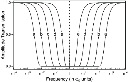
Figure 1: Amplitude transmission $\left|H(z,\omega\right|$ of the medium as a function of the frequency modulus $\lvert\omega\rvert$ (logarithmic scale). Parameters (in $\omega_{0}$ units) : $\omega_{p}=1.11$ , $\gamma=0.0707$ and $\xi=8.31\times 10^{5}$ for the curve (a) corresponding to the Brillouin choice ($z=10^{-2}\mathrm{m}$ ). The curves (b), (c),(d) and (e) are obtained for propagation distances (and thus $\xi$ ) respectively 10, 100, 1 000 and 10 000 times smaller.

Figure 1 shows the profiles of the amplitude transmission $\left|H(z,\omega)\right|)=\exp\left[-\alpha\left(\omega\right)z\right]$ as a function of the reduced frequency $\omega/\omega_{0}$ in the Brillouin conditions (curve a) and for propagation distances 10, 100, 1 000 and 10 000 times shorter (curves b to e).

The medium being opaque for $\omega_{-}<\omega<\omega_{+}$, the transfer function may be written as

$$H(z,\omega)=H_{S}(z,\omega)+H_{B}(z,\omega),$$ (7)

with $H_{S}(z,\omega)\approx 0$ for $\omega<\omega_{+}$ and $H_{B}(z,\omega)\approx 0$ for $\omega>\omega_{-}$. $H_{S}$ and $H_{B}$ are respectively associated with the Sommerfeld and the Brillouin precursor. For $\omega=0$, $H_{S}(z,0)\approx 0$ and $H_{B}(z,0)\approx H(z,0)=1$. As long as $\omega_{c}$ lies in the opacity region, this implies that the Sommerfeld precursor will have a zero area while the area of the Brillouin precursor will be equal to that of the incident field.

The formation of the optical precursors is generally governed by combined effects of attenuation (considered above) and dispersion. The dispersion effects can be soundly characterized by the group delay $\tau_{g}(z,\omega)=-d\Phi/d\omega=z/v_{g}(\omega)-z/c$, where $\Phi(z,\omega)$ is the argument of $H(z,\omega)$ and $v_{g}(\omega)$ the group velocity re2 . We remark that the regions of anomalous dispersion ($dn/d\omega<0$) or of superluminal group velocity ($\tau_{g}<0$ ) has a width smaller than $\omega_{0}$ and are entirely comprised inside the opacity region. The corresponding frequencies will thus not directly contribute to the formation of precursors. For the high and low frequencies respectively associated with the Sommerfeld and Brillouin precursors, we get the asymptotic forms $\tau_{g}\approx\xi/\omega^{2}$ re2 and $\tau_{g}\approx t_{B}+\omega^{2}/(\eta b^{3})$ where

$$t_{B}=\frac{\left[n(0)-1\right]z}{c}=\frac{2\xi}{\omega_{p}^{2}}\left[\left(1+\frac{\omega_{p}^{2}}{\omega_{0}^{2}}\right)^{1/2}-1\right]$$ (8)

$$b=\omega_{0}\left(3\frac{\xi}{\omega_{0}}\right)^{-1/3}\left(1+\frac{\omega_{p}^{2}}{\omega_{0}^{2}}\right)^{1/6}$$ (9)

$$\frac{1}{\eta}=1-\frac{4\gamma^{2}}{\omega_{0}^{2}}\left(1+\frac{3\omega_{p}^{2}}{4\omega_{0}^{2}}\right)/\left(1+\frac{\omega_{p}^{2}}{\omega_{0}^{2}}\right).$$ (10)

$t_{B}=\tau_{g}(z,0)-\tau_{g}(z,\infty)$ is obviously indicative of the time delay of the Brillouin precursor (low frequency) with respect to the Sommerfeld precursor (high frequency). The two precursors will be fully separated when $t_{B}$ is much larger than the damping time $1/\gamma$. Since $\gamma t_{B}=O\left(\gamma\xi/\omega_{0}^{2}\right)$, this condition is automatically fulfilled when the condition of broad opacity-region $\left[\gamma\xi/(10\omega_{0}^{2})\gg 1\right]$ holds. Another important point is that $\tau_{g}$ is minimum (stationary) for $\omega\rightarrow\infty$ and $\omega\rightarrow 0$. As pointed out by Brillouin bri32 , this ensures that the precursors will not be washed out by the group velocity dispersion.

III SOMMERFELD PRECURSOR

III.1 Transfer function $H_{S}(z,\omega)$ and impulse response

In the limit considered here $\omega^{2}\geq\omega_{+}^{2}\gg\omega_{0}^{2}$ and $H_{S}(z,\omega)$ takes the following asymptotic form, accounting for both dispersion (main contribution) and attenuation.

$$H_{S}(z,\omega)\approx\exp\left[-\frac{\xi}{i\omega+2\gamma}\right].$$ (11)

The corresponding impulse response $h_{S}(z,t)$ is easily determined by using standard results of Laplace transforms ab72 . We get

$$h_{S}(z,t)=\delta(t)-\sqrt{\frac{\xi}{t}}\mathrm{J}_{1}\left(2\sqrt{\xi t}\right)\mathrm{e}^{-2\gamma t}\mathrm{u}_{H}(t),$$ (12)

where $\mathrm{J}_{n}(s)$ and $\mathrm{u}_{H}(t)$ respectively designate the first kind Bessel-function of index $n$ and the Heaviside unit-step function. Except for their very first oscillation, the Bessel functions $\mathrm{J}_{n}(s)$ are perfectly approximated by their asymptotic form

$$\mathrm{J}_{n}(s)\approx\sqrt{\frac{2}{\pi s}}\cos\left(s-n\frac{\pi}{2}-\frac{\pi}{4}\right),$$ (13)

and the impulse response $h_{S}(z,t)$ can be characterized by an instantaneous frequency $\omega\approx d\left(2\sqrt{\xi t}\right)/dt=\sqrt{\xi/t}$. The range of validity of Eq.(12) may be estimated by determining the change $\delta H_{S}(z,\omega)$ of $H_{S}(z,\omega)$ due to the first term neglected in the asymptotic expansion of $\ln\left[H_{S}\left(z,\omega\right)\right]$ used to obtain Eq.(11). We find $\delta H_{S}(z,\omega)/H_{S}(z,\omega)=O\left(\xi\omega_{0}^{2}/\omega^{3}\right)$, negligible when $\omega^{3}\gg\xi\omega_{0}^{2}$, i.e. when $\xi^{1/2}\gg\omega_{0}^{2}t^{3/2}$. In fact, Eq.(12) fits very well the exact impulse response as soon as $\xi^{1/2}$ exceeds $\omega_{0}^{2}t^{3/2}$ by a factor $\sqrt{10}$ (half an order of magnitude). This is achieved as long as $t\leq t_{S}$, with

$$\omega_{0}t_{S}=\sqrt[3]{\frac{\xi}{10\omega_{0}}}.$$ (14)

In a strict asymptotic limit ($z\rightarrow\infty$), $t_{S}\rightarrow\infty$ and $\exp\left(-2\gamma t_{S}\right)\rightarrow 0$. As expected, the entirety of the impulse response is then reproduced by Eq.(12).

III.2 Precursor originated by a causal incident field

The Sommerfeld precursor $e_{S}(z,t)$ is obtained by convoluting $h_{S}(z,t)$ with the incident field $e(0,t)=u(t)\cos\left(\omega_{c}t-\varphi\right)$ introduced in the general analysis [Eq.(1)]. We are mainly interested here in the physical case where the incident field is causal [$e(0,t)=0$ for $t<0$], $u(t)$ being either a unit step $\mathrm{u}_{H}(t)$ or a function monotonously rising from $0$ to $1$ with a rate $r\lesssim\omega_{c}$ for $t>0$ (step or step-like modulation). The convolution product of Eq.(5) takes the form:

$$e_{S}(z,t)=\intop_{-\infty}^{t}h_{S}(z,\theta)e(0,t-\theta)d\theta,$$ (15)

that can be transformed by repeated integrations per parts to yield

$$e_{S}(z,t)=\sum_{n=0}^{\infty}d_{n}h_{S}^{\left(n+1\right)}(z,t).$$ (16)

Here $d_{n}$ is the discontinuity of the $\mathrm{n}^{\mathrm{th}}$ derivative of $e(0,t)$ at the initial time re3 and $f^{\left(n\right)}(t)$ is a short-hand notation for $\int_{-\infty}^{t}\int_{-\infty}^{t_{1}}\cdots\int_{-\infty}^{t_{n-1}}f(t_{n})dt_{n}\cdots dt_{2}dt_{1}$. In a frequency description, the previous result can be retrieved by expanding the Fourier transform $E(0,\omega)$ of $e(0,t)$ in powers of $1/i\omega$ and exploiting the equivalence between multiplication by $1/i\omega$ in the frequency domain and integration in the time domain pap87 . Writing the impulse response under the form $h_{S}(z,t)=k_{S}(z,t)\exp(-2\gamma t)$, we easily show by means of standard Laplace procedures ab72 that $k_{S}^{\left(n+1\right)}(z,t)=(t/\xi)^{n/2}\mathrm{J}_{n}(2\sqrt{\xi t})\mathrm{u}_{H}(t)$. Insofar as $k_{S}(z,t)$ is very rapidly varying compared to $\exp(-2\gamma t)$, $h_{S}^{\left(n+1\right)}(z,t)\approx k_{S}^{\left(n+1\right)}(z,t)\exp(-2\gamma t)$ and we finally get

$$e_{S}(z,t)\approx\sum_{n=0}^{\infty}d_{n}\left(\frac{t}{\xi}\right)^{n/2}\mathrm{J}_{n}(2\sqrt{\xi t})\exp\left(-2\gamma t\right)\mathrm{u}_{H}(t).$$ (17)

The $\mathrm{n^{th}}$ term of the series has a maximal amplitude $a_{0}=\left|d_{0}\right|$ at $t=t_{0}=0$ for $n=0$ and

$$a_{n}=\frac{1}{\sqrt{\pi}}\left|d_{n}\right|\left(\frac{2n-1}{8\mathrm{e}}\right)^{\left(2n-1\right)/4}\left(\frac{\gamma}{\xi}\right)^{1/4}\left(\gamma\xi\right)^{-n/2},$$ (18)

at $t\approx t_{n}=\left(2n-1\right)/8\gamma$ for $n>0$. Since $\xi\propto z$, Eq.(18) shows that, for large propagation distance, $a_{n}$ rapidly decreases with $n$, so that a good approximation of the exact result is obtained by keeping only the first term $n=p$ of the series for which $d_{p}\neq 0$. In the frequency description, this amounts to restrict the asymptotic expansion of $E(0,\omega)$ to its first non vanishing term ja75 . We then get

$$e_{S}(z,t)\approx d_{p}\left(\frac{t}{\xi}\right)^{p/2}\mathrm{J}_{p}(2\sqrt{\xi t})\exp\left(-2\gamma t\right)\mathrm{u}_{H}(t).$$ (19)

Denoting $q$ is the next integer following $p$ for which $d_{q}\neq 0$, Eq.(19) is exact when $\varepsilon=a_{q}/a_{p}\approx 0$, and $\exp\left(-2\gamma t_{S}\right)\approx 0$. These conditions are met in the strict asymptotic limit and closely approached for the propagation distance considered by Brillouin. At distances that may be 1 000 times smaller (simple asymptotic limit); we shall see that Eq.(19) enables us to correctly reproduce the essential features of the precursor originated by representative incident fields.

III.3 Precursor originated by a discontinuous incident field

We consider first the instructive case where $e(0,t)=u_{H}(t)\cos\left(\omega_{c}t\right)$ for which $p=0$ with $d_{0}=1$ re3 and $q=2$ with $d_{2}=-\omega_{c}^{2}$. Eq.(19) then reads as

$$e_{S}(z,t)\approx\mathrm{J_{0}}(2\sqrt{\xi t})\exp\left(-2\gamma t\right)\mathrm{u}_{H}(t),$$ (20)

with $\varepsilon\approx 0.13\omega_{c}^{2}\gamma^{-3/4}\xi^{-5/4}$ [see Eq. 18]. The precursor does not depend on $\omega_{c}$ and the initial discontinuity of the incident field is integrally transmitted, in agreement with the general analysis. For $\omega_{c}<\omega_{+}=\sqrt{\gamma\xi/10}$ (opacity condition), $\varepsilon$ is always smaller than $0.013\left(\gamma/\xi\right)^{1/4}$, that is about $2.2\times 10^{-4}$ in the Brillouin conditions and $1.2\times 10^{-3}$ for a propagation distance 1 000 times smaller (simple asymptotic limit). In the first case, $\omega_{0}t_{S}=44$ and $\exp\left(-2\gamma t_{S}\right)\approx 2\times 10^{-3}$. As previously indicated, we are then close to the strict asymptotic limit and the precursor is perfectly reproduced by its asymptotic form at any time where it has a significant amplitude.

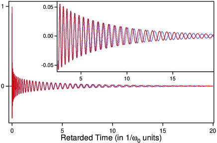
Figure 2: Sommerfeld precursor originated by the incident field $\cos(\omega_{c}t)\mathrm{u}_{H}(t)$. The solid (dashed) line is the exact numerical solution (the approximate analytic solution). Parameters (in $\omega_{0}$ units) : $\omega_{c}=1$, $\omega_{p}=1.11$, $\gamma=0.0707$ and $\xi=831$. Inset : enlargement of the tail of the precursor.

This remark also holds for the cases considered in the following subsections. In the simple asymptotic limit $\omega_{0}t_{S}=4.4$ and, as expected, Eq.(20) perfectly fits the exact solution for $\omega_{0}t\leq 4.4$. For larger times, the fit remains very good except for a slight drift of the instantaneous frequency of the oscillations whose envelope is very well reproduced at any time (Fig.2).

III.4 Precursor originated by the canonical incident field of Sommerfeld and Brillouin

Following Sommerfeld and Brillouin, most authors have considered an incident field of the canonical form $e(0,t)=u_{H}(t)\sin\left(\omega_{c}t\right)$ for which $p=1$ with $d_{1}=\omega_{c}$ and $q=3$ with $d_{3}=-\omega_{c}^{3}$. We then get

$$e_{S}(z,t)\approx\omega_{c}\sqrt{\frac{t}{\xi}}\mathrm{J_{1}}(2\sqrt{\xi t})\exp\left(-2\gamma t\right)\mathrm{u}_{H}(t),$$ (21)

with $\varepsilon\approx 0.34\left(\omega_{c}^{2}/\gamma\xi\right)$. The result given Eq.(21) differs from that originally obtained by Sommerfeld som14 by the presence of the damping term $\exp\left(-2\gamma t\right)$ . Though the formation of the Sommerfeld precursor is mainly governed by the medium dispersion, the presence of this term (associated with the absorption) is obviously necessary to avoid that $e_{S}(z,t)$ diverges with time. The precursor attains its maximum at $t\approx t_{1}=1/\left(8\gamma\right)$ ($\omega_{0}t_{1}=1.77$ ) and its amplitude $a_{S}=a_{1}\approx 0.26\>\omega_{c}\gamma^{-1/4}\xi^{-3/4}$ is proportional to $\omega_{c}$. For $\omega_{c}=\omega_{0}$, $a_{S}\approx 1.8\times 10^{-5}$ with $\varepsilon\approx 5.8\times 10^{-6}$ in the Brillouin conditions whereas $a_{S}\approx 3.25\times 10^{-3}$ with $\varepsilon\approx 5.8\times 10^{-3}$ in the simple asymptotic limit. In the latter case, Fig.3 shows that Eq.(21) actually fits very well the exact result for $t\leq t_{S}$, again with a slight drift of the instantaneous frequency of the oscillations for $t>t_{S}$. In order to check the proportionality of the precursor to $\omega_{c}$, we have compared the exact forms of $\left(\omega_{0}/\omega_{c}\right)\>e_{S}(z,t)$ obtained when $\omega_{c}$ lies at the boundaries $\omega_{-}$ or $\omega_{+}$ of the opacity region to that obtained when $\omega_{c}=\omega_{0}$. As expected we have found that the three results are nearly undistinguishable, except for an amplitude $1.3\%$ larger for $\omega_{c}=\omega_{+}$ (below the corresponding value of $\epsilon$, namely $\varepsilon=0.034$). For this value of $\omega_{c}$, the amplitude of the precursor is $a_{S}\approx 0.082\left(\gamma/\xi\right)^{1/4}$, that is $1.40\times 10^{-3}$ in the Brillouin conditions and $7.9\times 10^{-3}$ in the simple asymptotic limit.

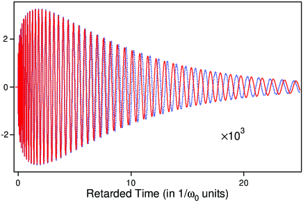
Figure 3: Sommerfeld precursor originated by the canonical incident field $\sin(\omega_{c}t)\mathrm{u}_{H}(t)$. The solid (dashed) line is the exact numerical solution (the approximate analytic solution). Parameters as in Fig.2.

III.5 Rise-time effects

A gradual turning on of the incident field is expected to reduce the amplitude of the Sommerfeld precursor. To study this so-called rise-time effect, Ciarkowski cia02 ; cia11 has considered the incident field $e(0,t)=\tanh\left(rt\right)\sin\left(\omega_{c}t\right)\mathrm{u}_{H}(t)$ whose envelope has a $10-90\%$ rise time $T_{r}\approx 1.37/r$. In this case $p=2$ with $d_{2}=2r\omega_{c}$, $q=4$ with $d_{4}=-4\omega_{c}r\left(2r^{2}+\omega_{c}^{2}\right)$ and the asymptotic form of the precursor reads as

$$e_{S}(z,t)\approx 2\omega_{c}r\left(\frac{t}{\xi}\right)\mathrm{J}_{2}(2\sqrt{\xi t})\exp\left(-2\gamma t\right)\mathrm{u}_{H}(t),$$ (22)

with $\varepsilon\approx 1.21\left(2r^{2}+\omega_{c}^{2}\right)/\gamma\xi$. The precursor attains its maximum at $t\approx t_{2}=3/(8\gamma)$ ($\omega_{0}t_{2}\approx 5.3$) with an amplitude $a_{S}=a_{2}\approx 0.26\>r\omega_{c}\gamma^{-3/4}\xi^{-5/4}$. Compared to the precursor obtained with the canonical incident field [Eq.(21)], the maximum is shifted to larger time ($t_{2}=3t_{1}$) and its amplitude is reduced by a factor $\rho\approx\sqrt{\gamma\xi}$/r. Fig.4, obtained in the simple asymptotic limit, shows that Eq.(22) fits quite satisfactorily the exact precursor though its maximum now lies at a time slightly larger than $t_{S}$. To check that the precursor is mainly determined by the lowest order initial discontinuity of the incident field regardless of its subsequent evolution, we have compared the precursor obtained when the envelope $\tanh\left(rt\right)u_{H}(t)$ is replaced by $\left(1-\mathrm{e}^{-rt}\right)u_{H}(t)$, having the same initial discontinuity. Though $q=3$ (instead of $4$) and $T_{r}\approx 2.20/r$ (instead of $1.37/r$), we have found that the precursor is actually very close to the previous one.

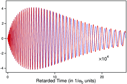
Figure 4: Sommerfeld precursor originated by the incident field $e(0,t)=\tanh(rt)\>\sin(\omega_{c}t)\>u_{H}(t)$. The solid (dashed) line is the exact numerical solution (the approximate analytic solution) obtained for $r=\omega_{0}$. Other parameters as in Fig.2.

Other things being equal, the reduction of the amplitude of the precursor is more and more important when the incident field is applied more and more smoothly, that is when the order $p$ of its initial discontinuity increases. It is easily deduced from Eq.(18) that for $p\geq 2$, $\rho=O\left[\left(\sqrt{\gamma\xi}/r\right)^{p-1}\right]\propto\left(T_{r}\sqrt{z}\right)^{p-1}$. At the light of this result, dramatic rise time effects are expected when the incident field is ideally smooth, i.e. analytic with continuous derivatives in every point. Such fields have been considered ou09 ; bm11 ; ou95 though they are not causal and, strictly speaking, not physically realizable (in the sense of the linear systems theory). We have made numerical simulations for $e(0,t)=\sin\left(\omega_{c}t\right)\left[1+\mathrm{erf}\left(rt\right)\right]/2$ where $\mathrm{erf}(s)$ designates the error function. For $z$ and $r=\omega_{0}$ as in Fig.4, we get $\rho\approx 1.4\times 10^{3}$ instead of $\rho\approx 7.7$ for $e(0,t)=\tanh(rt)\>\sin(\omega_{c}t)\>u_{H}(t)$.

IV BRILLOUIN PRECURSOR IN THE STRICT ASYMPTOTIC LIMIT

IV.1 Transfer function $H_{B}(z,\omega)$ and impulse response

In the limit considered now $\omega^{2}\leq\omega_{-}^{2}\ll\omega_{0}^{2}$ and $H_{B}(z,\omega)$ is conveniently developed under the form

$$H_{B}(z,\omega)=\exp\left(\sum_{n=1}^{\infty}\frac{\left(-i\omega\right)^{n}}{n!}k_{n}(z)\right).$$ (23)

Here $k_{n}(z)$ are the so-called cumulants, generally introduced in probability theory ab72 , but also quite useful to study deterministic signals bu04 ; bm06 . The cumulants $k_{1}(z)$, $k_{2}(z)$ and $k_{3}(z)$ have remarkable properties. $k_{1}(z)$ and $k_{2}^{1/2}(z)$ respectively are the center-of-mass and the root-mean-square duration of the impulse response $h_{B}(z,t)$, inverse Fourier transform of $H_{B}(z,\omega)$, whereas $\kappa(z)=k_{3}(z)/k_{2}^{3/2}(z)$ is its normalized asymmetry or skewness ab72 . From Eqs.(3,4), we easily get $k_{1}=t_{B}$ (as expected), $k_{2}=4\gamma/(3b^{3})$ , $k_{3}=-2/(\eta b^{3})$ and $\kappa=-(1/4\eta)\left(3b/\gamma\right)^{3/2}$, where $t_{B}$, $b$ and $\eta$ are defined by Eqs.(8-10). When $z\rightarrow\infty$ (strict asymptotic limit), $\kappa\propto b^{3/2}\propto z^{-1/2}\rightarrow 0$ and the expansion of Eq.(23) may be limited to the term $n=2$. Taking a new origin of time at $t=t_{B}$, the transfer function then reads as

$$H_{B}(z,\omega)\approx\exp\left(-\frac{\omega^{2}}{4\beta^{2}}\right),$$ (24)

where $\beta=\sqrt{3b^{3}/8\gamma}\propto 1/\sqrt{z}$ is very small compared to $\omega_{0}$. This Gaussian form is that of the normal distribution derived by means of the central limit theorem in probability theory. This theorem can also be used to obtain an approximate evaluation of the convolution of $n$ deterministic functions pap87 . It can be applied to our case by splitting the medium into $n$ cascaded sections, $h_{B}(z,t)$ being the convolution of the impulses responses of each section. By calculating the inverse Fourier transform of $H_{B}(z,\omega)$, we get

$$h_{B}(z,t)=\frac{\beta}{\sqrt{\pi}}\exp\left(-\beta^{2}t^{\prime 2}\right),$$ (25)

where $t^{\prime}=t-t_{B}$. The impulse response has a duration (amplitude) proportional (inversely proportional) to $\sqrt{z}$, with an area constantly equal to $1$ (in agreement with the general analysis). We remark that the approximation leading to Eq.(24) and Eq.(25), valid in the strict asymptotic limit, amounts to neglect the effects of the group delay dispersion, the formation of the Brillouin precursor being then governed by the frequency dependence of the medium attenuation (dominant-attenuation limit).

The Gaussian forms of Eq.(24) and Eq.(25) are not specific to the Lorentz medium but have some generality kla05 . They hold for the Debye medium sto01 , for some random media ga10 and, more generally, whenever the transfer function of the medium can be expanded in cumulants and the propagation distance is such that $\left|\kappa\right|\ll 1$. Stoudt et al. sto01 showed in particular that the results of their experiments on water (Debye medium) at decimetric wavelengths can be numerically reproduced by neglecting the group delay dispersion, as it has been made to obtain Eq.(24). See also ou05 ; pi09 ; da10 ; ca11 . Using a purely temporal approach, Karlsson and Ritke ka98 early remarked that the impulse response of the Debye medium is very close to a normalized Gaussian. This property is obviously a consequence of the previous analysis. The complex refractive index now reads as $\widetilde{n}(\omega)=\left[1+\left(n_{0}^{2}-1\right)/\left(1+i\omega\tau\right)\right]^{1/2}$ where $n_{0}$ is the refractive index for $\omega\rightarrow 0$ and $\tau$ is the relaxation time for the orientation of the polar molecules pi09 . Including $\widetilde{n}(\omega)$ in Eq.(3) and following the procedure used for the Lorentz medium, we easily get $\beta=\left[2\left(n_{0}^{2}-1\right)\tau z/cn_{0}\right]^{-1/2}$ and, taking into account that $n_{0}^{2}\gg 1$, $\kappa\approx 2.25\sqrt{c\tau/n_{0}z}$. Note that $\beta$ and $\kappa$ depends on $z$ as $1/\sqrt{z}$ (as in the Lorentz medium). The normalized Gaussian of Eq.(25) will thus also be obtained for sufficient propagation distances. Using the parameters of water pi09 , namely $n_{0}=\sqrt{79}$ and $\tau=8.5\times 10^{-12}\mathrm{s}$, we find that the skewness of $5.2\%$, obtained in a Lorentz medium for a propagation distance larger by more of four orders of magnitude than the optical wavelengths considered, is now attained for a propagation distance $z\approx 0.55\>\mathrm{m}$ comparable to the wavelengths involved in the experiments reported in sto01 . Despite strongly different scales, Brillouin precursors in the Lorentz medium in the strict asymptotic limit and in the Debye medium pertain to the same physics, namely that of the dominant-attenuation limit, and will be described by the same laws. On the other hand, the Debye medium is fully opaque at high frequency and Sommerfeld precursors cannot be generated in this medium.

IV.2 Precursor generated by an incident field of non-zero area

The Brillouin precursor generated by an arbitrary incident field $e(0,t)$ is obtained by convoluting the latter with $h_{B}(z,t)$ or by multiplying its Fourier transform $E(0,\omega)$ by $H_{B}(z,\omega)$ and determining the inverse Fourier transform of the product. We consider first the case where $e(0,t)$ is rapidly varying compared to $h_{B}(z,t)$. This requires in particular that $\omega_{c}\gg\beta$. Compared to $E(0,\omega)$, $H_{B}(z,\omega)$ then appears as a narrow peak centered on $\omega=0$ and, provided that $E(0,0)\neq 0$, $E_{B}(z,\omega)\approx E(0,0)\>H_{B}(z,\omega)$. Remembering that $E(0,0)$ is the algebraic area $\mathcal{A}$ of the incident field (see Sec. II), we finally get:

$$e_{B}(z,t)\approx\mathcal{A}h_{B}(z,t)=\frac{\mathcal{A\beta}}{\sqrt{\pi}}\exp\left(-\beta^{2}t^{\prime 2}\right).$$ (26)

For the canonical incident field $\sin\left(\omega_{c}t\right)\mathrm{u}_{H}(t)$, $E(0,0)=1/\omega_{c}$ and the precursor has an amplitude $a_{B}=\beta/\left(\omega_{c}\sqrt{\pi}\right)$ inversely proportional to $\omega_{c}$ (no matter its value provided that $\omega_{c}\gg\beta$) and to $\sqrt{z}$. Note that the law $a_{B}\propto 1/\sqrt{z}$, sometimes considered as general, is only valid in the strict asymptotic limit considered here (for which $\left|\kappa\right|\ll 1$).

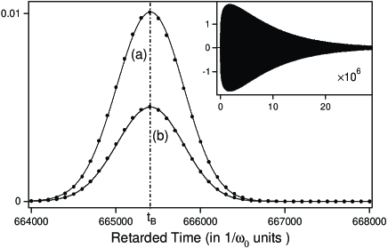
Figure 5: Brillouin precursor obtained in the Brillouin conditions, namely for $\omega_{c}=0.1$, $\omega_{p}=1.11$, $\gamma=0.0707$ and $\xi=8.31\times 10^{5}$ (in $\omega_{0}$ units). For these parameters, $\omega_{0}t_{B}\approx 6.654\times 10^{5}$ and $\beta\approx 1.78\times 10^{-3}\omega_{0}=1.78\times 10^{-2}\omega_{c}$. Solid lines (bullets $\bullet$) are the exact numerical solutions (the analytic solutions). Curve (a) is the precursor obtained with the canonical incident field $\sin(\omega_{c}t)u_{H}(t)$. The precursor of curve (b) is originated by the incident field $e(0,t)=\sin(\omega_{c}t)\left[1+\textrm{erf}(rt)\right]/2$ for $r=\omega_{c}/2\sqrt{2}$ . Inset: Sommerfeld precursor obtained in the conditions of curve (a). It fully vanishes in the conditions of curve (b).

Fig.5 shows that the precursor obtained in all the Brillouin conditions [curve (a)] is perfectly fitted by the Gaussian form of Eq.(26). We incidentally note that, for the carrier frequency retained by Brillouin ($\omega_{c}=\omega_{0}/10$), the medium is fully opaque at this frequency [$\alpha\left(\omega_{c}\right)z\approx 800$], in contradiction with his artist’s view showing a “main field” (at $\omega_{c}$) larger than the precursors. On the other hand, the condition $\omega_{c}\gg\beta$ is well satisfied. The inset in Fig.5 shows the Sommerfeld precursor obtained in the same conditions. As already mentioned, it is perfectly fitted by the analytical expression of Eq.(21). Note however that its amplitude is about four orders of magnitude smaller than that of the Brillouin precursor. Eq.(26) also holds when the envelope of the incident field rises in a finite time provided that the rate $r$ , as $\omega_{c}$, is large compared to $\beta$. Curve (b) of Fig.5 shows the Brillouin precursor generated by the incident field $e(0,t)=\sin\left(\omega_{c}t\right)\left[1+\mathrm{erf}\left(rt\right)\right]/2$. We have then $E(0,0)=(1/\omega_{c})\exp\left(-\omega_{c}^{2}/4r^{2}\right)$ and the area of the incident pulse, equal to $1/\omega_{c}$ for $r\rightarrow\infty$, falls to $1/2\omega_{c}$ for $r=\omega_{c}/2\sqrt{\ln\left(2\right)}$ ($r\approx 0.60\omega_{c}$). As expected, the Brillouin precursor is identical to the previous one with amplitude reduced by half and the corresponding Sommerfeld precursor completely vanishes.

IV.3 Precursor originated by an incident field of zero area

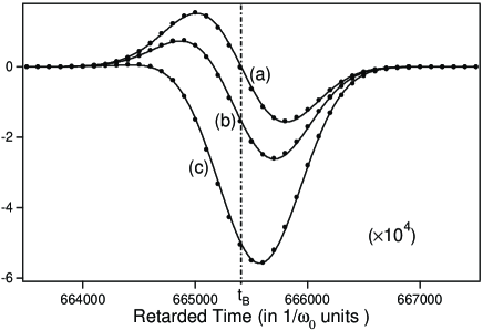
Figure 6: Brillouin precursor obtained with the incident fields $(1-\mathrm{e}^{-rt})\cos(\omega_{c}t)\mathrm{u}_{H}(t)$ for (a) $r\rightarrow\infty$, (b) $r=65\omega_{c}$ and (c) $r=20\omega_{c}$ (solid lines). Other parameters as in Fig.5. The bullets $\bullet$ correspond to the analytical solutions given by Eq.(27) or by the combination of this equation with Eq.(26).

Even if $\omega_{c},r\gg\beta$, Eq.(26) obviously fails when $\mathcal{A}=E(0,0)=0$. This occurs in particular in the extreme case where the incident field is instantaneous turned on, with $e(0,t)=\cos\left(\omega_{c}t\right)\mathrm{u}_{H}(t)$. It is then necessary to consider the next term in the expansion of $E(0,\omega)$ in powers of $i\omega$. We get in this case $E(0,\omega)\approx i\omega/\omega_{c}^{2}$ and $E_{B}(z,\omega)\approx i\omega H_{B}(z,\omega)/\omega_{c}^{2}$. Using the correspondence $i\omega\leftrightarrow d/dt$ between frequency and time descriptions pap87 and denoting by a dot the time derivative, we finally get:

$$e_{B}(z,t)\approx\frac{1}{\omega_{c}^{2}}\overset{.}{h_{B}}(z,\omega t)=-\frac{2\beta^{2}}{\omega_{c}^{2}\sqrt{\pi}}\>\beta t^{\prime}\exp\left(-\beta^{2}t^{\prime 2}\right).$$ (27)

As shown Fig.6 [curve (a)], the analytical expression of Eq.(27) perfectly fits the exact numerical results obtained by FFT. The precursor is a Gaussian derivative with a peak amplitude $a_{B}=\left[2/(\pi\mathrm{e})\right]^{1/2}\left(\beta/\omega_{c}\right)^{2}$, smaller than that attained with the canonical incident field by a factor $\omega_{c}\sqrt{\mathrm{e}}/(\beta\sqrt{2})$ ($\approx 65$ in all the Brillouin conditions) and decreasing much more rapidly with the propagation distance (as $1/z$ instead of as $1/\sqrt{z}$). We however remark that the precursor so obtained is not robust. Indeed it suffices that the incident field suffers a short rise time to retrieve a precursor mainly governed by the area law of Eq.(26). To illustrate this point, we have again considered an incident field of the form $\left(1-\mathrm{e}^{-rt}\right)\cos\left(\omega_{c}t\right)\mathrm{u}_{H}(t)$ that tends to $\cos\left(\omega_{c}t\right)\mathrm{u}_{H}(t)$ for $r\rightarrow\infty$. For $r\gg\omega_{c}$ (very short rise time), $E(0,\omega)\approx-1/r+i\omega/\omega_{c}^{2}$. The incident field has gained a (negative) area $\mathcal{A}=-1/r$. The precursor is then the sum of two contributions, respectively given by Eq.(26) with $\mathcal{A}=-1/r$ and by Eq.(27). Curve (b) of Fig.6 shows the result obtained when the two contributions have the same amplitude, that is when $r/\omega_{c}=\omega_{c}\sqrt{\mathrm{e}}/(\beta\sqrt{2})\approx 65$ . When $r$ decreases by remaining large compared to $\omega_{c}$, the Gaussian part of the precursor rapidly prevails on the Gaussian-derivative part and, as shows [curve (c)], the precursor becomes nearly Gaussian (downwards) for $r$ as large as $20\omega_{c}$.

IV.4 Case where the carrier frequency lies below the opacity region

The previous results are valid for the Lorentz medium in the strict asymptotic limit (also as in the Debye medium) when $\omega_{c}\gg\beta$, that is when $\omega_{c}$ lies in the opacity region. Fortunately enough, the simplicity of the Gaussian impulse response enables us to obtain exact expressions of the transmitted field for arbitrary values of the ratio $\omega_{c}/\beta$. This occurs in the Lorentz medium when $\omega_{c}$ resides below the opacity region and direct observations of the field transmitted in such conditions have been performed by Stoudt et al. in a Debye medium sto01 . The transmitted field $e(z,t)$ is calculated directly in the time domain by convoluting $h_{B}(z,t)$ given Eq.(25) with the incident field. For the canonical incident field, the convolution product can be written as:

$$e(z,t)=\frac{\beta}{\sqrt{\pi}}\intop_{-\infty}^{t^{\prime}}\mathrm{e}^{-\beta^{2}\theta^{2}}\sin\left[\omega_{c}\left(t^{\prime}-\theta\right)\right]d\theta.$$ (28)

After some simple transformations, we finally get

$$e(z,t)=\frac{1}{2}\>\mathrm{e}^{-\omega_{c}^{2}/4\beta^{2}}\Im\left\{\left[1+\mathrm{erf}\left(\beta t^{\prime}+\frac{i\omega}{2\beta}\right)\right]\>\mathrm{e}^{i\omega_{c}t^{\prime}}\right\}$$ (29)

where $\mathrm{e}^{-\omega_{c}^{2}/4\beta^{2}}\approx\mathrm{e}^{-\alpha\left(\omega_{c}\right)z}$ and, as previously, $t^{\prime}=t-t_{B}$. For $t^{\prime}\rightarrow\infty$, $e(z,t)$ tends to $\mathrm{e}^{-\omega_{c}^{2}/4\beta^{2}}\sin\left(\omega_{c}t^{\prime}\right)$ which is nothing but that the steady state or main field, not negligible when $\omega_{c}$ and $\beta$ are comparable. If we take $t_{B}$ ($1/\beta$) as time origin (time unit), the transmitted field only depends on the ratio $\omega_{c}/\beta$, regardless of the particular system considered. When $\omega_{c}\gg\beta$, it tends to $\beta/\left(\omega_{c}\sqrt{\pi}\right)\exp\left(-\beta^{2}t^{\prime 2}\right)$ in agreement with Eq.(26), the main field being then negligible. When $\omega_{c}\geq 4\beta$, Eq.(29) is well approximated by the expression:

$$e(z,t)\approx\frac{1+\mathrm{erf}\left(\beta t^{\prime}\right)}{2}\>\sin\left(\omega_{c}t^{\prime}\right)\>\mathrm{e}^{-\alpha\left(\omega_{c}\right)z}+\\ \frac{\beta^{\prime}}{\omega_{c}\sqrt{\pi}}\>\mathrm{e}^{-\beta^{\prime 2}t^{\prime 2}},$$ (30)

where $\beta^{\prime}=\beta\left(1+2\beta^{2}/\omega_{c}^{2}\right)\rightarrow\beta$ for $\omega_{c}\gg\beta$. The first (second) term of Eq.(30) obviously corresponds to the main field (the Brillouin precursor). Figure 7 shows the transmitted field as a function of $\beta t^{\prime}=\beta\left(t-t_{B}\right)$ for $\omega_{c}\approx 3.84\beta$ and $\omega_{c}\approx 7.67\beta$ (inset). In the study on water (Debye medium) at decimetric wavelengths sto01 , these values are obtained with $\omega_{c}=2\pi\times 10^{9}\>\mathrm{s}^{-1}$, for $z=0.75\>\mathrm{m}$ and $z=3\>\mathrm{m}$ respectively. As expected Eq.(29) perfectly fits the exact numerical result in both cases. Eq.(30) provides a good approximation for $\omega_{c}\approx 3.84\beta$, excellent for $\omega_{c}\approx 7.67\beta$. In the latter case, the Brillouin precursor prevails over the main field whose relative amplitude is negligible. The signals shown Fig.7 are in good agreement with those directly observed in the experiments reported in sto01 .

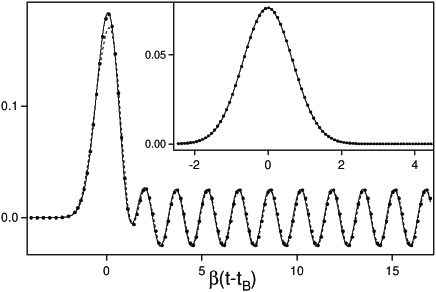
Figure 7: Brillouin precursor and main field obtained for $\omega_{c}\approx 3.84\beta$ as a function of $\beta(t-t_{B})$. The solid line, the bullets $\bullet$ and the dashed line are respectively the exact numerical solution, the analytical solution given Eq.(29) and its approximate form given Eq.(30). Inset: Brillouin precursor obtained for $\omega_{c}\approx 7.67\beta$. The two analytical solutions are undistinguishable in this case and the amplitude of the main field is negligible.

V EXTENDED EXPRESSION OF THE BRILLOUIN PRECURSOR

We come back in this section to the Brillouin precursor in the Lorentz medium. Numerical simulations show that the solutions obtained in the strict asymptotic or dominant-attenuation limit continue to provide good (not too bad) approximations of the exact solutions when the propagation distance is $10$ times ($100$ times) shorter than that considered by Brillouin re1 , though the skewness $\kappa$ then rises up to $16\%$ ($52\%$). For shorter distances, it is obviously necessary to take into account the effects of the group-delay dispersion neglected in the strict asymptotic approximation.

V.1 Transfer function $H_{B}(z,\omega)$ and impulse response

Taking into account the term in $\omega^{3}$ in Eq. (23), the transfer function then reads as

$$H_{B}(z,\omega)\approx\exp\left[-i\omega t_{B}-\frac{i}{3\eta b^{3}}\left(\omega^{3}-2i\eta\gamma\omega^{2}\right)\right],$$ (31)

where $t_{B}$, $b$ and $\eta$ are defined by Eqs.(8-10), with $2\gamma/(3b^{3})=1/4\beta^{2}$. Remarking that $\left(\omega^{3}-2i\eta\gamma\omega^{2}\right)$ is the beginning of $\left(\omega-2i\eta\gamma/3\right)^{3}$ and taking a new origin of time at $t_{B}+4\eta\gamma^{2}/9b^{3}$, we get:

$$H_{B}(z,\omega)\approx\exp\left[-\frac{i}{3\eta b^{3}}\left(\omega-\frac{2}{3}i\eta\gamma\right)^{3}-\frac{\eta^{2}}{3}\left(\frac{2\gamma}{3b}\right)^{3}\right].$$ (32)

By means of an inverse Fourier transform, we finally find:

$$h_{B}(z,t)\approx B\>\mathrm{Ai}\left(-\eta^{1/3}bt"\right)\exp\left(-2\eta\gamma t"/3\right).$$ (33)

Here $B=\eta^{1/3}b\>\exp\left[-(\eta^{2}/3)\left(2\gamma/3b\right)^{3}\right]$, $t"=t-t_{B}-4\eta\gamma^{2}/9b^{3}$ and $\mathrm{Ai}(s)$ designates the Airy function. The range of validity of Eq.(33) can be roughly estimated by means of a strategy similar to that used for the Sommerfeld precursor. By taking account of the cumulants $k_{4}$ (correction of the attenuation) and $k_{5}$ (correction of the dispersion), the transfer function associated with the Brillouin precursor approximately reads as $H_{B}(z,\omega)\times\left(1-a_{4}\omega^{4}-ia_{5}\omega^{5}\right)$ where $a_{4}=-k_{4}/24>0$ and $a_{5}=k_{5}/120>0$ . $H_{B}(z,\omega)$ will be a good approximation if $a_{4}\omega^{4}$ and $a_{5}\omega^{5}$ are small compared to $1$ (say $\leq 1/\sqrt{10}$). For sake of simplicity, we take for the ratios $\omega_{p}/\omega_{0}$ and $\gamma/\omega_{0}$ the values retained by Brillouin, representative of a dense Lorentz medium with moderate damping. We get then $\eta\approx 1.018\approx 1$. Besides, in a cavalier manner, we assimilate $\omega$ to the instantaneous frequency derived from the asymptotic form $\mathrm{Ai}(-s)\approx\pi^{-1/2}s^{-1/4}\sin\left(2s^{3/2}/3+\pi/4\right)$ that provides a good approximation of $\mathrm{Ai}(-s)$ when $s>1$. We get so $\omega\approx\sqrt{b^{3}t"}$. With all these hypotheses, we finally find that the corrections due to the cumulants $k_{4}$ and $k_{5}$ will be small if $\omega_{0}t"\leq 2\left(\omega_{0}/b\right)^{3/2}$ and $\omega_{0}t"\leq\left(\omega_{0}/b\right)^{9/5}$, respectively. Despite the roughness of the procedure leading to these conditions, it will appear below that they are realistic and even too severe.

V.2 Precursor generated by the canonical incident field

When $h_{B}(z,t)$ is slowly varying compared to $e(0,t)$, the Brillouin originated by the canonical incident field $\sin\left(\omega_{c}t\right)\mathrm{u}_{H}(t)$ takes again the simple form $e_{B}(z,t)=\mathcal{A\>}h_{B}(z,t)$, that is

$$e_{B}(z,t)\approx\frac{B}{\omega_{c}}Ai\left(-\eta^{1/3}bt"\right)\exp\left(-2\eta\gamma t"/3\right).$$ (34)

It is assumed by writing Eq.(34) that the instantaneous frequency $\sqrt{b^{3}t"}$ is small compared to $\omega_{c}$ (say $\sqrt{b^{3}t"}\leq\omega_{c}/\sqrt{10}$) and that the conditions of validity of $h_{B}(z,t)$ are met. All these restrictions are summarized by the inequality

$$\omega_{0}t"\leq\min\left[2\left(\omega_{0}/b\right)^{3/2},\>\left(\omega_{0}/b\right)^{9/5},\>\omega_{0}\omega_{c}^{2}/10b^{3}\right].$$ (35)

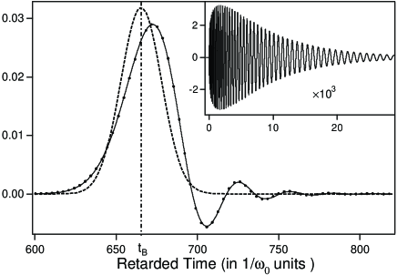
Figure 8: Brillouin precursor obtained in the simple asymptotic limit with the canonical incident field $\sin(\omega_{c}t)u_{H}(t)$. Parameters (in $\omega_{0}$ units): $\omega_{c}=1$, $\omega_{p}=1.11$, $\gamma=0.0707$ and $\xi=831$, leading to $\omega_{0}t_{B}\approx 665.4$, $b\approx 8.44\times 10^{-2}\omega_{0}$ and $\beta\approx 5.64\times 10^{-2}\omega_{0}$. The solid line, the bullets $\bullet$ and the dashed line are respectively the exact numerical solution, the analytical solution given Eq.(34) and the Gaussian that would be obtained in the dominant-attenuation approximation. The conditions are those of Fig.3. The corresponding Sommerfeld precursor is given in inset for reference.

Fig.8 shows the Brillouin precursor obtained in the simple asymptotic limit considered in the study of the Sommerfeld precursor (Fig.3). The inequality of Eq.(35) then leads to $\omega_{0}t\leq\min\left[750,\>760,\>840\right]$ . Insofar as the amplitude of the precursor is negligible for $\omega_{0}t=750$, the analytical expression of Eq.(34) perfectly fits the exact numerical result.

Surprisingly enough, Eq.(34) remains a not too bad approximation of the exact result even when the opacity region is not broad in the sense given to this expression in the present paper. Fig.9 shows the precursor obtained at a distance ten times smaller than the previous one. Though the width of the opacity region is then of the order of $\omega_{0}$ [see curve (e) of Fig.1], the entirety of the first oscillation of the Brillouin precursor is very well fitted by Eq.(34). The corresponding Sommerfeld precursor (inset) is itself well reproduced by Eq.(21) up to its maximum.

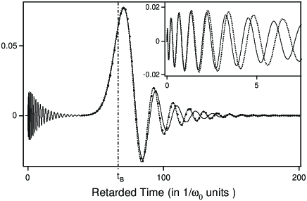
Figure 9: Comparison of the Brillouin precursor obtained outside the asymptotic limit (solid line) with the analytical forms given Eq.(34) ($\bullet$) and Eq.(36) (dashed line). Parameters (in $\omega_{0}$ units): $\omega_{c}=1$, $\omega_{p}=1.11$, $\gamma=0.0707$ and $\xi=83.1$, leading to $\omega_{0}t_{B}\approx 66.54$, $b\approx 0.182\omega_{0}$ and $\beta\approx 0.178\omega_{0}$. Inset: corresponding Sommerfeld precursor (solid line) compared to the analytic form given Eq.(21) (dashed line).

V.3 Dominant-dispersion limit

The expression of the Brillouin precursor given by Eq.(34) obviously includes as particular case the Gaussian obtained in the dominant-attenuation limit. In fact, retrieving the Gaussian precursor directly from Eq.(34) requires long and tedious calculations and this probably explains why the Gaussian solution has been generally overlooked. An other particular form of Eq.(34), also of special importance, is that obtained when the damping is very small, so that the formation of the Brillouin precursor is mainly governed by the group delay dispersion (dominant-dispersion limit). This requires in particular that $\gamma\ll b$. We then get $t"\approx t-t_{B}$, $B\approx b$ and

$$e_{B}(z,t)\approx\frac{b}{\omega_{c}}Ai\left[-b\left(t-t_{B}\right)\right]\exp\left[-\frac{2}{3}\gamma\left(t-t_{B}\right)\right].$$ (36)

Except for the exponential damping term, this result was established by Brillouin himself by means of the method of stationary phase bri32 ; re4 . When the group-delay dispersion is fully dominant (say when $\gamma/b<1/100$), the precursor has a well marked oscillatory behavior with a very weak damping and its maximum practically coincides with the first maximum of $Ai\left[-b\left(t-t_{B}\right)\right]$, attained for $t-t_{B}\approx 1,02/b$. The corresponding amplitude is $a_{B}\approx 0.536\left(b/\omega_{c}\right)$ that scales as $z^{-1/3}$, instead of as $z^{-1/2}$ in the strict or dominant-attenuation limit.

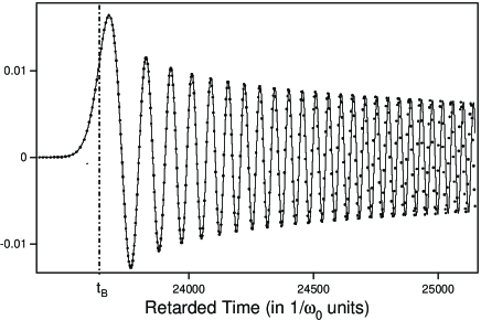
Figure 10: Brillouin precursor in the dispersion dominant limit. The solid line (bullets $\bullet$) is the exact numerical solution (the analytical solution). Parameters (in $\omega_{0}$ units): $\omega_{c}=0.836$, $\omega_{p}=1.11$, $\gamma=10^{-4}$ and $\xi=2.95\times 10^{4}$, leading to $\omega_{0}t_{B}\approx 2.3641\times 10^{4}$, $b\approx 0.0257\omega_{0}$ and $\beta\approx 0.252\omega_{0}$. The carrier frequency $\omega_{c}$ is at the lower boundary of the opacity region [$\alpha\left(\omega_{c}\right)z\approx 20$ ].

Fig.10 shows an example of Brillouin precursor obtained in such conditions ($\gamma/b\approx 3.9\times 10^{-3}$). It is worth emphasizing that, since $b\varpropto z^{-1/3}$, the condition $\gamma/b\ll 1$ requires that the propagation distance is not too large. On the other hand, it should be large enough for the inequality of Eq.(35) to be satisfied for a time larger or at least comparable to the half-maximum duration of the precursor. In fact, the most severe restriction originates in the condition $\omega_{0}\left(t-t_{B}\right)\leq\left(\omega_{0}/b\right)^{9/5}$ associated with the dispersion correction. When $\gamma\ll b$, we easily deduce from the asymptotic form of the Airy function that the half-maximum of the precursor will be attained for $\omega_{0}\left(t-t_{B}\right)\approx 20\left(\omega_{0}/b\right)$. The precursor will thus be well reproduced by the expression $e_{B}(z,t)\approx\left(b/\omega_{c}\right)Ai\left[-b\left(t-t_{B}\right)\right]$ beyond its half-maximum amplitude if $\gamma\ll b$ and if $\left(\omega_{0}/b\right)^{4/5}>20$, that is if $b/\omega_{0}<0.024$. The latter condition is approximately met Fig.10 for which $b/\omega_{0}=0.026$. As expected, the maximum amplitude of the precursor is $a_{B}\approx 0.536\left(b/\omega_{c}\right)\approx 0.0165$ , with $\exp\left(-2\gamma\left(t-t_{B}\right)/3\right)\approx 0.997$ at the corresponding time.

VI PROPAGATION OF PULSES WITH A SQUARE OR GAUSSIAN ENVELOPE

Up to now, in the spirit of the pioneering work of Sommerfeld and Brillouin, we have considered incident fields of infinite duration. In actual or even numerical experiments, this duration is naturally finite. As a matter of fact the simulations made to corroborate our previous analytical calculations were made by using a square-wave modulation (eventually suitably filtered) and choosing a square duration long enough to avoid that the precursors generated by the rise and the fall of the square overlap. On the contrary, we consider in this section the case where the duration of the incident field is small compared to the time-delay $t_{B}$ separating the Brillouin precursor from the Sommerfeld precursor and does not exceed few periods of the carrier. We will restrict the analysis to the Brillouin precursor. Indeed the Sommerfeld precursor, if it exists, is generally much smaller and will be often filtered out by rise-time effects, to which the Brillouin precursor is much less sensitive.

VI.1 Square pulse

We consider first a square-modulated incident field $\left[\mathrm{u}_{H}(t)-\mathrm{u}_{H}(t-T)\right]\sin\left(\omega_{c}t\right)$. Of particular interest is the case where the square duration is an integer $n$ of half-periods of the carrier, that is $T=nT_{c}/2=n\pi/\omega_{c}$. The incident field can then be rewritten as $e(0,t)=\mathrm{u}_{H}(t)\sin\left(\omega_{c}t\right)-\left(-1\right)^{n}\mathrm{u}_{H}(t-T)\sin\left[\omega_{c}\left(t-T\right)\right]$ and the transmitted field reads as $e^{\prime}(z,t)=e(z,t)-\left(-1\right)^{n}e(z,t-T)$ where $e(z,t)$ designates the transmitted field when only the incident field $\mathrm{u}_{H}(t)\sin\left(\omega_{c}t\right)$ is on. This equation applies to the whole field and in particular to the Brillouin precursor to yield:

$$e_{B}^{\prime}(z,t)=e_{B}(z,t)-\left(-1\right)^{n}e_{B}(z,t-T),$$ (37)

where $e_{B}(z,t)$ is given by Eq.(26) or Eq.(34), depending on the system and the parameters considered. The two components of $e_{B}^{\prime}$ are of opposite (same) sign when $n$ is even (odd) and are well separated when it is large enough, so that $T$ significantly exceeds the duration of the elementary precursor. On the other hand, $e_{B}(z,t)$ evolving slowly at the scale of $T_{c}$, the two components overlap and interfere if $n$ is small. When $n=2$ ($T=T_{c}$) as considered in ou05 ; ou90 , the two components interfere nearly destructively to give a precursor $e_{B}^{\prime}(z,t)\approx T_{c}\dot{e}_{B}(z,t-T_{c}/2)$. The case where $n$ is odd and, in particular, where $n=1$ ($T=T_{c}/2$) is much more favorable. Indeed the two precursors then interfere constructively to yield a precursor $e_{B}^{\prime}(z,t)\approx 2e_{B}(z,t-T_{c}/4)$ whose amplitude is twice that obtained with a step modulation. This result is not really a surprise since the pulse area is itself twice that of $\mathrm{u}_{H}(t)\sin\left(\omega_{c}t\right)$ . On the contrary the pulse area equals zero when $n$ is even. The previous results are illustrated Fig.11 that shows the Brillouin precursors obtained for $n=1,2$ for a Lorentz medium when attenuation and dispersion comparably contribute to the formation of the Brillouin precursor (simple asymptotic limit).

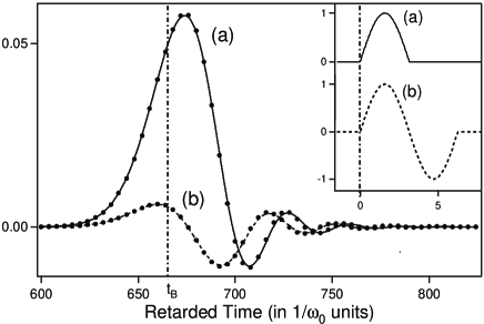
Figure 11: Comparison of the Brillouin precursors $e^{\prime}_{B}(z,t)$ generated by an incident square-modulated field of duration (a) $T=T_{c}/2$ and (b) $T=T_{c}$ . The parameters are those of Fig.8. The solid and dashed lines are the exact numerical solutions, indiscernible from the analytical solutions given by Eq.(37). The bullets are the approximate solutions (a) $2e_{B}(z,t-T_{c}/4)$ and (b) $T_{c}\dot{e}_{B}(z,t-T_{c}/2$ . As expected the precursor amplitude for $T=T_{c}/2$ is twice that attained with a step-modulated field (see Fig.8) whereas that attained for $T=T_{c}$ is much smaller. Inset: corresponding incident fields.

When the detection of the Brillouin precursor is not time-resolved an important parameter is the integrated “energy” $W_{B}(z)=\intop_{-\infty}^{+\infty}\left|e^{\prime}_{B}(z,t)\right|^{2}dt$ choi04 ; lu09 . Thanks to the Parseval-Plancherel theorem pap87 , it can be written as

$$W_{B}(z)=\frac{1}{2\pi}\intop_{-\infty}^{+\infty}\left|H_{B}(z,\omega)\right|^{2}\left|E(0,\omega)\right|^{2}d\omega.$$ (38)

In this expression all phases are eliminated and $\left|H_{B}(z,\omega)\right|^{2}$ is reduced to $\exp\left(-4\gamma\omega^{2}/3b^{3}\right)=\exp\left(-\omega^{2}/2\beta^{2}\right)$ in both strict and simple asymptotic cases. For $T=T_{c}/2$, $\left|H_{B}(z,\omega)E(0,\omega)\right|^{2}\approx\left(4/\omega_{c}^{2}\right)\exp\left(-\omega^{2}/2\beta^{2}\right)$ and we get an energy $W_{B}(z)=2^{3/2}\pi^{-1/2}\beta/\omega_{c}^{2}$ which slowly decays with the propagation distance (as $1/\sqrt{z}$). On the other hand, for $T=T_{c}$, $\left|H_{B}(z,\omega)E(0,\omega)\right|^{2}\approx\left(2\pi\omega/\omega_{c}^{2}\right)^{2}\exp\left(-\omega^{2}/2\beta^{2}\right)$ and $W_{B}(z)=(2\pi)^{3/2}\beta^{3}/\omega_{c}^{4}$. As expected, $W_{B}(z)$ then decays very rapidly with the propagation distance (as $z^{-3/2}$). As already mentioned, the previous expressions of the energy are valid regardless of the relative contributions of the absorption and the dispersion to the formation of the precursor. For the Debye medium and the Lorentz medium in the dominant-attenuation limit, it is besides possible to derive from Eq.(37) and Eq.(26) explicit expressions of the maximum amplitude $a_{B}^{\prime}(z)$ of the precursor $e_{B}^{\prime}(z,t)$. We find that this amplitude, equal to $2\beta/\left(\omega_{c}\sqrt{\pi}\right)\approx 1.1\left(\beta/\omega_{c}\right)\propto 1/\sqrt{z}$ when $T=T_{c}/2$, falls down to $2\sqrt{2\pi/\mathrm{e}}\left(\beta/\omega_{c}\right)^{2}\approx 3.0\left(\beta/\omega_{c}\right)^{2}\propto 1/z$ when $T=T_{c}$.

VI.2 Gaussian pulse

The Gaussian pulses are probably the sole smooth pulses for which it is possible to obtain exact analytic expressions of the Brillouin precursor, both in the strict and simple asymptotic limit. Non-chirped incident fields of the form $\mathrm{e}^{-t^{2}/T^{2}}\cos\left(\omega_{c}t\right)$ and $\mathrm{e}^{-t^{2}/T^{2}}\sin\left(\omega_{c}t\right)$ have been respectively considered by Oughstun and Balictsis in ou96 and by Ni and Alfano in ni06 . When the pulses are linearly chirped, it is convenient to consider them as the real and imaginary part of $\widetilde{e}(0,t)=\exp\left(i\omega_{c}t-t^{2}/T^{2}+i\chi^{2}t^{2}\right)$ where $\chi^{2}$ is the chirping parameter. The Fourier transform of $\widetilde{e}(0,t)$ and of the corresponding transmitted field $\widetilde{e}_{B}(z,t)$ simply read as $\widetilde{E}(0,\omega)=\widetilde{T}\sqrt{\pi}\exp\left[-\left(\omega-\omega_{c}\right)^{2}\widetilde{T}^{2}/4\right]$ and

$$\widetilde{E}_{B}(z,\omega)=\widetilde{\mathcal{A}}H_{B}(z,\omega)\exp\left(-\omega^{2}\widetilde{T}^{2}/4+\omega\omega_{c}\widetilde{T}^{2}/2\right).$$ (39)

In these expressions $\widetilde{T}=T/\sqrt{1-i\chi^{2}T^{2}}$ and $\widetilde{\mathcal{A}}=\widetilde{T}\sqrt{\pi}\exp\left(-\omega_{c}^{2}\widetilde{T}^{2}/4\right)$ may be respectively seen as the (complex) duration and area of the pulse $\widetilde{e}(0,t)$. In the strict asymptotic limit [see Eq.(24)], we get

$$\widetilde{E}_{B}(z,\omega)=\widetilde{\mathcal{A}}\exp\left[-\frac{\omega}{4}^{2}\left(\frac{1}{\beta^{2}}+\widetilde{T}^{2}\right)+\omega\frac{\omega_{c}\widetilde{T}^{2}}{2}\right],$$ (40)

and $\widetilde{e}_{B}(z,t)$, inverse Fourier transform of $\widetilde{E}_{B}(z,\omega)$, reads as

$$\widetilde{e}_{B}(z,t)=\frac{\widetilde{\mathcal{A}}\beta}{\sqrt{\pi\left(1+\beta^{2}\widetilde{T}^{2}\right)}}\\ \times\exp\left[-\frac{\beta^{2}\left(t^{\prime}-i\omega_{c}\widetilde{T}^{2}/2\right)}{1+\beta^{2}\widetilde{T}^{2}}\right]$$ (41)

where $t^{\prime}=t-t_{B}$. In the simple asymptotic limit (see Sec. V), Eq.(31) and Eq.(39) yield

$$\widetilde{E}_{B}(z,\omega)=\widetilde{\mathcal{A}}\exp\left[-i\omega\left(t_{B}+\frac{i\omega_{c}\widetilde{T}^{2}}{2}\right)\right]\\ \times\exp\left[-\omega^{2}\left(\frac{2\gamma}{3b^{3}}+\frac{\widetilde{T}^{2}}{4}\right)-i\omega^{3}\left(\frac{1}{3\eta b^{3}}\right)\right]$$ (42)

This equation is easily transformed in an equation similar to Eq.(32). By this way, we find

$$\widetilde{e}_{B}(z,t)=\widetilde{\mathcal{A}}\>\widetilde{B}\>\mathrm{Ai}\left(-\eta^{1/3}b\>\widetilde{t}\right)\exp\left(-\frac{2}{3}\eta\widetilde{\gamma}\>\widetilde{t}\right),$$ (43)

where $\widetilde{\gamma}=\gamma+3b^{3}\widetilde{T}^{2}/8$, $\widetilde{B}=\eta^{1/3}b\>\exp\left[-(\eta^{2}/3)\left(2\widetilde{\gamma}/3b\right)^{3}\right]$ and $\widetilde{t}=t-t_{B}-4\eta\widetilde{\gamma}^{2}/9b^{3}-i\omega_{c}\widetilde{T}^{2}/2$. Finally the precursors generated by the incident fields $\mathrm{e}^{-t^{2}/T^{2}}\cos\left(\omega_{c}t+\chi^{2}t^{2}\right)$ and $\mathrm{e}^{-t^{2}/T^{2}}\sin\left(\omega_{c}t+\chi^{2}t^{2}\right)$ respectively read as $e_{cos}(z,t)=\Re\left[\widetilde{e}_{B}(z,t)\right]$ and $e_{sin}(z,t)=\Im\left[\widetilde{e}_{B}(z,t)\right]$. Eq.(41), Eq.(43) and the derived expressions of $e_{cos}(z,t)$ and $e_{sin}(z,t)$ hold whatever the duration of the incident pulse may be. However, as shown below, the amplitude of the Brillouin precursor will be only significant when this duration does not exceed a few periods of the carrier. In the Fourier transform $H_{B}(z,\omega)\widetilde{E}(0,\omega)$ of the transmitted field, $H_{B}(z,\omega)$ is then again much narrower than $\widetilde{E}(0,\omega)$, which may be approximated by its first order expansion in powers of $\omega$. We get so $\widetilde{E}_{B}(z,\omega)\approx\widetilde{\mathcal{A}}\left(1+\omega\omega_{c}\widetilde{T}^{2}/2\right)H_{B}(z,\omega)$ and finally

$$\widetilde{e}_{B}(z,t)\approx\widetilde{\mathcal{A}}\left[h_{B}(z,t)-\left(i\omega_{c}\widetilde{T}^{2}/2\right)\dot{h}_{B}(z,t)\right].$$ (44)

When there is no chirping, $\widetilde{T}$ and $\widetilde{\mathcal{A}}$ are real, with $\widetilde{T}=T$ and $\widetilde{\mathcal{A}}=\mathcal{A}=T\sqrt{\pi}\exp\left[-\omega_{c}^{2}T^{2}/4\right]$. Eq.(44) then leads to

$$e_{cos}(z,t)\approx\mathcal{A}\>h_{B}(z,t)\\ =T\sqrt{\pi}\exp\left[-\frac{\omega_{c}^{2}T^{2}}{4}\right]\>h_{B}(z,t)$$ (45)

$$e_{sin}(z,t)\approx-\frac{\mathcal{A}\omega_{c}T^{2}}{2}\>\dot{h}_{B}(z,t)=-\frac{\omega_{c}T^{2}}{2}\>\dot{e}_{cos}(z,t).$$ (46)

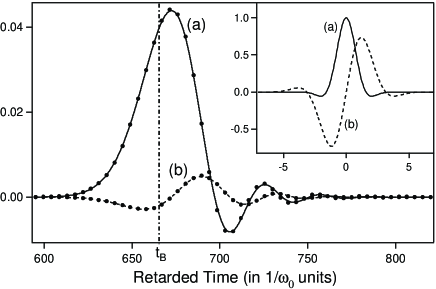
Figure 12: Brillouin precursors generated by the incident fields of Gaussian envelope (a) $\mathrm{e}^{-(t/T)^{2}}\mathrm{cos}(\omega_{c}t)$ with $T=\sqrt{2}/\omega_{c}$ and (b) $\mathrm{e}^{-(t/T)^{2}}\mathrm{sin}(\omega_{c}t)$ with $T=\sqrt{6}/\omega_{c}$. The parameters are those of Fig.8. In both cases, the pulse duration has been chosen in order to maximize the precursor amplitude (see text). The solid and dashed lines are the exact numerical solutions whereas the bullets are the analytical solutions obtained in the short pulse approximation [Eq.(45) and Eq.(46)], indiscernible from those obtained without approximation [Eq.(43)]. Inset: corresponding incident fields. Numerical calculations shows that the Sommerfeld precursors generated by these fields have negligible amplitudes, respectively (a) $5.6\times 10^{-7}$ and (b) $1.15\times 10^{-10}$.

As illustrated Fig.12, obtained in the simple asymptotic limit, these approximate analytic solutions perfectly fit the exact numerical solution. It is easily deduced from Eq.(45) [Eq.(46)] that the amplitude of the precursor $e_{cos}(z,t)$ [$e_{sin}(z,t)$] is maximum for a pulse duration $T=T_{m}=\sqrt{2}/\omega_{c}$ [ $\sqrt{6}/\omega_{c}$]. The energy of the precursors can be obtained by the method already used in the case of a square modulation. We get so $W_{B}\approx\left(\pi/2\right)^{1/2}\left(\beta T^{2}e^{-\omega_{c}^{2}T^{2}/2}\right)\propto 1/\sqrt{z}$ for $e(0,t)=\mathrm{e}^{-t^{2}/T^{2}}\cos\left(\omega_{c}t\right)$ and $W_{B}\approx\left(\pi/32\right)^{1/2}\left(\beta^{3}\omega_{c}^{2}T^{6}e^{-\omega_{c}^{2}T^{2}/2}\right)\propto z^{-3/2}$ for $e(0,t)=\mathrm{e}^{-t^{2}/T^{2}}\sin\left(\omega_{c}t\right)$. In fact the scaling laws in $z^{-1/2}$ or $z^{-3/2}$ are general and hold for every short incident pulse. In all cases, the transmitted pulse is indeed proportional to $h_{B}(z,t)$ when $E(0,0)=\mathcal{A}\neq 0$ or to $\dot{h}_{B}(z,t)$ when $\mathcal{A}=0$, the proportionality coefficient depending only on the characteristics of the incident pulse and not on the propagation distance. For Gaussian incident pulses and, more generally, for smooth pulses, the amplitude and the energy of the Brillouin precursor rapidly decreases with the pulse duration. For example, the amplitude of the Brillouin precursor generated by the incident field $\mathrm{e}^{-t^{2}/T^{2}}\cos\left(\omega_{c}t\right)$ is reduced by a factor exceeding $400$ when $T$ is taken four times larger than its optimum value $\sqrt{2}/\omega_{c}$ [see Eq.(45)]. This reduction of amplitude can however be compensated by using chirped pulses. When the pulse duration remains small enough, Eq.(44) holds and the Brillouin precursor generated by the incident field $\mathrm{e}^{-t^{2}/T^{2}}\cos\left(\omega_{c}t+\chi^{2}T^{2}\right)$ reads as

$$e_{B}(z,t)\approx h_{B}(z,t)\>\Re\left(\widetilde{\mathcal{A}}\right)\\ -\dot{h}_{B}(z,t)\>\Re\left(i\omega_{c}\widetilde{\mathcal{A}}\widetilde{T}^{2}/2\right).$$ (47)

Anticipating that the second term of this equation is small compared to the first one, we easily get the approximate expression

$$e_{B}(z,t)\approx\mathcal{A}\>h_{B}\left[z,t"-\Re\left(i\omega_{c}\widetilde{\mathcal{A}}\widetilde{T}^{2}/2\mathcal{A}\right)\right],$$ (48)

where $\mathcal{A}=\Re\mathcal{\left(\widetilde{A}\right)}$ is the area of the incident pulse. This result differs from that obtained without chirping [see Eq.(45)] by a extra time-delay $\Re\left(i\omega_{c}\widetilde{\mathcal{A}}\widetilde{T}^{2}/2\mathcal{A}\right)$ and, moreover, by the pulse area $\mathcal{A}$ that may be considerably larger than that attained when the pulse is not chirped.

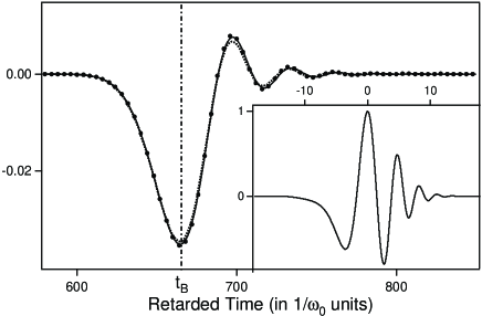
Figure 13: Brillouin precursor generated by a chirped incident pulse $e^{-\left(t/T\right)^{2}}\cos\left(\omega_{c}t+\chi^{2}t^{2}\right)$, with $T=4\sqrt{2}/\omega_{c}$ and $\chi=\omega_{c}/4$ . The other parameters are as those of Fig.8 and Fig.12. The solid line, the bullets and the dashed line respectively are the exact numerical solution, the analytic solution derived from Eq.(43) and the approximate analytic solution of Eq.(48), obtained in the short pulse approximation. Inset: incident pulse. The corresponding Sommerfeld precursor has fully negligible amplitude ($9\times 10^{-11}$ !).

Fig.13 shows the result obtained for a pulse duration $T=4\sqrt{2}/\omega_{c}$. In order to maximize the precursor amplitude, we have chosen for the chirping the value $\chi=\omega_{c}/4$ for which the function $\mathcal{A}(\chi)$ reaches its first extremum (negative minimum). For these parameters, $\Re\left(i\mathcal{A}\widetilde{T}^{2}/2\mathcal{A}\right)$ is also negative (time advancement). We remark that, despite the numerous approximations having led to Eq.(48), it provides a very good approximation of the exact result.

VII Conclusion

We have analytically studied the propagation of light pulses in a dense Lorentz medium at distances $z$ so large that the medium is opaque in a broad spectral region and the Sommerfeld and Brillouin precursors are far apart from each other.

Assuming that the carrier frequency $\omega_{c}$ lies in the opacity region (below, inside or beyond the anomalous dispersion region), we have shown that the Sommerfeld precursor has a shape independent of $\omega_{c}$ and that it is entirely determined by the order $p$ and the importance $d_{p}$ of the initial discontinuity of the incident field, regardless of its subsequent evolution. When the incident field is discontinuous ($p=0$), its amplitude is independent of $z$ and $\omega_{c}$ . For $p>0$, this amplitude is proportional to $\omega_{c}z^{-(2p+1)/4}$ and rapidly decreases with the rise time of the incident field. These results, exact in the strict asymptotic limit where $z\rightarrow\infty$, provide excellent approximations for the propagation distance considered by Brillouin and remain good approximations even when $z$ is 1 000 times shorter.

In the strict asymptotic limit, the formation of the Brillouin precursor is uniquely determined by the frequency dependence of the medium attenuation. When $\omega_{c}$ lies in the opacity region, we have shown that the Brillouin precursor is a Gaussian of amplitude $a_{B}\varpropto 1/\left(\omega_{c}\sqrt{z}\right)$ or a Gaussian-derivative of amplitude $a_{B}\varpropto 1/\left(\omega_{c}^{2}z\right)$, depending whether the area of the incident field differs or not from zero. We have also determined the transmitted field when $\omega_{c}$ is outside the opacity region, evidencing the “pollution” of the Brillouin precursor by the field that is then transmitted at $\omega_{c}$ (Fig.7).

In a simple asymptotic limit, both attenuation and group delay dispersion contribute to the formation of the Brillouin precursor. We have established in this case an expression of the Brillouin precursor containing as particular cases the previous one (dominant-attenuation limit) and that obtained by Brillouin by means of the stationary phase method (dominant-dispersion limit).

We have finally obtained exact analytical expressions of the Brillouin precursors originated by pulses of square or Gaussian envelope. We have in particular determined the pulse parameters optimizing the precursor amplitude and demonstrated that the energy of the precursor decreases with the propagation distance as slowly as $z^{-1/2}$ when the area of the incident field differs from zero but as rapidly as $z^{-3/2}$ in the contrary case. We have also shown that, for a given duration, the precursor amplitude can be greatly enhanced by using frequency-chirped pulses.

Our explicit analytic expressions of the precursors contrast by their simplicity from those currently derived by the uniform saddle point methods. The complexity of the latter ou09 is often such that it is difficult and sometimes impossible to retrieve from them our asymptotic forms. On the other hand, it should be kept in mind that our results only hold in the limit where the medium is opaque in a spectral region whose width is much larger than the resonance frequency. We however remark that they provide a not too bad reproduction of the Sommerfeld and Brillouin precursors even when this width is of the order of the resonance frequency (Fig.9). We finally mention that the study of the precursors is greatly simplified when the complex index of the medium is such that $\lvert\widetilde{n}(\omega)-1\rvert\ll 1$ $\forall\omega$ bm11 . As in the study of the quasi-resonant precursors bm09 , the equation giving the saddle points can then be reduced to a biquadratic form and the saddle point method is expected to provide simple solutions even when the Sommerfeld and Brillouin precursors partially overlap. This work is in progress.

References

- (1) A. Sommerfeld, Physikalische Zeitschrift 23, 841 (1907) [in German].
- (2) A. Sommerfeld, Ann. Phys. (Leipzig) 44, 177 (1914) [in German].
- (3) L. Brillouin, Ann. Phys. (Leipzig) 44, 203 (1914) [in German].
- (4) L. Brillouin, in Comptes Rendus du Congrès International d’Electricité, Paris 1932 (Gauthier-Villars 1933), Vol.2, pp 739-788 [in French].
- (5) L. Brillouin, Wave Propagation and Group Velocity (Academic Press, New York 1960), Authorized translations in English of som14 ; bri14 ; bri32 can be found in this book, respectively in Ch. II, Ch. III, Ch. IV and Ch. V.
- (6) J.A. Stratton, Electromagnetic Theory (McGraw-Hill, New York 1941).
- (7) J. D. Jackson, Classical Electrodynamics, 2nd ed. (Wiley, New York 1975).
- (8) R.A. Handelsman and N. Bleistein, Arch. Rat. Mech. Anal. 35, 267 (1969).
- (9) K.E. Oughstun and G.C. Sherman, Proceedings of the URSI Symposium on Electromagnetic Wave Theory (Stanford University, 1977), pp 34-36.
- (10) V.A. Vasilev, M.Y. Kelbert, I.A. Sazonov and I.A. Chaban, Opt. Spectrosk. 64, 862 (1988) [Opt. Spectrosc. 64, 513 (1988)].
- (11) K.E. Oughstun and G.C. Sherman, J. Opt. Soc. Am. A 6, 1394 (1989).
- (12) A. Karlsson and S. Rike, J. Opt. Soc. Am. A 15, 487 (1998).
- (13) K.E. Oughstun, Electromagnetic and Optical Pulse Propagation 2 : Temporal Pulse Dynamics in Dispersive Attenuative Media (Springer, New York, 2009).
- (14) A. Ciarkowski, J. Tech. Phys. 43, 187 (2002).
- (15) A. Ciarkowski, J. Tech. Phys. 44, 181 (2003).
- (16) B. Macke and B. Ségard, J. Opt. Soc. Am. B 28, 450 (2011).
- (17) A. Ciarkowski, International Journal of Electronics and Telecommunications (JET) 57, 251 (2011).
- (18) S.H. Choi and U. Österberg, Phys. Rev. Lett. 92, 193903 (2004).
- (19) R.R. Alfano, J.L. Birman, X. Ni, M. Alrubaiee, and B.B. Das, Phys. Rev. Lett. 94, 239401 (2005).
- (20) T.M. Roberts, Phys. Rev. Lett. 93, 269401 (2004).
- (21) D. Lukofsky, J. Bessette, H. Jeong, E. Garmire, and U. Österberg, J. Mod. Opt. 56, 1083 (2009).
- (22) L.M. Naveira, B.D. Strycker, J. Wang, G.O. Ariunbold, A.V. Sokolov, and G.W. Kattawar, Appl. Opt. 48, 1828 (2009).
- (23) M.M. Springer, W.Yang, A.A. Kolomenski, H.A. Schuessler, J. Strohaber, G.W. Kattawar, and A.V. Sokolov, Phys. Rev. A 83, 043817 (2011).
- (24) E. Varoquaux, G. A. Williams, and O. Avenel, Phys. Rev. B 34, 7617(1986).
- (25) J. Aaviksoo, J. Kuhl, and K. Ploog, Phys. Rev. A 44, R5353 (1991).
- (26) B. Ségard, J. Zemmouri, and B. Macke, Europhys. Lett. 4, 47 (1987). See Fig.2 in this reference. Note that the experiment was performed at a millimeter wavelength instead of in the optical domain and was not analyzed in terms of precursors.
- (27) H. Jeong, A. M. C. Dawes, and D. J. Gauthier, Phys. Rev. Lett., 96, 143901 (2006). In this experiment, the optical thickness of the medium for the amplitude was only , not sufficient to observe the characteristic beat between Sommerfeld and Brillouin precursors. See: B. Macke and B. Ségard, e-print arXiv:physics/0605039
- (28) Dong Wei, J.F. Chen, M.M.T. Loy, G.K.L. Wong, and S. Du, Phys. Rev. Lett. 103, 093602 (2009).
- (29) See bri60 , pp. 55-57 and 127-128.
- (30) We use the definitions, sign conventions and results of the linear system theory. See for example A.Papoulis, The Fourier Integral and its Applications (Mc Graw Hill, New York 1987).
- (31) Keep in mind that we use a retarded time picture where the time is the real time minus the luminal propagation time .
- (32) Handbook of Mathematical functions, edited by M. Abramowitz and I. A. Stegun (Dover, New York, 1972).
- (33) As usual, we consider that the zero-order derivative of a function is the function itself.
- (34) K.E Oughstun, J. Opt. Soc. Am. A 12, 1715 (1995).
- (35) N. S. Bukhman, Quantum Electron. 34, 299 (2004).
- (36) B. Macke and B. Ségard, Phys. Rev. A 73, 043802 (2006).
- (37) J.R. Klauder, IEE Proc. Rad. Sonar Navig. 152, 23 (2005) and e-print arXiv:math/0402410.
- (38) D. C. Stoudt, F. E. Peterkin, and B. J. Hankla, Transient RF and Microwave Pulse Propagation in a Debye Medium (Water), NSWC Report JPOSTC-CRF-005-03 (Dalgreen, 2001).
- (39) J. Garnier and K. Solna, Waves in Random and Complex Media 20, 122 (2010).
- (40) K. E. Oughstun, IEEE Trans. Antennas Propag. 53, 1582 (2005).
- (41) M. Pieraccini, A. Bicci, D. Mecatti, G. Macaluso, and C. Atzeni, IEEE Trans. Antennas Propag. 57, 3612 (2009).
- (42) M. Dawood, H. R. Mohammed, and A. V. Alejos, Electron. Lett. 46, 1645 (2010).
- (43) N. Cartwright, IEEE Trans. Antennas Propag. 59, 1571 (2011).
- (44) Note that the Airy function used by Brillouin differs from that currently used , with . Peak amplitudes of and are respectively and .
- (45) K. E. Oughstun and G. C. Sherman, Phys. Rev. A 41, 6090 (1990).
- (46) K. E. Oughstun and C. M. Balictsis, Phys. Rev. Lett. 77, 2210 (1996).
- (47) X. Ni and R. R. Alfano, Optics Express 14, 4188 (2006).
- (48) B. Macke and B. Ségard, Phys. Rev. A 80, 011803(R) (2009).