A Bayesian measurement error model for two-channel cell-based RNAi data with replicates

Abstract

RNA interference (RNAi) is an endogenous cellular process in which small double-stranded RNAs lead to the destruction of mRNAs with complementary nucleoside sequence. With the production of RNAi libraries, large-scale RNAi screening in human cells can be conducted to identify unknown genes involved in a biological pathway. One challenge researchers face is how to deal with the multiple testing issue and the related false positive rate (FDR) and false negative rate (FNR). This paper proposes a Bayesian hierarchical measurement error model for the analysis of data from a two-channel RNAi high-throughput experiment with replicates, in which both the activity of a particular biological pathway and cell viability are monitored and the goal is to identify short hair-pin RNAs (shRNAs) that affect the pathway activity without affecting cell activity. Simulation studies demonstrate the flexibility and robustness of the Bayesian method and the benefits of having replicates in the experiment. This method is illustrated through analyzing the data from a RNAi high-throughput screening that searches for cellular factors affecting HCV replication without affecting cell viability; comparisons of the results from this HCV study and some of those reported in the literature are included.

abstract width 300pt

T1Supported in part by NRPGM Grants NSC 95-3112-B001-019, NSC 96-3112-B001-003, NSC 96-3112-B001-012, NSC 97-3112-B001-001, NSC-98-3112-B-400-009 and NSC-98-3112-B-400-010.

, , , , , , , and

1 Introduction

1.1 RNA interference high-throughput screening and the motivating example

RNA interference (RNAi) is a conserved biological pathway by which messenger RNAs are targeted for degradation by double stranded RNA of identical sequence and, thus, it silences gene expression on the level of individual transcripts [Chapman and Carrington (2007), Fire et al. (1998)]. For example, in mammalian cells, small interfering RNAs (siRNAs) are effective in silencing target mRNAs [Echeverri et al. (2006), Elbashir et al. (2001), Hannon and Zamore (2003)]. Initially, it was used to knockdown the function of individual genes of interest; with the production of RNAi libraries, it is possible for the current technology to silence most of the genes in the genome and conduct genome-wide loss-of-function screening so as to identify previously unknown genes involved in a biological pathway; it provides a systematic analysis of the genome. The purpose of RNAi high-throughput screening (HTS) is to identify a set of siRNAs affecting the cellular phenotype of interest; in the HTS literature, this is referred to as hit selection. For example, RNAi technology has opened up the field of genomic scale cell-based screening to the study of viral-host interactions [Cherry (2009)] and several RNAi HTS have been conducted to identify cellular factors required for various viral infections.

As Boutros and Ahringer (2008) and Echeverri et al. (2006) pointed out, while RNAi HTS is promising and has generated various significant technical advances and scientific findings, there are still challenges regarding high-throughput assay development and data analysis. In particular, Cherry (2009) and Tai et al. (2009) remarked that in the studies of viral-host interactions, while RNAi HTS has led to the discovery of hundreds of new factors and increased our knowledge of the host factors that impact viral infection and highlighted the cellular pathways at play, there is a surprising lack of concordance between the results of seemingly similar screens. Among issues to be considered when comparing these studies, one recognizes the need to standardize the statistics methods and to address the false positive and false negative rates inherent to high-throughput siRNA screens.

We note that RNAi HTS refers to a wide range of different experiments. To determine the assay appropriate for the biological process to be investigated and to choose or develop statistical methods suitable for data resulting from the experiments are of great importance; see Boutros and Ahringer (2008). More specifically, this paper treats the simple situation that uses cell-based homogeneous assay, in which the phenotypes of many cells are averaged across each well in a microtitre plate. In particular, we are interested in data generated from a two-channel cell-based RNAi HTS experiment where the phenotype of a pathway-specific reporter gene and that of a constitutive reporter are measured; such experimental setups are typically used in screens for signaling pathway components; see page R66.5 of Boutros, Bras and Huber (2006). Typical examples include RNAi HTS experiments designed for the identification of cellular factors required for viral infections, in which cell viability is measured and used to account for the effect of unequal cell numbers in different wells on the measurements of virus RNA replication.

This experimental setup makes it possible to distinguish changes in the readout caused by depletion of the specific pathway components and changes incurred by the changes in the overall cell number. Based on the plot for a two-channel RNAi HTS experiment, Boutros, Bras and Huber (2006) suggest, for a given siRNA, the ratio of the log of the readout of the specific pathway to the log of the overall cell number is used as a summary of the effect of the siRNA on the specific pathway. In the analysis of data from RNAi HTS to identify host factors involved in HIV-1 replication, Börner et al. (2010) also carried out log transformation of the raw data, including both the measurement of the pathway activity and the cell count in each well, and applied a robust locally weighted regression [Cleveland (1979)] to smooth the scatterplot of the log transformed data. In a sense, this seems to be an extension and improvement of the suggestion of Boutros, Bras and Huber (2006).

To make a more systematic use of the data, we propose a Bayesian regression model that treats cell viability as a covariate and the specific pathway activity measurement as the response variable so that the pathway activity change can be studied in terms of the regression coefficient and the issues of false positive and false negative rates can be handled in the Bayesian framework.

Statistical methods for cell-based RNAi HTS have been introduced and reviewed by Boutros, Bras and Huber (2006), Zhang et al. (2006), Zhang et al. (2008), Malo et al. (2006) and Birmingham et al. (2009), among others. Most of them deal with one-channel screening and use descriptive quantities like fold change or simple statistics like $Z$-score or $t$-test to identify a set of siRNAs that inhibit or activate defined cellular phenotypes. The only exceptions are Zhang et al. (2008), who proposed a Bayesian method for one-channel screening experiments to handle false positive and false negative rates, and Boutros, Bras and Huber (2006), who included some discussions on two-channel experiments.

Another feature of our experiment is that for each siRNA, the experiment is replicated in $2J$ wells, where $J$ of them measure cell viability and the other $J$ measure the specific pathway activity. We note that Tai et al. (2009) is an example of two-channel RNAi HTS with $J=2$ replicates, with pooled siRNAs though, and that the dual channel experiment mentioned in Boutros, Bras and Huber (2006) also has $J=2$ replicates. Our method will make use of these replicates.

Our method is motivated by the following RNAi HTS that searches for the cellular factors that affect HCV replication without affecting cell viability, referred to as the HCV study in this paper. HCV (hepatitis C virus) is a small, enveloped, positive-sense single-stranded RNA virus of the family Flaviviridae and the cause of hepatitis C in humans; see Ryan and Ray (2004). It is estimated that hepatitis C has infected nearly $200$ million people worldwide, and is now infecting $3$ to $4$ million people per year (WHO, see the URL below). It is currently a leading cause of cirrhosis, a common cause of hepatocellular carcinoma. As a result of these conditions, it is the leading reason for liver transplantation in, for example, the United States (NIDA, see the URL below).

The experiment is carried out as follows. A Huh-7-derived HCV-Luc cell line that contains the genome of the HCV and harbors the luciferase gene as a reporter is employed as a cell-based system for RNA interference screening. We have shown that luciferase activity correlates well with the HCV replication (data not shown). The HCV-Luc cells are transduced by the lentiviruses each carrying specific short-hairpin RNA (shRNA) and puromycin-resistant gene. In these circumatances, lentivirus-transduced cells survive under puromycin selection. HCV RNA replication in the well can now be measured in terms of the expression of luciferase in HCV-Luc and cell viability in the well can be measured by a colorimetric method which monitors the level of dehydrogenase in viable cells.

A VSV-G pseudotyped lentivirus-based RNAi library targeting a whole panel of human kinases and phosphatases was employed [Moffat et al. (2006)] in this study. This library includes $6\mbox{,}390$ shRNAs designed to target 1,187 genes. HCV-Luc cells are seeded in 96-well plates and each well is transduced with one of these $6\mbox{,}390$ shRNAs. There are in total $71$ plates and each plate has about $6$ wells for the controls. There are three types of controls: spike negative (SN), no transduction no puromycin selection (NTNP), and no tranduction with puromycin selection (NTWP). In SN control wells, the nonhuman gene targeting shLacZ is used instead of the above-mentioned shRNAs; data from these wells serve as the RNAi machinery competition controls. In NTNP control wells, cells are not transduced by lentiviruses nor subjected to puromycin selection. In NTWP control wells, cells are not transduced by lentiviruses but subjected to puromycin selection. There are in total $142$ SN wells with most plates having $2$ SN wells in each plate, $217$ NTNP wells with most plates having $3$ NTNP wells in each plate and $67$ NTWP wells with most plates having one NTWP well in each plate. It is believed that in both SN and NTNP wells, we should observe normal HCV RNA replication and in NTWP wells, we should observe little HCV RNA replication and minimal cell viability.

The experiment described in the previous two paragraphs is replicated four times in a plate-by-plate manner; specifically, for each plate, there are three replicated plates in the sense that wells at the same position in these four plates are transduced by the same shRNA. We call this platewise replication. Among these four plates, we use two of them to measure cell viability and the other two to report luciferase activity as a surrogate for HCV RNA replication assay.

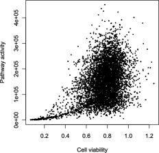
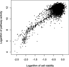
(a)	(b)

Figure 1: Plots for the HCV study data after preprocessing. There are in total $6\mbox{,}130$ data points with the $419$ controls excluded. (a) On the original measurement scale; (b) on the log transformed scale.

1.2 A log-linear measurement error model

Let $\tilde{x}_{ij}$ denote the measurement of the cell viability in the $j$th well of the $i$th shRNA. Let $\tilde{y}_{ij}$ denote the measurement of the pathway activity in the $(J+j)$th well of the $i$th shRNA. Here $i=1,\ldots,I$ and $j=1,\ldots,J$ with $J>1$. In practice, both $\tilde{x}_{ij}$ and $\tilde{y}_{ij}$ refer to the measurements undergone in certain data preprocessing steps so as to have reduced systematic bias. Figure 1 gives the data plot; Figure 1(a) is a plot of the data from the above HCV study with $\tilde{x}_{ij}$ and $\tilde{y}_{ij}$, respectively, the horizontal and vertical coordinates for $I=6\mbox{,}549$ and $j=1$; Figure 1(b) is the corresponding plot for $\log\tilde{x}_{ij}$ and $\log\tilde{y}_{ij}$. Visual examination of Figure 1(a), (b) suggests that a linear model on the logarithm transformed data is considered. In fact, the Additional data file 4 in Boutros, Bras and Huber (2006) also suggests the consideration of logarithm transformed data in a two-channel experiment based on their data. Another reason for this logarithm transformation is that based on Q–Q plots, both $\log\tilde{x}_{i1}-\log\tilde{x}_{i2}$ and $\log\tilde{y}_{i1}-\log\tilde{y}_{i2}$ are, respectively, much closer to normal distributions than $\tilde{x}_{i1}-\tilde{x}_{i2}$ and $\tilde{y}_{i1}-\tilde{y}_{i2}$. In fact, we found that logarithm transformation is very close to those suggested by the Box–Cox transformation [Box and Cox (1964)] technique.

Motivated by the above exploration, we assume that there exist $\mu_{i}$ and $\nu_{i}$ such that $\log(\tilde{x}_{i1})-\mu_{i}$ and $\log(\tilde{x}_{i2})-\mu_{i}$ are independent with mean zero and likewise $\log(\tilde{y}_{i1})-\nu_{i}$ and $\log(\tilde{y}_{i2})-\nu_{i}$ are also independent with mean zero.

We note that this formulation takes advantage of the replication in the experiment design and $e^{\mu_{i}}$ and $e^{\nu_{i}}$ represent, respectively, the expected cell viability and pathway activity when transduced by the $i$th shRNA. For the $i$th shRNA, denote by $\gamma_{i}=0$ if it incurs no change on the pathway activity, and by $\gamma_{i}=1$ if it does; in case $\gamma_{i}=1$, the magnitude of the change is represented by $\beta_{i}$. $\gamma_{i}$ is usually called the model index parameter. The plot in Figure 1(b) suggests a linear relation between $\nu_{i}$ and $\mu_{i}$ and the following simple relation

$$\nu_{i}=\alpha_{0}+\gamma_{i}\beta_{i}+\alpha_{1}\mu_{i}$$ (1)

is assumed in this paper, which seems to be one of the simplest that can be reasonably imposed on the relation between pathway activity and cell viability. In the context of the HCV study, (1) is a simple way to account for the effect of cell numbers on HCV replication. We note that the HCV infects the host cell and replicates in it, therefore, the number of cells in a well can affect the total number of HCV virion in that well; the purpose of measuring cell viability in each well is to account for this effect on HCV replication. We regard (1) as a statistical formulation to refine and implement the idea of Boutros, Bras and Huber (2006) and Börner et al. (2010) mentioned in Section 1.1. In the original measurement scale of Figure 1(a), it says the pathway activity $e^{\nu_{i}}$ is a monomial of the cell viability $e^{\mu_{i}}$ with coefficients involving a baseline constant $\alpha_{0}$, activity change indicator $\gamma_{i}$, and activity change coefficient $\beta_{i}$:

$$e^{\nu_{i}}=e^{\alpha_{0}+\gamma_{i}\beta_{i}}\cdot e^{\alpha_{1}\mu_{i}}.$$

To complete the likelihood specification, we consider the robust and flexible model which assumes $t$-distributions for each shRNA:

$$x_{ij} \equiv \log(\tilde{x}_{ij})=\mu_{i}+\varepsilon_{x_{ij}}/\sqrt{\omega_{x_{ij}}},$$

$$y_{ij} \equiv \log(\tilde{y}_{ij})=\nu_{i}+\varepsilon_{y_{ij}}/\sqrt{\omega_{y_{ij}}}.$$

Here $\varepsilon_{x_{ij}}$, $\varepsilon_{y_{ij}}$, $\omega_{x_{ij}}$, and $\omega_{y_{ij}}$ are independent, $\varepsilon_{x_{ij}}$ and $\varepsilon_{y_{ij}}$ have normal distributions $\mathcal{N}(0,\sigma_{x_{i}}^{2})$ and $\mathcal{N}(0,\sigma_{y_{i}}^{2})$, respectively, and $\omega_{x_{ij}}$ and $\omega_{y_{ij}}$ have gamma distributions $\mathcal{G}a(d_{x}/2,2/d_{x})$ and $\mathcal{G}a(d_{y}/2,2/d_{y})$, respectively. We note that the error terms $\varepsilon_{x_{ij}}/\sqrt{\omega_{x_{ij}}}$ and $\varepsilon_{y_{ij}}/\sqrt{\omega_{y_{ij}}}$ have $t$-distributions with degrees of freedom, respectively, $d_{x}$ and $d_{y}$ and scale parameters, respectively, $\sigma_{x_{i}}^{2}$ and $\sigma_{y_{i}}^{2}$.

Discussions on error terms of the form (1.2) and their advantages appeared in the gene expression literature; see, for example, Gottardo et al. (2006), Lewin et al. (2006) and Lo and Gottardo (2007). The idea is that a hierarchical $t$-formulation makes the model more robust to outliers than the usual Gaussian model and an exchangeable prior for the variance allows each shRNA to have a different variance and hence makes it more flexible.

Let $\gamma=(\gamma_{1},\ldots,\gamma_{I})$, $\beta=(\beta_{1},\ldots,\beta_{I})$, $\mu=(\mu_{1},\ldots,\mu_{I})$, $\sigma_{x}^{2}=(\sigma_{x_{1}}^{2},\ldots,\sigma_{x_{I}}^{2})$, $\sigma_{y}^{2}=(\sigma_{y_{1}}^{2},\ldots,\sigma_{y_{I}}^{2})$, $\omega_{x}=(\omega_{x_{1}},\ldots,\omega_{x_{I}})\equiv((\omega_{x_{11}},\ldots,\omega_{x_{1J}}),\ldots,(\omega_{x_{I1}},\ldots,\break\omega_{x_{IJ}}))$, $\omega_{y}=(\omega_{y_{1}},\ldots,\omega_{y_{I}})\equiv((\omega_{y_{11}},\ldots,\omega_{y_{1J}}),\ldots,(\omega_{y_{I1}},\ldots,\omega_{y_{IJ}}))$, $x=(x_{1},\break\ldots,x_{I})\equiv((x_{11},\ldots,x_{1J}),\ldots,(x_{I1},\ldots,x_{IJ}))$, and $y=(y_{1},\ldots,y_{I})\equiv((y_{11},\ldots,\break y_{1J}),\ldots,(y_{I1},\ldots,y_{IJ}))$. To study the likelihood, it seems easier to consider the conditional density of $(x,y)$ given $\omega_{x}$ and $\omega_{y}$ or the joint density of $(x,y)$, $\omega_{x}$, and $\omega_{y}$. In fact, the former has the closed form:

$$f(x,y|\gamma,\beta,\mu,\alpha_{0},\alpha_{1},\sigma_{x}^{2},\sigma_{y}^{2},\omega_{x},\omega_{y})$$

$$\qquad=\prod_{i=1}^{I}\prod_{j=1}^{J}\sqrt{\frac{\omega_{x_{ij}}}{2\pi\sigma_{x_{i}}^{2}}}\exp\biggl{\{}-\frac{1}{2}\biggl{(}\frac{x_{ij}-\mu_{i}}{\sigma_{x_{i}}/\sqrt{\omega_{x_{ij}}}}\biggr{)}^{2}\biggr{\}}$$

$$\qquad\hphantom{=\prod_{i=1}^{I}\prod_{j=1}^{J}}{}\times\sqrt{\frac{\omega_{y_{ij}}}{2\pi\sigma_{y_{i}}^{2}}}\exp\biggl{\{}-\frac{1}{2}\biggl{(}\frac{y_{ij}-\alpha_{0}-\gamma_{i}\beta_{i}-\alpha_{1}\mu_{i}}{\sigma_{y_{i}}/\sqrt{\omega_{y_{ij}}}}\biggr{)}^{2}\biggr{\}}.$$

The latter is equal to

$$g(x,y,\omega_{x},\omega_{y}|\gamma,\beta,\mu,\alpha_{0},\alpha_{1},\sigma_{x}^{2},\sigma_{y}^{2},d_{x},d_{y})$$

$$\qquad=f(x,y|\gamma,\beta,\mu,\alpha_{0},\alpha_{1},\sigma_{x}^{2},\sigma_{y}^{2},\omega_{x},\omega_{y})$$

(3)

$$\qquad\quad{}\times\prod_{i=1}^{I}\prod_{j=1}^{J}\frac{(d_{x}/2)^{d_{x}/2}}{\Gamma(d_{x}/2)}\omega_{x_{ij}}^{d_{x}/2-1}\exp\biggl{\{}-\frac{d_{x}}{2}\omega_{x_{ij}}\biggr{\}}$$

$$\qquad\quad\hphantom{{}\times\prod_{i=1}^{I}\prod_{j=1}^{J}}{}\times\frac{(d_{y}/2)^{d_{y}/2}}{\Gamma(d_{y}/2)}\omega_{y_{ij}}^{d_{y}/2-1}\exp\biggl{\{}-\frac{d_{y}}{2}\omega_{y_{ij}}\biggr{\}}.$$

These expressions are useful in the implementation of Bayesian analysis.

1.3 Organization of this paper

Based on the log-linear measurement error model that allows error terms having shRNA specific $t$-distributions, we will take a Bayesian hierarchical approach to analyze the data from the HCV study, which is a typical viral-host interaction study using cell-based RNAi HTS. Our purpose is to propose shRNA lists and associated false positive rates so that experimental scientists can decide whether to follow up with functional or biological studies.

Section 2 points out the quantities that are of primary interest and indicates the way to introduce the priors and the joint density used for posterior inference; the hybrid MCMC for sampling the posterior density is too complicated and is postponed to the supplementary material [Chen et al. (2011)]. Section 3 presents simulation studies to demonstrate that models having shRNA specific $t$-distributions outperform models assuming constant variance Gaussian error terms and to explore the extra-power a RNAi HTS with replicates has in identifying shRNAs affecting pathway activity and in estimating the false discovery rates. Section 4 summarizes the data preprocessing procedures for data from RNAi HTS; these include edge effect adjustment, normalization, and outlier removal. Section 5 analyzes the data from the HCV study. In addition to illustrating the methods in real data analysis, evaluating the performance of the methods by negative control wells, and proposing shRNA lists with associated false discovery rates, we compare our results with those from a limited Q-PCR study and those using the standard $Z$-score method; we also compare our results with those from similar RNAi HTS in the literature. The former indicates that results based on our methods are in better agreement with those based on Q-PCR than those based on $Z$-score are and the latter spotted some common findings, which is encouraging in view of the lack of concordance in this area pointed out in Cherry (2009). Section 6 gives a brief discussion of future investigations.

2 Bayesian inference

With the likelihood in (1.2), we now describe a hierarchical model for Bayesian inference. The following quantities are of primary interest. The posterior probability that $\gamma_{i}=0$ given the data, denoting $p_{i}=P(\gamma_{i}=0|x,y)$, reports the probability of incurring no activity change by the $i$th shRNA; smaller $p_{i}$ suggests larger probability of incurring activity change; $1-p_{i}$ gives the probability of incurring activity change. The marginal posterior distribution of $\beta_{i}$ indicates the amount of positive or negative influence on the pathway activity given that there is activity change, which is denoted by $\pi(\beta_{i}|\gamma_{i}=1,x,y)$. We will see in our real data analysis that $E(\beta_{i}|\gamma_{i}=1,x,y)$ is highly correlated with $p_{i}=P(\gamma_{i}=0|x,y)$ and is often very useful in providing a list for further study.

The priors on ($\gamma$, $\beta$), $\mu$, $\alpha_{0}$, $\alpha_{1}$, $\sigma_{x}^{2}$, $\sigma_{y}^{2}$, $d_{x}$, and $d_{y}$ are independently assigned. Let $N(\cdot|0,V)$ denote the normal density with mean zero and variance $V$. Let $\operatorname{IG}(\cdot|A,B)$ denote the inverse gamma density with shape parameter $A$ and scale parameter $B$. The prior on $\sigma_{x}^{2}$ is defined by assuming $\sigma_{x_{1}}^{2},\ldots,\sigma_{x_{I}}^{2}$ an i.i.d. sequence with density $\operatorname{IG}(\sigma_{x_{i}}^{2}|A_{x},B_{x})$ and that on $\sigma_{y}^{2}$ is defined similarly by assuming $\sigma_{y_{1}}^{2},\ldots,\sigma_{y_{I}}^{2}$ an i.i.d. sequence with density $\operatorname{IG}(\sigma_{y_{i}}^{2}|A_{y},B_{y})$. Let $A_{x}=a_{x}^{2}/b_{x}+2$, $B_{x}=(a_{x}^{2}/b_{x}+1)a_{x}$, $A_{y}=a_{y}^{2}/b_{y}+2$, and $B_{y}=(a_{y}^{2}/b_{y}+1)a_{y}$, then $\sigma_{x_{i}}^{2}$ has mean $a_{x}$ and variance $b_{x}$ and $\sigma_{y_{i}}^{2}$ has mean $a_{y}$ and variance $b_{y}$. The prior is assigned by assuming $a_{x}$, $b_{x}$, $a_{y}$, and $b_{y}$ are independent with uniform distribution $\mathcal{U}(0,\phi_{1})$, $\mathcal{U}(0,\phi_{2})$, $\mathcal{U}(0,\phi_{3})$, and $\mathcal{U}(0,\phi_{4})$, respectively. We note that while the model allows shRNA specific variance, information is shared between them through these distributions so as to stabilize the variances. We will make use of the fact that we have replicates in the experimental design to choose $\phi_{1}$ and $\phi_{2}$. Roughly speaking, we choose $\phi_{1}$ ($\phi_{2}$) equal to or larger than twice the sample mean (sample variance) of $\{(x_{i1}-x_{i2})^{2}/2|i=1,\ldots,I\}$, because we wish to have a more vague prior. The way to choose $\phi_{3}$ and $\phi_{4}$ is similar. The prior for $d_{x}$ and $d_{y}$ are uniform on the integers from $1$ to $100$.

The prior on $\gamma$ is defined by assuming $\gamma_{1}$, $\gamma_{2},\ldots,\gamma_{I}$ an i.i.d. sequence with $P(\gamma_{i}=0)=1-P(\gamma_{i}=1)=p$, which is assumed to have a density $\operatorname{\mathcal{B}eta}(\phi_{5},\phi_{6})$. If $\gamma_{i}=0$, let $\beta_{i}=0$; otherwise, let $\beta_{i}$ have a density $N(\beta_{i}|0,V)$. Both $\alpha_{0}$ and $\alpha_{1}$ also have prior densities $N(\alpha_{0}|0,V)$ and $N(\alpha_{1}|0,V)$. We assume $V$ has inverse gamma density $\operatorname{IG}(V|\phi_{7},\phi_{8})$. The parameters $(\phi_{5},\phi_{6})$ studied are $(9,1)$ and $(1,1)$; we will see in Section 5.5 that the posterior inferences do not seem to be sensitive to the values of $(\phi_{5},\phi_{6})$. We choose $\phi_{7}$ and $\phi_{8}$ to make $\operatorname{IG}(V|\phi_{7},\phi_{8})$ have large mean and variance so that it is less informative. We note that the prior on $(\gamma_{i},\beta_{i})$ follows and extends that in Scott and Berger (2006) for microarray gene expression studies.

The prior for $\mu$ is defined by assuming $\mu_{1}$, $\mu_{2},\ldots,\mu_{I}$ an i.i.d. sequence with uniform distribution $\mathcal{U}(-3,1)$, which is motivated by the fact that in the HCV study, $\log(\tilde{x}_{ij})$ belongs to $(-3,1)$ for every $i$ and $j$; see Figure 1(b). Section 5.5 also shows that our main results do not vary much with the changes in the prior on $\mu$.

In addition to the above rationale, we limit our attention to the priors for which the models fit the data well by posterior predictive check, discussed by Gelman, Meng and Stern (1996). In case there are several models fitting the data well, we prefer the less informative priors.

It follows from (1.2) in Section 1.2 that the joint density of ($x$, $y$, $\omega_{x}$, $\omega_{y}$, $\gamma$, $\beta$, $\mu$, $\alpha_{0}$, $\alpha_{1}$, $\sigma_{x}^{2}$, $\sigma_{y}^{2}$, $d_{x}$, $d_{y}$, $p$, $V$, $a_{x}$, $b_{x}$, $a_{y}$, $b_{y}$) is

$$g(x,y,\omega_{x},\omega_{y}|\gamma,\beta,\mu,\alpha_{0},\alpha_{1},\sigma_{x}^{2},\sigma_{y}^{2},d_{x},d_{y})$$

$$\qquad{}\times p^{I-\sum_{i=1}^{I}\gamma_{i}+\phi_{5}-1}(1-p)^{\sum_{i=1}^{I}\gamma_{i}+\phi_{6}-1}$$

$$\qquad{}\times\prod_{i=1}^{I}(N(\beta_{i}|0,V))^{\gamma_{i}}\cdot N(\alpha_{0}|0,V)\cdot N(\alpha_{1}|0,V)\cdot\operatorname{IG}(V|\phi_{7},\phi_{8})$$ (4)

$$\qquad{}\times\prod_{i=1}^{I}\operatorname{IG}(\sigma_{x_{i}}^{2}|A_{x},B_{x})J(A_{x},B_{x})$$

$$\qquad{}\times\prod_{i=1}^{I}\operatorname{IG}(\sigma_{y_{i}}^{2}|A_{y},B_{y})J(A_{y},B_{y}),$$

where $J(\cdot,\cdot)$ is the Jacobian matrix of the transformation from $(A,B)=(a^{2}/b+2,(a^{2}/b+1)a)$ to $(a,b)$. It is based on (2) that we propose a hybrid MCMC algorithm for computing the posterior distribution [see, e.g., Robert and Casella (2004), page 393]. We note that we use the trick to update $\gamma_{i}$ after integrating out $\beta_{i}$ to make the algorithm more efficient; see Gottardo and Raftery (2009). Several useful observations that accelerate the hybrid MCMC algorithm and the algorithm itself are given in the supplementary material [Chen et al. (2011)] to streamline the presentation.

3 Simulation studies

The purposes of these simulation studies are to evaluate the performance of our Bayesian method and to indicate the benefits of having replicates in a RNAi HTS experiment. Our studies show that the hierarchical model allowing error terms having $t$-distributions and shRNA specific variance outperform the usual Gaussian model with fixed common variance in terms of study power and false positive rate estimation.

The first data set we study is generated as follows. The total number of shRNAs is $6\mbox{,}130$. The number of replicates is $2$. The model index parameter $\gamma_{i}$ is equal to $1$ for $i=1,\ldots,100$, and equal to $0$ for $i>100$. If $\gamma_{i}=0$, then $\beta_{i}=0$; otherwise generate $\beta_{i}$ from uniform distribution on $(-5,3)$. Let the parameters $\mu_{i}$ be generated by $(0.248+2.77)\cdot\operatorname{\mathcal{B}eta}(6,2)-2.77$, which has support on $(-2.77,0.248)$ and is very close to the empirical distribution of $\{x_{ij}\}$ in the HCV study. Let $\alpha_{0}=12.557$, $\alpha_{1}=2.538$, $d_{x}=3$, and $d_{y}=3$. Let $\sigma_{x_{i}}^{2}$ be $\operatorname{IG}(\sigma_{x_{i}}^{2}|3,0.2)$, which has mean $0.1$ and variance $0.01$, and $\sigma_{y_{i}}^{2}$ be $\operatorname{IG}(\sigma_{y_{i}}^{2}|3,1)$, which has mean $0.5$ and variance $0.25$; we note that these means and variances are many times larger than those suggested by the data in the HCV study, given in Section 5.1. In fact, some aspects of the data set are chosen deliberately so they are similar to those in the HCV study and some are chosen to be distinguished from those in the model or prior specifications in the previous sections. The aspects similar to the HCV study include the number of shRNAs, the number of replicates, and the distribution of the cell viabilities. These help to make the simulation studies relevant to real data analysis and are useful for the study of robustness of our method.

Our first analysis uses the model and prior described earlier in Sections 1.2 and 2; in particular, we choose $\phi_{1}=\phi_{2}=\phi_{4}=0.2$, $\phi_{3}=\phi_{6}=1$, $\phi_{5}=9$, $\phi_{7}=3$, and $\phi_{8}=30\mbox{,}000$. For the second analysis, we use the model in Section 1.2 with $\omega_{x_{ij}}=\omega_{y_{ij}}=1$, $\sigma_{x_{i}}^{2}=\sigma_{x}^{2}$, and $\sigma_{y_{i}}^{2}=\sigma_{y}^{2}$, both of which are estimated from the data, and a constant $V$, which is equal to the posterior mean of the $V$ obtained in the first analysis. We summarize the comparison of these two analyses in Figure 2, in which the first analysis is called the T method and the second is termed the Gaussian method. Figure 2(a) provides plots of actual false discovery rates against the desired false discovery rates, which was used in Lo and Gottardo (2007). Figure 2(b) shows plots of the true positive rates against the false positive rates. It is clear from Figures 2(a) and (b) that the method allowing $t$-distribution and shRNA specific variance performs much better.

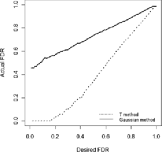
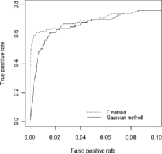
(a)	(b)

Figure 2: Comparison of the results analyzed by the T method and the Gaussian method, based on data generated from $t$-distributions with $J=2$. (a) The actual FDR versus the desired FDR; (b) the ROC curves.

The second data set is generated by the same model parameters as the first data set except $\omega_{x_{ij}}=\omega_{y_{ij}}=1$, $\sigma_{x_{i}}^{2}=0.1$, and $\sigma_{y_{i}}^{2}=0.5$; thus, the error terms are normal with the same variance. This data set is again analyzed by the above-mentioned T method and the Gaussian method and a comparison of the two is summarized in Figure 3. We can see that the Gaussian method performs only slightly better.

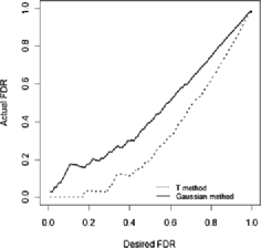
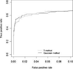
(a)	(b)

Figure 3: Comparison of the results analyzed by the T method and the Gaussian method, based on data generated by normal distribution with $J=2$. (a) The actual FDR versus the desired FDR; (b) the ROC curves.

The third data set is generated in the same way as the first except that the number of replicates $J=10$. Figure 4 compares the results obtained from the data with $J=2$ and $J=10$, both of which are analyzed by the T method of this paper. Figure 4 shows that the results using $J=10$ is much better than $J=2$.

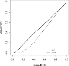
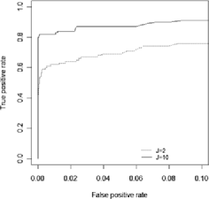
(a)	(b)

Figure 4: Comparison of the results with $J=2$ and $J=10$, based on data generated from $t$-distributions and analyzed by the T method. (a) The actual FDR versus the desired FDR; (b) the ROC curves.

In fact, we also compared these two methods using data generated with error terms being neither Gaussian nor $t$-distributed and observed results similar to those in Figures 2 and 4. To keep the paper concise, we omit reporting these comparisons.

4 Data preprocessing

Data preprocessing for RNAi HTS usually consists of three parts: edge effect adjustment, normalization to reduce plate effects, and outlier removal. Several data preprocessing methods have been proposed to deal with these issues; see, for example, Boutros, Bras and Huber (2006), Malo et al. (2006) and Zhang et al. (2006). These methods are adapted to suit the present experiment.

The following three observations motivate our data preprocessing procedure. The first observation is that technically replicated measurements should be close to each other; this provides an opportunity to evaluate the general quality of the experiment as well as to eliminate shRNAs showing large discrepancy between the replicated measurements. The second observation is that the assignment of a shRNA to a well and the effect of this shRNA on the measurements are independent; our edge-effect adjustment makes use of this observation. The third observation is that measurements of control wells of the same type are expected to be close to each other; the measurements for NTNP wells are expected to be larger than those for SN wells and those for NTWP wells are expected to have the smallest measurements; violation of these indicates poor quality of the experiments. In the HCV study, no such violation is observed in any single plate either for luciferase activity or cell viability; our normalization procedure makes use of this observation.

Our data preprocessing are performed by first conducting edge effect adjustment and selecting the control wells so as to perform normalization, and then deleting the outliers. The final data in the analysis consists of $6\mbox{,}130$ shRNA and $419$ negative control wells, each of which has four replicates.

Control wells serve two purposes in our data preprocessing. Since the measurements for NTNP wells are larger than those for SN wells and NTWP wells have the smallest measurements in any plate, it seems a good idea to use these control wells to perform normalization if we can first delete outliers in the control wells. This outlier deletion is carried out for luciferase activity and cell viability separately. Here we present the deletion criterion for the luciferase activity in a shRNA or control well; that for cell viability is similar and omitted. Using the fact that there are four platewise replicates with two of them measuring luciferase activity, we consider the ratio of the difference of its two replicated measurements to its mean for a given well position, and delete both of its luciferase activities for a given well position if the ratio is large. For the HCV study data, two NTNP control wells were deleted based on the cell viability measurement before normalization.

Edge effect exists in both the measurements of luciferase activity and cell viability; the same adjustment procedure is carried out separately for each of these two measurements and described as follows. We partition all the wells in this experiment into three groups: G1 consists of all the wells on the boundary of a plate; G2 consists of all the wells not in G1 but immediately adjacent to wells in G1; G3 the remaining wells. A fixed constant is added to the measurement from each well in G2 so that the average of all the measurements from wells in G2 is equal to that from wells in G3; a similar procedure is applied to the measurements from each well in G1, except those from NTWP control wells. The rationale for not performing edge effect adjustment to the NTWP control wells is that the total numbers of cells in these wells are very small already and we expect little edge effects there. We note that all the control wells are in G1.

After the outliers in the controls have been removed and the edge effect has been taken into account, we perform normalization to reduce the plate effect. The same normalization procedure is done separately for luciferase activity and cell viability; we describe the procedure for luciferase activity and omit that for cell viability, because of the similarity. Our normalization will, in particular, make mean measurements of the controls of the same type in each plate taking the same value for different plates. The procedure is as follows. We denote the mean measurements of NTNP wells, SN wells, and NTWP wells in plate $h$ by $a_{h}$, $b_{h}$, and $c_{h}$, respectively. Let $a$, $b$, and $c$ denote, respectively, the mean measurements of all of the NTNP wells, SN wells, and NTWP wells from all the plates in this experiment. The normalization procedure for wells in plate $h$ is accomplished by using the unique continuous piecewise linear function that maps $a_{h}$, $b_{h}$, and $c_{h}$ to $a$, $b$, and $c$, respectively. Namely, its value at $x$ is

$$\cases{x-c_{h}+c,&\quad if $x\leq c_{h}$;\cr(a-c)(x-c_{h})/(a_{h}-c_{h})+c,&\quad if $c_{h}<x\leq a_{h}$;\cr(b-a)(x-a_{h})/(b_{h}-a_{h})+a,&\quad if $a_{h}<x\leq b_{h}$;\cr x-b_{h}+b,&\quad if $b_{h}<x$.}$$

The luciferase activity of a well in plate $h$ is to be replaced by the value of the piecewise linear function at that luciferase activity. In the plates without NTWP wells, the normalization is carried out using the piecewise linear function defined by $a$ and $b$.

After normalization, we exclude a shRNA from the analysis if either the ratio of the difference of its two replicated luciferase activity to its mean or the ratio corresponding to its two replicated cell viability measurements is large. For each of the two measurements, we excluded two percent of the shRNAs that have the most extreme ratios in the HCV study.

5 The HCV study

We now apply our methods to analyze the HCV study data. In particular, we will provide lists of candidate shRNAs causing the reduction of HCV replication without changing cell viability. We will first explain in some detail the way we apply the methods in analyzing the data and the way we use part of the control wells to evaluate the performance of the methods. We will also examine our methods in light of a limited Q-PCR experiment, compare with the results using the standard $Z$-score approach, show that our Bayesian analysis is insensitive to the choice of prior, and indicate that there does exist concordance between our findings and those in Supekova et al. (2008) and Tai et al. (2009).

5.1 Data analysis

After the data preprocessing procedures, we analyzed the data using the Bayesian method of this paper. Following the data analysis strategies described in Section 2, we choose $\phi_{1}=\phi_{2}=0.03$ and $\phi_{3}=\phi_{4}=0.2$. In fact, $\{(x_{i1}-x_{i2})^{2}/2|i=1,\ldots,6\mbox{,}549\}$ has mean $0.0016$ and variance $8\times 10^{-6}$ and $\{(y_{i1}-y_{i2})^{2}/2|i=1,\ldots,6\mbox{,}549\}$ has mean $0.0107$ and variance $0.0004$. Except for the sensitivity analysis in Section 5.5, we always use $\phi_{5}=9$, $\phi_{6}=1$, $\phi_{7}=3$, and $\phi_{8}=1.9\times 10^{5}$ in this section. We note that $\operatorname{IG}(\cdot|3,1.9\times 10^{5})$ has mean $95\mbox{,}000$ and variance $9.025\times 10^{9}$.

We use about half of the SN and NTNP wells and all of the NTWP wells for normalization purposes and use the remaining control wells to evaluate our analysis method and to help decide the knockdown effects of specific shRNAs. In each plate, there is about one NTWP well, two SN wells, and three NTNP wells. We use all the NTWP wells for normalization. We also note that there are in total $71$ plates and $426$ control wells in one replicate and there are four platewise replicates, as described at the end of Section 1.1. After the initial outlier deletion of $2$ NTNP controls, we use $277$ controls for normalization. The outlier deletion step after normalization excluded another $6$ controls, three of which were among those used for normalization earlier. These outliers are excluded from the analysis. It turns out that our analysis includes $419$ controls, $274$ of which were used for normalization and the remaining $145$ controls are used to evaluate our methods as well as to decide the knockdown effect of specific shRNAs.

The posterior distributions are obtained by the hybrid MCMC algorithm in the supplementary material [Chen et al. (2011)]. We calculated the Gelman–Rubin statistic $\hat{R}$ for all the important estimands based on five chains with random initial values in several studies and found all the $\hat{R}$’s were less then $1.1$ using the iterations between $10\mbox{,}000$ and $20\mbox{,}000$. Based on this experience and the fact that all the studies in this section involve similar computations, we run one chain with $40\mbox{,}000$ iterations and use the latter $20\mbox{,}000$ iterations to calculate the posterior distributions of all the parameters in each study.

Figure 5: The volcano plot of posterior activity change coefficient and posterior probability of activity change for the HCV study.

Figure 5 gives some idea of the distribution of the activity change in this experiment. Each dot in Figure 5 gives the results of one shRNA; its vertical coordinate gives its posterior probability of incurring activity change $1-p_{i}$ and its horizontal coordinate gives its magnitude of activity change $E(\beta_{i}|\gamma_{i}=1,x,y)$, given there is activity change. $E(\beta_{i}|\gamma_{i}=1,x,y)$ is also called the posterior activity change coefficient. Figure 5 indicates a very clear relation between these two quantities and it will be clear that both are useful in examining the activity change.

Figure 6: The Scatterplot of predictive versus realized $\chi^{2}$ discrepancies for the HCV study.

Figure 6 gives the graphical display of the posterior predictive check that using the $\chi^{2}$ omnibus discrepancy test quantity,

$$\sum_{i=1}^{6\mbox{,}549}\sum_{j=1}^{2}\frac{(y_{ij}-\alpha_{0}-\gamma_{i}\beta_{i}-\alpha_{1}x_{ij})^{2}}{\alpha_{1}^{2}\sigma_{x_{i}}^{2}d_{x}/(d_{x}-2)+\sigma_{y_{i}}^{2}d_{y}/(d_{y}-2)}.$$

The concept of posterior predictive check appeared in Gelman, Meng and Stern (1996); see also Gelman et al. (2003). Figure 6 seems to indicate that the model fits the data quite well. In fact, in the choice of priors, we find large $\phi_{8}$ not only makes $V$ less informative but also make model fit possible. By the way, the posterior means of $\alpha_{0}$, $\alpha_{1}$, $V$, $d_{x}$, and $d_{y}$ are, respectively, $12.557$, $2.538$, $58.207$, $30$, and $10$.

We may regard the minimal interval containing the posterior means of the cell viability $E(\mu_{i}|x,y)$ of the $274$ controls as the range of normal cell viability, which is $(-0.635,-0.007)$, although this definition of normal cell viability might be a little too stringent. Nevertheless, we find all of the remaining $145$ controls are in this normal range. This finding seems to suggest that our methods give good estimates of the cell viabilities. Among all the $6\mbox{,}130+419=6\mbox{,}549$ wells, $5\mbox{,}862$ have their cell viabilities in the normal range, $602$ of them less than $-0.635$ and $85$ of them larger then $-0.007$.

Figure 7 reports two histograms of the probability of activity change $1-p_{i}$. The dark one, called Histogram 7(a), is the histogram for the $145$ controls; the light one, called Histogram 7(b), is that for all the $6\mbox{,}549$ wells. Since Histogram 7(a) concentrates heavily on the left, we think our methods assigned appropriate posterior probability to these $145$ control wells.

In fact, Histogram 7(a) provides opportunities for the study of false discovery rate. For this, we present the data of Histogram 7(a) in Figure 8 using finer resolution so as to exhibit more details. Figure 8 seems to suggest that the set of shRNAs having $1-p_{i}$ larger than $0.2532$, $0.1055$, or $0.05$ has false discovery rate, respectively, $0$, $1/145$, or $2/145$, among others.

Figure 7: Histogram of posterior probability of activity change $1-p_{i}$. The dark histogram, referred to as Histogram 7(a), is for the $145$ control wells reserved for evaluation purposes. The light histogram, referred to as Histogram 7(b), is for all the $6\mbox{,}549$ wells.

Figure 8: Histogram of the posterior probability of activity change $1-p_{i}$ for the $145$ control wells.

There is still another quantity that is useful in assessing the performance of our methods, namely, the posterior activity change coefficient $E(\beta_{i}|\gamma_{i}=1,x,y)$. Figure 9 provides two histograms of posterior activity change coefficient; the dark one, sitting above the interval $(-0.806,0.392)$, is that for the $145$ shRNAs in the control wells and the light one, sitting above the interval $(-4.081,1.967)$, is that for the total set of $6\mbox{,}549$ shRNAs. The fact that the former sits in the middle of the latter, as expected, seems to give another piece of indication that the experiment and data analysis are reliable.

5.2 Main results

We are now in a position to provide shRNA lists, based on which the laboratory scientists can conduct experiments to identify those that affect HCV replication without affecting cell viability. Knowing that among the $785$ shRNAs having their $E(\beta_{i}|\gamma_{i}=1,x,y)$ less than $-0.806$, $601$ of them have their cell viability in the normal range $(-0.635,-0.007)$, we will start the selection with this set of $601$ shRNAs. For this, we will make use of the direct posterior probability approach discussed in Newton et al. (2004).

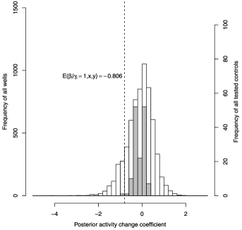
Figure 9: Histogram of posterior activity change coefficients. The dark histogram is for the $145$ control wells. The light histogram is for all the $6\mbox{,}549$ wells.

Assuming that placing a shRNA having posterior probability of not incurring activity change $p_{i}$ in the list for further studies creates a loss of the amount $p_{i}$, we rank the shRNAs according to their $p_{i}$ and form the list as follows. Given a set $\varsigma$ of shRNAs for which the losses are less than a positive number $\kappa$, we define

$$C(\kappa)=\sum_{i}p_{i}1_{[p_{i}<\kappa]},$$

which is the sum of the losses for all the shRNAs in $\varsigma$. We note that $C(\kappa)/|\varsigma|$ is called the posterior false detections rate (PFDR), where $|\varsigma|$ is the size of the set $\varsigma$; we also note that with the shRNAs ordered by $p_{i}$, there is a natural correspondence between $\kappa$ and set size $|\varsigma|$ and that $C(\kappa)/|\varsigma|$ increases with $\kappa$. To obtain a list of shRNAs having PFDR $C(\kappa)/|\varsigma|$ less than $\alpha$, we can find the largest possible $\kappa$ or $|\varsigma|$ such that $C(\kappa)/|\varsigma|$ is less than $\alpha$. In practice, we can either fix the list size and then compute its PFDR or fix the PFDR and compute the list size. For the set of $601$ shRNAs having normal cell viability and posterior activity change coefficient less than $-0.806$, Table 1 is a summary of various lists of shRNAs. Its left column reports PFDR by first fixing the set size and its right column reports list size by first fixing the PFDR. For example, the second row in the left column says that the list of top $100$ candidate shRNAs, targeting $77$ genes, has PFDR $0.047$; the second row of the right column says given PFDR being $0.05$, the list has $104$ shRNAs, targeting $81$ genes, and one of the genes has three of the $104$ shRNAs targeting it, $21$ of the genes have two such shRNAs targeting each of them and the remaining $59$ genes have only one such shRNA targeting each of them.

Table 1: Posterior false detection rates for lists of shRNAs whose $E(\mu_{i}|x,y)\in(-0.635,-0.007)$ and $E(\beta_{i}|\gamma_{i}=1,x,y)<-0.806$ in the HCV study

Fix list size		Fix PFDR
1-2,3-9
	Number of genes (shRNAs)		Number of genes (shRNAs)	Number of shRNAs
PFDR		PFDR		5	4	3	2	1
0.024	040 (50)0	0.01	20 (21)				1	19
0.047	077 (100)	0.05	081 (104)			1	21	59
0.106	151 (200)	0.10	144 (190)		2	6	27	109
0.174	210 (300)	0.20	234 (337)	1	3	15	57	158
0.242	271 (400)	0.30	309 (488)	3	7	31	79	189

We note that when we are interested in individual shRNAs, those in the first row are better candidates than those in the other rows; when we are interested in genes that affect HCV replication, then we need to consider the number and the knockdown effects of all the shRNAs in each gene. We will illustrate the latter in Section 5.6.

Tai et al. (2009) pointed out the issue of the choice of threshold in the $Z$-score approach to hit selection; higher threshold causes little overlap with other studies and lower threshold results in too many siRNAs for secondary validation. Our approach benefits from not only the statistical model but also the negative controls. The above analysis points out an issue regarding the number of negative controls to be used for the false discovery rate estimate. We believe that if we had more negative controls, we could have provided more information, including false discovery rate, for the selection of shRNAs or genes.

For the purpose of comparison in Sections 5.4 and 5.6, we say a shRNA in the HCV study causes activity change if either its $p_{i}<1-0.2532=0.7468$ or its $E(\beta_{i}|\gamma_{i}=1,x,y)\notin[-0.806,0.392]$; a shRNA has normal cell viability if its $E(\mu_{i}|x,y)\in(-0.635,-0.007)$.

5.3 Q-PCR validation

Q-PCR is one of the popular methods to study activity change in a secondary analysis of a gene list from a primary RNAi HTS. In this study, both HCV RNA and house-keeping gene beta-actin are reverse transcribed and then quantified using Q-PCR in a well with a given shRNA or without any shRNA transduction. The ratio of the quantity of HCV RNA in a well with the shRNA transduction to that in a well without any shRNA transduction and the corresponding ratio for beta-actin are first calculated; the former ratio divided by the latter ratio gives the activity change measured by Q-PCR for shRNA $i$, which is denoted by $k_{i}$.

When $k_{i}$ is around $1$, we may say there is no activity change; when it is large (small), we may say it increases (decreases) the activity. Although Q-PCR is considered to provide reliable measurements, we do not know of a good threshold on $k_{i}$ for declaring activity change. Thus, we choose to present the correlation between the activity $k_{i}$ reported by the Q-PCR assay and posterior activity change coefficient reported by our methods as a way to make the comparison.

We examined by the Q-PCR method the pathway activity of $86$ shRNAs in the HCV study; we note that $68$ of them have their ratio for beta-actin belonging to the interval $(0.7,1.43)$; these $68$ shRNAs may thus be considered to have less appreciable effect on cell viability. The empirical correlations of these two assays are $0.68$ for all these $86$ shRNAs and $0.77$ for the $68$ shRNAs not affecting cell viability. We note that these $86$ shRNAs had been chosen for Q-PCR assay before the methods of this paper were proposed. We note that we do not expect perfect correlation, because, for HCV replication, our RNAi HTS monitors the luciferase protein and Q-PCR measures HCV RNA and, for cell viability, ours monitors the level of dehydrogenase and Q-PCR montiors the level of mRNA of beta-actin.

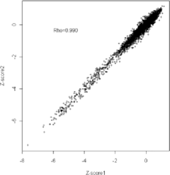
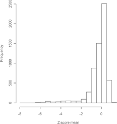
(a)	(b)

Figure 10: Scatter plot for $Z$-scores and histogram of $Z$-score mean. (a) The scatter plot for $(Z_{i1},Z_{i2})$; (b) the histogram of $Z_{i}=(Z_{i1}+Z_{i2})/2$.

5.4 Comparison with the $Z$-score approach

Platewise $Z$-score is often used in the primary analysis of RNAi HTS data; see, for example, Tai et al. (2009). In particular, Tai et al. (2009) says that “A $Z$-score is the number of standard deviations of the experimental luciferase activity above the median plate value.” Because the plate effect in the data from the HCV study has been reduced by normalization, it seems appropriate for us to consider an experiment-wise $Z$-score and compare this $Z$-score approach with the method of this paper. We define the $Z$-score as

$$Z_{ij}=\frac{y_{ij}-M_{j}}{S_{j}}.$$

Here $M_{j}$ and $S_{j}$ are, respectively, the median and standard deviation of $\{y_{ij}|i=1,\ldots,I\}$ for $j=1,2$, after data preprocessing procedures.

Hit selection based on $Z$-score chooses shRNAs having extreme $Z$-scores. It is desirable that these $Z$-scores follow a normal distribution; in this case, we can conveniently assign a $p$-value to $Z_{i}=(Z_{i1}+Z_{i2})/2$ and use $p$-value to describe the extremeness of the selected shRNA. Figures 10(a) and (b) give, respectively, the plot of $(Z_{i1},Z_{i2})$ and the histogram of $\{Z_{i}|i=1,\ldots,I\}$ for the HCV study. While Figure 10(a) shows that $Z_{i1}$ and $Z_{i2}$ have correlation $0.990$ and are in good agreement, indicating both the assay and the data preprocessing procedure are excellent, Figure 10(b) suggests they are not normally distributed.

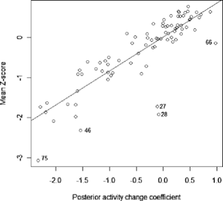
Figure 11: Plot of the $Z$-score vs posterior activity change coefficient for $86$ shRNAs. The shRNAs that show largest discrepancy between the $Z$-score and posterior activity change coefficient target, respectively, RPS6, KIAA1446, INPP4A, SFRS1, and TYK2. The numerals in the figure correspond to those in Table 2.

For the above set of $86$ shRNAs assayed by Q-PCR and whose subset of $68$ shRNAs are not affecting cell viability, we find the empirical correlations of their $Z$-scores $Z_{i}$ and the activity change measured by Q-PCR $k_{i}$ are $0.62$ and $0.72$, respectively. Compared with the correlations reported in Section 5.3, it seems that the activity change computed by our method is in better agreement with those reported by the Q-PCR method.

Figure 11 is the plot of the $Z_{i}$ versus $E(\beta_{i}|\gamma_{i}=1,x,y)$ for the $86$ shRNAs. The five shRNAs that show largest discrepancy between the $Z$-score $Z_{i}$ and posterior activity change coefficient target five genes: RPS6, KIAA1446, INPP4A, SFRS1, and TYK2; this discrepancy is decided by the size of the residues when a linear regression is fitted. Table 2 reports the posterior probability of activity change, posterior activity change coefficient, posterior mean of cell viability $E(\mu_{i}|x,y)$, $Z$-score $Z_{i}$, and Q-PCR activity change $k_{i}$ for these five shRNAs showing largest discrepancy. All these methods claim unequivocally and unanimously that the shRNA targeting RPS6 decreases the pathway activity significantly. In fact, we have verified that RPS6 is a crucial factor for HCV and we are preparing a manuscript for this finding. Both Q-PCR and our method claim that the one targeting KIAA1446 increases the activity of the pathway and that targeting INPP4A has little effect on the pathway, while the $Z$-score approach suggests differently; for SFRS1, Q-PCR seems to claim a mild increase of the pathway activity, our method suggests little effect on the pathway activity and $Z$-score suggests a decrease in pathway activity; for TYK2, Q-PCR suggests little effect and both our method and $Z$-score suggest a decrease in pathway activity. Table 2 seems to suggest again that our method is in better agreement with the Q-PCR method in reporting the activity change effects of shRNAs. We note that the percentage in the cell viability in Table 2 shows the corresponding percentile among all the $6\mbox{,}549$ wells.

Table 2: The $Z$-score, posterior activity change coefficient, and Q-PCR activity change effect $k_{i}$ for five shRNAs

	Gene	$\bolds{1-p_{i}}$	$\bolds{E(\beta_{i}|\gamma_{i}=1,x,y)}$	$\bolds{E(\mu_{i}|x,y)}$	$\bolds{Z_{i}}$	$\bolds{k_{i}}$
75	RPS6	0.993	$-2.323$	$-$0.657 (8.80%)	$-3.067$	0.08
66	KIAA1446	0.491	$0.973$	$-$0.657 (8.81%)	$-0.134$	2.59
28	INPP4A	0.005	$-0.088$	$-$1.065 (6.00%)	$-1.925$	1.25
27	SFRS1	0.005	$-0.111$	$-$0.975 (6.41%)	$-1.719$	1.83
46	TYK2	0.907	$-1.542$	$-$0.650 (8.95%)	$-2.317$	1.33

5.5 Sensitivity analysis

This subsection examines certain distributional assumptions on the prior used in Section 5.1 for analyzing the HCV study data. The prior on $p$ used was $\operatorname{\mathcal{B}eta}(9,1)$; we now also consider $\operatorname{\mathcal{B}eta}(1,1)$. The prior on $\mu_{i}$ was $\mathcal{U}(-3,1)$; we now also consider the empirical one $(0.248+2.77)\cdot\operatorname{\mathcal{B}eta}(6,2)-2.77$. Thus, there are four combinations in these comparisons, with all the other analysis strategies unchanged. We report here three posterior inferences for the comparison of these four studies. In fact, we made extensive comparisons and found only similar results and the three reported here are the most representative ones. Table 3 treats the

Table 3: Posterior probability of incurring activity change $1-p_{i}$ for the $145$ control wells

Prior on $\bolds{p}$	$\bolds{\operatorname{\mathcal{B}eta}(9,1)}$		$\bolds{\operatorname{\mathcal{B}eta}(1,1)}$
2-3,4-5
Prior on $\bolds{\mu_{i}}$	Empirical prior	Uniform prior	Empirical prior	Uniform prior
Median	0.0045	0.0068	0.0043	0.0038
75% quantile	0.0095	0.0155	0.0078	0.0065
Maximum	0.1275	0.2532	0.1098	0.0955

posterior probability of activity change based on the $145$ controls. That all these probabilities in Table 3 are close to zero shows that all of them perform very well, just as the one in Section 5.1. Table 4 reports

Table 4: Correlations between the posterior probability of activity change obtained from one prior combination and that from another

Prior on $\bolds{p}$		$\bolds{\operatorname{\mathcal{B}eta}(9,1)}$		$\bolds{\operatorname{\mathcal{B}eta}(1,1)}$
3-4,5-5
	Prior on $\bolds{\mu_{i}}$	Empirical prior	Uniform prior	Empirical prior
$\operatorname{\mathcal{B}eta}(9,1)$	Empirical prior
	Uniform prior	0.972
$\operatorname{\mathcal{B}eta}(1,1)$	Empirical prior	0.997	0.960
	Uniform prior	0.992	0.946	0.995

Table 5: Correlations between the posterior activity change coefficient obtained from one prior combination and that from another

Prior on $\bolds{p}$		$\bolds{\operatorname{\mathcal{B}eta}(9,1)}$		$\bolds{\operatorname{\mathcal{B}eta}(1,1)}$
3-4,5-5
	Prior on $\bolds{\mu_{i}}$	Empirical prior	Uniform prior	Empirical prior
$\operatorname{\mathcal{B}eta}(9,1)$	Empirical prior
	Uniform prior	0.990
$\operatorname{\mathcal{B}eta}(1,1)$	Empirical prior	0.992	0.988
	Uniform prior	0.990	0.988	0.989

the correlation between the probability of activity change obtained from one combination and that obtained from another. Table 5, like Table 4, reports the correlation regarding the posterior activity change coefficient obtained from different analyses. Since all of the correlations in Table 4 and Table 5 are larger than $0.94$, it seems that the posterior inferences are not sensitive to these aspects of the prior assumptions.

5.6 Some comparison with the literature

Cherry (2009) reviewed five papers that use siRNA screens to identify cellular factors that impact replication of HCV or subgenomic replicons and found little overlap between them. As part of our effort to evaluate the performance of our method, we select all the siRNAs in our list that show activity change in Supekova et al. (2008) and Tai et al. (2009) and see whether our findings are in line with theirs. A comprehensive discussion of the scientific findings of our study will be reported elsewhere.

Supekova et al. (2008) reported that siRNAs specific for three human kinases, CSK, JAK1, and VRK1, were identified to reduce the replication of HCV; they also reported that by examining the siRNA knockdown effect of the eight kinase genes in the Src family (BLK, HCK, FGR, LCK, LYN, FYN, c-SRC, and YES) on the HCV replicon, they found that their siRNAs targeting seven of them did not show any effect and that targeting FYN elevated replicon levels by about 3-fold upon transduction.

In our HCV study, there are shRNAs targeting nine of these $11$ genes, except c-SRC and YES. We now compare our results on these nine genes with those from Supekova et al. (2008).

Among the five shRNAs targeting FYN, four of them indicated considerable elevation in HCV replication and the other one did not show activity change; none showed change in cell viability. Our screening showed also that none of the shRNA targeting FGR or HCK indicated any appreciable activity change. These results are in perfect or excellent agreement with those in Supekova et al. (2008).

Among the four targeting BLK, three of them showed no activity change and one indicated considerable increase; among the five targeting LCK, four of them showed no activity change and one indicated considerable decrease. These are in partial agreement with Supekova et al. (2008).

Among the $10$ shRNAs targeting CSK, one showed considerable decrease both in HCV replication and in cell viability; another showed considerable decrease in HCV replication without change in cell viability; still another showed considerable increase in HCV replication without change in cell viability; the remaining seven showed no change. All the four targeting JAK1 indicated no activity change and no cell viability change. None of the two targeting VRK1 indicated any appreciable activity change, although one of them indicated considerable reduction in cell viability. Among the five shRNAs targeting LYN, three of them indicated strong elevation in HCV replication without appreciable change in cell viability. These suggest a certain amount of disagreement between our findings and those in Supekova et al. (2008).

In view of the general lack of concordance between results of similar HCV screens in the literature, the amount of agreement between Supekova et al. (2008) and our study seems encouraging.

We note that Tai et al. (2009) reported that there is little overlap between the results of their screen and those of Supekova et al. (2008); in fact, none of the three genes CSK, JAK1, and VKR1 were selected in the primary screening of Tai et al. (2009), which seems to be in agreement with ours.

We now compare our results with Tai et al. (2009), in which $96$ genes are chosen from the primary screening for reduced HCV replication. In the shRNA list of our study, there are shRNAs targeting four of these $96$ genes; they are TBK1, NUAK2, COASY, and MAP3K14.

Two of the four shRNAs in our list targeting MAP3K14 showed strong reduction in HCV replication, another indicated marginal reduction in HCV replication and the fourth one indicated no activity change; none showed change in cell viability. The shRNAs targeting the remaining three genes showed little effect on the reduction of HCV replication. We note that Tai et al. (2009) used $21\mbox{,}094$ siRNA pools targeting the entire human RefSeq transcript database; each of these pools consists of four individual siRNA duplexes and each of these four siRNAs targets a different sequence within the target transcript.

6 Discussion

We have presented a Bayesian method to analyze data from two channel cell-based RNAi HTS experiments with replicates, in which the phenotype of a pathway-specific reporter gene and that of a constitutive reporter are measured. These experiments are typical in screens for signaling pathway components and the purpose is often to identify genes that affect the activity of the specific pathway without affecting that of the constitutive reporter.

We have conducted simulation studies and real data analysis to illustrate the methods. Our simulation studies indicate that error terms with shRNA specific $t$-distribution do make the method flexible and robust and that replication provides better power in identifying shRNAs of interests and, at the same time, gives better estimates of the false discovery rates.

In our analysis of the real data set, we illustrate the usage of negative controls, included originally for normalization purposes only, to assess the performance of our methods, to estimate false discovery rate, and to prioritize the shRNAs for secondary validation, in addition to hit selection; we find our methods perform excellently and these negative controls are very useful. We have also conducted a Q-PCR based assay to assess the activity change of $86$ shRNAs; we find the results based on Q-PCR are in better agreement with those based on our method than with those based on the standard $Z$-score approach. We have also shown that our method is insensitive to the choice of prior. Finally, it is encouraging to find that there does exist some overlap between the results of the HCV study and those of Supekova et al. (2008) and Tai et al. (2009).

Realizing the usefulness of negative controls, we are interested in knowing the optimal number of negative controls to be included in an experiment. It seems also desirable to include positive controls as well in the experiment. With both positive and negative controls, we may extend our Bayesian method so as to improve our report on the false positive and negative rates in a RNAi HTS. We note that characteristics of these controls, especially positive controls, and the number of these controls deserve serious attention in designing an experiment and in extending our statistical method.

References

- Birmingham et al. (2009) {barticle}[pbm] \bauthor\bsnmBirmingham, \bfnmAmanda\binitsA., \bauthor\bsnmSelfors, \bfnmLaura M.\binitsL. M., \bauthor\bsnmForster, \bfnmThorsten\binitsT., \bauthor\bsnmWrobel, \bfnmDavid\binitsD., \bauthor\bsnmKennedy, \bfnmCaleb J.\binitsC. J., \bauthor\bsnmShanks, \bfnmEmma\binitsE., \bauthor\bsnmSantoyo-Lopez, \bfnmJavier\binitsJ., \bauthor\bsnmDunican, \bfnmDara J.\binitsD. J., \bauthor\bsnmLong, \bfnmAideen\binitsA., \bauthor\bsnmKelleher, \bfnmDermot\binitsD., \bauthor\bsnmSmith, \bfnmQueta\binitsQ., \bauthor\bsnmBeijersbergen, \bfnmRoderick L.\binitsR. L., \bauthor\bsnmGhazal, \bfnmPeter\binitsP. and \bauthor\bsnmShamu, \bfnmCaroline E.\binitsC. E. (\byear2009). \btitleStatistical methods for analysis of high-throughput RNA interference screens. \bjournalNat. Methods \bvolume6 \bpages569–575. \biddoi=10.1038/nmeth.1351, issn=1548-7105, mid=NIHMS159092, pii=nmeth.1351, pmcid=2789971, pmid=19644458 \bptokimsref \endbibitem
- Börner et al. (2010) {barticle}[pbm] \bauthor\bsnmBörner, \bfnmKathleen\binitsK., \bauthor\bsnmHermle, \bfnmJohannes\binitsJ., \bauthor\bsnmSommer, \bfnmChristoph\binitsC., \bauthor\bsnmBrown, \bfnmNigel P.\binitsN. P., \bauthor\bsnmKnapp, \bfnmBettina\binitsB., \bauthor\bsnmGlass, \bfnmBärbel\binitsB., \bauthor\bsnmKunkel, \bfnmJulian\binitsJ., \bauthor\bsnmTorralba, \bfnmGloria\binitsG., \bauthor\bsnmReymann, \bfnmJürgen\binitsJ., \bauthor\bsnmBeil, \bfnmNina\binitsN., \bauthor\bsnmBeneke, \bfnmJürgen\binitsJ., \bauthor\bsnmPepperkok, \bfnmRainer\binitsR., \bauthor\bsnmSchneider, \bfnmReinhard\binitsR., \bauthor\bsnmLudwig, \bfnmThomas\binitsT., \bauthor\bsnmHausmann, \bfnmMichael\binitsM., \bauthor\bsnmHamprecht, \bfnmFred\binitsF., \bauthor\bsnmErfle, \bfnmHolger\binitsH., \bauthor\bsnmKaderali, \bfnmLars\binitsL., \bauthor\bsnmKräusslich, \bfnmHans-Georg\binitsH.-G. and \bauthor\bsnmLehmann, \bfnmMaik J.\binitsM. J. (\byear2010). \btitleFrom experimental setup to bioinformatics: An RNAi screening platform to identify host factors involved in HIV-1 replication. \bjournalBiotechnol. J. \bvolume5 \bpages39–49. \biddoi=10.1002/biot.200900226, issn=1860-7314, pmid=20013946 \bptokimsref \endbibitem
- Boutros and Ahringer (2008) {barticle}[pbm] \bauthor\bsnmBoutros, \bfnmMichael\binitsM. and \bauthor\bsnmAhringer, \bfnmJulie\binitsJ. (\byear2008). \btitleThe art and design of genetic screens: RNA interference. \bjournalNat. Rev. Genet. \bvolume9 \bpages554–566. \biddoi=10.1038/nrg2364, issn=1471-0064, pii=nrg2364, pmid=18521077 \bptokimsref \endbibitem
- Boutros, Bras and Huber (2006) {barticle}[pbm] \bauthor\bsnmBoutros, \bfnmMichael\binitsM., \bauthor\bsnmBras, \bfnmLígia P.\binitsL. P. and \bauthor\bsnmHuber, \bfnmWolfgang\binitsW. (\byear2006). \btitleAnalysis of cell-based RNAi screens. \bjournalGenome Biol. \bvolume7 \bpagesR66. \biddoi=10.1186/gb-2006-7-7-R66, issn=1465-6914, pii=gb-2006-7-7-R66, pmcid=1779553, pmid=16869968 \bptokimsref \endbibitem
- Box and Cox (1964) {barticle}[mr] \bauthor\bsnmBox, \bfnmG. E. P.\binitsG. E. P. and \bauthor\bsnmCox, \bfnmD. R.\binitsD. R. (\byear1964). \btitleAn analysis of transformations. \bjournalJ. R. Stat. Soc. Ser. B Stat. Methodol. \bvolume26 \bpages211–252. \bidissn=0035-9246, mr=0192611 \bptnotecheck related\bptokimsref \endbibitem
- Chapman and Carrington (2007) {barticle}[pbm] \bauthor\bsnmChapman, \bfnmElisabeth J.\binitsE. J. and \bauthor\bsnmCarrington, \bfnmJames C.\binitsJ. C. (\byear2007). \btitleSpecialization and evolution of endogenous small RNA pathways. \bjournalNat. Rev. Genet. \bvolume8 \bpages884–896. \biddoi=10.1038/nrg2179, issn=1471-0064, pii=nrg2179, pmid=17943195 \bptokimsref \endbibitem
- Chen et al. (2011) {bmisc}[auto:STB—2011/08/30—13:45:12] \bauthor\bsnmChen, \bfnmC. H.\binitsC. H., \bauthor\bsnmSu, \bfnmW. C.\binitsW. C., \bauthor\bsnmChen, \bfnmC. Y.\binitsC. Y., \bauthor\bsnmHuang, \bfnmJ. Y.\binitsJ. Y., \bauthor\bsnmTsai, \bfnmF. Y.\binitsF. Y., \bauthor\bsnmWang, \bfnmW. C.\binitsW. C., \bauthor\bsnmHsiung, \bfnmC. A.\binitsC. A., \bauthor\bsnmJeng, \bfnmK. S.\binitsK. S. and \bauthor\bsnmChang, \bfnmI. S.\binitsI. S. (\byear2011). \bhowpublishedSupplement to “A Bayesian measurement error model for two-channel cell-based RNAi data with replicates.” DOI:10.1214/11-AOAS496SUPP. \bptokimsref \endbibitem
- Cherry (2009) {barticle}[pbm] \bauthor\bsnmCherry, \bfnmSara\binitsS. (\byear2009). \btitleWhat have RNAi screens taught us about viral-host interactions? \bjournalCurr. Opin. Microbiol. \bvolume12 \bpages446–452. \biddoi=10.1016/j.mib.2009.06.002, issn=1879-0364, mid=NIHMS129820, pii=S1369-5274(09)00075-7, pmcid=2766546, pmid=19576842 \bptokimsref \endbibitem
- Cleveland (1979) {barticle}[mr] \bauthor\bsnmCleveland, \bfnmWilliam S.\binitsW. S. (\byear1979). \btitleRobust locally weighted regression and smoothing scatterplots. \bjournalJ. Amer. Statist. Assoc. \bvolume74 \bpages829–836. \bidissn=0003-1291, mr=0556476 \bptokimsref \endbibitem
- Echeverri et al. (2006) {barticle}[pbm] \bauthor\bsnmEcheverri, \bfnmChristophe J.\binitsC. J., \bauthor\bsnmBeachy, \bfnmPhilip A.\binitsP. A., \bauthor\bsnmBaum, \bfnmBuzz\binitsB., \bauthor\bsnmBoutros, \bfnmMichael\binitsM., \bauthor\bsnmBuchholz, \bfnmFrank\binitsF., \bauthor\bsnmChanda, \bfnmSumit K.\binitsS. K., \bauthor\bsnmDownward, \bfnmJulian\binitsJ., \bauthor\bsnmEllenberg, \bfnmJan\binitsJ., \bauthor\bsnmFraser, \bfnmAndrew G.\binitsA. G., \bauthor\bsnmHacohen, \bfnmNir\binitsN., \bauthor\bsnmHahn, \bfnmWilliam C.\binitsW. C., \bauthor\bsnmJackson, \bfnmAimee L.\binitsA. L., \bauthor\bsnmKiger, \bfnmAmy\binitsA., \bauthor\bsnmLinsley, \bfnmPeter S.\binitsP. S., \bauthor\bsnmLum, \bfnmLawrence\binitsL., \bauthor\bsnmMa, \bfnmYong\binitsY., \bauthor\bsnmMathey-Prévôt, \bfnmBernard\binitsB., \bauthor\bsnmRoot, \bfnmDavid E.\binitsD. E., \bauthor\bsnmSabatini, \bfnmDavid M.\binitsD. M., \bauthor\bsnmTaipale, \bfnmJussi\binitsJ., \bauthor\bsnmPerrimon, \bfnmNorbert\binitsN. and \bauthor\bsnmBernards, \bfnmRené\binitsR. (\byear2006). \btitleMinimizing the risk of reporting false positives in large-scale RNAi screens. \bjournalNat. Methods \bvolume3 \bpages777–779. \biddoi=10.1038/nmeth1006-777, issn=1548-7091, pii=nmeth1006-777, pmid=16990807 \bptokimsref \endbibitem
- Elbashir et al. (2001) {barticle}[pbm] \bauthor\bsnmElbashir, \bfnmS. M.\binitsS. M., \bauthor\bsnmHarborth, \bfnmJ.\binitsJ., \bauthor\bsnmLendeckel, \bfnmW.\binitsW., \bauthor\bsnmYalcin, \bfnmA.\binitsA., \bauthor\bsnmWeber, \bfnmK.\binitsK. and \bauthor\bsnmTuschl, \bfnmT.\binitsT. (\byear2001). \btitleDuplexes of 21-nucleotide RNAs mediate RNA interference in cultured mammalian cells. \bjournalNature \bvolume411 \bpages494–498. \biddoi=10.1038/35078107, issn=0028-0836, pii=35078107, pmid=11373684 \bptokimsref \endbibitem
- Fire et al. (1998) {barticle}[pbm] \bauthor\bsnmFire, \bfnmA.\binitsA., \bauthor\bsnmXu, \bfnmS.\binitsS., \bauthor\bsnmMontgomery, \bfnmM. K.\binitsM. K., \bauthor\bsnmKostas, \bfnmS. A.\binitsS. A., \bauthor\bsnmDriver, \bfnmS. E.\binitsS. E. and \bauthor\bsnmMello, \bfnmC. C.\binitsC. C. (\byear1998). \btitlePotent and specific genetic interference by double-stranded RNA in Caenorhabditis elegans. \bjournalNature \bvolume391 \bpages806–811. \biddoi=10.1038/35888, issn=0028-0836, pmid=9486653 \bptokimsref \endbibitem
- Gelman, Meng and Stern (1996) {barticle}[mr] \bauthor\bsnmGelman, \bfnmAndrew\binitsA., \bauthor\bsnmMeng, \bfnmXiao-Li\binitsX.-L. and \bauthor\bsnmStern, \bfnmHal\binitsH. (\byear1996). \btitlePosterior predictive assessment of model fitness via realized discrepancies. \bjournalStatist. Sinica \bvolume6 \bpages733–807. \bidissn=1017-0405, mr=1422404 \bptnotecheck related\bptokimsref \endbibitem
- Gelman et al. (2003) {bbook}[mr] \bauthor\bsnmGelman, \bfnmAndrew\binitsA., \bauthor\bsnmCarlin, \bfnmJohn B.\binitsJ. B., \bauthor\bsnmStern, \bfnmHal S.\binitsH. S. and \bauthor\bsnmRubin, \bfnmDonald B.\binitsD. B. (\byear2003). \btitleBayesian Data Analysis, \bedition2nd ed. \bpublisherChapman and Hall/CRC, \baddressBoca Raton, FL. \bidmr=2027492 \bptokimsref \endbibitem
- Gottardo and Raftery (2009) {barticle}[mr] \bauthor\bsnmGottardo, \bfnmRaphael\binitsR. and \bauthor\bsnmRaftery, \bfnmAdrian\binitsA. (\byear2009). \btitleBayesian robust transformation and variable selection: A unified approach. \bjournalCanad. J. Statist. \bvolume37 \bpages361–380. \biddoi=10.1002/cjs.10021, issn=0319-5724, mr=2547204 \bptokimsref \endbibitem
- Gottardo et al. (2006) {barticle}[mr] \bauthor\bsnmGottardo, \bfnmRaphael\binitsR., \bauthor\bsnmRaftery, \bfnmAdrian E.\binitsA. E., \bauthor\bsnmYeung, \bfnmKa Yee\binitsK. Y. and \bauthor\bsnmBumgarner, \bfnmRoger E.\binitsR. E. (\byear2006). \btitleBayesian robust inference for differential gene expression in microarrays with multiple samples. \bjournalBiometrics \bvolume62 \bpages10–18, 313. \biddoi=10.1111/j.1541-0420.2005.00397.x, issn=0006-341X, mr=2226551 \bptokimsref \endbibitem
- Hannon and Zamore (2003) {bbook}[auto:STB—2011/08/30—13:45:12] \bauthor\bsnmHannon, \bfnmG. J.\binitsG. J. and \bauthor\bsnmZamore, \bfnmP. D.\binitsP. D. (\byear2003). \btitleSmall RNAs, Big Biology: Biochemical Studies of RNA Interference. A Guide to Gene Silencing. \bpublisherCold Spring Harbor Laboratory Press, \baddressNew York. \bptokimsref \endbibitem
- Lewin et al. (2006) {barticle}[mr] \bauthor\bsnmLewin, \bfnmAlex\binitsA., \bauthor\bsnmRichardson, \bfnmSylvia\binitsS., \bauthor\bsnmMarshall, \bfnmClare\binitsC., \bauthor\bsnmGlazier, \bfnmAnne\binitsA. and \bauthor\bsnmAitman, \bfnmTim\binitsT. (\byear2006). \btitleBayesian modeling of differential gene expression. \bjournalBiometrics \bvolume62 \bpages1–9, 313. \biddoi=10.1111/j.1541-0420.2005.00394.x, issn=0006-341X, mr=2226550 \bptokimsref \endbibitem
- Lo and Gottardo (2007) {barticle}[pbm] \bauthor\bsnmLo, \bfnmKenneth\binitsK. and \bauthor\bsnmGottardo, \bfnmRaphael\binitsR. (\byear2007). \btitleFlexible empirical Bayes models for differential gene expression. \bjournalBioinformatics \bvolume23 \bpages328–335. \biddoi=10.1093/bioinformatics/btl612, issn=1367-4811, pii=btl612, pmid=17138586 \bptokimsref \endbibitem
- Malo et al. (2006) {barticle}[pbm] \bauthor\bsnmMalo, \bfnmNathalie\binitsN., \bauthor\bsnmHanley, \bfnmJames A.\binitsJ. A., \bauthor\bsnmCerquozzi, \bfnmSonia\binitsS., \bauthor\bsnmPelletier, \bfnmJerry\binitsJ. and \bauthor\bsnmNadon, \bfnmRobert\binitsR. (\byear2006). \btitleStatistical practice in high-throughput screening data analysis. \bjournalNat. Biotechnol. \bvolume24 \bpages167–175. \biddoi=10.1038/nbt1186, issn=1087-0156, pii=nbt1186, pmid=16465162 \bptokimsref \endbibitem
- Moffat et al. (2006) {barticle}[pbm] \bauthor\bsnmMoffat, \bfnmJason\binitsJ., \bauthor\bsnmGrueneberg, \bfnmDorre A.\binitsD. A., \bauthor\bsnmYang, \bfnmXiaoping\binitsX., \bauthor\bsnmKim, \bfnmSo Young\binitsS. Y., \bauthor\bsnmKloepfer, \bfnmAngela M.\binitsA. M., \bauthor\bsnmHinkle, \bfnmGregory\binitsG., \bauthor\bsnmPiqani, \bfnmBruno\binitsB., \bauthor\bsnmEisenhaure, \bfnmThomas M.\binitsT. M., \bauthor\bsnmLuo, \bfnmBiao\binitsB., \bauthor\bsnmGrenier, \bfnmJennifer K.\binitsJ. K., \bauthor\bsnmCarpenter, \bfnmAnne E.\binitsA. E., \bauthor\bsnmFoo, \bfnmShi Yin\binitsS. Y., \bauthor\bsnmStewart, \bfnmSheila A.\binitsS. A., \bauthor\bsnmStockwell, \bfnmBrent R.\binitsB. R., \bauthor\bsnmHacohen, \bfnmNir\binitsN., \bauthor\bsnmHahn, \bfnmWilliam C.\binitsW. C., \bauthor\bsnmLander, \bfnmEric S.\binitsE. S., \bauthor\bsnmSabatini, \bfnmDavid M.\binitsD. M. and \bauthor\bsnmRoot, \bfnmDavid E.\binitsD. E. (\byear2006). \btitleA lentiviral RNAi library for human and mouse genes applied to an arrayed viral high-content screen. \bjournalCell \bvolume124 \bpages1283–1298. \biddoi=10.1016/j.cell.2006.01.040, issn=0092-8674, pii=S0092-8674(06)00238-8, pmid=16564017 \bptokimsref \endbibitem
- Newton et al. (2004) {barticle}[pbm] \bauthor\bsnmNewton, \bfnmMichael A.\binitsM. A., \bauthor\bsnmNoueiry, \bfnmAmine\binitsA., \bauthor\bsnmSarkar, \bfnmDeepayan\binitsD. and \bauthor\bsnmAhlquist, \bfnmPaul\binitsP. (\byear2004). \btitleDetecting differential gene expression with a semiparametric hierarchical mixture method. \bjournalBiostatistics \bvolume5 \bpages155–176. \biddoi=10.1093/biostatistics/5.2.155, issn=1465-4644, pii=5/2/155, pmid=15054023 \bptokimsref \endbibitem
- Robert and Casella (2004) {bbook}[mr] \bauthor\bsnmRobert, \bfnmChristian P.\binitsC. P. and \bauthor\bsnmCasella, \bfnmGeorge\binitsG. (\byear2004). \btitleMonte Carlo Statistical Methods, \bedition2nd ed. \bpublisherSpringer, \baddressNew York. \bidmr=2080278 \bptokimsref \endbibitem
- Ryan and Ray (2004) {bbook}[auto:STB—2011/08/30—13:45:12] \bauthor\bsnmRyan, \bfnmK. J.\binitsK. J. and \bauthor\bsnmRay, \bfnmC. G.\binitsC. G. (\byear2004). \btitleSherris Medical Microbiology: An Introduction to Infectious Diseases. \bpublisherMcGraw-Hill, \baddressNew York. \bptokimsref \endbibitem
- Scott and Berger (2006) {barticle}[mr] \bauthor\bsnmScott, \bfnmJames G.\binitsJ. G. and \bauthor\bsnmBerger, \bfnmJames O.\binitsJ. O. (\byear2006). \btitleAn exploration of aspects of Bayesian multiple testing. \bjournalJ. Statist. Plann. Inference \bvolume136 \bpages2144–2162. \biddoi=10.1016/j.jspi.2005.08.031, issn=0378-3758, mr=2235051 \bptokimsref \endbibitem
- Supekova et al. (2008) {barticle}[pbm] \bauthor\bsnmSupekova, \bfnmLubica\binitsL., \bauthor\bsnmSupek, \bfnmFrantisek\binitsF., \bauthor\bsnmLee, \bfnmJongkook\binitsJ., \bauthor\bsnmChen, \bfnmShawn\binitsS., \bauthor\bsnmGray, \bfnmNathanael\binitsN., \bauthor\bsnmPezacki, \bfnmJohn P.\binitsJ. P., \bauthor\bsnmSchlapbach, \bfnmAchim\binitsA. and \bauthor\bsnmSchultz, \bfnmPeter G.\binitsP. G. (\byear2008). \btitleIdentification of human kinases involved in hepatitis C virus replication by small interference RNA library screening. \bjournalJ. Biol. Chem. \bvolume283 \bpages29–36. \biddoi=10.1074/jbc.M703988200, issn=0021-9258, pii=M703988200, pmid=17951261 \bptokimsref \endbibitem
- Tai et al. (2009) {barticle}[pbm] \bauthor\bsnmTai, \bfnmAndrew W.\binitsA. W., \bauthor\bsnmBenita, \bfnmYair\binitsY., \bauthor\bsnmPeng, \bfnmLee F.\binitsL. F., \bauthor\bsnmKim, \bfnmSun-Suk\binitsS.-S., \bauthor\bsnmSakamoto, \bfnmNaoya\binitsN., \bauthor\bsnmXavier, \bfnmRamnik J.\binitsR. J. and \bauthor\bsnmChung, \bfnmRaymond T.\binitsR. T. (\byear2009). \btitleA functional genomic screen identifies cellular cofactors of hepatitis C virus replication. \bjournalCell Host Microbe \bvolume5 \bpages298–307. \biddoi=10.1016/j.chom.2009.02.001, issn=1934-6069, mid=NIHMS123904, pii=S1931-3128(09)00061-4, pmcid=2756022, pmid=19286138 \bptokimsref \endbibitem
- Zhang et al. (2006) {barticle}[auto:STB—2011/08/30—13:45:12] \bauthor\bsnmZhang, \bfnmX. D.\binitsX. D., \bauthor\bsnmYang, \bfnmX. C.\binitsX. C., \bauthor\bsnmChung, \bfnmN.\binitsN., \bauthor\bsnmGates, \bfnmA.\binitsA., \bauthor\bsnmStec, \bfnmE. M.\binitsE. M., \bauthor\bsnmKunapuli, \bfnmP.\binitsP., \bauthor\bsnmHolder, \bfnmD. J.\binitsD. J., \bauthor\bsnmFerrer, \bfnmM.\binitsM. and \bauthor\bsnmEspeseth, \bfnmA. S.\binitsA. S. (\byear2006). \btitleRobust statistical methods for hit selection in RNA interference high-throughput screening experiments. \bjournalPharmacogenomics \bvolume7 \bpages299–309. \bptokimsref \endbibitem
- Zhang et al. (2008) {barticle}[pbm] \bauthor\bsnmZhang, \bfnmXiaohua Douglas\binitsX. D., \bauthor\bsnmKuan, \bfnmPei Fen\binitsP. F., \bauthor\bsnmFerrer, \bfnmMarc\binitsM., \bauthor\bsnmShu, \bfnmXiaohua\binitsX., \bauthor\bsnmLiu, \bfnmYingxue C.\binitsY. C., \bauthor\bsnmGates, \bfnmAdam T.\binitsA. T., \bauthor\bsnmKunapuli, \bfnmPriya\binitsP., \bauthor\bsnmStec, \bfnmErica M.\binitsE. M., \bauthor\bsnmXu, \bfnmMin\binitsM., \bauthor\bsnmMarine, \bfnmShane D.\binitsS. D., \bauthor\bsnmHolder, \bfnmDaniel J.\binitsD. J., \bauthor\bsnmStrulovici, \bfnmBerta\binitsB., \bauthor\bsnmHeyse, \bfnmJoseph F.\binitsJ. F. and \bauthor\bsnmEspeseth, \bfnmAmy S.\binitsA. S. (\byear2008). \btitleHit selection with false discovery rate control in genome-scale RNAi screens. \bjournalNucleic Acids Res. \bvolume36 \bpages4667–4679. \biddoi=10.1093/nar/gkn435, issn=1362-4962, pii=gkn435, pmcid=2504311, pmid=18628291 \bptokimsref \endbibitem