Lithium in M67: From the main sequence to the red giant branch

Abstract

Context. Lithium abundances in open clusters are a very effective probe of mixing processes, and their study can help us to understand the large depletion of lithium that occurs in the Sun. Owing to its age and metallicity, the open cluster M67 is especially interesting on this respect. Many studies of lithium abundances in M67 have been performed, but a homogeneous global analysis of lithium in stars from subsolar masses and extending to the most massive members, has yet to be accomplished for a large sample based on high-quality spectra.

Aims. We test our non-standard models, which were calibrated using the Sun with observational data.

Methods. We collect literature data to analyze, for the first time in a homogeneous way, the non-local thermal equilibrium lithium abundances of all observed single stars in M67 more massive than $\sim 0.9$ $\mathrm{M_{\odot}}$. Our grid of evolutionary models is computed assuming a non-standard mixing at metallicity ${\rm[Fe/H]}=0.01$, using the Toulouse-Geneva evolution code. Our analysis starts from the entrance in the zero-age main-sequence.

Results. Lithium in M67 is a tight function of mass for stars more massive than the Sun, apart from a few outliers. A plateau in lithium abundances is observed for turn-off stars. Both less massive ($M\leq 1.10$ $\mathrm{M_{\odot}}$) and more massive ($M\geq 1.28$ $\mathrm{M_{\odot}}$) stars are more depleted than those in the plateau. There is a significant scatter in lithium abundances for any given mass $M\leq 1.1$ $\mathrm{M_{\odot}}$.

Conclusions. Our models qualitatively reproduce most of the features described above, although the predicted depletion of lithium is 0.45 dex smaller than observed for masses in the plateau region, i.e. between 1.1 and 1.28 solar masses. More work is clearly needed to accurately reproduce the observations. Despite hints that chromospheric activity and rotation play a role in lithium depletion, no firm conclusion can be drawn with the presently available data.

1 Introduction

Lithium is destroyed by proton capture at temperatures above $2.4\times 10^{6}$ K. In Sun-like stars, material in layers at this temperature can be mixed with photospheric layers through convection and diverse processes such as diffusion, meridional circulation, and internal gravity waves (e.g. Talon 2008). As a consequence, stars undergoing these processes have lower lithium abundances than their initial values. This phenomenon is known as lithium depletion, and makes lithium abundance one of the most effective probes of mixing processes in stars.

Astronomers have long dedicated huge observational and theoretical efforts to understand how and when lithium is depleted in stars. Depletion of lithium can occur during both the pre-main sequence (PMS) and the main sequence (MS) lifetime of solar-type stars (e.g. D’Antona & Mazzitelli 1984, 1994; D’Antona & Montalbán 2003; Boesgaard & Budge 1988; Pinsonneault et al. 1989; Hobbs et al. 1989; Charbonnel et al. 1992; Pasquini et al. 1994; Chaboyer et al. 1995; Ventura et al. 1998; Montalbán & Schatzman 1996; Chen et al. 2001; Piau & Turck-Chièze 2002; Théado & Vauclair 2003b; Lambert & Reddy 2004; Takeda & Kawanomoto 2005; Sestito & Randich 2005; Sestito et al. 2006). Lithium depletion by rotationally driven mixing has been related to the rotational history of stars, which, in turn, has been related to planet formation (e.g. Bouvier 2008). The influence of planets is the subject of much debate. There are claims of stronger lithium depletion in planet-hosting stars but only in a very narrow range around solar $T_{\rm eff}$  (Gonzalez 2008; Israelian et al. 2009). However, This evidence has been challenged by other authors, who claim that no difference in lithium abundance is detected between stars with and without detected planets when unbiased samples are analyzed (Meléndez et al. 2010; Ghezzi et al. 2010; Baumann et al. 2010). Furthermore, at a given mass and metallicity there is a clear relation between lithium abundances and age, independently of the star being a planet host or not (Meléndez et al. 2010; Baumann et al. 2010).

Obviously, there are two main parameters favoring lithium depletion: the depth, hence the temperature to which the mixing extends and the length of time for which the process is active, i.e. the age of the star. However, the dependence of the former parameter on stellar mass, age, and metallicity is not simple, nor is there a general consensus on which additional parameters are involved. Despite decades of observations in clusters and field stars, no clear and widely accepted picture has yet been drawn.

Lithium abundance in open clusters is a precious tool for understanding mixing processes because stars in open clusters share the same age and initial chemical composition, therefore allow us to see how lithium depletion varies with stellar mass and to test non-standard models of stellar mixing. A crucial question, on which observations of clusters can cast light, is whether there is a spread in lithium abundance for stars with the same fundamental parameters, i.e. mass, chemical composition, and age, which is to say, whether lithium abundance in a given open cluster is a tight function of the stellar mass. In case it is not, careful study of the deviating stars would be important to constrain the parameters that cause the spread of lithium abundances, such as for example the initial rotation velocity (Charbonnel & Talon 2005).

Some early observations indicated that there is a certain amount of spread in the lithium abundances versus mass distribution in a few clusters, and its absence, or at least the lack of evidence for it, in many others. Examples of clusters belonging to the former group are the Pleiades (Duncan & Jones 1983; Soderblom et al. 1993a) and Praesepe (Soderblom et al. 1993b) for low-mass stars ($M\leq$ 0.9 $\mathrm{M_{\odot}}$). However, many of the early claims about a spread in the lithium versus mass distribution in open clusters have lately been revised. Xiong & Deng (2005, 2006) found that most, if not all, of the lithium dispersion for a given mass in members of $\alpha_{\mathrm{turb}}$ Per and Pleiades, can be accounted for by inhomogeneous reddening, stellar spots, and stellar surface activity, rather than by a genuine variation. King et al. (2000), analyzing Praesepe stars, ascribed most of the scatter to variations in activity-regulated ionization of the lithium atom. In support of this hypothesis, they mentioned the lesser amount of scatter in two older and chromospherically quieter open clusters: Hyades (Thorburn et al. 1993) and M34 (Jones et al. 1997). Now, we can add to the list several clusters older than the Hyades, such as NGC752 (Sestito et al. 2004), NGC188 (Randich et al. 2003), and Berkeley32 (Randich et al. 2009). There are, however, examples of old clusters presenting a significant amount of scatter. One of them is NGC3680, but the scatter in this cluster is especially at temperatures higher than $\sim$ 6500 K (Anthony-Twarog et al. 2009), and too few stars at lower temperature have been analyzed. Another old cluster apparently showing a spread in the lithium abundance distribution is M67, which is a well-studied cluster, subject to a number of lithium abundance investigations. However, a comprehensive study in which lithium abundances were analyzed for a large number of members in all evolutionary stages, taking advantage of already available high signal-to-noise ratio (S/N) spectra, is still lacking.

Since M67 has an age of about 3.9 Gyr (e.g. VandenBerg et al. 2007; Castro et al. 2011) and about solar metallicity (e.g. Tautvaišiene et al. 2000; Randich et al. 2006; Pace et al. 2008; Pasquini et al. 2008; Önehag et al. 2011), it can provide insight into the behavior of lithium in relatively old solar type stars, which is important to assess why some old solar analogs in the field seem to have too much lithium for their ages (Baumann et al. 2010).

In this work, we homogenize all previous studies on M67 stars by obtaining a consistent set of temperatures, applying corrections to the lithium abundances when needed (due to revised effective temperatures), and taking into account non-local thermal equilibrium (non-LTE) effects on the lithium abundances. We analyze stars from the MS to the red giant branch (RGB), comparing our models to the observed behavior of lithium abundance as a function of mass. In Sect. 2, we describe the data. In Sect. 3, we compare the effective temperatures from different references used in the paper. In Sect. 4, we present details of our stellar models, and in Sect. 5 we discuss our results. Finally, in Sect. 6 we give our conclusions.

2 Sample and data

Our database is a compilation of literature sources of lithium abundance measurements, namely Canto Martins et al. (2011), Castro et al. (2011), Pasquini et al. (2008), Randich et al. (2007), Jones et al. (1999), and Balachandran (1995). When multiple measurements were available for a single object, we adopted the most recent. Some of the data included in our compilation, namely data from Castro et al. (2011) and Table 2 in Jones et al. (1999), are refinements of previous abundance determinations. The final sample amounts to 103 stars. For the solar twin YBP 1194, Önehag et al. (2011) used the highest quality spectra available to date to determine its lithium abundance, although their result is essentially identical with that of Castro et al. (2011), which is based on lower quality spectra; thus, either of the sources can be adopted to measure the lithium abundance of YBP 1194. The data in Pasquini et al. (1997), Garcia Lopez et al. (1988), Spite et al. (1987), and Hobbs & Pilachowski (1986) were initially considered for the present compilation but eventually not used, since their whole sample was later reanalyzed in some of the works cited above. We also did not include in our compilation data from Deliyannis et al. (1994), which is a study of tidally locked binaries, whose mechanism of lithium depletion may completely differ from that of single stars.

In some works, no quantitative estimations of the error in the lithium abundances were given. All these cases are discussed below. Pasquini et al. (2008) stated that all the stars with upper limits in their sample may have a lithium abundance comparable to the solar one. Following this piece of information, we raised their upper limits (which in some cases were as low as 0.5 dex) to 1.0 dex, which is more reasonable considering the quality of the spectra available to Pasquini et al. (2008). However, this correction hardly changes the general picture drawn using data in Table A.2 of Pasquini et al. (2008), which points to a significant spread in lithium abundances at about one solar mass. Their estimation of the uncertainty in lithium abundance due to the uncertainty in the equivalent width, for a star with $A({\rm Li})=2.2$, is $\pm 0.04$ dex, and no evaluation is given for stars with lower abundances. Since lithium abundance is extremely sensitive to temperature, the uncertainty in the latter may contribute to that of the former in a non-negligible way, even when it is extremely low. This contribution was not quantified by Pasquini et al. (2008). Castro et al. (2011), in reanalyzing the solar twins of Pasquini et al. (2008) with spectral synthesis, found a global error of 0.1 dex. Their stars have Li abundances that are lower than the average of the sample studied by Pasquini et al. (2008). We conservatively assumed this error (0.1 dex) for all stars in Pasquini et al. (2008).

Jones et al. (1999) estimated an error of 0.05 dex in lithium abundance due to the uncertainty in the equivalent width, and an equal error due to the uncertainty in the temperature of 50 K. We were conservative once again, and we summed linearly these two sources of error and assumed for all lithium abundances an uncertainty of 0.1 dex. This same value was also assumed for their measurements made by reanalyzing literature data.

Information on photometry and membership was taken, whenever possible, i.e. for 95 out of 103 stars, from the work of Yadav et al. (2008), otherwise it was taken from the reference of the study on lithium abundance. Of the 95 stars of our sample studied by Yadav et al. (2008), 87 had radial velocity from the same source. For the remaining 8 stars, Yadav et al.’s membership information was based on photometry and proper motions. Six of the 8 stars of the final sample not studied by Yadav et al. (2008), have radial velocity data available from the lithium abundance study, therefore only 10 stars do not have radial velocities. We discarded stars with radial velocities outside the range of values from 30 to 38  $\mathrm{km\,s^{-1}}$ and removed from our sample the blue stragglers Sanders 2204 and Sanders 997 and other known binaries.

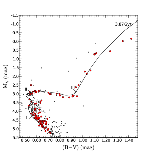
Figure 1: Color-magnitude diagram for M67 superposed upon the isochrone, which corresponds to an age of 3.87 Gyr. The red filled circles represent our work sample, i.e. stars with lithium abundance measurements. Stars with photometry available from Yadav et al. (2008), but with no lithium abundances, are displayed, for comparison with the isochrone, as black points. The squares represent the deviant stars. The roman numbers I, II, and III are described in Sect. 5.1 and correspond to the temperatures of, respectively, 6095, 6123, and 4966 K.

In Fig. 1, we plot a color-magnitude diagram of M67 stars, and the isochrone calculated from our models, with the parameters for M67 found in Castro et al. (2011), i.e. ${\rm[Fe/H]}=0.01$, $(m-M)=9.68$, and $E(B-V)=0.02$, and age of 3.87 Gyr. Black dots are the stars from the sample of Yadav et al. (2008), red filled circles are the stars studied in this paper, and open squares are deviant stars (see Sect. 5.3). Roman numbers I, II, and III are defined in Sect. 5.

Photometric and membership information, are available at CDS in electronic form (Table 1).

3 Temperatures and corrected lithium abundances

Lithium abundances are strongly sensitive to the effective temperature. To check for the dependence on the adopted effective temperatures, we compared different estimates, using the literature source from which the lithium abundances were also taken, a photometric calibration, and the isochrone. To determine the effective temperature by means of the isochrone, we proceeded in the following way: we plotted in the same CMD data points for each star and the isochrone computed for M67 age and metallicity, shifted according to its distance modulus and reddening. For each stellar data point, we then took the closest point on the isochrone, and adopted the corresponding physical parameters, i.e., in the case under consideration, effective temperature. For the remainder of the paper, we refer to this kind of temperature estimation as either “isochrone temperature”, or $T_{\rm iso}$ with the further specification of the isochrone used. “Isochrone masses” were computed in the very same way. Summarizing, we have the following four temperature estimations:

1. the $T_{\rm eff}$ adopted in the paper from which the lithium abundance was taken ($T_{\rm orig}$);

2. the isochrone temperature adopting models and parameters for M67 as in Yadav et al. (2008), who in turn adopted BaSTI models (Pietrinferni et al. 2004) ($T_{\rm iso-BaSTI}$);

3. the isochrone temperature adopting isochrones and parameters for M67 in Castro et al. (2011) ($T_{\rm iso-Castro}$);

4. using a photometric calibration, from Casagrande et al. (2010) for dwarfs and sub-giants, and from Kučinskas et al. (2005) for giants ($T_{\rm calib}$ or “calibration temperature”).

A comparison between the different temperature evaluations shows that the differences are significant. When comparing $T_{\rm orig}$ with the other temperature evaluations, the heterogeneity of the data, especially in the assumed reddening for M67, is certainly a main cause of these differences, and one of the aims of the present study is to homogenize the different determinations. The mean differences between $T_{orig}$ on the one hand, and $T_{\rm iso-BaSTI},T_{\rm iso-Castro}$, and $T_{\rm calib}$ on the other, are, respectively, 19, 50, and 95 K. The differences between calibration and isochrone temperatures arise, instead, from the isochrone in the CMD leaving most of the points on the right (cooler) side. This is because the calibration temperature is affected by the presence of undetected companions, which move the data points brighter and cooler in the CMD. In computing isochrone temperatures, we exploit the fact that the stars belong to the same cluster. The isochrone on the CMD is the locus where we would expect all the photometric data points to be if there were no photometric errors and no multiple systems. $T_{\rm iso}$ is the temperature corresponding to this locus, therefore it should be unaffected by the presence of undetected companions. This is confirmed by the overall good agreement between $T_{\rm iso}$ and $T_{\rm orig}$ for the 82 stars studied in Canto Martins et al. (2011), Castro et al. (2011), and Pasquini et al. (2008). In these stars, $T_{\rm orig}$ is based on spectroscopic analysis and is therefore very precise. We label $T_{\rm spec}$ this subset of $T_{\rm orig}$ based on spectroscopic analysis. The linear best fit to the data points in the $T_{\rm spec}$ versus isochrone temperature graph is very close to the identity: $T_{\rm iso-BaSTI}=0.99\cdot T_{\rm spec}-2.5$ K. We can confidently claim that the errors in the isochrone temperatures are random in nature.

We note that the two different evaluations of effective temperature using either isochrone, i.e. $T_{\rm iso-BaSTI}$ and $T_{\rm iso-Castro}$, are consistent with each other within the margins of error for most of the stars. The only significant differences arise for sub-giant stars and, to a lesser extent, for turn-off stars.

Corrections to lithium abundance measurements were applied according to the differences between $T_{\rm orig}$ and, respectively, $T_{\rm iso-BaSTI}$, $T_{\rm iso-Castro}$, and $T_{\rm calib}$. At the same time, we also took into account NLTE effects using the grid of NLTE corrections computed by Lind et al. (2009).

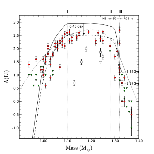
Figure 2: Lithium abundances as a function of stellar mass determined from the isochrone. Red filled circles represent stars with lithium abundance redetermined. The green triangles represent the lithium abundance upper limits. The open squares represents the deviant stars as discussed in Sect. 5.3. The continuous line corresponds to the lithium abundance predicted by our models with rotation-induced mixing calibrated for the Sun at the age of M67. The dashed line represents the same model shifted by 0.45 dex to match the observed lithium plateau. The dotted line represents models with rotation-induced mixing calibrated on the Hyades. The roman numbers I, II, and III are described in Sect. 5.1.

All temperature estimations, corrected and uncorrected lithium abundances, along with the photometric and membership information, are available on-line in Table 1.

In Fig. 2, we plotted the lithium abundances as a function of mass for both the stellar data points and two models. Red filled circles with error bars are the stars of our sample with detected lithium line, and green filled triangles represent upper limits. Open squares with error bars and, only in the case of one upper limit, the open triangle, represent the deviant stars discussed in Sect. 5.3. The models are discussed extensively in Sect. 4.

As mentioned above, Canto Martins et al. (2011), Castro et al. (2011), and Pasquini et al. (2008) computed temperature by carrying out a detailed spectroscopic analysis. Their temperature evaluation is more precise than that obtained using photometric information. Therefore, for the 82 stars studied in these works, we used the values given in the literature to produce Fig. 2. In contrast, for the remaining 21 stars, we used $T_{\rm iso-Castro}$, and the corresponding corrected value of the lithium abundance. For all of the stars, the mass adopted is the isochrone mass, which was computed using the isochrone and the parameters for M67 adopted in Castro et al. (2011).

4 Stellar evolutionary models

For this study, stellar evolutionary models were computed using the Toulouse-Geneva stellar evolution code TGEC (Hui-Bon-Hoa 2008). Details on the physics of these models can be found in Richard et al. (1996, 2004), do Nascimento et al. (2000), and Hui-Bon-Hoa (2008).

4.1 Input physics

We used the OPAL2001 equation of state by Rogers & Nayfonov (2002) and the radiative opacities by Iglesias & Rogers (1996), completed with the low temperature atomic and molecular opacities by Alexander & Ferguson (1994). The nuclear reactions were described by the analytical formulae of the NACRE (Angulo et al. 1999) compilation, taking into account the three pp chains and the CNO tricycle with the Bahcall & Pinsonneault (1992) screening routine. Convection was treated according to the Böhm-Vitense (1958) formalism of the mixing length theory with a mixing length parameter $\alpha=l/H_{\rm p}=1.74$, where $l$ is the mixing length and $H_{\rm p}$ the pressure height scale. For the atmosphere, we used a gray atmosphere following the Eddington relation, which is a good approximation for MS solar-type stars (VandenBerg et al. 2008).

The abundance variations in the following chemical species were computed individually in the stellar evolution code: H, He, C, N, O, Ne, and Mg. Both Li and Be were treated separately only as a fraction of the initial abundance. The heavier elements were gathered in a mean species Z. The initial composition follows the Grevesse & Noels (1993) mixture with an initial helium abundance $Y_{\rm ini}=0.268$. We chose to use the “old” abundances of Grevesse & Noels (1993) instead of the “new” mixture of Asplund et al. (2009). This choice was motivated by the disagreement between models computed with the new abundances and the helioseismic inversions for the sound-speed profile, the surface helium abundance, and the convective zone depth (e.g. Serenelli et al. 2009). Furthermore, according to Caffau et al. (2009), the solar metallicity using their own three-dimensional analysis is given by the values $Z=0.0156$ and $Z/X=0.0213$, which are closer to those of Grevesse & Noels (1993). In all cases, the solar abundances remain uncertain. We note that the accretion of metal-poor material (e.g. Castro et al. 2007; Guzik & Mussack 2010) as supported by the lack of refractory elements in the solar atmosphere (Meléndez et al. 2009), may help to reduce the discrepancy between the solar model and helioseismic data. Thus, the low solar abundances of Asplund et al. (2009) may actually be representative of the solar photosphere, while in the solar interior the abundances may be higher.

Diffusion and rotation-induced mixing.

The microscopic diffusion is computed with the atom test approximation. All models include gravitational settling with diffusion coefficients computed as in Paquette et al. (1986). Radiative accelerations are not computed here, since we focus only on solar-type stars where their effects are small when mixing is taken into account (Turcotte et al. 1998; Delahaye & Pinsonneault 2005). Rotation-induced mixing is computed as described in Théado & Vauclair (2003a). This prescription is an extension of the approach of Zahn (1992) and Maeder & Zahn (1998), and introduces the feedback effect of the $\mu$-currents in the meridional circulation, caused by the diffusion-induced molecular weight gradients. It introduces two free parameters in the computations: $C_{\rm h}$ and $\alpha_{\rm turb}$ (cf. Eq. (20) of Théado & Vauclair 2003a). The evolution in the rotation profile follows the Skumanich’s law (Skumanich 1972) with an initial surface rotation velocity on the zero-age main-sequence (ZAMS) equal to $V_{\rm i}=100$ km.s^-1, which roughly corresponds to the mean rotation velocity of stars hotter than about 7000 K in the Hyades according to the statistical study of Gaige (1993). The parameters of the Skumanich’s law are calibrated to match the solar rotation velocity at the solar age ($\sim 2\ \mathrm{km.s^{-1}}$). Other prescriptions were tested by other authors to model the lithium destruction. Charbonnel & Talon (1999) and Palacios et al. (2003) included angular momentum transport induced by mixing. However, since a rotation-induced mixing alone cannot account for the flat rotation profile inside the Sun, these authors later introduced the possible effect of internal gravity waves triggered at the bottom of the convective zone (see e.g. Talon & Charbonnel 2005), which allows the hot side of the Li-dip to be reproduced. Other authors suggested that the internal magnetic field is more important than internal waves in transporting angular momentum (Gough & McIntyre 1998). In any case, when applied to the solar case, all of these prescriptions are able to reproduce the lithium depletion observed in the Hyades, and the results are ultimately quite similar (Talon & Charbonnel 1998; Théado & Vauclair 2003b).

We also include a shear layer below the convective zone, which is treated as a tachocline (see Spiegel & Zahn 1992). This layer is parametrized with an effective diffusion coefficient that decreases exponentially downwards (Brun et al. 1998, 1999; Richard et al. 2004):

$$D_{\rm tacho}=D_{\rm bcz}\exp\left(\ln 2\frac{r-r_{\rm bcz}}{\Delta}\right)$$

where $D_{\rm bcz}$ and $r_{\rm bcz}$ are the value of $D_{\rm tacho}$ at the bottom of the convective zone and the radius at this location, respectively, and $\Delta$ is the half width of the tachocline. Both $D_{\rm bcz}$ and $\Delta$ are free parameters and the absolute size of the tachocline (i.e., $\Delta/R_{*}$ where $R_{*}$ is the radius of the star) is supposed to be constant during the evolution. An overshooting of parameter $\alpha_{\rm ov}=0.01H_{\rm P}$ has been included in the models that develop a convective core.

4.2 Models and calibration

We calibrated a model of 1.00 $\mathrm{M_{\odot}}$ to match the observed solar effective temperature and luminosity at the solar age. The calibration method of the models is based on the Richard et al. (1996) prescription: for a 1.00 $\mathrm{M_{\odot}}$ star, we adjusted the mixing-length parameter $\alpha$ and the initial helium abundance $Y_{\rm ini}$ to reproduce the observed solar luminosity and radius at the solar age. The observed values that we used are those of Richard et al. (2004), i.e., $L_{\odot}=3.8515\pm 0.0055\times 10^{33}$ erg.s^-1, $R_{\odot}=6.95749\pm 0.00241\times 10^{10}$ cm, and $t_{\odot}=4.57\pm 0.02$ Gyr. For the best-fit solar model, we obtained $L=3.8501\times 10^{33}$ erg.s^-1 and $R=6.95524\times 10^{10}$ cm at an age $t=4.576$ Gyr.

The free parameters of the rotation-induced mixing determine the efficiency of the turbulent motions. They are adjusted to produce a mixing that is both: 1) efficient and deep enough to smooth the diffusion-induced helium gradient below the surface convective zone, thus improving the agreement between the model and seismic sound speed profiles; 2) weak and shallow enough to avoid the destruction of Be. Following Grevesse & Sauval (1998), the Be abundance of the Sun is $A({\rm Be})=1.40\pm 0.09$. We obtained a slight Be destruction by a factor of 1.33 with respect to the meteoritic value, which is well within the error in the solar Be abundance.

The calibration of the tachocline allows us to reach the solar lithium depletion ($A({\rm Li})=1.10\pm 0.10$ (e.g. Grevesse & Sauval 1998) and for our best-fit solar model we obtained $A({\rm Li})=1.04$. We also checked that the sound velocity profile of our best-fit model is consistent with that deduced from helioseismology inversions by Basu et al. (1997). Our calibration is in excellent agreement with helioseismology, more accurately than 1% for most of the star, except in the deep interior, where the discrepancy reaches 1.5%.

We computed a grid of evolutionary models of masses in the 0.90 to 1.34 $\mathrm{M_{\odot}}$  range, with a step of 0.01 $\mathrm{M_{\odot}}$  in mass, and a metallicity of ${\rm[Fe/H]}=0.01$, which is a simple average of different estimates of the metallicity of M67 (see Pasquini et al. 2008). We ran the models from the ZAMS to the top of the RGB for the most massive stars. The input parameters for all the models are the same as for the 1.00 $\mathrm{M_{\odot}}$ model.

There is no a priori reason why the calibration of the parameters of the extra mixing for the model of 1.00 $\mathrm{M_{\odot}}$ should also hold for different masses, and at different times during the evolution of the stars. In their work, Théado & Vauclair (2003b) adjusted the free parameters of the rotation-induced mixing with the TGEC for each one of the models of different masses to obtain the correct lithium depletion at the age of the Hyades. They noted that the horizontal diffusion coefficient is very mass-dependent. The uncertainty associated with these parameters led us to analyze their impact on the destruction of lithium as a function of stellar mass. To do so, a first set of models was calculated to reproduce the profile of lithium abundance as a function of mass for the Hyades open cluster. Our Hyades sample is a compilation of EW measurements of the lithium line at 6708 AA from several sources (Randich et al. 2007; Thorburn et al. 1993; Soderblom et al. 1990; Boesgaard & Budge 1988; Boesgaard & Tripicco 1986; Duncan & Jones 1983; Rebolo & Beckman 1988). All the stars identified as binaries in Thorburn et al. (1993) were excluded. When more than one reference was available for a star, we used the most recent. Masses and temperatures were taken either directly from Balachandran (1995), or computed from the relationship between B-V and, respectively, mass and temperature, obtained from the data in the same paper. The result of the compilation is available at CDS in electronic form (Table 2). The parameters $C_{\mathrm{h}}$ and $\alpha_{\mathrm{turb}}$ of the rotation-induced mixing of the models, with masses from 0.800 to 1.400 $\mathrm{M_{\odot}}$, with a step of 0.050 $\mathrm{M_{\odot}}$, are calibrated to reproduce at the age of the Hyades (625 Myr) the observed destruction of lithium. In these calibrations, we did not include the tachocline that is used in the code to calibrate solar models, because in the solar mass stars the bottom of the convective zone is very close to the lithium destruction layer (Théado & Vauclair 2003b). The same calibration is then used to calculate a set of models of M67 stars. The values of the parameters $C_{\mathrm{h}}$ and $\alpha_{\mathrm{turb}}$ for all calibrations are given in Table 3.

Table 3: Parameters of the rotation-induced mixing in TGEC models.

Calibration	Mass ($\mathrm{M_{\odot}}$)	$C_{\mathrm{h}}$	$\alpha_{\mathrm{turb}}$
Sun	1.000	9000	1.00
	0.800	3400	4.00
	0.850	10000	5.00
	0.900	10000	5.50
	0.950	10000	5.60
	1.000	10000	5.15
	1.050	7000	4.25
Hyades	1.100	5000	3.30
	1.150	4500	2.50
	1.200	2500	2.10
	1.250	2546	2.15
	1.300	2600	2.75
	1.350	6500	3.50
	1.400	10000	4.50

5 Discussion

The observed spread in the lithium abundance versus mass distribution of M67 for stars of about one solar mass or lower, which can be clearly seen in Fig. 2, suggests that an extra variable (in addition to mass, age, and metallicity) is at work, leading to different lithium depletion in cluster stars of the same mass. The fundamental question here (since the spread is present) is which other variable may cause a large range of lithium abundance at a fixed mass?

Our database includes stars ranging from the MS to the sub-giant and giant branches, so is well-suited to both address the issue of spread and test models of non-standard mixing for different masses.

Models that point to rotational mixing as the major cause of lithium depletion (see e.g. Pinsonneault 2010, for a review), predict that this only depends on the age, metallicity, mass, and the initial angular momentum of the star. This last parameter, however, may vary for otherwise similar stars, introducing a spread in the lithium abundances. The variation in the initial rotation velocity by a factor two in our models has a weak effect of about 0.05 dex of magnitude for the lithium destruction, because the Skumanich’s law used implies that there is a strong drop in the rotation velocity very early on in stellar evolution. The Skumanich’s law is empirical, and we should in the future include in the code the transport of angular momentum to ensure a more reliable estimation of the spread of the lithium abundance due to a possible spread in the initial angular momentum.

The depth of the surface convection zone and the nuclear burning depend strongly on the total stellar mass (do Nascimento et al. 2009), thus the most appropriate way to investigate the abundance of lithium in these M67 stars is first to divide our sample of stars in three different groups of mass range. MS stars with $M\leq$ 1.1 $\mathrm{M_{\odot}}$, stars close to the turnoff with 1.1 $\mathrm{M_{\odot}}$$<M\leq$ 1.28 $\mathrm{M_{\odot}}$, and evolved sub-giant and giant stars with $M>$1.28 $\mathrm{M_{\odot}}$.

5.1 Lithium abundance and mass

In Fig. 2, we compare our model predictions with our inferred stellar masses and lithium abundances for our sample of M67 stars. The solid line represents an isochrone constructed with all the models including the effects of atomic diffusion, gravitational settling, and rotation-induced mixing calibrated for the Sun as described in Sect. 4. The age of the models is 3.87 Gyr as determined in Castro et al. (2011). Initial lithium abundances were chosen to equal $A({\rm Li})=3.26$, the estimated initial solar value based on meteorites (Asplund et al. 2009). This lithium abundance is 0.05 dex lower than the previously accepted meteoritic lithium abundance ($A({\rm Li})=3.31$, see Grevesse & Sauval 1998). The dashed line represents an isochrone for the same models but where the initial lithium abundance was rescaled by $-$0.45 dex to fit the plateau at $A({\rm Li})=2.5$. This suggests that the initial M67 lithium abundance may have been lower than 3.26, or that our models are not depleting enough lithium. We note, however, that according to Deliyannis et al. (1994), based on a short-period tidally locked binary in M67, the initial lithium abundance in M67 was at least $A({\rm Li})=3.0$. This would reduce the shift necessary to match our models with the lithium content in the plateau to only about $-$0.2 dex. However, the hypothesis of a lower initial lithium content seems weak and unrealistic. We are left with an insufficient destruction of lithium by rotationally driven mixing mechanisms. Théado & Vauclair (2003b) showed that for masses higher than 1.0 $\mathrm{M_{\odot}}$, it is necessary to increase the values of these parameters as a function of mass to account for the lithium depletion at the age of the Hyades. To analyze the influence of these parameters on the lithium destruction, we calculated another set of models, in which the rotation-induced mixing parameters was calibrated for each mass, as described in Sect. 4. The isochrone at the age of M67 of these models is represented by the dotted line in Fig. 2. These models reproduce more closely in a quantitative way the profile of lithium destruction in M67, but the arbitrary calibration of the mixing parameters for each mass is a very unsatisfactory method. There appears to be no clear relation between the mixing parameters and mass that might have a physical significance.

For stars with masses lower than 1.1 $\mathrm{M_{\odot}}$ (roman number I in Fig. 1 and Fig. 2), the lithium depletion progressively increases toward lower masses. A dispersion is observed in this mass range and confirmed by several authors (Pasquini et al. 1997; Jones et al. 1999; Randich et al. 2002, 2007; Pasquini et al. 2008). We note that in this region, some upper limits used may be considered as too optimistic. In this context, Önehag et al. (2011) analyzed the M67 solar twin YBP 1194 using spectra of good quality ($R\sim 50,000,S/N=160$), but even with such a spectrum they found that it is challenging to robustly determine a lithium abundance in the solar twin YBP 1194. A careful analysis of solar analogs in M67 using high quality spectra is urgently needed for stars around 1 $\mathrm{M_{\odot}}$. However, we note that four stars at 1.01 $\mathrm{M_{\odot}}$ span as wide a range of lithium abundances as 1.1 dex, and one of them is a revised upper limit. A considerable amount of scatter in the data in this region remains after raising the upper limits, whose real presence should be considered highly probable based on the presently available data. Stellar rotation and the history of angular momentum induce it either directly through rotational mixing or indirectly by driving other processes such as diffusion and internal gravity waves (Montalbán & Schatzman 2000). Planetary accretion may also be at work in solar-type stars, and induce mass-independent lithium destruction (Théado et al. 2010).

The low lithium abundance observed in low-mass stars in M67 also exists because these stars have had more time to burn their lithium during the PMS and have a surface convection zone that both retreats more slowly and ends up at greater depths on the MS. We note that, for this range of masses and these evolutionary stages, the standard models predict that the bottom of the convective zone is not hot enough to account for the decrease in lithium, even though the observed low lithium abundances clearly indicates the need for a more realistic representation of transport mechanisms in low mass stars.

Stars with masses 1.1 $\mathrm{M_{\odot}}$$<M\leq$ 1.28 $\mathrm{M_{\odot}}$ (between roman number I and II in Figs. 1 and 2) are close to the turn off (or about to leave the MS) and at these masses the surface convection zone and the mixed layers below the convection zone are too thin to support temperatures high enough to cause the nuclear destruction of lithium. Furthermore in this mass range the PMS lithium depletion tapers off to essentially zero. We can therefore easily see why there should be a plateau with a nearly constant lithium abundance for this mass range. One important test of our model will be in fact to reproduce the general morphology of the lithium depletion behavior.

This is the region where the offset between our models and observations becomes apparent, as discussed above.

Stars with masses above 1.28 $\mathrm{M_{\odot}}$ are sub-giants following an evolutionary path from the turn-off to the RGB. In Figs. 1 and 2, this stage is marked by the roman numbers II and III. The lithium abundance predicted for standard models of sub-giant and giant stars is mainly controlled by dilution (Iben 1966, 1967a, 1967b; Scalo & Miller 1980). This process was described originally by Iben (1965) and appears when a star evolves off the MS. When the stars crosses the sub-giant branch and climbs the RGB, the surface convective zone increases its fraction in mass. Lithium-poor material rises to the surface and is mixed with Li-rich material. This process stops when the convective zone reaches its maximum size. From our models, the predicted value for lithium-abundance post-dilution is $A({\rm Li})=1.0$ dex. The observations clearly show the need for a non-standard transport processes for sub-giants and evolved stars of M67. Canto Martins et al. (2011) discussed the depletion of the surface lithium abundance and whether there is an additional non-standard transport process related to the transport of matter and angular momentum by meridional circulation and shear-induced turbulence (Ryan & Deliyannis 1995).

5.2 Prediction by other models

Our models successfully reproduce qualitatively the lithium depletion seen in different mass regimes in M67 stars, as shown in Fig. 2. In Fig. 3, the evolution with age at different masses is shown. We note that fully independent non-standard models by Xiong & Deng (2009), also show similar trends between lithium depletion, mass, and age.

As shown in Fig. 1 of Xiong & Deng (2009), at 4 Gyr, there is a large depletion in the lithium for models of 1 $\mathrm{M_{\odot}}$. As in our models, the less depleted stars are those with masses somewhat higher than 1.1 $\mathrm{M_{\odot}}$, although the Xiong & Deng (2009) model also fails to predict exactly the peak or plateau in lithium abundance for M67 stars close to the turnoff, requiring probably an additional lithium depletion of 0.3 dex. Stars with masses higher than 1.3 $\mathrm{M_{\odot}}$ show severe depletion at 4 Gyr, probably because they should be in the sub-giant or giant phase. Thus, qualitatively, the models by Xiong & Deng (2009) also reproduce the M67 observations.

5.3 Deviant stars

Although overall lithium abundance appears to be a tight function of mass for stars more massive than 1.06 $\mathrm{M_{\odot}}$, a few objects dramatically depart from the general trend.

These objects are marked by open square symbols in Figs. 1 and 2, and are discussed below.

YBP 1075, YBP 750, YBP 769: These objects, despite being quite distant from the isochrone in the CMD diagram (more than 0.1 mag, limit under which 80% of the sample lies), are all secure members (99 or 100% of probability, based also on radial velocity). They are therefore likely to have companions too small to be detected, but bright enough to affect color and brightness. Their lithium abundance deficiency, with respect to the mean trend with the mass, is about 2.3, 1.0, and 0.5, dex respectively, much more than errors can possibly explain, and they have estimated masses in the narrow range between 1.12 and 1.18 $\mathrm{M_{\odot}}$. Therefore, the question of whether we identify a “secondary dip” is legitimate, although strong caution should be exercised before claiming it as highly probable. Their mass range encompasses four more stars, three of which lie significantly closer to the isochrone. If we formulate the intriguing hypothesis of an extra-mixing mechanism triggered in this narrow mass range by a low mass companion, we are still left with the unexplained case of YBP 1680, which is also likely to have a small undetected companion, but does not show any anomaly as far as lithium abundance is concerned. This matter deserves further attention.

YBP 890: This star is also a secure member, but, contrary to the three discussed above, its distance to the isochrone in the CMD is only 0.03 mag. It has a mass of about 1.24 $\mathrm{M_{\odot}}$, and a lithium abundance about 0.9 dex lower than YBP 961, which is estimated to be at about the same mass. Its lithium abundance is an upper limit, it may therefore be more peculiar than it appears. This star has undoubtly undergone a strong amount of extra mixing.

YBP 871 and YBP 778 are also significantly under-abundant in lithium, and have masses similar to that of YBP 890. Their distance to the isochrone in the CMD is about 0.06 mag, which is larger than for YBP 890 but not dramatically large. In their case, however, we still cannot completely rule out the possibility of a combination of errors in the abundance and mass to explain their peculiar position in Fig. 2.

YBP 942: This is a secure member of the cluster, the only star with a peculiarly high lithium abundance, which is 0.5 and 0.8 dex higher than the slightly less massive stars YBP 1320 and YBP 1318. Rather than an error in the abundance, an overestimation of the mass of this star of about 0.05 $\mathrm{M_{\odot}}$ could help us to explain its abundance anomaly. However, its distance from the isochrone in the CMD is large at about 0.1 mag.

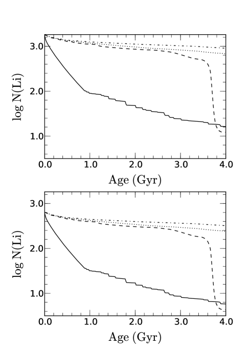
Figure 3: Lithium abundance predicted by our models as a function of time for different masses. Upper panel: for a MS star with M = 1 $\mathrm{M_{\odot}}$(solid line), stars of M = 1.15 $\mathrm{M_{\odot}}$(dot-dashed) and 1.28 $\mathrm{M_{\odot}}$(dotted) currently around the turn-off, and a more massive star of 1.33 $\mathrm{M_{\odot}}$(dashed line) that is already a giant. Lower panel: same plot, but after a -0.45 dex shift was applied (as in Fig. 2).

5.4 Lithium abundance, rotation, and chromospheric activity in M67

In stars with a convective envelope, the chromosphere and chromospheric activity are generated by non-radiative heating mechanisms caused by a magnetic field (see e.g. Hall 2008, for a review). Rotation and differential rotation play a key role in this process, because they are at the base of the dynamo effect that sustain magnetic activity (Böhm-Vitense 2007). Magnetic braking spins down the star, which therefore loses chromospheric activity as it loses angular momentum. While until a few years ago there was general consensus that chromospheric activity decays smoothly during the whole stellar life-time (e.g. Skumanich 1972; Barry et al. 1987; Soderblom et al. 1991; Donahue 1998; Lachaume et al. 1999), which is still widely accepted (Mamajek & Hillenbrand 2008), alternative views have also been expressed later on (Pace et al. 2009; Lyra & Porto de Mello 2005; Zhao et al. 2011). However, nobody questions that young stars are more chromospherically active than stars older than 1.5 Gyr (Soderblom 2010).

This picture suggests that chromospheric activity may be related to rotation and age, in a very similar way as lithium abundance. This is the rationale for a comparison between these three parameters in M67.

Figure 4: On the left: chromospheric activity as a function of mass. On the right: lithium abundances versus chromospheric activity. Empty circles around filled symbols indicate the stars with measured projected rotation velocity. Among these measurements, only that of YBP 1067 exceeds 2  $\mathrm{km\,s^{-1}}$, and it is of 4  $\mathrm{km\,s^{-1}}$.

The most extensive chromospheric-activity survey made in M67 is that by Giampapa et al. (2006), who collected data for over 60 MS stars. They used the HK index, i.e. a measure of the strength of the chromospheric emission in the core of the Ca II H and K line, in mÅ. The HK index is neither transformed into flux, nor corrected for photospheric contribution. Mamajek & Hillenbrand (2008) transformed the HK indices of Giampapa et al. into $R^{\prime}_{\rm HK}$, i.e. they subtracted the photospheric contribution, transformed it into flux, and normalized it for the bolometric emission. The data were taken over a time span of five years, and measurements for each star were time-averaged over large part of this interval, which is of crucial importance since the chromospheric activity undergoes a short-term variation analog of the 11-year solar cycle. Thirty-five stars studied by Giampapa et al. have published lithium abundances that are collected here and plotted in Fig. 4. In this figure, we show the HK index in mÅ as a function of mass (Left panel) and HK index versus lithium abundances (Right panel). Here upper limits are indicated as downward arrows. Circles surrounding the dots indicate that the star has a rotation velocity measurement available (see below). The left panel has the purpose of identifying the two active outliers. It is similar to Fig. 4 in Giampapa et al., in which B-V color is a substitute for mass, but we note that among the two active stars in both figures, the only star in common is Sanders 1050/YBP 1342. The star Sanders 747/YBP 681 is given in Fig. 4 of Giampapa et al. and not in our Fig. 4 because it is a binary, and we excluded it from our compilation. On the contrary, we plot Sanders 1452/YBP 1067, which is outside the margins of Fig. 4 of Giampapa et al.. In the right panel, we show that the two active outliers are highly lithium-depleted. However, these high levels of lithium depletion are also found in many other inactive stars. The Pearson correlation coefficient between the HK index and the lithium abundance is weak but significant at $-$0.25. This weak correlation cannot be an effect of a correlation between HK index and mass, which, for our sample, are completely unrelated. However, the correlation between HK index and lithium abundance is entirely due to the two chromospherically active and highly lithium depleted stars. If we remove them, the correlation between HK and lithium abundance is $-$0.05, which corresponds to a probability of the two quantities being unrelated of about 80%.

Reiners & Giampapa (2009) measured the projected rotation velocities of 15 stars selected from the sample of Giampapa et al. in order to check whether rotation was at the base of the higher chromospheric activity level of some stars. The measurements were based on the cross-correlation profile of high-resolution spectra. Nine of these stars are present in our compilation of lithium abundances, and are indicated in Fig. 4 with a circle surrounding the dot. With the only exception of YBP 1067, all of the projected rotation velocities are consistent with the solar rotation, as they have an upper limit of about 2  $\mathrm{km\,s^{-1}}$. On the contrary, YBP 1067 has a projected rotation velocity of about 4  $\mathrm{km\,s^{-1}}$, i.e. it rotates at least twice as fast as the sun. Whether this suggests a relationship between rotation and lithium abundance is unclear. On the one hand, YBP 1067 has a very low lithium abundance, on the other hand there are two slow rotators with an even lower lithium content and one more slow rotator with an upper limit only slightly above the lithium abundance measurement for YBP 1067. More data are warranted to shed light on this matter. In particular, it would be very important to obtain true rotation periods instead of only $v$ sin $i$.

6 Conclusions

Spectroscopic observations of stars in the open cluster M67 provide important constraints to test non-standard models of lithium depletion. We have rederived the effective temperatures of M67 stars and corrected the lithium abundances available in the literature, in order to have a homogeneous data-set for comparison with our models. We have also taken into account NLTE effects, providing a homogeneous set of NLTE Li abundances in M67. Tables with our $T_{\rm eff}$, NLTE lithium abundances, and masses are presented, so that other groups can test their non-standard stellar models.

M67 stars close to the turn-off, with masses $M=1.1-1.28$ $\mathrm{M_{\odot}}$, have a peak or a plateau in lithium abundances. Less massive stars ($M<1.1$ $\mathrm{M_{\odot}}$) display strong lithium depletion, which increases for lower masses owing to a deepening of their convection zones. Evolved sub-giant and giant stars with $M>1.28$ $\mathrm{M_{\odot}}$  show lower Li abundances due to a dilution of their original lithium content. The above pattern is qualitatively well-reproduced by our models, as well as by the independent models of Xiong & Deng (2009).

The lithium abundance appears to be a tight function of the mass, for stars more massive than the Sun, with a few notable exceptions that deserve a closer look. In particular, based on three over-depleted stars, we suggest that, at about 1.15 $\mathrm{M_{\odot}}$, the presence of a small companion may trigger a large amount of extra mixing, or perhaps the initial rotation velocity was higher in these stars. More observations are needed before drawing firm conclusions about these outliers.

Our models qualitatively reproduce many observed features of the lithium abundance as a function of mass. However, we are still far from achieving a close match between observations and models with a unique combination of the parameters.

Two stars in our compilation have chromospheric activity levels that are unusually high. They are both highly lithium depleted but, apart from this circumstance, no strong relationship between chromospheric activity and lithium abundance seems to be present. Only for one of the two chromospherically active stars has a projected rotation velocity been measured, which is $\sim 4$  $\mathrm{km\,s^{-1}}$, the only value that exceeds 2  $\mathrm{km\,s^{-1}}$  among the nine measurements in our sample. This suggests that rotation is at the base of both lithium depletion and higher chromospheric activity in this star, but that other extra mixing processes must also be efficient in some slow rotators.

Table 4: M67 data. See Sects. 2 and 3 for explanations.

star	V	B-V	pmb	vrad	ref	Aorig	Torig	Aiso-Castro	Tiso-Castro	Acalib	Tcalib	$\Delta$ A
	(mag)	(mag)	$\%$	( $\mathrm{km\,s^{-1}}$)		(dex)	(K)	(dex)	(K)	(dex)	(K)	dex
Sand. 774	12.93	0.85	–	33.5	1	0.0	5240	0.16	5176	0.13	5253	up.lim.
YBP 1632	12.734	0.795	100	33.4	1	0.0	5461	0.17	5260	0.12	5398	0.2
Sand. 978	9.72	1.37	–	34.7	1	-1.0	4260	-0.73	4325	-0.71	4283	0.3
YBP 1087	10.413	1.139	98	33.9	1	0.0	4748	0.06	4518	0.12	4623	up.lim.
Sand. 1016	10.3	1.26	–	34.6	1	-0.5	4430	-0.16	4487	-0.2	4432	0.2
YBP 1248	12.639	0.615	99	34.6	1	1.3	6020	1.38	6109	1.26	5937	0.1
YBP 1479	10.462	1.127	97	34.2	1	-0.4	4750	-0.14	4528	-0.15	4644	0.2
YBP 829	12.891	0.935	100	32.9	1	0.1	5130	0.24	5128	0.25	5029	up.lim.
YBP 923	12.753	0.744	100	32.719	1	0.8	5644	0.57	5284	0.82	5541	up.lim.
YBP 942	12.678	0.723	99	37.972	1	2.7	5810	2.36	5395	2.54	5601	0.1
YBP 973	12.944	0.904	99	33.009	1	0.0	5170	0.14	5176	0.15	5121	0.2
YBP 1060	11.465	1.04	97	32.9	1	-0.4	4820	-0.19	4742	-0.2	4801	up.lim.
YBP 1258	12.616	0.587	99	32.7	1	0.9	5996	1.04	6081	1.03	6031	0.1
YBP 1318	12.238	0.572	98	34.641	1	1.9	6159	1.74	5929	1.85	6082	0.1
YBP 1320	12.579	0.606	99	34.322	1	2.2	6050	2.2	6039	2.15	5967	0.1
YBP 1327	11.598	1.057	98	34.6	1	-0.4	4820	-0.21	4775	-0.18	4769	up.lim.
YBP 1362	10.492	1.122	97	33.65	1	-0.5	4779	-0.19	4539	-0.22	4652	0.2
YBP 1546	12.245	0.986	96	33.978	1	-0.2	4940	-0.04	4909	-0.04	4910	up.lim.
YBP 1777	12.87	0.932	99	34.4	1	0.4	5104	0.55	5128	0.52	5037	up.lim.
YBP 1844	12.764	0.736	91	33.2	1	1.0	5654	0.74	5284	0.99	5564	up.lim.
YBP 846	12.838	0.824	100	33.1	1	0.0	5420	0.2	5176	0.16	5321	up.lim.
YBP 1876	12.577	0.641	99	33.921	1	1.1	5940	0.96	5727	1.06	5852	0.1
Sand. 1607	12.62	0.56	–	33.7	1	1.7	6127	1.69	6095	1.71	6124	0.1
YBP 1070	12.631	0.62	100	33.637	1	1.2	6000	1.29	6095	1.16	5920	0.1
YBP 1086	12.752	0.821	100	33.0	1	0.7	5429	0.62	5223	0.7	5329	0.1
YBP 285	14.461	0.704	98	33.951	2	0.6	5836	0.63	5767	0.64	5657	0.1
YBP 637	14.489	0.702	99	34.241	2	1.5	5806	1.5	5754	1.43	5663	0.1
YBP 1101	14.675	0.702	99	32.927	2	0.6	5756	0.63	5649	0.64	5663	up.lim.
YBP 1194	14.614	0.667	99	33.673	2	1.3	5766	1.29	5688	1.35	5770	up.lim.
YBP 1303	14.641	0.677	99	33.241	2	1.2	5716	1.22	5675	1.27	5739	0.1
YBP 1304	14.731	0.723	99	33.696	2	0.8	5704	0.82	5623	0.8	5601	up.lim.
YBP 1315	14.297	0.693	99	32.434	2	1.8	5874	1.82	5861	1.69	5691	0.1
YBP 1392	14.811	0.716	97	34.171	2	0.6	5716	0.65	5584	0.65	5622	up.lim.
YBP 1787	14.547	0.667	98	33.386	2	1.6	5768	1.61	5727	1.65	5770	0.1
YBP 2018	14.565	0.672	98	31.74	2	1.3	5693	1.37	5714	1.4	5755	up.lim.
YBP 266	13.601	0.611	100	33.392	3	2.5	6147	2.5	6151	2.36	5950	0.1
YBP 288	13.857	0.637	99	32.796	3	2.3	6004	2.34	6067	2.2	5865	0.1
YBP 349	14.301	0.677	93	34.132	3	1.0	5952	0.94	5861	0.86	5739	up.lim.
YBP 350	13.624	0.602	99	32.778	3	2.6	6024	2.68	6137	2.57	5980	0.1
YBP 401	13.661	0.607	97	32.917	3	2.4	6165	2.38	6137	2.26	5963	0.1
YBP 473	14.443	0.699	99	35.269	3	1.0	5919	0.91	5780	0.85	5672	up.lim.
YBP 587	14.107	0.646	99	33.265	3	2.3	6077	2.21	5956	2.12	5836	0.1
YBP 613	13.254	0.653	99	33.274	3	2.6	6202	2.53	6095	2.32	5814	0.1
YBP 673	14.356	0.706	99	32.902	3	1.4	5639	1.55	5834	1.41	5652	0.1
YBP 689	13.12	0.663	99	33.461	3	2.3	6093	2.26	6039	2.07	5783	0.1
YBP 750	13.576	0.639	100	33.709	3	1.5	5918	1.67	6151	1.45	5859	0.1
YBP 769	13.478	0.641	100	34.414	3	2.0	5984	2.12	6151	1.9	5852	0.1
YBP 778	13.093	0.623	99	33.815	3	1.7	6114	1.65	6039	1.55	5911	0.1
YBP 809	14.959	0.737	97	32.948	3	1.0	5667	0.86	5495	0.92	5561	up.lim.
YBP 851	14.113	0.617	98	34.204	3	1.3	5948	1.31	5956	1.29	5930	0.1
YBP 911	14.547	0.673	99	32.534	3	1.2	5885	1.08	5727	1.1	5752	0.1
YBP 988	14.18	0.639	99	32.705	3	2.0	5935	2.0	5929	1.94	5859	0.1
YBP 1032	14.358	0.639	97	34.302	3	1.6	5955	1.51	5834	1.53	5859	0.1
YBP 1036	14.947	0.731	98	33.884	3	1.4	5612	1.31	5495	1.37	5578	0.1
YBP 1051	14.09	0.636	99	32.029	3	2.2	6081	2.12	5970	2.04	5868	0.1
YBP 1062	14.477	0.667	99	33.206	3	1.7	5926	1.58	5767	1.58	5770	0.1
YBP 1067	14.559	0.642	100	34.67	3	1.0	5929	0.87	5727	0.94	5849	0.1
YBP 1075	13.712	0.674	99	32.974	3	0.7	5871	0.94	6123	0.69	5749	0.1
YBP 1088	14.492	0.659	93	33.199	3	1.0	5890	0.91	5754	0.93	5795	up.lim.
YBP 1090	13.8	0.65	100	32.333	3	2.3	6086	2.31	6095	2.11	5824	0.1
YBP 1129	14.171	0.624	99	34.528	3	2.1	5959	2.09	5942	2.06	5907	0.1
YBP 1137	14.873	0.698	97	33.851	3	1.0	5741	0.87	5546	0.95	5675	up.lim.
YBP 1197	13.315	0.606	100	34.526	3	2.2	6207	2.14	6123	2.03	5967	0.1
YBP 1247	14.144	0.609	99	32.991	3	2.1	5994	2.06	5942	2.07	5957	0.1
YBP 1334	14.403	0.68	99	32.923	3	2.0	5957	1.89	5807	1.82	5730	0.1
YBP 1387	14.098	0.626	99	33.828	3	2.3	6090	2.22	5970	2.16	5901	0.1
YBP 1458	14.977	0.739	98	33.351	3	1.0	5640	0.87	5482	0.94	5555	up.lim.
YBP 1496	13.879	0.607	100	34.607	3	2.6	6173	2.52	6053	2.45	5963	0.1
YBP 1504	14.171	0.625	99	33.733	3	2.2	5934	2.21	5942	2.18	5904	0.1
YBP 1514	14.777	0.721	98	33.878	3	1.6	5613	1.59	5597	1.6	5607	0.1
YBP 1587	14.163	0.641	99	32.336	3	2.0	5975	1.98	5942	1.91	5852	0.1
YBP 1622	14.156	0.632	99	33.407	3	2.2	6043	2.13	5942	2.08	5881	0.1
YBP 1716	13.299	0.619	96	33.948	3	2.3	6030	2.36	6123	2.22	5924	0.1
YBP 1722	14.13	0.601	96	34.007	3	2.2	6007	2.16	5956	2.18	5983	0.1
YBP 1735	14.332	0.661	97	33.104	3	0.9	5959	0.83	5847	0.81	5789	0.1
YBP 1758	13.207	0.653	98	34.398	3	2.4	6221	2.29	6067	2.11	5814	0.1
YBP 1768	14.404	0.656	99	34.222	3	2.1	5844	2.07	5807	2.07	5805	0.1
YBP 1788	14.441	0.663	84	33.763	3	1.8	5886	1.72	5780	1.72	5783	0.1
YBP 1852	13.962	0.613	99	32.324	3	2.1	6009	2.11	6025	2.05	5943	0.1
YBP 1903	14.733	0.689	99	32.409	3	1.0	5609	1.01	5623	1.07	5703	up.lim.
YBP 1948	14.015	0.612	97	33.136	3	2.4	6164	2.29	5997	2.25	5947	0.1
YBP 1955	14.212	0.63	98	32.588	3	2.2	5961	2.17	5915	2.14	5888	0.1
YBP 901	13.422	0.554	100	–	4	2.63	6191	2.57	6137	2.58	6145	0.07
YBP 963	12.76	0.565	100	–	4	2.1	6210	2.09	6194	2.03	6106	0.08
Sand. 998	13.06	0.558	–	–	4	2.64	6223	2.5	6053	2.56	6131	0.06
YBP 871	13.152	0.582	100	–	4	1.86	6156	1.79	6053	1.79	6048	0.16
Sand. 1064	14.04	0.661	–	32.7	5	2.14	5845	2.28	5997	2.12	5789	0.1
YBP 713	14.172	0.714	99	35.443	5	2.07	5800	2.2	5929	1.97	5628	0.1
YBP 1105	13.946	0.59	99	32.8	5	2.55	6094	2.5	6039	2.49	6020	0.1
YBP 1397	14.009	0.622	97	36.808	5	2.28	5972	2.32	6011	2.25	5914	0.1
YBP 1342	14.285	0.65	99	33.684	5	1.15	5810	1.24	5874	1.2	5824	up.lim.
Sand. 1057	14.3	0.668	–	34.5	5	1.75	5818	1.82	5861	1.75	5767	0.1
YBP 1486	13.864	0.574	94	–	6	2.63	6178	2.54	6067	2.54	6075	0.1
YBP 890	13.179	0.59	100	34.212	6	1.48	6153	1.43	6067	1.4	6020	up.lim.
YBP 961	13.19	0.576	100	34.59	6	2.37	6151	2.31	6067	2.31	6068	0.1
YBP 1680	13.646	0.645	100	35.428	6	2.45	5934	2.6	6137	2.38	5840	0.1
Sand. 1055	13.8	0.593	–	–	6	2.43	6116	2.41	6095	2.35	6010	0.1
YBP 1456	12.841	0.943	100	–	7	0.5	5000	0.75	5105	0.67	5008	up.lim.
YBP 877	12.732	0.583	99	–	7	1.9	6205	1.89	6194	1.79	6044	up.lim.
YBP 891	11.401	1.089	98	–	7	0.0	4740	0.2	4731	0.18	4710	up.lim.
YBP 1017	12.361	0.962	96	33.639	7	0.5	4905	0.7	4931	0.74	4962	up.lim.
YBP 1024	9.586	1.443	98	31.655	7	-1.0	4010	-1.01	4295	-0.83	4176	up.lim.
YBP 1337	12.878	0.972	100	–	7	0.9	4850	1.35	5105	1.18	4940	0.1
References:
(1) Canto Martins et al., 2011, A&A 527, A94;
(2) Castro et al., 2011, A&A 526, 17;
(3) Pasquini et al., 2008, A&A 489, 677;
(4) Randich et al. 2007, A&A 469, 163;
(5) Jones, Fischer and Soderblom 1999, ApJ 117, 330, original data;
(6) Jones, Fischer and Soderblom 1999, ApJ 117, 330, correction of literature measurements;
(7) Balachandran 1995, Apj 446, 203.

Table 5: Hyades data

vB	V	B-V	$T_{\rm eff}$	log g	Mass	EW	$\Delta$EW	A(Li)	$\Delta$ A	EW ref	phot ref
2	7.78	0.617	5916	4.36	1.140	89.0	2	2.73	0.03	T	Bal.
3	8.88	0.848	5099	4.48	0.847	$\leq$25.0		$\leq$ 1.37		D	Bal.
4	5.97	0.341	6897	3.99	1.524	$\leq$3.0		$\leq$ 1.79		T	Bal.
6	5.95	0.348	6861	3.96	1.513	54.8	3	3.10	0.04	BB	Joner
8	6.37	0.419	6544	4.02	1.411	$\leq$4.0		$\leq$ 1.69		BB	Bal.
10	7.85	0.589	6000	4.42	1.182	82.0	2	2.74	0.03	T	Bal.
13	6.62	0.420	6542	4.12	1.410	$\leq$5.0		$\leq$ 1.79		BT	Bal.
14	5.73	0.355	6825	3.87	1.502	65.0	3	3.18	0.04	BT	Bal.
15	8.09	0.658	5703	4.39	1.037	57.0	2	2.32	0.03	T	Bal.
17	8.46	0.696	5539	4.47	0.971	42.0	2	2.03	0.05	T	Bal.
18	8.06	0.638	5779	4.41	1.072	74.0	2	2.52	0.04	T	Bal.
19	7.14	0.512	6231	4.22	1.290	82.4	3	2.91	0.03	BB	Bal.
20	6.32	0.399	6624	4.03	1.438	87.6	3	3.21	0.03	BB	Bal.
21	9.15	0.816	5207	4.63	0.872	$\leq$3.0		$\leq$ 0.58		Ra	Bal.
26	8.63	0.743	5437	4.51	0.936	13.0	2	1.39	0.07	T	Bal.
27	8.46	0.715	5506	4.46	0.960	23.0	2	1.72	0.04	T	Bal.
31	7.47	0.566	6067	4.29	1.215	95.0	2	2.88	0.02	T	Bal.
36	6.80	0.441	6463	4.17	1.382	5.9	3	1.81	0.18	BT	Bal.
37	6.61	0.405	6600	4.14	1.430	10.3	3	2.14	0.12	BT	Bal.
38	5.72	0.320	7019	3.93	1.560	19.6	3	2.70	0.14	BT	Bal.
42	8.86	0.759	5414	4.59	0.929	11.0	2	1.30	0.08	T	Bal.
44	7.19	0.450	6433	4.31	1.371	20.4	3	2.34	0.07	BT	Bal.
46	9.11	0.867	5028	4.55	0.832	$\leq$4.0		$\leq$ 0.55		T	Bal.
48	7.14	0.521	6203	4.21	1.278	91.0	2	2.95	0.02	T	Bal.
51	6.97	0.443	6457	4.23	1.380	6.5	3	1.84	0.17	BT	Bal.
49	8.24	0.585	6012	4.58	1.188	57.0	2	2.55	0.03	T	Bal.
59	7.49	0.543	6136	4.33	1.248	82.0	2	2.84	0.03	T	Bal.
61	7.38	0.514	6224	4.32	1.287	110.8	3	3.08	0.03	BB	Bal.
64	8.12	0.657	5707	4.40	1.039	59.0	2	2.34	0.03	T	Bal.
65	7.42	0.535	6160	4.31	1.259	106.0	2	3.00	0.03	T	Bal.
66	7.51	0.555	6100	4.32	1.231	73.0	2	2.75	0.03	T	Bal.
73	7.84	0.609	5940	4.39	1.152	85.0	2	2.72	0.03	T	Bal.
77	7.05	0.500	6263	4.20	1.304	19.0	6	2.20	0.13	Re	Bal.
76	9.20	0.759	5392	4.72	0.922	16.0	2	1.45	0.06	T	Bal.
78	6.92	0.453	6422	4.20	1.367	32.6	3	2.56	0.05	BB	Bal.
79	8.93	0.827	5171	4.53	0.863	$\leq$3.0		$\leq$ 0.56		T	Joner
81	7.10	0.470	6365	4.25	1.345	15.6	3	2.18	0.08	BT	Bal.
85	6.51	0.426	6519	4.07	1.402	$\leq$6.0		$\leq$ 1.85		BB	Bal.
86	7.05	0.463	6388	4.24	1.354	20.7	3	2.32	0.07	BT	Bal.
87	8.58	0.743	5437	4.49	0.936	12.0	2	1.36	0.07	T	Bal.
88	7.75	0.554	6103	4.42	1.232	89.0	10	2.86	0.06	S	Joner
90	6.40	0.413	6568	4.05	1.419	$\leq$3.0		$\leq$ 1.58		BB	Bal.
92	8.66	0.741	5443	4.52	0.938	15.0	2	1.46	0.06	T	Bal.
93	9.40	0.883	4968	4.64	0.820	$\leq$3.0		$\leq$ 0.29		T	Bal.
94	6.62	0.431	6499	4.11	1.395	$\leq$2.2		$\leq$ 1.40		BT	Bal.
97	7.93	0.634	5793	4.36	1.079	84.0	2	2.60	0.05	T	Bal.
99	9.38	0.851	5090	4.68	0.845	4.0	2	0.59	0.13	T	Bal.
101	6.65	0.433	6493	4.12	1.393	$\leq$3.0		$\leq$ 1.53		BB	Bal.
105	7.53	0.575	6042	4.31	1.203	87.0	2	2.81	0.02	T	Bal.
109	9.40	0.817	5203	4.73	0.871	5.0	1	0.74	0.09	Ra	Bal.
116	9.01	0.821	5191	4.57	0.868	$\leq$5.0		$\leq$ 0.73		T	Bal.
118	7.74	0.580	6026	4.39	1.195	77.0	2	2.72	0.03	T	Bal.
127	8.92	0.710	5520	4.65	0.964	18.0	2	1.62	0.05	T	SIMBAD
153	8.91	0.859	5062	4.48	0.839	8.0	2	0.82	0.10	T	Bal.
121	7.29	0.504	6256	4.29	1.301	114.9	3	3.12	0.02	BT	Bal.
124	6.25	0.501	6261	3.88	1.303	9.0	3	1.86	0.13	BT	Joner
128	6.75	0.450	6433	4.14	1.371	14.0	3	2.17	0.09	BT	Bal.
180	9.10	0.853	5081	4.57	0.843	5.0	2	0.65	0.13	T	Bal.
187	8.60	0.776	5352	4.46	0.912	17.0	1	1.44	0.04	Ra	Joner
References for EW measurements:
(Ra) Randich et al. 2007, A&A, 469, 163;
(T) Thorburn et al., 1993, ApJ, 415, 150;
(S) Soderblom et al., 1990, AJ, 99, 595;
(BB) Boesgaard & Budge, 1988, ApJ, 332, 410;
(BT) Boesgaard & Tripicco, 1986, ApJ, 302, L49;
(D) Duncan & Jones, 1983, ApJ, 271, 663;
(Re) Rebolo & Beckman, 1988, A&A, 201, 267;
References for the photometry:
(Bal.) Balachandran, 1995, ApJ, 446, 203;
(Joner) Joner et al., 2006, AJ, 132, 111;