Scattering polarization in the Ca ii Infrared Triplet with Velocity Gradients.

Abstract

Magnetic field topology, thermal structure and plasma motions are the three main factors affecting the polarization signals used to understand our star. In this theoretical investigation, we focus on the effect that gradients in the macroscopic vertical velocity field have on the non-magnetic scattering polarization signals, establishing the basis for general cases. We demonstrate that the solar plasma velocity gradients have a significant effect on the linear polarization produced by scattering in chromospheric spectral lines. In particular, we show the impact of velocity gradients on the anisotropy of the radiation field and on the ensuing fractional alignment of the Ca ii levels, and how they can lead to an enhancement of the zero-field linear polarization signals. This investigation remarks the importance of knowing the dynamical state of the solar atmosphere in order to correctly interpret spectropolarimetric measurements, which is important, among other things, for establishing a suitable zero field reference case to infer magnetic fields via the Hanle effect.

1. Introduction

Over the last few years it has become increasingly clear that the determination of the magnetic field in the “quiet” solar chromosphere requires measuring and interpreting the linear polarization profiles produced by scattering in strong spectral lines, such as H_α and the 8542 Å line of the infrared (IR) triplet of Ca ii (e.g., see reviews by Trujillo Bueno 2010 and Uitenbroek 2011). In these chromospheric lines, the maximum fractional linear polarization signal occurs at the center of the spectral line under consideration, where the Hanle effect (i.e., the magnetic-field-induced modification of the scattering line polarization) operates (Stenflo 1998). Since the opacity at the center of such chromospheric lines is very significant, it is natural to find that the response function of the emergent scattering polarization to magnetic field perturbations peaks in the upper chromosphere (Štěpán & Trujillo Bueno). This contrasts with the circular polarization signal caused by the Zeeman effect whose response function peaks at significantly lower atmospheric heights (Uitenbroek & Socas Navarro 2004). Of particular importance for developing the Hanle effect as a diagnostic tool of chromospheric magnetism is to understand and calculate reliably the linear polarization profiles corresponding to the zero-field reference case.

The physical origin of the scattering line polarization is atomic level polarization (that is, population imbalances and/or coherence between the magnetic sublevels of a degenerate level with total angular momentum $J$). Atomic polarization, in turn, is induced by anisotropic radiation pumping, which can be particularly efficient in the low-density regions of stellar atmospheres where the depolarizing role of elastic collisions tends to be negligible. The larger the anisotropy of the incident field, the larger the induced atomic level polarization, and the larger the amplitude of the emergent linear polarization.

The degree of anisotropy of the spectral line radiation within the solar atmosphere depends on the center-to-limb variation (CLV) of the incident intensity. In a static model atmosphere the CLV of the incident intensity is established by the gradient of the source function of the spectral line under consideration (Trujillo Bueno, 2001; Landi Degl’Innocenti & Landolfi, 2004). However, stellar chromospheres are highly dynamic systems, with shocks and wave motions (e.g., Carlsson & Stein 1997). The ensuing macroscopic velocity gradients and Doppler shifts might have a significant impact on the radiation field anisotropy and, consequently, on the emergent polarization profiles. Therefore, it is important to investigate the extent to which macroscopic velocity gradients may modify the amplitude and shape of the emergent linear polarization profiles produced by optically pumped atoms in the solar atmosphere. The main aim of this first paper is to explain why atmospheric velocity gradients may modify the anisotropy of the spectral line radiation and, therefore, the emergent scattering line polarization. We aim also at evaluating, with the help of ad-hoc velocity fields introduced in a semi-empirical solar model atmosphere, their possible impact on the scattering polarization of the IR triplet of Ca ii. A recent investigation by Manso Sainz & Trujillo Bueno (2010), based on radiative transfer calculations in static model atmospheres, shows why the differential Hanle effect in these lines is of great potential interest for the exploration of chromospheric magnetism.

2. Formulation of the problem and relevant equations

2.1. The atomic model and the statistical equilibrium equations (SEE)

We assume an atomic model consisting of the five lowest energetic, fine structure levels of Ca ii (see Figure 1). The excitation state of the atomic system is given by the populations of its 18 magnetic sublevels and the coherences among them. We neglect coherences between different energy levels of the same term (multilevel approximation). Moreover, since the problem we consider here (plane-parallel, non-magnetic atmosphere with vertical velocity fields) is axially symmetric around the vertical direction, no coherences between different magnetic sublevels exist when the symmetry axis is taken for quantizing the angular momentum. We use the multipolar components of each $J$-level,

$$\rho^{K}_{0}=\sum_{M=-J}^{+J}(-1)^{J-M}\sqrt{2K+1}\left(\begin{array}[]{ccc}J&J&K\\ M&-M&0\end{array}\right)N_{M},$$ (1)

where $K=0,...,2J$, $N_{M}$ is the population of the sublevel with magnetic quantum number $M$, and the symbol between brackets is the Wigner $3j$-symbol (e.g., Brink & Satchler 1968). Due to the symmetry of the scattering process (no magnetic field, no polarized incident radiation in the atmosphere’s boundaries), in a given level $N_{+M}=N_{-M}$, and the excitation state of the system is described by just 9 independent sublevel populations. Consequently, odd-$K$ elements (orientation components) in Equation 1 vanish for all five levels, and the only independent variables of the problem in the spherical components formalism are the total populations of the five levels ($\sqrt{2J+1}\rho^{0}_{0}$); the alignment components ($\rho^{2}_{0}$) of levels 2, 3, and 5; and $\rho^{4}_{0}$ of level 3, whose role is negligible for our problem.

The statistical equilibrium equations accounting for the radiative and collisional excitations and deexcitations in the 5-level system of Figure 1 are given explicitly in Manso Sainz & Trujillo Bueno (2010 ;hereafter MSTB2010). We have particularized them to the no-coherence case (only $\rho^{K}_{0}$ elements) in Appendix B. The statistical equilibrium equations for the $\rho^{0}_{0}$ components contain terms that are equal to those appearing in the statistical equilibrium equations for the populations in a standard (no polarization) NLTE problem (e.g., Mihalas 1978), plus higher order terms $\sim J^{2}_{0}\rho^{2}_{0}$ (see Eqs. B1-B5). The statistical equilibrium equations for the alignment ($\rho^{2}_{0}$ components) are formally similar to the ones for the populations with additional terms $\sim J^{2}_{0}\rho^{0}_{0}$ accounting for the generation of alignment from the anisotropy of the radiation field, and (negligible) higher order terms $\sim J^{2}_{0}\rho^{2}_{0}$ and $J^{2}_{0}\rho^{4}_{0}$ (see Equations (B6), (B7) and (B8)). These equations are expressed in the atom reference frame (comoving system).

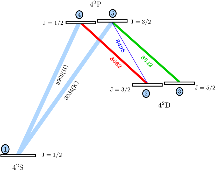
Figure 1.— Atomic model with energy levels for Caii. The labels indicate the spectroscopic terms. Numbers inside blue filled circles identificate each level. Solid lines connecting levels show the allowed radiative transitions and the numbers at the middle of each segment are their wavelength in Å. The wider the width of each connecting line the larger the spontaneous emission rate $A_{ul}$ of the transition. Atomic data for each spectral line are shown in Table 1.

$\lambda$ (Å )	$u$	${\ell}$	$A_{u{\ell}}$ (s-1)	$w_{J_{\ell}J_{u}}^{(2)}$	$w_{J_{u}J_{\ell}}^{(2)}$
Allowed transitions
3934 (K)	5	1	$1.4\times 10^{8}$	$0$	$\sqrt{2}/2$
3969 (H)	4	1	$1.4\times 10^{8}$	$0$	$0$
8498	5	2	$1.11\times 10^{6}$	$-2\sqrt{2}/5$	$-2\sqrt{2}/5$
8542	5	3	$9.6\times 10^{6}$	$\sqrt{7}/5$	$\sqrt{2}/10$
8662	4	2	$1.06\times 10^{7}$	$\sqrt{2}/2$	$0$

Table 1Short list of Ca ii atomic data parameters. From left to right: the central wavelength, the upper and the lower level of each transition, the radiative rates from NIST atomic spectra database (http://www.nist.gov/physlab/data/asd.cfm) and the atomic polarizability coefficients introduced by Landi Degl’Innocenti (1984).

Since the radiation field is axially symmetric, just two radiation field tensor elements ($J^{0}_{0}$ and $J^{2}_{0}$) are necessary to describe the symmetry properties of the spectral line radiation. Let $I(\nu,\mu)$ and $Q(\nu,\mu)$ be the Stokes parameters expressed in the observer’s frame at a given height $z$, where $\nu$ is the frequency, $\mu=\cos\theta$ and $\theta$ is the angle that the ray forms with the vertical direction. Then, the corresponding values seen by a comoving frame with vertical velocity $v_{z}$ with respect to the observer’s frame are $I^{\prime}(\nu^{\prime},\mu)=I(\nu,\mu)$ and $Q^{\prime}(\nu^{\prime},\mu)=Q(\nu,\mu)$, where $\nu^{\prime}=\nu(1-v_{z}\mu/c)$ and $\nu=\nu^{\prime}(1+v_{z}\mu/c)$ (to first order in $v_{z}/c$). Therefore, the mean intensity at the considered height, can be expressed from one or another reference frame as:

$$\bar{J}^{0}_{0} =\frac{1}{2}\int d\nu\int_{-1}^{1}d\mu\phi^{\prime}_{\ell u}(\nu,\mu)I(\nu,\mu)$$

$$=\frac{1}{2}\int d\nu^{\prime}\int_{-1}^{1}d\mu\phi_{\ell u}(\nu^{\prime})I(\nu^{\prime}(1+v_{z}\mu/c),\mu),$$ (2)

where $\phi_{\ell u}(\nu)$ is the absorption profile (e.g., for a Gaussian profile, we would have $\phi_{\ell u}(\nu)=\pi^{-1/2}{\Delta\nu_{D}}^{-1}\exp(-(\nu-\nu_{0})^{2}/{\Delta\nu_{D}}^{2})$, with $\nu_{0}$ the central line frequency and $\Delta\nu_{D}$ the Doppler width) and $\phi^{\prime}_{\ell u}(\nu,\mu)=\phi_{\ell u}(\nu(1-v_{z}\mu/c))$, with $v_{z}>0$ for upflowing material. Analogously, the anisotropy in the observer’s frame:

$$\bar{J}^{2}_{0} = \frac{1}{4\sqrt{2}}\int d\nu\int_{-1}^{1}d\mu\phi_{\ell u}^{\prime}(\mu,\nu)$$ (3)

$$\times [(3\mu^{2}-1)I(\nu,\mu)+3(1-\mu^{2})Q(\nu,\mu)],$$

The important quantity that controls the ability of an anisotropic radiation field to generate atomic polarization is the line anisotropy factor for each transition, which can be calculated as:

$${\sc}w_{\mathrm{line}}={\sqrt{2}}\frac{\bar{J}^{2}_{0}}{\bar{J}^{0}_{0}}.$$ (4)

Its range goes from $\sc w_{\mathrm{line}}=-0.5$ (for a radiation field coming entirely from the horizontal plane) to $\sc w_{\mathrm{line}}=1$ (for a collimated vertical beam).

2.2. The radiative transfer equations (RTE)

Due to symmetry, in a non-magnetized plane-parallel medium with a vertical velocity field, light can only be linearly polarized parallel or perpendicularly to the stellar limb. Therefore, chosing the reference direction for positive $Q$ parallel to the limb, the only non-vanishing Stokes parameters are $I$ and $Q$, and they satisfy the following radiative transfer equations:

$$\frac{\rm d}{{\rm d}s}I =\epsilon_{I}-\eta_{I}I-\eta_{Q}Q,$$ (5a)

$$\frac{\rm d}{{\rm d}s}Q =\epsilon_{Q}-\eta_{Q}I-\eta_{I}Q,$$ (5b)

where $s$ is the distance along the ray. The absorption and emission coefficients are (MSTB2010):

$$\epsilon_{I} =\,\epsilon_{I}^{\rm cont}+\epsilon_{I}^{\rm line}$$

$$=\,{\eta_{I}}^{\rm cont}B_{\nu}+\epsilon_{0}\left[\rho^{0}_{0}(u)+w_{J_{u}J_{\ell}}^{(2)}\frac{1}{2\sqrt{2}}(3\mu^{2}-1)\rho^{2}_{0}(u)\right],$$ (6a)

$$\eta_{I} =\,\eta_{I}^{\rm cont}+\eta_{I}^{\rm line}$$

$$=\,{\eta_{I}}^{\rm cont}+\eta_{0}\left[\rho^{0}_{0}(\ell)+w_{J_{\ell}J_{u}}^{(2)}\frac{1}{2\sqrt{2}}(3\mu^{2}-1)\rho^{2}_{0}(\ell)\right],$$ (6b)

$$\epsilon_{Q}\,=\,\epsilon^{\rm line}_{Q}\,=\,\epsilon_{0}w_{J_{u}J_{\ell}}^{(2)}\frac{3}{2\sqrt{2}}(1-\mu^{2})\rho^{2}_{0}(u),$$ (7a)

$$\eta_{Q}\,=\,\eta^{\rm line}_{Q}\,=\,\eta_{0}w_{J_{\ell}J_{u}}^{(2)}\frac{3}{2\sqrt{2}}(1-\mu^{2})\rho^{2}_{0}(\ell),$$ (7b)

where ${\eta_{I}}^{\rm cont}$ and ${\epsilon_{I}}^{\rm cont}$ are the continuum absortion and emission coefficients for intensity, respectively. Likewise, $\eta_{I}^{\mathrm{line}}$ and $\eta_{Q}^{\mathrm{line}}$ are the line absorption coefficients for Stokes $I$ and $Q$, respectively, while $\epsilon_{I}^{\mathrm{line}}$ and $\epsilon_{Q}^{\mathrm{line}}$ are the line emission coefficients for Stokes $I$ and $Q$, respectively. The coefficients $w_{J_{\ell}J_{u}}^{(2)}$ and $w_{J_{u}J_{\ell}}^{(2)}$ depend only on the transition and are detailed in Table (1).The subscripts $u$ and $\ell$ refer to the upper and lower level of the transition considered, respectively, and $B_{\nu}$ is the Planck function at the central frequency $\nu_{0}$ of the transition. Note also that:

$$\epsilon_{0}=\frac{h\nu}{4\pi}A_{u{\ell}}{\phi^{\prime}_{\ell u}(\mu,\nu)}{\cal N}\sqrt{2J_{u}+1},$$ (8a)

$$\eta_{0}=\frac{h\nu}{4\pi}B_{{\ell}u}{\phi^{\prime}_{\ell u}(\mu,\nu)}{\cal N}\sqrt{2J_{\ell}+1},$$ (8b)

where $\cal N$ is the total number of atoms per unit volume.

With the total absortion coefficient for the intensity, the line of sight (los) optical depth for each frequency is calculated by the following integral along the ray:

$$\tau^{\rm los}_{\nu}=-\int\eta_{I}(\mu^{\rm los},\nu)\frac{dz}{\mu^{\rm los}}$$ (9)

2.3. Numerical method

The solution to the non-LTE problem of the second kind considered here (the self-consistent solution of the statistical equilibrium equations for the density matrix elements together with the radiative transfer equations for the Stokes parameters) is carried out by generalizing the computer program developed by Manso Sainz & Trujillo Bueno (2003), to allow for radial macroscopic velocity fields. For integrating the RTE, a parabolic short-characteristics scheme (Kunasz & Auer, 1988) is used. At each iterative step, the radiative transfer equation is solved, and $\bar{J}^{0}_{0}$ and $\bar{J}^{2}_{0}$ are computed and used to solve the SEE following the accelarated Lambda iteration method outlined in the Appendix of MSTB2010. Once the solution for the multipolar components of the density matrix is consistently reached, the emergent Stokes parameters are calculated for the desired line of sight, which in all the figures of this paper is $\mu=0.1$. This final step is done increasing the frequency grid resolution to a large value in order to correctly sample the small features and peaks of the emergent profiles.

Some technical considerations have to be kept in mind for the treatment of velocity fields. Due to the presence of Doppler shifts, the wavelength axis used to compute $\bar{J}^{0}_{0}$ and $\bar{J}^{2}_{0}$ must include the required extension and resolution, because the spectral line radiation may be now shifted and asymmetric. In our strategy for the wavelength grid, the resolution is larger in the core than in the wings, keeping the same wavelength grid for all heights.

The cutoff wavelength for the core (where resolution is appreciably higher) is dictated by the maximum expected Doppler shift. Thus, the core bandwidth is estimated allowing for a range of $2V_{\rm{max}}$ around the zero velocity central wavelength of the lines, with $V_{\rm{max}}$ the maximum velocity found in the atmosphere (in Doppler units). Apart from that, a minimum typical resolution for the core is set to 2 points per Doppler width ($\Delta\nu_{D}$). Then, the height with the smallest Doppler width determines the core resolution, and the height with the maximum macro-velocity states its bandwidth.

Furthermore, as frequencies and angles are inextricably entangled (through terms $\nu-v_{z}\mu\nu/c$ appearing in the absortion/emission profiles due to the Doppler effect, like in Eq. (2.1)), the maximum angular increment ($\Delta\mu_{\rm{max}}$) is restricted by the maximum frequency increment ($\Delta x_{\rm{max}}\thickapprox 1/2$, in Doppler units). Thus, it must occur that $\Delta\mu_{\rm{max}}\cdot V_{\rm{max}}\leq 1/2$. In the worst case, the maximum allowed angular increment will be smaller (more angular resolution needed) when the maximum vertical velocity increases. Besides this consideration, the maximum angular increment could be even more demanding because of the high sensitivity of the polarization profiles to the angular discretization.

Finally, the depth grid must be fine enough, in such a way that the maximum difference in velocity between consecutive points is not too large, the typical difference being equal to half the Doppler width ($|V(z_{i})-V(z_{i-1})|\leq 1/2$). If the difference is larger, the absortion/emission profiles would change abruptly with height, producing imprecisions in the optical depth increments (Mihalas, 1978).

3. Effect of a velocity gradient on the radiation field anisotropy and the mean intensity

As we shall see, the presence of a vertical velocity gradient in an atmosphere enhances the anisotropy of the radiation field and, hence, of the scattering line polarization patterns. The fundamental process underlying this mechanism can be simply understood with the following basic examples.

3.1. Anisotropy seen by a moving scatterer.

Consider an absorption spectral line with a Gaussian profile emerging from a static atmosphere with a linear limb darkening law,

$$I(\nu,\mu)=I^{(0)}(1-u+u\mu)[1-a\exp(-(\frac{\nu-\nu_{0}}{w})^{2})],$$ (10)

where $I^{(0)}$ is the continuum intensity at disk center, $u$ is the limb darkening coefficient, $a<1$ measures the intensity depression of the line, and $w$ its width. In this approximation we assume that all the parameters are constant. Now imagine that, at the top of the atmosphere, there is a thin cloud scattering the incident light given by Eq. (10) and moving radially at velocity $v_{z}$ with respect to the bottom layers of the atmosphere, supposed static. We will assume that the absorption profile is Gaussian (dominated by Doppler broadening), with width $\Delta\nu_{D}$. When $\Delta\nu_{D}\ll w$, the incident spectral line radiation is much broader than the absorption profile (in fact, for $\alpha=\Delta\nu_{D}/w=0$ the absorption profile is formally a Dirac-$\delta$ function). Then, from Equations (2.1)-(3) we can derive explicit expressions for the mean intensity and anisotropy of the radiation field as a function of the scatterer velocity (see Appendix A): $\bar{J}^{0}_{0}={\cal I}_{0}(\alpha;\xi)/2$, $\bar{J}^{2}_{0}={\cal I}_{2}(\alpha;\xi)/4\sqrt{2}$, where the ${\cal I}_{0,2}$ functions are defined by Equations (A)-(A). The behaviour of $\bar{J}^{0}_{0}$ and $\bar{J}^{2}_{0}$ with the adimensional velocity $\xi=v_{z}\nu_{0}/(cw)$ (Figure 2), is most clearly illustrated in their asymptotic limits at low velocities:

$$\bar{J}^{0}_{0} =\frac{1}{4}(1-\frac{a}{\sqrt{1+\alpha^{2}}})(2-u)$$

$$+ \frac{a(4-u)}{12(1+\alpha^{2})^{3/2}}\xi^{2}+{\rm O}(\xi^{3}),$$ (11)

$$\sqrt{2}\frac{\bar{J}^{2}_{0}}{\bar{J}^{0}_{0}} =\frac{u}{4(2-u)}$$

$$+ \frac{a(64-56u+7u^{2})}{120(2-u)^{2}(1+\alpha^{2})(\sqrt{1+\alpha^{2}}-a)}\xi^{2}+{\rm O}(\xi^{3}).$$ (12)

Equation (11) shows that, for an absorption line ($a>0$), $\bar{J}^{0}_{0}$ is always increasing with the velocity since the coefficient of $\xi^{2}$ is positive, and this, regardless of the sign of $v_{z}$ (i.e., regardless of whether the scatterers move upwards or downwards); if the line is in emission ($a<0$), $\bar{J}^{0}_{0}$ monotonically decreases. These are the Doppler brightening and Doppler dimming effects (e.g., Landi Degl’Innocenti & Landolfi, 2004). An analogous analysis applies to $\bar{J}^{2}_{0}$ (Eq. 12). Note that, in the absence of limb darkening ($u=0$), the anisotropy vanishes in a static atmosphere, while the mere presence of a relative velocity between the scatterers and the underlying static atmosphere induces anisotropy in the radiation field —hence, a polarization signal. A real atmosphere could then be understood as a superposition of scatterers that modify the anisotropy depending on the local velocity gradient and the illumination received from lower shells. An interesting discussion on the effect of velocities with directions other than radial can be found in Landi Degl’Innocenti & Landolfi (2004; Section 12.4).

Figure 2.— $\bar{J}^{0}_{0}/I^{(0)}$ (upper panel) and $\sqrt{2}\bar{J}^{2}_{0}/\bar{J}^{0}_{0}$ (lower panel) as a function of the adimensional velocity $\xi$ calculated using an incident line profile as in Eq. (10) with $u=0.3$ and $a=0.4$ or 0.8 (see labels). Dotted lines have been computed for the case of an infinitely sharp absorption profile ($\alpha=0$). Solid lines refer to the case $\alpha=0.9$ (non saturated line). The case with no limb darkening ($u=0$) and $a=0.4$ has been plotted for comparison (dashed lines).

Figure 3.— Adimensional velocity fields considered in this section. They are parameterized by the limiting value at small optical depths (labels) and by the location in optical depth of the largest velocity gradient region (vertical lines marking $\tau_{0}$). Solid lines: $\tau_{0}=1$. Dotted lines: $\tau_{0}=100$.

Figure 4.— $\bar{J}^{0}_{0}$ (upper panel) and $\sqrt{2}\bar{J}^{2}_{0}/\bar{J}^{0}_{0}$ (lower panel) as a function of the integrated static line opacity ($\tau_{l}$) in an expanding atmosphere with $S=S^{(0)}(1+\beta\tau_{l})$ and different velocity stratifications $\xi=\xi_{0}/(1+\tau_{l}/\tau_{0})$ (see Fig. 3). The parameters used in this plot are $\beta=3/2$ and $\kappa_{c}/\kappa_{l}=10^{-4}$. The labels indicate the value of $\xi_{0}$. Solid lines correspond to $\tau_{0}=1$ while dotted lines refer to $\tau_{0}=100$.

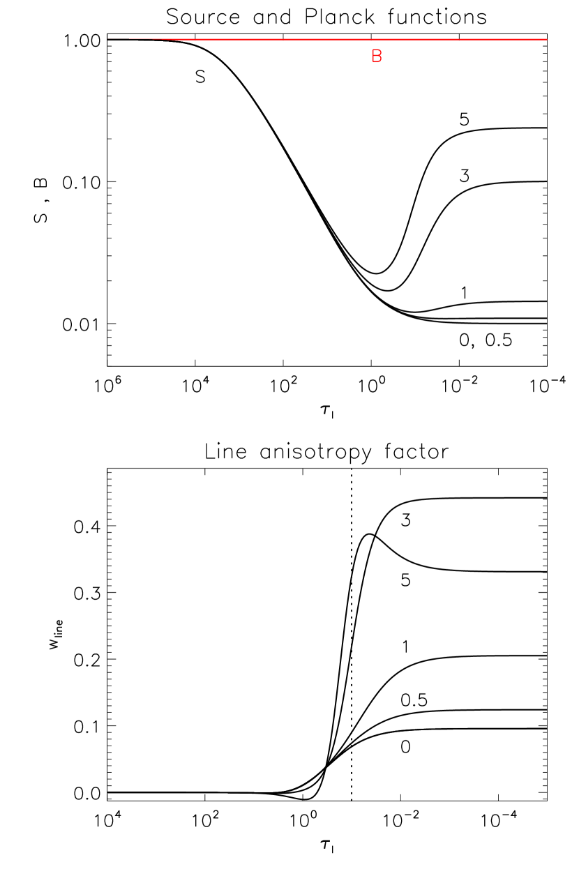
Figure 5.— Same as Fig. 4 for an isothermal moving atmosphere with a two-level atom model using the velocity fields of Fig. 3. We assume a very strong line ($r_{c}=0$) and $\epsilon=10^{-4}$. Upper panel: the Doppler brightening effect increases the surface source function value. In a two-level model atom in a static atmosphere (label 0) this value follows the well known expression $S(0)=\sqrt{\epsilon}B$. The vertical axis is in units of the Planck function. Lower panel: we show the amplification of the radiation field anisotropy when the velocity gradient increases. The vertical line marks the location of the largest velocity gradient ($\tau_{l}=\tau_{0}=0.1$). The curve labeled with “5” shows the saturation of the anisotropy and the bump produced by the strong velocity gradient taking place at optically thin regions.

Clearly, all the above discussion depends on the Doppler shift induced by the velocity $v_{z}$ normalized to the width of the spectral line, i.e., on $\xi$. A large velocity gradient on a broad line has the same effect as that of a smaller velocity gradient on a narrow line. This is important to be kept in mind since the response of different spectral lines to the same velocity gradient will be different, what can help us to decipher the velocity stratification. Even different spectral lines belonging to the same atomic species may have very different widths, as for example, the Ca ii IR triplet and the UV doublet studied in the next section.

3.2. Calculations in a Milne-Eddington model.

The discussion above explains the basic mechanism by means of which a velocity gradient enhances the anisotropy of the radiation field. Now we can get further insight on the structure of the radiation field within an atmosphere with velocity gradients from just the formal solution of the RT equation for the intensity (e.g., Mihalas 1978). As before, we neglect effects due to polarization and $J^{0}_{0}$ and $J^{2}_{0}$ are calculated from Stokes $I$ alone. We consider a semi-infinite, plane-parallel atmosphere with a source function $S=S_{0}(1+\beta\tau_{l})$, where $\tau_{l}$ is the integrated line optical depth in the static limit (hence, the element of optical depth $d\tau_{\nu}=(r+\phi[\nu(1-v_{z}(\tau_{l})\mu/c)])d\tau_{l}$, where $r=\kappa_{c}/\kappa_{l}$ is the ratio of continuum to line opacity). We begin by considering a vertical velocity field $v_{z}(\tau_{l})=v_{0}/[1+(\tau_{l}/\tau_{0})]$ (positive outward the star), shown in Fig. 3. Equivalently, we may express the velocity in adimensional terms by using $\xi=(\nu_{0}/c)v_{z}/\Delta\nu_{D}$ (the width $\Delta\nu_{D}$ of the Gaussian absorption profile is assumed to be constant with depth). The parameter $\tau_{0}$ fixes the position of the maximum velocity gradient. Note that the wavelength dependence of the Doppler effect ($\Delta\lambda_{z}=\lambda_{0}v_{z}/c$) is cancelled in the adimensional problem, where velocities are measured in Doppler units. It is easy to calculate numerically $I_{z}(\nu,\mu)$ at every point in the atmosphere and thus, the mean intensity and anisotropy of the radiation field (Figure 4).

The rise in $\bar{J}^{0}_{0}$ in higher layers with respect to the static case corresponds to the Doppler brightening discussed above. Thanks to the Doppler shifts, the atoms see more and more of the brighter continuum below, which enhances $\bar{J}^{0}_{0}$. When the maximum velocity gradient takes place at optically thick enough layers ($\tau_{0}\gtrsim 1$), $\bar{J^{0}_{0}}$ is also larger than for the static case, but it decreases monotonically with height in the atmosphere ($\tau_{0}=10^{2}$, dotted lines in upper panel of Fig. 4). Note that the important quantity that modulates the increase in $\bar{J^{0}_{0}}$ is not the maximum velocity but the velocity gradient (difference in velocity between optically thick and optically thin parts of the atmosphere). The larger the gradient, the more pronounced the radiative decoupling is between different heights. An extreme example of such radiative decoupling could be found in supernovae explosions, where the vertical velocity gradients are huge.

In our case (vertical motions), the Doppler brightening implies an enhancement of the contribution of vertical radiation to Eq. (3) with respect to the horizontal radiation, with the latter remaining almost equal to the static case (no horizontal motions, no horizontal Doppler brightening). This velocity-induced limb darkening is the origin of the anisotropy enhancement.

However, note that the maximum anisotropy does not rise indefinitely when increasing the maximum velocity. If the velocity gradient in units of the Doppler width is larger than $\sim 3$ (see curves for $\xi_{\rm{max}}=5$ in Fig. 4), the anisotropy at the surface saturates and decreases (even below the curves corresponding to shorter velocity gradients). It is accompanied by a bump around $\tau_{l}=1$ when the maximum velocity gradient is taking place at low density layers ($\tau_{0}\lesssim 1$). This behavior can be understood using Eq. (3). When $\xi_{\rm{max}}\lesssim 3$, an increment in $\xi_{\rm{max}}$ entails a rise in $\bar{J}^{0}_{0}$, $\bar{J}^{2}_{0}$ and $\bar{J}^{2}_{0}/\bar{J}^{0}_{0}$ ($w_{\rm{line}}$) in the upper atmosphere, what means that the velocity gradients enhance the imbalance between vertical and horizontal radiation. However, if $\xi_{\rm{max}}$ is above that threshold, $\bar{J}^{0}_{0}$ and $\bar{J}^{2}_{0}$ rise, but the ratio $\bar{J}^{2}_{0}/\bar{J}^{0}_{0}$ saturates and diminishes. The reason is that a large velocity gradient makes the absorption profiles associated to almost horizontal outgoing rays ($0<\mu<1/\sqrt{3}$) shifted so much that they also capture the background continuum radiation. Their contributions are negative to the angular integral of $\bar{J}^{2}_{0}$ but positive for $\bar{J}^{0}_{0}$.

Separating the contributions of rays with angles in the range $1/\sqrt{3}<|\mu|<1$ (that we refer to with the label $+$) and angles in the range $0<|\mu|<1/\sqrt{3}$ (that we refer to with the label $-$), the line anisotropy can be written as $w_{\rm{line}}=w^{+}_{\rm{line}}+w^{-}_{\rm{line}}=\bar{J}^{2+}_{0}/\bar{J}^{0}_{0}-|\bar{J}^{2-}_{0}|/\bar{J}^{0}_{0}$. Here, $\bar{J}^{0}_{0}$ and $\bar{J}^{2+}_{0}$ grow always with $\xi_{\rm{max}}$, but $|\bar{J}^{2-}_{0}|$ only grows appreciably when $\xi_{\rm{max}}\gtrsim 3$. Therefore, although $w_{\rm{line}}$ increases for all velocity gradients, its enhancement is smaller for large velocity gradients than for smaller ones. This effect occurs as well when motions take place deeper ($\tau_{0}\gtrsim 1$) but it is less important and the anisotropy bump and saturation are reduced.

For the considered velocity fields (with a negligible gradient in the upper atmosphere), $\bar{J}^{0}_{0}$ and $\bar{J}^{2}_{0}$ reach an asymptotic value in optically thin regions. We have verified that this effect does not occur if the velocity gradient is not zero in those layers. In any case, the presence of a large anisotropy in optically thin heights barely affects the emergent linear polarization profiles.

3.3. Two-level model atom in dynamic atmospheres.

Before going to a more realistic case, a final illustrative example is considered. In this case, we assume the same parameterization of the velocities than in the previous example, but now we solve the complete iterative RT problem with a two-level atom model and a specific temperature stratification. Consequently, the source function and the anisotropy are consistently obtained in a moving atmosphere. The intensity source function is $S_{I}=r_{\nu\mu}S^{\rm{line}}_{I}+(1-r_{\nu\mu})B$ (e.g., Rybicki & Hummer, 1992), with $r_{\nu\mu}=\phi^{\prime}_{\ell u}(\nu,\mu)/(r_{c}+\phi^{\prime}_{\ell u}(\nu,\mu))$ and the expression for the line source function remains formally equal to that of the static case, being $S^{\rm{line}}_{I}=(1-\epsilon)\bar{J}^{0}_{0}+\epsilon B$, where $B$ is the imposed Planck function, $\epsilon$ is the inelastic collisional parameter and $\bar{J}^{0}_{0}$ is calculated with Eq. (2.1).

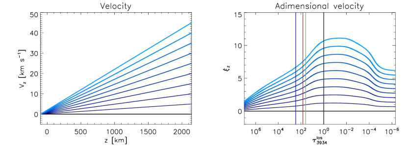
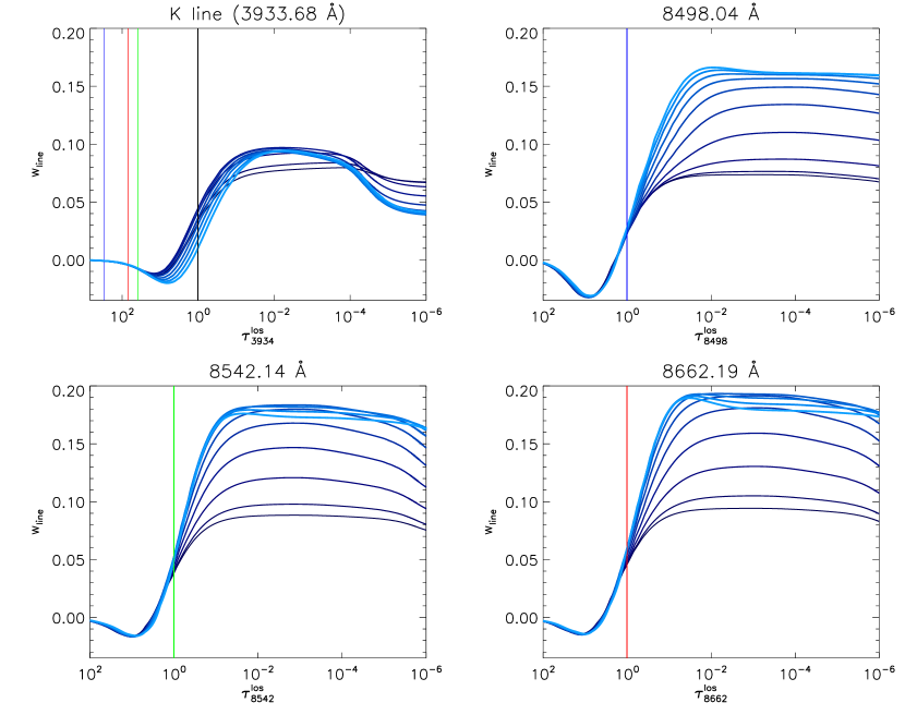
Figure 6.— Amplification of the line anisotropy ($\rm{w_{line}}=\sqrt{2}\bar{J}^{2}_{0}/\bar{J}^{2}_{0}$) due to vertical velocity gradients. Upper left panel: linear velocity fields versus height, with velocity gradients going from $0$ (darker lines) to $20\,\rm{m\cdot s^{-1}\,km^{-1}}$ (light blue lines) in steps of $2.23\,\rm{m\cdot s^{-1}\,km^{-1}}$. Upper right panel: corresponding adimensional velocity fields ($\xi_{z}$) for a FALC temperature stratification and a constant microturbulent velocity of $3.5\,\rm{km\,s^{-1}}$. The horizontal axis is in units of the K-line optical depth along the line of sight (los). The vertical lines mark the position of $\tau^{\rm{los}}_{\nu_{0}}=1$ for the transitions $8498\AA$ (blue), $8542\AA$ (green), $8662\AA$ (red) and the K line (black). Remaining panels: corresponding line anisotropy factors plotted against $\tau^{\rm{los}}_{\nu_{0}}$ for each line.

The qualitative behaviour explained in the previous subsection is maintained in these two-level atom calculations. For small $\epsilon$ values (large NLTE effects), the source function $S_{I}\thickapprox\bar{J}^{0}_{0}$ shows Doppler brightening effects and its surface value depends on the maximum velocity gradient and on the maximum background continuum set by the photospheric conditions (upper panel in Fig. 5). The anisotropy rises proportionally to the velocity gradient until a saturation occurs (lower panel in Fig. 5). A similar behavior is found when the maximum velocity gradient occurs higher in the atmosphere (see Fig. 10 in Appendix C).

In a static atmosphere, the radiation field anisotropy is dominated by the presence of gradients in the intensity source function (Trujillo Bueno 2001; Landi Degl’Innocenti & Landolfi 2004), which can be modified via the Planck function (equivalently, the temperature). In the dynamical case that we are dealing with, the slope of the source function is also modified due to the existence of velocity gradients thanks to the frequency-decoupling caused by relative motions between absortion profiles (Doppler brightening). In general, both mechanisms act together (velocity-induced and temperature-induced modification of the source function gradient) and the ensuing anisotropy and the emergent linear polarization profiles are modified accordingly.

It is important to note that the adimensional velocity $\xi$ depends both on the velocity and also on the line Doppler width because $\xi(\tau)=\delta\nu/\Delta\nu_{D}=v_{z}/\sqrt{2k_{B}T/m}$, with $k_{B}$ the Boltzmann constant, $T$ the temperature and $m$ the mass of the atom. In the photosphere, where velocities are much lower than in the chomosphere, $\xi$ is expected to be negligible. In the chromosphere, plasma motions are important and the temperature is still comparable to that of the photosphere, inducing $\xi$ to be controlled by the velocity field. However, for layers in the transition region and above, the high temperatures reduce the value of $\xi$. In any case, at these heights, the density is so low that, although $\xi$ (and consequently the anisotropy) could have a highly variable behaviour, the emergent polarization profiles of chromospheric lines will not be sensitive to them.

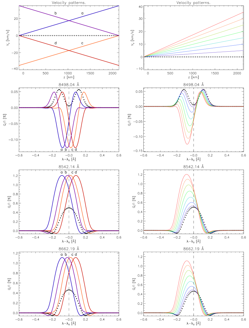
Figure 7.— Left panels: calculation at $\mu=0.1$ of the emergent $Q/I$ polarization signals of the Ca ii IR triplet when four different choices for the vertical velocity gradients are imposed. Positive velocities imply upflowing plasma. Gradient “a”/“b” simulates an atmosphere where the plasma is entirely moving towards the observer increasing/decreasing linearly the velocity along the outgoing z axis. Gradients “c” and “d” are the same for plasma moving away from the observer. The black dotted line is the solution for the static reference case. Each curve is computed on the converged solution of the multilevel NLTE problem described in Sec. 2. Right panels: same calculations than in the left-hand panels, but with different velocity gradient values varying from $0$ to $16.3\,\rm{m\,s^{-1}\,km^{-1}}$ in steps of $2.3\,\rm{m\,s^{-1}\,km^{-1}}$ (see top right panel). These results show that the polarization signals are increased and shifted with respect to the static case depending only on the absolute value of the vertical velocity field gradient and independently of the sign of the velocity field.

4. Results for the Ca ii IR Triplet .

Now, we study the effect of the velocity field on a multilevel atomic system in a realistic atmospheric model, within the more general framework described in Sec. 2. We consider the formation of the scattering polarization pattern of the Ca ii infrared triplet in a semi-empirical model atmosphere (FAL-C model of Fontenla, Avrett, and Loeser 1993) in the presence of vertical velocity fields ($\mathbf{v}=v_{z}(z)\mathbf{k}$, with $\mathbf{k}$ the unit vector along the vertical pointing upwards). We will assume a constant microturbulent velocity field of 3.5 km s^-1, a representative value for the region of formation which gives a realistic broadening of the triplet profiles.

4.1. Behaviour of the anisotropy in the Ca ii IR triplet

For simplicity, we set linear velocity fields (constant velocity gradient along z) between $z=-100$ and 2150  km (see Fig. 6). Consequently, the adimensional velocity field $\xi_{z}$ has a non-monotonic behavior due to its dependence on the temperature (upper right panel in Fig. 6). In the chromosphere, where the Ca ii triplet lines form, $\xi_{z}$ is dominated by the macroscopic motions. Here, the velocity gradients produce variations in the anisotropy of the triplet lines that agree with the behaviour outlined in the previous sections. Namely, an amplification and a subsequent saturation of the anisotropy factor due to the significant velocity gradient at those heights (see the lower panels and middle right panel in Fig. 6). Above the chromosphere, on the contrary, the temperature dominates ($\xi_{z}$ stabilizes and diminishes) and the anisotropy slightly decreases with height.

If the (adimensional) velocity gradient is negligible where the line forms (around $\tau^{\mathrm{los}}_{\nu_{0}}\thicksim 1$), the anisotropy remains unaffected. Otherwise, if a spectral line forms at very hot layers, where the absortion profiles are wider and their sensitivity to the velocity gradients is lower, the Doppler brightening will not be so efficient amplifying the anisotropy. This is the case of the anisotropy of the Ca ii K line (middle left panel in Fig. 6). Compare how the slope of $\xi_{z}$ is smaller where the Ca ii K line forms (black line on Fig. 6) than where the triplet lines do. Consequently, the enhancement of the line anisotropy through the presence of velocity gradients in this line is reduced.

All our calculations demonstrate that the anisotropy in the Ca ii IR triplet can be amplified through chromospheric vertical velocity gradients. This results suggest that the same occurs with the ensuing linear polarization profiles.

4.2. The impact on the polarization of the emergent radiation.

For investigating the effect of vertical velocity fields on the emergent fractional polarization profiles we perform the following numerical experiments. First, we impose velocity gradients with the same absolute value but opposite signs (top left panel of Fig. 7). The resulting emergent $Q/I$ profiles (remaining left panels of Fig. 7) are magnified by a significant factor ($>2$ for all the transitions) with respect to the static case (black dotted line). The linear polarization profiles have the same amplitude, independently of the sign of the velocity gradient. Another remarkable feature is the asymmetry of the profiles, having a higher blue wing in those cases in which the velocity gradient is positive and a higher red wing when the velocity gradient is negative, independently of the velocity sign. Note also that the $Q/I$ profile is shifted in frequency due to the relative velocity between the plasma and the observer.

As a second experiment, we consider different velocity fields with increasing gradients (right upper panel in Fig. 7). In the ensuing $Q/I$ profiles we see that the larger the velocity gradient, the larger the frequency shift of the emergent profiles and the larger the amplitude. In all transitions, one of the lateral lobes of the signal remains almost constant. Thus, what really changes is the central part of the profiles, being a “valley” in the $\lambda 8498$ line and a “peak” in the other two transitions. To quantify these variations, we define $(Q/I)_{\mathrm{pp}}$ (peak-to-peak amplitude of $Q/I$) as the difference between the lowest and the highest value of the emergent $Q/I$ signal, which is also a measure of its contrast. Note that, as expected from the first experiment, $(Q/I)_{\mathrm{pp}}$ depends only on the absolute value of the gradient. Figure 8 summarizes these results.

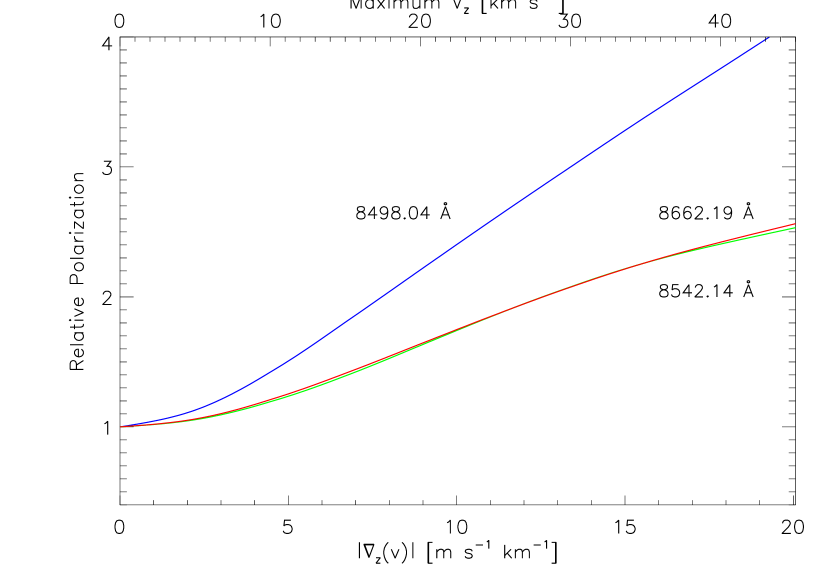
Figure 8.— $(Q/I)_{\mathrm{pp}}$ normalized to the static case solution versus the velocity gradient (bottom axis) and the maximum absolute velocity (top axis) for linear velocity fields appearing in Fig. 7. The results are invariant under velocity sign changes. The transition $\lambda 8498$ is more sensitive to velocity variations due to its thinner absortion profile.

The sensitivity of the linear polarization to the velocity gradient can be measured approximately as commented in Sec. 3.1, using a parameter $\alpha=\Delta\nu_{D}/w$ that accounts for the difference in width of the absorption profile with respect to the emergent intensity profile. If $\alpha\thicksim 1$, small adimensional velocities will produce large changes in shape; if $\alpha\ll 1$, much larger $\xi_{z}$ values are needed for the same effect. In the case of the IR triplet lines, $\alpha\thicksim 0.355$ in the formation region of $\lambda 8498$ and around $0.29$ and $0.285$ in the formation region of $\lambda 8542$ and $\lambda 8662$ (having wider profiles), respectively. Then, the former is more sensitive to velocity variations in its formation region (Fig. 8). Finally, the K line has $\alpha\,(\tau^{\rm{los}}_{\nu_{0}}=1)\thicksim 0.015$, a low value due to its wider spectral wings.

The enhancement of the polarization signals are a consequence of the increase in the anisotropy. Therefore, since this increase is produced by the presence of velocity fields, the polarization signals of the Ca ii IR triplet are sensitive also to the dynamic state of the chromosphere.

4.3. Variations on the atomic alignment due to velocity gradients.

In order to get physical insight on the formation of the emergent polarization profiles, we use an analytical approximation. Following Trujillo Bueno (2003), the emergent fractional linear polarization for a strong line at the central wavelength can be approximated with:

$$\frac{Q}{I}\thickapprox\frac{3}{2\sqrt{2}}(1-\mu^{2})\left[{\sc}w^{(2)}_{J_{u}J_{\ell}}\cdot\sigma^{2}_{0}(J_{u})-{\sc}w^{(2)}_{J_{\ell}J_{u}}\cdot\sigma^{2}_{0}(J_{\ell})\right].$$ (13)

The symbols ${\sc}w^{(2)}_{JJ^{\prime}}$ are numerical coefficients already introduced in Sec. 2. The quantities $\sigma^{2}_{0}(J_{u})$ and $\sigma^{2}_{0}(J_{\ell})$ are the fractional alignment coefficients ($\sigma^{2}_{0}=\rho^{2}_{0}/\rho^{0}_{0}$) evaluated at $\tau^{\rm{los}}_{\nu}=1$ for the upper and lower level of the transition, respectively. This is the generalization of the Eddington-Barbier (EB) aproximation to the scattering polarization and establishes that changes in linear polarization (for a static case) are induced by changes in the atomic aligment of the energy levels.

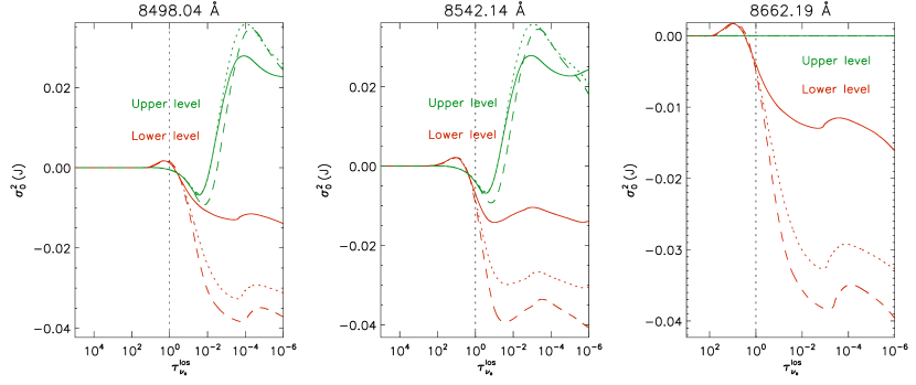
Figure 9.— Behaviour of the fractional alignments $\sigma^{2}_{0}(J_{u})$ (green) and $\sigma^{2}_{0}(J_{l})$ (red) of each Ca ii IR triplet transition for three of the velocity fields shown in Fig. 7. The solid lines correspond to the reference static case. The dotted lines correspond to the case with maximum velocity $15\,\rm{km\,s^{-1}}$. The dashed lines are associated with the case with maximum velocity $30\,\rm{km\,s^{-1}}$. The horizontal axis is the line center optical depth for each value of the velocity gradient. The vertical dotted line marks the height where $\tau^{\rm{los}}_{\nu_{0}}=1.$

Our calculations show that vertical velocity fields with moderate gradients ($\lesssim 10\,\rm{m\,s^{-1}km^{-1}}$ in a linear velocity field, as the ones shown in the figures) do indeed produce variations in the fractional alignment, which are small for $|\sigma^{2}_{0}(J_{u})|$ and significant for $|\sigma^{2}_{0}(J_{\ell})|$ (see Fig. 9). The lower level alignment is the main driver of the changes produced in the $Q/I$ signals. This is strictly true for the $\lambda 8662$ line, whose upper level with $J=1/2$ cannot be aligned (zero field dichroism polarization). In the other transitions, a certain influence of the upper level alignment becomes important only for large gradients. The reason is that the K transition is so strong in comparison with the IR triplet that it is dictating the common upper level 5 alignment (Fig. 1). In fact, $\sigma^{2}_{0}(J_{5})$ is driven by the K line anisotropy which, at cromospheric heights, is almost unaffected for the considered velocity gradients, as we discussed in Sec. 4.1 (Fig. 6). Thus, the strong H and K lines feed population to the upper levels and the K line controls the alignment of the ${}^{2}P_{3/2}$ level (see Fig. 1), while the polarization signals of the IR triplet change with velocity fields affecting $\sigma^{2}_{0}(J_{\ell})$ (through the anisotropy enhancement).

To illustrate the well-known link between the alignment and the anisotropy we can follow the next reasoning. For the Ca ii model atom that we deal with in this work, it is posible to derive a simple analytic expression that relates the anisotropy and the alignments for the $\lambda 8542$ transition. Making use of Eqs. (B4) and (B5) and neglecting second order terms and collisions, we find that:

$${2}\sigma^{2}_{0}(J_{5})-{\sqrt{7}}\sigma^{2}_{0}(J_{3})\simeq{\sc w}_{line}(3\rightarrow 5).$$ (14)

As before, we can roughly assume that $\sigma^{2}_{0}(J_{5})\thicksim\rm{constant}$ at the chromosphere because it is controled by the K line. Then, Eq. (14) suggests that, if the radiation anisotropy increases at that heights, an amplification of $|\sigma^{2}_{0}(J_{3})|$ occurs (note that $\sigma^{2}_{0}(J_{3})$ is negative for these lines). A more aligned atomic population produce a more intense scattering polarization signal.

5. Conclusions

When vertical velocity gradients exist, the polarization profiles are always shifted in wavelength, asymmetrized and enhanced in amplitude with respect to the constant velocity case. The reason is that increments in the absolute value of the velocity gradient increase the source function (Doppler brightening) and enhance the anisotropy of the radiation field (Secs. 3 and 4), that in turn modify the fractional alignment (Sec. 4.3) and amplify the scattering polarization profiles (Sec. 4.2).

For this very reason, all calculations assuming static models in the formation region might underestimate the scattering polarization amplitudes and not capture the right shape of the profiles. In particular, it must be taken into account that the Ca ii IR triplet lines form under non-LTE conditions in chromospheric regions, where velocity gradient may be significantly large due to the upward propagation of waves in a vertically stratified atmosphere (e.g., Carlsson & Stein 1997). Probably, in photospheric and transition region lines the effect of velocities on polarization can be safely neglected (they will be predominantly amplified by temperature gradients as discussed in Sec. 3.3), but not necessarily in the chromosphere. In our study we see that the $\lambda 8498$ line is more sensitive to macroscopic motions in the low-chromosphere, while the $\lambda 8542$ and $\lambda 8662$ lines are especially amplified when strong velocity gradients are found at heights around $1.5\,\rm{Mm}$ and higher in our model.

At the light of these results, it is obvious that the effect of the velocity might be of relevance for measuring chromospheric magnetic fields. In particular, the described mechanism might turn out to be important for the correct interpretation of polarization signals in the Sun with the Hanle effect. Given that weak chromospheric magnetic fields are inferred with the Hanle effect using the difference between the observed linear polarization signal and the signal that would be produced in the absence of a magnetic field, it is crucial to correctly compute the reference no-magnetic signal. In the Ca ii IR triplet, it could be possible to break the degeneracy of the combined effects by taking into account the different sensitivities of the three lines of the triplet to the magnetic field and the thermodynamics. As stated by MSTB2010, the $\lambda 8498$ line is very sensitive to the thermal structure of the atmosphere. Likewise, the response of this line to the velocity gradient is also higher than in the other two. Then, a first step could be to characterize the response of all the lines to combined variations of the temperature, velocity and magnetic field and find observables (i.e., amplitude ratios) that are as insensitive to the temperature and velocity as possible and as sensitive to the magnetic field as possible. We are currently carrying out this study on realistic velocity fields, including shocks and temporal variations.

The polarization amplification mechanism that we have discussed in this paper is not limited to plane-parallel atmospheres, although its effect is surely more important in plane-parallel atmospheres than in three-dimensional ones. The reason is that i) gradients in a three-dimensional atmosphere are weaker given the increased degrees of freedom and ii) non-resolved motions or large variations in velocity direction along the medium mix the contribution of different layers and broaden the profiles, diminishing them in amplitude. In any case, strong three-dimensional velocity gradients might create preferred directions along which the plasma becomes more optically thin through the radiative uncoupling mechanism discussed in this paper.

The amplification of the radiation field anisotropy through vertical velocity gradients is a general and interesting phenomenon that improves our understanding of the stellar atmospheres. With the present investigation we have obtained some feeling about the formation of the Ca ii IR triplet in dynamic situations.

Appendix A Special functions in section 3

Introducing Equation 10 into Equation 2.1

$$\bar{J}^{0}_{0}=\frac{1}{2}\int_{0}^{\infty}d\nu^{\prime}\frac{1}{\sqrt{\pi}\Delta\nu_{D}}\exp\{-(\frac{\nu^{\prime}-\nu_{0}}{\Delta\nu_{D}})^{2}\}\int_{0}^{1}d\mu I^{(0)}(1-u+u\mu)[1-a\exp\{-(\frac{\nu^{\prime}(1+v_{z}\mu/c)-\nu_{0}}{w})^{2}\}].$$ (A1)

Introducing the variables $x=(\nu^{\prime}-\nu_{0})/w$, $\alpha=\Delta\nu_{D}/w$, and $\xi=v_{z}\nu_{0}/(cw)$, then the mean intensity in the comoving frame

$$\frac{\bar{J}^{0}_{0}}{I^{(0)}}=\frac{1}{2}\int_{-\infty}^{\infty}dx\frac{1}{\sqrt{\pi}\alpha}{\rm e}^{-(x/\alpha)^{2}}\int_{0}^{1}d\mu(1-u+u\mu)(1-a\exp^{-(x+\xi\mu)^{2}}).$$ (A2)

In passing from Equation (A1) to Equation (A2), we have extended the integration limit on $x$ to $\infty$. Analogously for the anisotropy in the comoving frame

$$\frac{\bar{J}^{2}_{0}}{I^{(0)}}=\frac{1}{4\sqrt{2}}\int_{-\infty}^{\infty}dx\frac{1}{\sqrt{\pi}\alpha}{\rm e}^{-(x/\alpha)^{2}}\int_{0}^{1}d\mu(3\mu^{2}-1)(1-u+u\mu)(1-a{\rm e}^{-(x+\xi\mu)^{2}}).$$ (A3)

The following integrals are easily evaluated (see Spiegel & Liu, 1998)

$${\cal I}_{0}(\alpha;\xi) \equiv\int_{-\infty}^{\infty}dx\frac{1}{\sqrt{\pi}\alpha}{\rm e}^{-(x/\alpha)^{2}}\int_{0}^{1}(1-u+u\mu)[1-a{\rm e}^{-(x+\xi\mu)^{2}}]d\mu$$

$$=\frac{1}{2}[2-u+a(u-1)\sqrt{\pi}\frac{1}{\xi}{\rm Erf}(\frac{\xi}{\sqrt{1+\alpha^{2}}})+au\sqrt{1+\alpha^{2}}\frac{1}{\xi^{2}}(\exp\{-\frac{\xi^{2}}{1+\alpha^{2}}\}-1)],$$ (A4)

$${\cal I}_{2}(\alpha;\xi) \equiv\int_{-\infty}^{\infty}dx\frac{1}{\sqrt{\pi}\alpha}{\rm e}^{-(x/\alpha)^{2}}\int_{0}^{1}(3\mu^{2}-1)(1-u-u\mu)[1-a{\rm e}^{-(x+\xi\mu)^{2}}]d\mu$$

$$=\frac{1}{4}[u-2a(u-1)\sqrt{\pi}\frac{1}{\xi}{\rm Erf}(\frac{\xi}{\sqrt{1+\alpha^{2}}})+2a\sqrt{1+\alpha^{2}}\frac{1}{\xi^{2}}\left[u+(3-u)\exp\{-\frac{\xi^{2}}{1+\alpha^{2}}\}\right]$$ (A5)

$$+3a(u-1)(1+\alpha^{2})\sqrt{\pi}\frac{1}{\xi^{3}}{\rm Erf}(\frac{\xi}{\sqrt{1+\alpha^{2}}})+6au(1+\alpha^{2})^{3/2}\frac{1}{\xi^{4}}(\exp\{-\frac{\xi^{2}}{1+\alpha^{2}}\}-1)],$$

where we have made use of

$$\int_{-\infty}^{\infty}dx\frac{1}{\sqrt{\pi}\alpha}{\rm e}^{-(x/\alpha)^{2}}[1-a{\rm e}^{-(x+\xi\mu)^{2}}]=1-\frac{a}{\sqrt{1+\alpha^{2}}}\exp\{-\frac{\mu^{2}\xi^{2}}{1+\alpha^{2}}\}.$$ (A6)

From them, the values for $\bar{J}^{0}_{0}$ and the anisotropy $\sqrt{2}\bar{J}^{2}_{0}/\bar{J}^{0}_{0}$ are trivially derived.

In the high velocity limit ($\xi\rightarrow\infty$), ${\cal I}_{0}(\alpha;\xi)=(2-u)/2$, and ${\cal I}_{2}(\alpha;\xi)=u/4$ (regardless of $\alpha$). In the low velocity limit:

$${\cal I}_{0}(\alpha;\xi) =\frac{1}{2}(1-\frac{a}{\sqrt{1+\alpha^{2}}})(2-u)+\frac{a(4-u)}{12(1+\alpha^{2})^{3/2}}\xi^{2}+{\rm O}(\xi^{3}),$$ (A7)

$${\cal I}_{2}(\alpha;\xi) =\frac{u}{4}(1-\frac{a}{\sqrt{1+\alpha^{2}}})+\frac{a(16-u)}{60(1+\alpha^{2})^{3/2}}\xi^{2}+{\rm O}(\xi^{3}).$$ (A8)

Appendix B Statistical equilibrium equations.

The rate equations for the considered problem are as follow. They have been obtained by particularizing to the model-atom of Fig.1 the equations contained in Sects. 7.2 and 7.13 of Landi Degl’Innocenti & Landolfi (2004).

$$\begin{split}\frac{\rm d}{{\rm d}t}\rho^{0}_{0}(1)=&-\biggl{[}\sum_{u=4}^{5}B_{1u}\bar{J}^{0}_{0}(1\rightarrow u)+\sum_{i\neq 1}C_{1i}\biggr{]}\rho^{0}_{0}(1)+A_{41}\rho^{0}_{0}(4)+\sqrt{2}A_{51}\rho^{0}_{0}(5)+\sum_{i\neq 1}C_{i1}\sqrt{\frac{2J_{i}+1}{2}}\rho^{0}_{0}(i),\end{split}$$ (B1)

$$\begin{split}\frac{\rm d}{{\rm d}t}\rho^{0}_{0}(2)=&-\biggl{[}\sum_{u=4}^{5}B_{2u}\bar{J}^{0}_{0}(2\rightarrow u)+\sum_{i\neq 2}C_{2i}\biggr{]}\rho^{0}_{0}(2)-\biggl{(}\frac{1}{\sqrt{2}}B_{24}\bar{J}^{2}_{0}(2\rightarrow 4)-\frac{2\sqrt{2}}{5}B_{25}\bar{J}^{2}_{0}(2\rightarrow 5)\biggr{)}\rho^{2}_{0}(2)\\ &+\frac{1}{\sqrt{2}}A_{42}\rho^{0}_{0}(4)+A_{52}\rho^{0}_{0}(5)+\sum_{i\neq 2}C_{i2}\frac{\sqrt{2J_{i}+1}}{2}\rho^{0}_{0}(i),\end{split}$$ (B2)

$$\begin{split}\frac{\rm d}{{\rm d}t}\rho^{0}_{0}(3)=&-\biggl{[}B_{35}\bar{J}^{0}_{0}(3\rightarrow 5)+\sum_{i\neq 3}C_{3i}\biggr{]}\rho^{0}_{0}(3)-\frac{\sqrt{7}}{5}B_{35}\bar{J}^{2}_{0}(3\rightarrow 5)\rho^{2}_{0}(3)+\sqrt{\frac{2}{3}}A_{53}\rho^{0}_{0}(5)+\sum_{i\neq 3}C_{i3}\sqrt{\frac{2J_{i}+1}{6}}\rho^{0}_{0}(i),\end{split}$$ (B3)

$$\begin{split}\frac{\rm d}{{\rm d}t}\rho^{0}_{0}(4)=&-\biggl{[}\sum_{l=1}^{2}A_{4l}+\sum_{i\neq 4}C_{4i}\biggr{]}\rho^{0}_{0}(4)+\sum_{l=1}^{2}B_{l4}\bar{J}^{0}_{0}(l\rightarrow 4)\sqrt{\frac{2J_{l}+1}{2}}\rho^{0}_{0}(l)\\ &+B_{24}\bar{J}^{2}_{0}(l\rightarrow 4)\rho^{2}_{0}(2)+\sum_{i\neq 4}C_{i4}\sqrt{\frac{2J_{i}+1}{2}}\rho^{0}_{0}(i),\end{split}$$ (B4)

$$\begin{split}\frac{\rm d}{{\rm d}t}\rho^{0}_{0}(5)=&-\biggl{[}\sum_{l=1}^{3}A_{5l}+\sum_{i\neq 5}C_{5i}\biggr{]}\rho^{0}_{0}(5)+\sum_{l=1}^{3}B_{l5}\bar{J}^{0}_{0}(l\rightarrow 5)\frac{\sqrt{2J_{l}+1}}{2}\rho^{0}_{0}(l)\\ &-\frac{2\sqrt{2}}{5}B_{25}\bar{J}^{2}_{0}(2\rightarrow 5)\rho^{2}_{0}(2)+\frac{\sqrt{42}}{10}B_{35}\bar{J}^{2}_{0}(3\rightarrow 5)\rho^{2}_{0}(3)+\sum_{i\neq 5}C_{i5}\frac{\sqrt{2J_{i}+1}}{2}\rho^{0}_{0}(i),\end{split}$$ (B5)

$$\begin{split}\frac{\rm d}{{\rm d}t}\rho^{2}_{0}(2)=&-\biggl{[}\sum_{u=4}^{5}B_{2u}\bar{J}^{0}_{0}(2\rightarrow u)+\sum_{i\neq 2}C_{2i}+D_{2}^{(2)}\biggr{]}\rho^{2}_{0}(2)-\biggl{(}\frac{1}{\sqrt{2}}B_{24}\bar{J}^{2}_{0}(2\rightarrow 4)-\frac{2\sqrt{2}}{5}B_{25}\bar{J}^{2}_{0}(2\rightarrow 5)\biggr{)}\rho^{0}_{0}(2)\\ &+\frac{1}{5}A_{52}\rho^{2}_{0}(5)+\sum_{i=3,5}C_{i2}^{(2)}\frac{\sqrt{2J_{i}+1}}{2}\rho^{2}_{0}(i),\end{split}$$ (B6)

$$\begin{split}\frac{\rm d}{{\rm d}t}\rho^{2}_{0}(3)=&-\biggl{[}B_{35}\bar{J}^{0}_{0}(3\rightarrow 5)+\sum_{i\neq 3}C_{3i}+D_{3}^{(2)}\biggr{]}\rho^{2}_{0}(3)-B_{35}\bar{J}^{2}_{0}(3\rightarrow 5)\frac{\sqrt{7}}{5}\rho^{0}_{0}(3)\\ &+B_{35}\bar{J}^{2}_{0}(3\rightarrow 5)\biggl{[}\sqrt{\frac{5}{7}}\rho^{2}_{0}(3)-\frac{9}{2}\sqrt{\frac{3}{35}}\rho^{4}_{0}(3)\biggr{]}+\frac{2}{5}\sqrt{\frac{7}{3}}A_{53}\rho^{2}_{0}(5)+\sum_{i=2,5}C_{i3}^{(2)}\sqrt{\frac{2J_{i}+1}{6}}\rho^{2}_{0}(i),\end{split}$$ (B7)

$$\begin{split}\frac{\rm d}{{\rm d}t}\rho^{2}_{0}(5)=&-\biggl{[}\sum_{l=1}^{3}A_{5l}+\sum_{i\neq 5}C_{5i}+D_{5}^{(2)}\biggr{]}\rho^{2}_{0}(5)+\frac{1}{5}B_{25}\bar{J}^{0}_{0}(2\rightarrow 5)\rho^{2}_{0}(2)+\frac{\sqrt{21}}{5}B_{35}\bar{J}^{0}_{0}(3\rightarrow 5)\rho^{2}_{0}(3)\\ &+\frac{1}{2}B_{15}\bar{J}^{2}_{0}(1\rightarrow 5)\rho^{0}_{0}(1)-\frac{2\sqrt{2}}{5}B_{25}\bar{J}^{2}_{0}(2\rightarrow 5)\rho^{0}_{0}(2)+\frac{\sqrt{3}}{10}B_{35}\bar{J}^{2}_{0}(3\rightarrow 5)\rho^{0}_{0}(3)\\ &+2\sqrt{\frac{7}{5}}B_{25}\bar{J}^{2}_{0}(2\rightarrow 5)\rho^{2}_{0}(2)-\sqrt{\frac{3}{5}}B_{35}\bar{J}^{2}_{0}(3\rightarrow 5)\rho^{2}_{0}(3)\\ &+\frac{9}{\sqrt{5}}B_{35}\bar{J}^{2}_{0}(3\rightarrow 5)\rho^{4}_{0}(3)+\sum_{i=2,3}C_{i5}^{(2)}\frac{\sqrt{2J_{i}+1}}{2}\rho^{2}_{0}(i),\end{split}$$ (B8)

$$\begin{split}\frac{\rm d}{{\rm d}t}\rho^{4}_{0}(3)=&-\biggl{[}B_{35}\bar{J}^{0}_{0}(3\rightarrow 5)+\sum_{i\neq 3}C_{3i}+D_{3}^{(4)}\biggr{]}\rho^{4}_{0}(3)-B_{35}\bar{J}^{2}_{0}(3\rightarrow 5)\biggl{[}\frac{9}{2}\sqrt{\frac{3}{35}}\rho^{2}_{0}(3)+3\sqrt{\frac{11}{70}}\rho^{4}_{0}(3)\biggr{]},\end{split}$$ (B9)

where $A_{u{\ell}}$ and $B_{{\ell}u}$ are the Einstein emission and absortion coefficients; $C_{{\ell}u}$ and $C_{u{\ell}}$ are the excitation and deexcitation inelastic collisional rates, respectively; $C^{(2)}_{{\ell}u}$ and $C^{(2)}_{u{\ell}}$ are the collisional transfer rates for alignment between polarizable levels (with $J>1/2$); and $D^{(K)}_{i}$ is the depolarization rate of the $K$-th multipole of level ${i}$ due to elastic collisions with neutral hydrogen atoms. The $\rho^{K}_{0}$ elements are referred to a coordinate system with the quantization axis along the solar local vertical direction.

Appendix C Two-level atom calculation in a moving atmosphere.

Figure C1 is similar to Fig. 5, but for velocity fields with $\xi=5$ and maximum gradients occuring at different positions along the atmosphere.

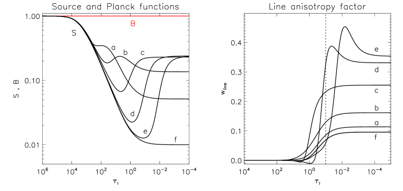
Figure 10.— Calculations in isothermal two-level atom moving atmospheres with $\xi_{max}=5$ . We assume a very strong line ($r_{c}=0$) and $\epsilon=10^{-4}$. The highest velocity gradient occur at $\tau_{l}=\tau_{0}=100,10,1,0.1,0.01$ for a, b, c, d and e, respectively. The case f corresponds to the solution in a static atmosphere. The vertical dotted line marks the position of $\tau_{l}=1$.

References

- Brink & Satchler (1968) Brink, D. M., & Satchler, G. R. 1968, Angular Momentum, 2nd edition, Clarendon Press, Oxford
- Carlsson & Stein (1997) Carlsson, M. & Stein, Robert F., 1997 ApJ, 481,500C
- Fontenla et al. (1993) Fontenla, J. M., Avrett, E. H., & Loeser, R. 1993, ApJ, 406, 319
- Spiegel, M. & Liu, J. (1998) Spiegel,M. & Liu, J.,1998 , Mathematical handbook of formulas and tables, Ed. McGraw-Hill.
- Kunasz & Auer (1988) Kunasz, P., & Auer, L. H. 1988, JQSRT, 39, 67
- Landi Degl’Innocenti (1984) Landi Degl’Innocenti, E., 1984, Solar Physics, 91, 1
- Landi Degl’Innocenti & Landolfi (2004) Landi Degl’Innocenti, E., & Landolfi, M. 2004, Polarization in Spectral Lines (Dordrecht: Kluwer)
- Manso Sainz & Trujillo Bueno (2003) Manso Sainz, R., & Trujillo Bueno, J. 2003, Phys. Rev. Letters, 91, 111102
- Manso Sainz & Trujillo Bueno (2010) Manso Sainz, R. & Trujillo Bueno, J. 2010 ApJ…722.1416M
- Mihalas (1978) Mihalas, D. 1978, Stellar Atmospheres, 2nd Ed. (San Francisco: W. H. Freeman & Comp.)
- Rybicki & Hummer (1992) Rybicki, G. B. & Hummer, D. G., 1992, A&A, 262, 209
- Stenflo (1998) Stenflo, J.O. 1998, A&A , 338, 301S
- Stepan & TrujilloBueno (2010) Štěpán, J. & Trujillo Bueno, J., 2010, Mem. S.A.It. Vol. 81, 810
- Trujillo Bueno (2001) Trujillo Bueno, J. 2001, in Advanced Solar Polarimetry, ed. M. Sigwarth, ASP Conf. Series Vol. 236, 161
- Trujillo Bueno (2010) Trujillo Bueno, J. 2010, in Magnetic Coupling between the Interior and Atmosphere of the Sun, eds. S. S. Hasan & R. J. Rutten, 118T
- Uitenbroek & Socas-Navarro (2004) Uitenbroek, H. & Socas-Navarro, H. 2004, ApJ, 603, 129
- Uitenbroek (2011) Uitenbroek, H. 2011, in Solar Polarization Workshop 6, ASP Conf. Ser. Vol. 437, 439