One-loop renormalization group study of boson-fermion mixtures

A weakly interacting boson-fermion mixture model was investigated using Wisonian renormalization group analysis. This model includes one boson-boson interaction term and one boson-fermion interaction term. The scaling dimensions of the two interaction coupling constants were calculated as $2-D$ at tree level and the Gell-Mann-Low equations were derived at one-loop level. We find that in the Gell-Mann-Low equations the contributions from the fermion loops go to zero as the length scale approaches infinity. After ignoring the fermion loop contributions two fixed points were found in 3 dimensional case. One is the Gaussian fixed point and the other one is Wilson-Fisher fixed point. We find that the boson-fermion interaction decouples at the Wilson-Fisher fixed point. We also observe that under RG transformation the boson-fermion interaction coupling constant runs to negative infinity with a small negative initial value, which indicates a boson-fermion pairing instability. Furthermore, the possibility of emergent supersymmetry in this model was discussed.

1 Introduction

Since the first observation of Bose-Einstein condensation in ⁴He in 1995[1], the field of degenerate quantum gases has become one of the most active areas of physics. Of particular interest is the realization of boson-fermion mixtures of atom gases. They may show very different behavior from pure fermion or pure boson gases. Various theoretical researches have been proposed. For instance, formation of stable strongly correlated boson-fermion pairs[2], instability of the mixture when there is an attraction between bosons and fermions[3, 4], interspecies interactions induced attraction among bosons[5, 6] and emergent supersymmetry (SUSY) from mixtures of cold Bose and Fermi atoms[7, 8]. Recent developments in atomic experiments have made it possible to realize boson-fermion mixed gases in the laboratory. Collapse of the atomic cloud induced by the interspecies attraction in boson-fermion mixtures was observed experimentally[9]. Also, the formation of heteronuclear Feshbach molecules has been observed in a boson-fermion mixture of ⁸⁷Rb and ⁴⁰K atomic vapors in a 3D optical lattice[10] and in an optical dipole trap[11].

In the present work we give a renormalization group analysis on a boson-fermion mixture model at finite temperature. Wilsonian renormalization group approach[14, 15] is a popular method to study various condensed matter problems. This technique has been applied to a homogeneous Bose gas by several authors[16, 17, 18]. However, it was recognized in 1990s that the standard Wilson’s momentum-shell approach must be modified for systems involving Fermi surface[19, 20, 21] since in such a system we renormalize not towards a single point, the origin, but towards the Fermi surface. Renormalization only reduces the dimension normal to the Fermi surface while the tangential part survives[22]. Besides the applications of renormalization group in pure-boson and pure-fermion systems a RG formalism for mixed boson-fermion systems were also discussed by several authors [23, 24, 25, 26, 27].

In this context one is dealing with dilute, weakly interacting systems. This allows to effectively express the quantities of interest in terms of a single parameter characterizing the particle interaction. Our boson-fermion mixture model includes two important interaction parameters $g_{1}$ and $g_{2}$ which denote short-range boson-boson interaction and boson-fermion interaction respectively. The renormalization group analysis shows that the scaling dimensions of $g_{1}$ and $g_{2}$ are both $2-D$ at tree level, where $D$ is the dimension of the system. Hence, $g_{1}$ and $g_{2}$ are both marginal when $D=2$ and irrelevant when $D\geq 3$. At one-loop level we derived the Gell-Mann-Low equations and found that in these equations the contributions from the fermion loops go exponentially to zero as $\ell\rightarrow\infty$ compared with the contributions of the boson loops. After we ignore the contributions of fermion loops, two fixed points are found in 3 dimensional case. One is the trivial Gaussian fixed point, the other one is the Wilson-Fisher fixed point. At the Wilson-Fisher fixed point the parameter $g_{2}$ goes to zero. This implies that at one-loop level the boson-fermion interaction of this model decouples at the critical temperature. We also find that the the boson-fermion interaction coupling constant with a small negative initial value runs to negative infinity under the renormalization transformation. This could indicate a boson-fermion pairing instability.

In the low-energy limit of a nonsupersymmetric condensed matter system supersymmetry(SUSY) can dynamically emerge at a critical point [12]. For our model if the chemical potentials of boson and fermion are equal and the two coupling constants are identical the Hamiltonian is invariant under supergroup $U(1|1)$ [13]. We use RG to explore if there is such a SUSY fixed point. It turns out in the weak interaction limit this model doesn’t exhibit a SUSY fixed point.

2 The Model

The model we concerned with includes one boson field $\phi$ and one spinless fermion field $\psi$. The grand partition function can be expressed as a functional integral,

$$\mathcal{Z}=\int D[\phi^{\ast},\phi,\bar{\psi},\psi]e^{-S[\phi^{\ast},\phi,\bar{\psi},\psi]},$$ (1)

where

$$S[\phi^{\ast},\phi,\bar{\psi},\psi]= \int d^{D}x\int^{\beta}_{0}d\tau\Big{\{}\phi^{\ast}(\partial_{\tau}-\frac{\hbar^{2}}{2m_{b}}\nabla^{2}-\mu_{b})\phi$$ (4)

$$+\bar{\psi}(\partial_{\tau}-\frac{\hbar^{2}}{2m_{f}}\nabla^{2}-\mu_{f})\psi$$

$$+\frac{g_{1}}{2}(\phi^{\ast}\phi)^{2}+g_{2}(\phi^{\ast}\phi\bar{\psi}\psi)\Big{\}}.$$

We work in D-dimensional space, where the fields depend on spatial coordinates $\textbf{x}=(x_{1},x_{2},...x_{D})$ and the imaginary time $\tau$. In this paper we consider the cases of $D\geq 2$. The coupling constants for the short-range boson-boson interaction and boson-fermion interaction are denoted by $g_{1}$ and $g_{2}$.

In order to discuss the scaling of the momentum we expand the fields in Fourier modes though

$$\phi(\vec{x},\tau)=\frac{1}{\sqrt{\beta}}\sum_{n}\int\frac{d^{D}q}{(2\pi)^{D}}b(\vec{q},\omega^{b}_{n})e^{i(\vec{q}\cdot\vec{x}-\omega^{b}_{n}\tau)},$$ (5)

$$\psi(\vec{x},\tau)=\frac{1}{\sqrt{\beta}}\sum_{n}\int\frac{d^{D}K}{(2\pi)^{D}}f(\vec{K},\omega^{f}_{n})e^{i(\vec{K}\cdot\vec{x}-\omega^{f}_{n}\tau)},$$ (6)

where $\omega^{b}_{n}=\frac{2n\pi}{\beta}$ and $\omega^{f}_{n}=\frac{(2n+1)\pi}{\beta}$ are the Matsubara frequencies for boson and fermion respectively and $\beta=1/k_{B}T$. $k_{B}$ denotes Boltzmann’ constant. Then we can rewrite the action in momentum space,

$$S[b^{\ast},b,\bar{f},f]$$ (7)

$$=\sum_{n}\int\frac{d^{D}q}{(2\pi)^{D}}b^{\ast}(\vec{q},\omega^{b}_{n})(-i\omega^{b}_{n}+\epsilon_{q}-\mu_{b})b(\vec{q},\omega^{b}_{n})$$ (8)

$$+\sum_{n}\int\frac{d^{D}K}{(2\pi)^{D}}\bar{f}(\vec{K},\omega^{f}_{n})(-i\omega^{f}_{n}+\epsilon_{K}-\mu_{f})f(\vec{K},\omega^{f}_{n})$$ (9)

$$+\frac{g_{1}}{2}\cdot\frac{(2\pi)^{D}}{\beta}\sum_{n_{1},n_{2},n_{3},n_{4}}\int\Bigg{(}\prod_{i=1}^{4}\frac{d^{D}q_{i}}{(2\pi)^{D}}\Bigg{)}$$ (10)

$$\Bigg{\{}b^{\ast}(\vec{q_{4}},\omega^{b}_{n_{4}})b^{\ast}(\vec{q_{3}},\omega^{b}_{n_{3}})b(\vec{q_{2}},\omega^{b}_{n_{2}})b(\vec{q_{1}},\omega^{b}_{n_{1}})$$ (11)

$$\delta^{D}(\vec{q}_{4}+\vec{q}_{3}-\vec{q}_{2}-\vec{q}_{1})\cdot\delta_{\omega^{b}_{n_{4}}+\omega^{b}_{n_{3}},\omega^{b}_{n_{2}}+\omega^{b}_{n_{1}}}\Bigg{\}}$$ (12)

$$+g_{2}\cdot\frac{(2\pi)^{D}}{\beta}\sum_{n_{1},n_{2},n_{3},n_{4}}\int\frac{d^{D}K_{4}}{(2\pi)^{D}}\frac{d^{D}K_{2}}{(2\pi)^{D}}\frac{d^{D}q_{3}}{(2\pi)^{D}}\frac{d^{D}q_{1}}{(2\pi)^{D}}$$ (13)

$$\Bigg{\{}\bar{f}(\vec{K_{4}},\omega^{f}_{n_{4}})f(\vec{K_{2}},\omega^{f}_{n_{2}})b^{\ast}(\vec{q_{3}},\omega^{b}_{n_{3}})b(\vec{q_{1}},\omega^{b}_{n_{1}})$$ (14)

$$\cdot\delta^{D}(\vec{K}_{4}+\vec{q}_{3}-\vec{K}_{2}-\vec{q}_{1})\cdot\delta_{\omega^{f}_{n_{4}}+\omega^{b}_{n_{3}},\omega^{f}_{n_{2}}+\omega^{b}_{n_{1}}}\Bigg{\}}.$$ (15)

In above equation $\epsilon_{q}=\vec{q}^{2}/2m_{b}$ and $\epsilon_{K}=\vec{K}^{2}/2m_{f}$ are kinetic energies for boson and fermion respectively.

3 Renormalization Group Analysis

3.1 Tree Level Scaling

We follow the Wilson’s momentum-shell approach. The renormalization group transformation involves three steps: (i) integrating out all momenta between $\Lambda/s$ and $\Lambda$, for tree level analysis just discarding the part of the action in this momentum-shell; (ii) rescaling frequencies and the momenta as $(\omega,k)\rightarrow(s^{[\omega]}\omega,sk)$ so that the cutoff in k is once again at $\pm\Lambda$; and finally (iii) rescaling fields $\phi\rightarrow s^{[\phi]}\phi$ to keep the free-field action $S_{0}$ invariant.

First Let’s think about the quadratic term of the boson field. After we integrate out a thin momentum shell of high energy mode the limit of q (which is the radial coordinate of the momentum space) changes from $[0,\Lambda]$ to $[0,\Lambda/s]$, where $s\gtrapprox 1$. In order to compare the action with the original one we need to rescale the radial coordinate as

$$q^{\prime}=sq.$$ (16)

Hence, the cutoff in q is back again at $\Lambda$. Here we give a definition to the scaling dimension. If a quantity scales as

$$A^{\prime}=s^{[A]}A,$$ (17)

we call $[A]$ the scaling dimension of $A$. In this manner the scaling dimension of momentum $q$ is

$$[q]=1.$$ (18)

Then the scaling dimensions of the boson field, the energy and the chemical potential can easily be derived from the quadratic part of the boson action. Following the first two steps of the Wilson’s renormalization group transformation, the quadratic term of the boson action becomes

$$\sum_{n}\int^{\Lambda}\frac{s^{-D}d^{D}q^{\prime}}{(2\pi)^{D}}b^{\ast}(\vec{q}^{\prime},\omega^{\prime b}_{n})(-is^{-[\omega^{b}_{n}]}\omega^{\prime b}_{n}+s^{-2}\epsilon_{q}^{\prime})b(\vec{q}^{\prime},\omega^{\prime b}_{n}).$$ (19)

To make it invariant under the scaling transformation we define the scaling dimension of the boson energy as

$$[\omega_{n}^{b}]\equiv 2$$ (20)

and the scaling dimension of the boson field as

$$[b]\equiv-\frac{D+2}{2}.$$ (21)

Now we turn to the fermion case. The quadratic part of the fermion action is given by

$$S_{0}^{f}=\sum_{n}\int\frac{d^{D}K}{(2\pi)^{D}}\bar{f}(\vec{K},\omega^{f}_{n})(-i\omega^{f}_{n}+\epsilon_{K}-\mu_{f})f(\vec{K},\omega^{f}_{n}).$$ (22)

In contrast to the boson case, low-energy modes of fermions live near the Fermi surface. In order to preserve the Fermi surface under scaling we can’t simply scale the momentum as we did in the bosonic case. We renormalize not towards a single point, the orgin, but towards a surface. To make progress we define a lower-case momentum $k\equiv|\vec{K}|-K_{F}$, which corresponds to the low energy mode of fermions. Then it is the momentum $k$ but not momentum $|\vec{K}|$ that scales under the renormalization group transformation. Since

$$\epsilon_{K}-\mu_{f}\simeq\frac{\vec{K}^{2}-K^{2}_{F}}{2m}-\delta\mu_{f}\simeq v_{F}(|\vec{K}|-K_{F})-\delta\mu_{f}=v_{F}k-\delta\mu_{f},$$ (23)

the quadratic part of the action can be approximated as

$$\int\frac{d^{D}K}{(2\pi)^{D}}\bar{f}(\vec{K},\omega^{f}_{n})(-i\omega^{f}_{n}+\epsilon_{K}-\mu_{f})f(\vec{K},\omega^{f}_{n})$$ (24)

$$\simeq\Omega^{D}K^{D-1}_{F}\int^{\Lambda}_{-\Lambda}dk\bar{f}(k,\omega^{f}_{n})(-i\omega^{f}_{n}+v_{F}k-\delta\mu_{f})f(k,\omega^{f}_{n}),$$ (25)

where $v_{F}$ is the Fermi velocity and $\delta\mu_{f}=\mu_{f}(T)-\mu_{f}(0)$ can be considered as the chemical potential of the low-energy modes of fermions. Following the first two steps of the renormalization group transformation this part becomes

$$\Omega^{D}K^{D-1}_{F}\int^{\Lambda}_{-\Lambda}s^{-[k]}dk\bar{f}(k^{\prime},\omega^{\prime f}_{n})(-is^{-[\omega_{n}^{f}]}\omega^{\prime f}_{n}+v_{F}s^{-[k]}k^{\prime}$$ (27)

$$-s^{-[\delta\mu_{f}]}\delta\mu_{f}^{\prime})f(k^{\prime},\omega^{\prime f}_{n}).$$ (28)

In order to analyze fermions and bosons in one model it is reasonable to scale the energies of fermion and boson the same way, that is

$$[\omega_{n}^{f}]=[\omega_{n}^{b}]=2.$$ (29)

According to Eq.(15) the scaling dimension of the low energy fermion momentum k is the same as the fermion energy,

$$[k]=[\omega_{n}^{f}]=2.$$ (30)

To take the Eq.(15) back to the original form Eq.(14) we have to rescale the fermion field as

$$f^{\prime}=s^{-[k]}f.$$ (31)

Then the scaling dimensions of the fermionic fields is

$$[f]=-[k]=-2.$$ (32)

So far we have gained the scaling dimensions of momenta, energies and fields of both boson and fermion. Now we are ready to calculate the scaling dimensions of the interaction coupling constant $g_{1}$ and $g_{2}$. The renormalization group transformation of the two-body interaction terms shows more subtleties, especially for the boson-fermion interaction term. First we study the pure boson interaction term. After we throw away the high energy momentum shell, the interaction becomes

$$\frac{g_{1}}{2}\cdot\frac{(2\pi)^{D}}{\beta}\sum_{n_{1},n_{2},n_{3},n_{4}}\int\Bigg{(}\prod_{i=1}^{4}\frac{d^{D}q_{i}}{(2\pi)^{D}}\Bigg{)}$$ (33)

$$b^{\ast}(\vec{q_{4}},\omega^{b}_{n_{4}})b^{\ast}(\vec{q_{3}},\omega^{b}_{n_{3}})b(\vec{q_{2}},\omega^{b}_{n_{2}})b(\vec{q_{1}},\omega^{b}_{n_{1}})$$ (34)

$$\delta^{D}(\vec{q}_{4}+\vec{q}_{3}-\vec{q}_{2}-\vec{q}_{1})\cdot\delta_{\omega^{b}_{n_{4}}+\omega^{b}_{n_{3}},\omega^{b}_{n_{2}}+\omega^{b}_{n_{1}}}$$ (35)

$$\cdot\theta(\Lambda/s-|\vec{q}_{4}|)\theta(\Lambda/s-|\vec{q}_{3}|)\theta(\Lambda/s-|\vec{q}_{2}|)\theta(\Lambda/s-|\vec{q}_{1}|),$$ (36)

where we implement $\theta$ function to generate constraints on the momentum space instead of cutoffs in the limits of integration, which gives a more explicit description in the scaling analysis. We eliminate one momentum variable $\vec{q}_{4}$ using the delta function $\delta^{D}(\vec{q}_{4}+\vec{q}_{3}-\vec{q}_{2}-\vec{q}_{1})$. The above interaction term can be written as

$$\frac{g_{1}}{2}\cdot\frac{(2\pi)^{D}}{\beta}\sum_{n_{1},n_{2},n_{3},n_{4}}\int\Bigg{(}\prod_{i=1}^{3}\frac{d^{D}q_{i}}{(2\pi)^{D}}\Bigg{)}$$ (38)

$$b^{\ast}(\vec{q}_{1}+\vec{q}_{2}-\vec{q}_{3},\omega^{b}_{n_{4}})b^{\ast}(\vec{q_{3}},\omega^{b}_{n_{3}})b(\vec{q_{2}},\omega^{b}_{n_{2}})b(\vec{q_{1}},\omega^{b}_{n_{1}})$$ (39)

$$\cdot\delta_{\omega^{b}_{n_{4}}+\omega^{b}_{n_{3}},\omega^{b}_{n_{2}}+\omega^{b}_{n_{1}}}\theta(\Lambda/s-|\vec{q}_{1}+\vec{q}_{2}-\vec{q}_{3}|)$$ (40)

$$\cdot\theta(\Lambda/s-|\vec{q}_{3}|)\theta(\Lambda/s-|\vec{q}_{2}|)\theta(\Lambda/s-|\vec{q}_{1}|).$$ (41)

When the momentum $\vec{q}_{i}$ are scaled as $\vec{q}_{i}^{\prime}=s\vec{q}_{i}$, the $\theta$ functions transform as

$$\theta(\Lambda/s-|\vec{q}_{i}|) =\theta(\Lambda-s|\vec{q}_{i}|)$$ (43)

$$=\theta(\Lambda-|\vec{q}_{i}^{\prime}|),~{}~{}~{}~{}\mbox{for~{}~{}~{}~{} i=1,2,3,}$$

and

$$\theta(\Lambda/s-|\vec{q}_{1}+\vec{q}_{2}-\vec{q}_{3}|) =\theta(\Lambda-s|\vec{q}_{1}+\vec{q}_{2}-\vec{q}_{3}|)$$ (45)

$$=\theta(\Lambda-|\vec{q}_{1}^{\prime}+\vec{q}_{2}^{\prime}-\vec{q}_{3}^{\prime}|).$$

All the $\theta$ functions transform back to the original forms. Then we can scale the pure boson interaction term as

$$s^{2-D}\frac{g_{1}}{2}\cdot\frac{(2\pi)^{D}}{\beta^{\prime}}\sum_{n_{1},n_{2},n_{3}}\int\Bigg{(}\prod_{i=1}^{3}\frac{d^{D}q^{\prime}_{i}}{(2\pi)^{D}}\Bigg{)}$$ (46)

$$b^{\prime\ast}(\vec{q}^{\prime}_{1}+\vec{q}^{\prime}_{2}-\vec{q}^{\prime}_{3},\omega^{\prime b}_{n_{4}})b^{\prime\ast}(\vec{q}^{\prime}_{3},\omega^{\prime b}_{n_{3}})b^{\prime}(\vec{q}^{\prime}_{2},\omega^{\prime b}_{n_{2}})b^{\prime}(\vec{q}^{\prime}_{1},\omega^{\prime b}_{n_{1}})$$ (47)

$$\delta_{\omega^{\prime b}_{n_{4}}+\omega^{\prime b}_{n_{3}},\omega^{\prime b}_{n_{2}}+\omega^{\prime b}_{n_{1}}}\cdot\theta(\Lambda-|\vec{q}^{\prime}_{1}+\vec{q}^{\prime}_{2}-\vec{q}^{\prime}_{3}|)$$ (48)

$$\cdot\theta(\Lambda-|\vec{q}^{\prime}_{3}|)\theta(\Lambda-|\vec{q}^{\prime}_{2}|)\theta(\Lambda-|\vec{q}^{\prime}_{1}|).$$ (49)

Notice that $\beta$ scales as the inverse of energy, therefore its scaling dimension is

$$[\beta]=-2.$$ (50)

In order to transform the Eq.(24) back to its original form Eq.(20) we define

$$g^{\prime}_{1}=s^{2-D}g_{1},$$ (51)

then the scaling dimension of $g_{1}$ is

$$[g_{1}]=2-D.$$ (52)

As discussed by R. Shankar[21, 22] the renormalization group transformation of a system involving fermions must be treated carelly. Much of the new physics stems from measure for quartic interactions involving fermions. The boson-fermion interaction term in our model is

$$g_{2}\cdot\frac{(2\pi)^{D}}{\beta}\sum_{n_{1},n_{2},n_{3},n_{4}}\int\frac{d^{D}K_{4}}{(2\pi)^{D}}\frac{d^{D}K_{2}}{(2\pi)^{D}}\frac{d^{D}q_{3}}{(2\pi)^{D}}\frac{d^{D}q_{1}}{(2\pi)^{D}}$$ (53)

$$\bar{f}(\vec{K_{4}},\omega^{f}_{n_{4}})f(\vec{K_{2}},\omega^{f}_{n_{2}})b^{\ast}(\vec{q_{3}},\omega^{b}_{n_{3}})b(\vec{q_{1}},\omega^{b}_{n_{1}})$$ (54)

$$\cdot\delta^{D}(\vec{K}_{4}+\vec{q}_{3}-\vec{K}_{2}-\vec{q}_{1})\delta_{\omega^{f}_{n_{4}}+\omega^{b}_{n_{3}},\omega^{f}_{n_{2}}+\omega^{b}_{n_{1}}}$$ (55)

$$\cdot\theta(\Lambda-|k_{4}|)\theta(\Lambda-|\vec{q}_{3}|)\theta(\Lambda-|k_{2}|)\theta(\Lambda-|\vec{q}_{1}|).$$ (56)

First we eliminate one variable $\vec{K}_{4}$ using the $\delta$ function $\delta^{D}(\vec{K}_{4}+\vec{q}_{3}-\vec{K}_{2}-\vec{q}_{1})$, then the boson-fermion interaction term can be written as

$$g_{2}\cdot\frac{(2\pi)^{D}}{\beta}\sum_{n_{1},n_{2},n_{3},n_{4}}\int\frac{d^{D}K_{2}}{(2\pi)^{D}}\frac{d^{D}q_{3}}{(2\pi)^{D}}\frac{d^{D}q_{1}}{(2\pi)^{D}}$$ (57)

$$\bar{f}(\vec{K_{2}}+\vec{q_{1}}-\vec{q_{3}},\omega^{b}_{n_{4}})f(\vec{K_{2}},\omega^{f}_{n_{2}})b^{\ast}(\vec{q_{3}},\omega^{b}_{n_{3}})b(\vec{q_{1}},\omega^{b}_{n_{1}})$$ (58)

$$\cdot\delta_{\omega^{f}_{n_{4}}+\omega^{b}_{n_{3}},\omega^{f}_{n_{2}}+\omega^{b}_{n_{1}}}\theta(\Lambda-|k_{4}|)$$ (59)

$$\cdot\theta(\Lambda-|\vec{q}_{3}|)\theta(\Lambda-|k_{2}|)\theta(\Lambda-|\vec{q}_{1}|),$$ (60)

where

$$|k_{4}|=|\vec{K}_{2}+\vec{q}_{1}-\vec{q}_{3}|-K_{F}.$$ (61)

Functions $\theta(\Lambda-|\vec{q}_{3}|)$, $\theta(\Lambda-|k_{2}|)$ and $\theta(\Lambda-|\vec{q}_{1}|)$ transform back to their original forms in the same manner as the pure boson case. However, the function $\theta(\Lambda-|k_{4}|)$ is quite different here since $k_{4}$ is a function not just of $k_{2}$, $\vec{q}_{3}$ and $\vec{q}_{1}$ but also of $K_{F}$. It’s easy to check that $\theta(\Lambda-|k_{4}|)$ doesn’t go back to the original one after the RG transformation.

$$\theta(\Lambda-|k_{4}|) =\theta\Big{(}\Lambda-(|\vec{K}_{2}+\vec{q}_{1}-\vec{q}_{3}|-K_{F})\Big{)}$$ (65)

$$\rightarrow\theta\Big{(}\Lambda/s-(|\vec{K}_{2}+\vec{q}_{1}-\vec{q}_{3}|-K_{F})\Big{)}$$

$$=\theta\Big{(}\Lambda-s(|\vec{K}_{2}+\vec{q}_{1}-\vec{q}_{3}|-K_{F})\Big{)}$$

$$=\theta\Big{(}\Lambda-(|s\vec{K}_{2}+\vec{q^{\prime}_{1}}-\vec{q^{\prime}}_{3}|-sK_{F})\Big{)}$$

How can we say what the new coupling constant is if the integration measure doesn’t go back to its old form? To solve this problem we approximate $|k_{4}|$ as

$$|k_{4}| =|\vec{K}_{2}+\vec{q}_{1}-\vec{q}_{3}|-K_{F}$$ (69)

$$=|\vec{K}_{2}+\vec{q}|-K_{F}$$

$$\simeq K_{F}(|\hat{K_{2}}+\vec{q}/K_{F}|-1)$$

$$=K_{F}(|\Delta|-1).$$

where $\vec{q}=\vec{q}_{1}-\vec{q}_{3}$, $|\Delta|=|\hat{K_{2}}+\vec{q}/K_{F}|$ and $\hat{K_{2}}$ is the unit vector of $\vec{K}_{2}$. With this approximation the transformation of $\theta$ function is written as

$$\theta(\Lambda-|k_{4}|)\rightarrow\theta(\Lambda-s|k_{4}|)=\theta(\Lambda-sK_{F}(|\Delta|-1)).$$ (70)

Clearly for general values of $|\Delta|$ the $\theta$ function doesn’t scale invariantly. However, when

$$|\Delta|=1,$$ (71)

the $\theta$ function is invariant since $\theta(\Lambda)=\theta(\Lambda/s)$. For the coupling constants in condition $|\Delta|\neq 1$ we follow R.Shankar’s analysis with a soft cutoff[22]:

$$\theta(\Lambda-|k_{i}|)\approx e^{-|k_{i}|/\Lambda}.$$ (72)

Then the rescaled $\theta$ function in our boson-fermion interaction term becomes

$$\theta(\Lambda-sK_{F}||\Delta|-1|)\approx e^{-sN_{\Lambda}||\Delta|-1|}=e^{-N_{\Lambda}||\Delta|-1|}e^{-(s-1)N_{\Lambda}||\Delta|-1|},$$ (73)

where $N_{\Lambda}\equiv K_{F}/\Lambda$. Since $\Lambda\ll K_{F}$, we have $N_{\Lambda}\gg 1$. We can see if $|\Delta|=1$, the soft cutoff transforms invariantly, otherwise, it doesn’t matter since the couplings will be exponentially suppressed in the limit $N_{\Lambda}\rightarrow\infty$. Hence, after the scaling the boson-fermion interaction term can be written as

$$s^{2-D}g_{2}\cdot\frac{(2\pi)^{D}}{\beta^{\prime}}\sum_{n_{1},n_{2},n_{3}}\int\frac{d^{D}K^{\prime}_{2}}{(2\pi)^{D}}\frac{d^{D}q^{\prime}_{3}}{(2\pi)^{D}}\frac{d^{D}q^{\prime}_{1}}{(2\pi)^{D}}$$ (74)

$$\bar{f}^{\prime}(\vec{K^{\prime}_{2}}+\vec{q^{\prime}_{1}}-\vec{q^{\prime}_{1}},\omega^{\prime b}_{n_{1}}+\omega^{\prime f}_{n_{2}}-\omega^{\prime b}_{n_{3}})f^{\prime}(\vec{K^{\prime}_{2}},\omega^{\prime f}_{n_{2}})$$ (75)

$$\cdot b^{\prime\ast}(\vec{q^{\prime}_{3}},\omega^{\prime b}_{n_{3}})b^{\prime}(\vec{q^{\prime}_{1}},\omega^{\prime b}_{n_{1}})\Theta(\Lambda).$$ (76)

Then we can identify

$$g^{\prime}_{2}=s^{2-D}g_{2},$$ (77)

that is, the scaling dimension of $g_{2}$ is

$$[g_{2}]=2-D.$$ (78)

At tree level the scaling dimensions of coupling constants $g_{1}$ and $g_{2}$ are both $2-D$. This agrees with the reference[29] for the pure boson interaction. Hence, in 2 dimension they are all marginal.

3.2 One-loop analysis

In order to carry out the first step of Wilsonian renormalization group transformation at one-loop level, we need to perform a functional integration over the high-momentum part in the action. For convenience we split the fields into “slow modes” and “fast modes”,

$$\phi(\vec{x},\tau)=\phi_{<}(\vec{x},\tau)+\phi_{>}(\vec{x},\tau)$$ (79)

and

$$\psi(\vec{x},\tau)=\psi_{<}(\vec{x},\tau)+\psi_{>}(\vec{x},\tau)$$ (80)

where

$$\phi_{<}(\vec{x},\tau)=\frac{1}{\sqrt{\beta}}\sum_{n}\int\frac{d^{D}q}{(2\pi)^{D}}b(\vec{q},\omega^{b}_{n})e^{i(\vec{q}\cdot\vec{x}-\omega^{b}_{n}\tau)}$$ (81)

$$~{}~{}~{}~{}~{}~{}~{}\mbox{for}~{}~{}~{}~{}~{}~{}~{}~{}~{}0<|q|<\Lambda_{b}/s,$$ (82)

$$\phi_{>}(\vec{x},\tau)=\frac{1}{\sqrt{\beta}}\sum_{n}\int\frac{d^{D}q}{(2\pi)^{D}}b(\vec{q},\omega^{b}_{n})e^{i(\vec{q}\cdot\vec{x}-\omega^{b}_{n}\tau)}$$ (83)

$$~{}~{}~{}~{}~{}~{}~{}\mbox{for}~{}~{}~{}~{}~{}~{}~{}~{}~{}\Lambda_{b}/s<|q|<\Lambda_{b},$$ (84)

$$\psi_{<}(\vec{x},\tau)=\frac{1}{\sqrt{\beta}}\sum_{n}\int\frac{d^{D}K}{(2\pi)^{D}}f(\vec{K},\omega^{f}_{n})e^{i(\vec{K}\cdot\vec{x}-\omega^{f}_{n}\tau)}$$ (85)

$$~{}~{}~{}~{}~{}~{}~{}\mbox{for}~{}~{}~{}~{}~{}~{}~{}~{}~{}0<|K|-K_{F}<\Lambda_{f}/s^{2},$$ (86)

$$\psi_{>}(\vec{x},\tau)=\frac{1}{\sqrt{\beta}}\sum_{n}\int\frac{d^{D}K}{(2\pi)^{D}}f(\vec{K},\omega^{f}_{n})e^{i(\vec{K}\cdot\vec{x}-\omega^{f}_{n}\tau)}$$ (87)

$$~{}~{}~{}~{}~{}~{}~{}\mbox{for}~{}~{}~{}~{}~{}~{}~{}~{}~{}\Lambda_{f}/s^{2}<|K|-K_{F}<\Lambda_{f}.$$ (88)

Then the partition function can be recast as

$$\mathcal{Z}= \int D[\phi^{\ast}_{<},\phi_{<},\bar{\psi}_{<},\psi_{<}]e^{-S_{<}[\phi^{\ast}_{<},\phi_{<},\bar{\psi}_{<},\psi_{<}]}$$ (91)

$$\times\int D[\phi^{\ast}_{>},\phi_{>},\bar{\psi}_{>},\psi_{>}]$$

$$\cdot e^{-S_{>}[\phi^{\ast}_{>},\phi_{>},\bar{\psi}_{>},\psi_{>}]-S_{I}[\phi^{\ast}_{<},\phi_{<},\bar{\psi}_{<},\psi_{<},\phi^{\ast}_{>},\phi_{>},\bar{\psi}_{>},\psi_{>}]}.$$

We next construct an effective action by integration over the fast fields. To the one-loop order, one obtains

$$e^{-S_{eff}[\phi^{\ast}_{<},\phi_{<},\bar{\psi}_{<},\psi_{<}]}$$ (92)

$$=e^{-S_{<}[\phi^{\ast}_{<},\phi_{<},\bar{\psi}_{<},\psi_{<}]}$$ (93)

$$\cdot\exp\Big{[}-\big{<}S_{I}[\phi^{\ast}_{<},\phi_{<},\bar{\psi}_{<},\psi_{<},\phi^{\ast}_{>},\phi_{>},\bar{\psi}_{>},\psi_{>}]\big{>}_{>}$$ (94)

$$+\frac{1}{2}\big{<}S_{I}[\phi^{\ast}_{<},\phi_{<},\bar{\psi}_{<},\psi_{<},\phi^{\ast}_{>},\phi_{>},\bar{\psi}_{>},\psi_{>}]^{2}\big{>}_{>}\Big{]},$$ (95)

where $\big{<}...\big{>}_{>}$ denotes the average over the fast fluctuations. we perform the integrals over the fast modes by evaluating the appropriate Feynman diagrams contributing to the renormalization of the vertices of interest. The one-loop Feynman graphs contributing to the renormalization are shown in Fig.1.

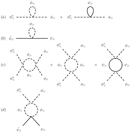
Figure 1: The Feynman graphs contributing to the renormalization of (a) the boson chemical potential $\mu_{b}$, (b)the chemical potential of the low-energy modes of fermions $\delta\mu_{f}$, (c) the boson-boson interaction, and (d) the boson-fermion interaction. Dashed lines denote the boson fields and solid lines denote the fermion fields.

After the integration over the fast fields we perform the scaling transformations $q^{\prime}\rightarrow sq$, $k^{\prime}\rightarrow s^{2}k$, $b^{\prime}(\vec{q}^{\prime}_{i},\omega^{\prime}_{n})\rightarrow s^{(-D-2)/2}b(\vec{q}_{i},\omega_{n})$ and $f^{\prime}(\vec{k}^{\prime}_{i},\omega^{\prime}_{n})\rightarrow s^{-2}f(\vec{k}_{i},\omega_{n})$, which bring the cutoff $\Lambda/s$ back to $\Lambda$. To keep the action invariant under renormalization transformation one finds that the chemical potentials and the coupling constants scale according to the following relations up to one-loop order.

$$\mu_{b}\rightarrow s^{2}\bigg{\{}\mu_{b}-2g_{1}\int^{\Lambda_{b}}_{\Lambda_{b}/s}\frac{d^{D}q}{(2\pi)^{D}}N_{B}(\epsilon_{q}-\mu_{b})$$ (97)

$$-g_{2}\frac{\Omega^{D}K^{D-1}_{F}}{(2\pi)^{D}}\int_{\Lambda_{f}/s^{2}<|k|<\Lambda_{f}}dk~{}~{}N_{F}(v_{F}k-\delta\mu_{f})\Bigg{\}},$$

$$\delta\mu_{f}\rightarrow~{}~{}~{}~{}~{}~{}~{}s^{2}\bigg{\{}\delta\mu_{f}-g_{2}\int^{\Lambda_{b}}_{\Lambda_{b}/s}\frac{d^{D}q}{(2\pi)^{D}}N_{B}(\epsilon_{q}-\mu_{b})\Bigg{\}},$$ (99)

$$g_{1}\rightarrow s^{2-D}\Bigg{\{}g_{1}-g^{2}_{1}\int^{\Lambda_{b}}_{\Lambda_{b}/s}\frac{d^{D}q}{(2\pi)^{D}}\Big{[}4\beta N_{B}(\epsilon_{q}-\mu_{b})$$ (103)

$$\cdot(N_{B}(\epsilon_{q}-\mu_{b})+1)+\frac{1+2N_{B}(\epsilon_{q}-\mu_{b})}{2(\epsilon_{q}-\mu_{b})}\Big{]}$$

$$+g^{2}_{2}\frac{\Omega^{D}K^{D-1}_{F}}{(2\pi)^{D}}\int_{\Lambda_{f}/s^{2}<|k|<\Lambda_{f}}dk~{}~{}\beta N_{F}(v_{F}k-\delta\mu_{f})$$

$$\cdot(N_{F}(v_{F}k-\delta\mu_{f})-1)\Bigg{\}},$$

$$g_{2}\rightarrow s^{2-D}\Bigg{\{}g_{2}-2g_{1}g_{2}\int^{\Lambda_{b}}_{\Lambda_{b}/s}\frac{d^{D}q}{(2\pi)^{D}}\beta N_{B}(\epsilon_{q}-\mu_{b})$$ (105)

$$\cdot(N_{B}(\epsilon_{q}-\mu_{b})+1)\Bigg{\}},$$

where

$$N_{B}(\epsilon_{q}-\mu_{b})=\frac{1}{e^{\beta(\epsilon_{q}-\mu_{b})}-1}$$ (106)

and

$$N_{F}(v_{F}k-\delta\mu_{f})=\frac{1}{e^{(v_{F}k-\delta\mu_{f})}+1}$$ (107)

are the Bose-Einstein and Fermi-Dirac distribution functions which result from the summation over the Matsubara frequencies $\omega_{n}^{b}$ and $\omega^{f}_{n}$ and $\Omega^{D}$ is the D-dimensional solid angle. setting $s=e^{\ell}$ and $\Lambda_{b}(0)=\Lambda_{f}(0)=\Lambda$, we obtain the Gell-Mann-Low equations:

$$\frac{d\mu_{b}}{d\ell}= 2\mu_{b}-2g_{1}\frac{\Omega^{D}\Lambda^{D}}{(2\pi)^{D}}N_{B}(\epsilon_{\Lambda}-\mu_{b})$$ (110)

$$-g_{2}\frac{\Omega^{D}K^{D-1}_{F}\cdot 2\Lambda}{(2\pi)^{D}}\Big{(}N_{F}(-v_{F}\Lambda-\delta\mu_{f})$$

$$+N_{F}(v_{F}\Lambda-\delta\mu_{f})\Big{)},$$

$$\frac{d\delta\mu_{f}}{d\ell}=~{}~{}~{}~{}~{}~{}~{}~{}2\delta\mu_{f}-g_{2}\frac{\Omega^{D}\Lambda^{D}}{(2\pi)^{D}}N_{B}(\epsilon_{\Lambda}-\mu_{b}),$$ (111)

$$~{}~{}~{}\frac{dg_{1}}{d\ell}= (2-D)g_{1}$$ (117)

$$-g^{2}_{1}\frac{\Omega^{D}\Lambda^{D}}{(2\pi)^{D}}\Big{[}4\beta N_{B}(\epsilon_{\Lambda}-\mu_{b})$$

$$\cdot[N_{B}(\epsilon_{\Lambda}-\mu_{b})+1]+\frac{1+2N_{B}(\epsilon_{\Lambda}-\mu_{b})}{2(\epsilon_{\Lambda}-\mu_{b})}\Big{]}$$

$$+g^{2}_{2}\frac{\Omega^{D}K^{D-1}_{F}\cdot 2\Lambda}{(2\pi)^{D}}\beta\Big{[}N_{F}(-v_{F}\Lambda-\delta\mu_{f})$$

$$\cdot[N_{F}(-v_{F}\Lambda-\delta\mu_{f})-1]$$

$$+N_{F}(v_{F}\Lambda-\delta\mu_{f})[N_{F}(v_{F}\Lambda-\delta\mu_{f})-1]\Big{]},$$

$$\frac{dg_{2}}{d\ell}= (2-D)g_{2}-2g_{1}g_{2}\frac{\Omega^{D}\Lambda^{D}}{(2\pi)^{D}}$$ (120)

$$\cdot\beta N_{B}(\epsilon_{\Lambda}-\mu_{b})[N_{B}(\epsilon_{\Lambda}-\mu_{b})+1],$$

$$~{}~{}~{}~{}~{}~{}~{}~{}~{}~{}~{}~{}\frac{d\beta}{d\ell}=~{}~{}~{}~{}-2\beta,~{}~{}~{}~{}~{}~{}~{}~{}~{}~{}~{}~{}~{}~{}~{}~{}~{}~{}~{}~{}~{}~{}~{}~{}~{}~{}~{}~{}~{}~{}~{}~{}~{}~{}~{}~{}~{}~{}~{}~{}~{}~{}~{}~{}~{}~{}~{}~{}~{}~{}$$ (122)

where $\epsilon_{\Lambda}=\frac{\Lambda^{2}}{2m_{b}}$. Eq.(55) $\frac{d\beta}{d\ell}=-2\beta$ shows that for large $\ell$ the temperature $T(\ell)$ always flows to infinity for nonzero initial temperature. This means in the vicinity of the critical point the Bose distribution and Fermi distribution can be reduced as

$$N_{B}(\epsilon_{\Lambda}-\mu_{b})\simeq\frac{1}{\beta(\epsilon_{\Lambda}-\mu_{b})}=\frac{k_{B}Te^{2\ell}}{\epsilon_{\Lambda}-\mu_{b}},$$ (123)

$$N_{F}(v_{F}\Lambda-\delta\mu_{f})\simeq\frac{1}{\beta(v_{F}\Lambda-\delta\mu_{f})+2}\simeq\frac{1}{2}.$$ (124)

To absorb the factor $e^{2\ell}$ in the Eq.(56) we redefine the scaling of the interaction coupling constants in Eq.(51)-(55) as $g_{1}(\ell)=e^{(4-D)\ell}g_{1}$ and $g_{2}(\ell)=e^{(4-D)\ell}g_{2}$. Then the Gell-Mann-Low equations are approximated as:

$$\frac{d\mu_{b}}{d\ell}= 2\mu_{b}-2g_{1}\frac{\Omega^{D}\Lambda^{D}}{(2\pi)^{D}}\cdot\frac{k_{B}T}{\epsilon_{\Lambda}-\mu_{b}}$$ (126)

$$-g_{2}\cdot e^{-2\ell}\cdot\frac{\Omega^{D}K^{D-1}_{F}\cdot 2\Lambda}{(2\pi)^{D}},$$

$$\frac{d\delta\mu_{f}}{d\ell}=~{}~{}~{}~{}~{}~{}~{}~{}2\delta\mu_{f}-g_{2}\frac{\Omega^{D}\Lambda^{D}}{(2\pi)^{D}}\frac{k_{B}T}{\epsilon_{\Lambda}-\mu_{b}},$$ (127)

$$\frac{dg_{1}}{d\ell}= (4-D)g_{1}-g^{2}_{1}\frac{\Omega^{D}\Lambda^{D}}{(2\pi)^{D}}\cdot\frac{5k_{B}T}{(\epsilon_{\Lambda}-\mu_{b})^{2}}$$ (129)

$$-g^{2}_{2}\cdot e^{-4\ell}\frac{\Omega^{D}K^{D-1}_{F}\cdot\Lambda}{(2\pi)^{D}\cdot k_{B}T},$$

$$\frac{dg_{2}}{d\ell}= (4-D)g_{2}-2g_{1}g_{2}\frac{\Omega^{D}\Lambda^{D}}{(2\pi)^{D}}$$ (131)

$$\cdot\frac{k_{B}T}{(\epsilon_{\Lambda}-\mu_{b})^{2}}.$$

We observe that the contributions of the fermion loops go to zero as $\ell\rightarrow\infty$ in above equations because of the factor $e^{-2\ell}$ and $e^{-4\ell}$. Hence, in the vicinity of the critical point we can ignore these contributions. If we redefine the chemical potentials and the coupling constants as

$$\tilde{\mu}_{b}=\mu_{b}/\alpha,$$ (133)

$$\tilde{\delta\mu}_{f}=\delta\mu_{b}/\alpha,$$ (134)

$$\tilde{g}_{1}=g_{1}/\gamma,$$ (135)

$$\tilde{g}_{2}=g_{2}/\gamma,$$ (136)

where $\alpha=\frac{\Lambda^{2}}{m}$ and $\gamma=\frac{(2\pi)^{D}\alpha^{2}}{k_{B}T\Omega^{D}\Lambda^{D}}$, the the Gell-Mann-Low equations can be further simplified as:

$$\frac{d\tilde{\mu}_{b}}{d\ell}= 2\tilde{\mu}_{b}-2\tilde{g}_{1}\cdot\frac{1}{1/2-\tilde{\mu}_{b}},$$ (137)

$$\frac{d\tilde{\delta\mu}_{f}}{d\ell}=~{}~{}~{}~{}~{}~{}~{}~{}2\tilde{\delta\mu}_{f}-\tilde{g}_{2}\cdot\frac{1}{1/2-\tilde{\mu}_{b}},$$ (138)

$$\frac{d\tilde{g}_{1}}{d\ell}= (4-D)\tilde{g}_{1}-\tilde{g}^{2}_{1}\cdot\frac{5}{(1/2-\tilde{\mu}_{b})^{2}},$$ (139)

$$\frac{d\tilde{g}_{2}}{d\ell}= (4-D)\tilde{g}_{2}-2\tilde{g}_{1}\cdot\tilde{g}_{2}\cdot\frac{1}{(1/2-\tilde{\mu}_{b})^{2}}.$$ (141)

The first terms on the right-hand side of Eq.(63)- Eq.(66) are from the tree level scalings. Notice that the tree level scalings of the coupling constants $g_{1}$ and $g_{2}$ go as $4-D$ instead of $2-D$. This is because that near a classical critical point the quantum theory reduces to the classical theory. The same situation has been discussed by reference[28].

Figure 2: Flow diagram of the running coupling constants $\tilde{g}_{1}$ and $\tilde{g}_{2}$ in 3 dimensional case.

For instance, we consider the 3 dimensional case. The fixed points can be calculated as

$$(\tilde{\mu}_{b},\tilde{\delta\mu}_{f},\tilde{g}_{1},\tilde{g}_{2})=(0,0,0,0),$$ (143)

and

$$(\tilde{\mu}_{b},\tilde{\delta\mu}_{f},\tilde{g}_{1},\tilde{g}_{2})=(\frac{1}{12},0,\frac{5}{144},0).$$ (144)

The first one is the trivial Gaussian fixed point and the second one is the Wilson-Fisher fixed point. Around the Wilson-Fisher fixed point, the running of the two coupling constants are shown in the flow diagram Fig.2. We can see that with a small negative initial value the coupling constant $\tilde{g}_{2}$ runs to negative infinity. This could indicate a boson-fermion pairing instability.

4 Conclusion

In this paper we investigated a weakly interacting boson-fermion mixture model by application of Wilson’s renormalization group analysis. This model includes one boson-boson interaction coupling constant $g_{1}$ and one boson-fermion interaction coupling constant $g_{2}$. At tree level RG analysis shows that the scaling dimensions of $g_{1}$ and $g_{2}$ are both $2-D$. That is, the two coupling constants are marginal in $D=2$. Here one needs to notice that the derivation of the scaling dimension of $g_{2}$ is under a condition of Eq.(34), without which we won’t be able to compare the rescaled action with the original one in RG transformation.

At one-loop level we derived the Gell-Mann-Low equations and found that in these equations the contributions from the fermion loops went to zero exponentially as $\ell\rightarrow\infty$ compared with the contributions of the boson loops. We simplify these Gell-Mann Low equations by ignoring the fermion loop contributions and solve for fixed points in 3 dimensional case as an example. We found two fixed points. One is the trivial Gaussian fixed point and the other one is the Wilson-Fisher fixed point at which $g_{2}$ vanishes. This implies that the boson-fermion interaction decouples at the critical temperature. We also drew the flow diagram of the coupling constants $g_{1}$ and $g_{2}$ around the Wilson-Fisher fixed point. We observe that $g_{2}$ goes to negative infinity with a small negative initial value. This can be a boson-fermion pairing instability.

Supersymmetry is a symmetry that relates boson and fermion. It has been one of the most active research areas in the high energy physics[30]. Various researches were also conducted to find supersymmetry in condensed matter systems[7, 8]. If we have $\mu_{b}=\mu_{f}=\mu$ and $g_{1}=g_{2}=g$ in Eq.(2), we can combine the boson and fermion field as a doublet $\Phi=\left(\begin{array}[]{c}\phi\\ \psi\end{array}\right)$, which is called superfield. Then the action can be rewrite in terms of superfield as

$$S[\Phi^{\dagger},\Phi]= \int d^{D}x\int^{\beta}_{0}d\tau\Big{\{}\Phi^{\dagger}(\partial_{\tau}-\frac{\hbar^{2}}{2m_{b}}\nabla^{2}-\mu)\Phi$$ (146)

$$+\frac{g}{2}(\Phi^{\dagger}\Phi)^{2}\Big{\}}.$$

This action is invariant under supergroup $U(1|1)$[13]. We used renormalization group method to explore if there is a supersymmetry fixed point where $\mu_{b}=\mu_{f}$ and $g_{1}=g_{2}$. The calculation of the Gell-Mann Low equations shows that our model doesn’t exhibit such a fixed point.

Acknowledgements

It’s a pleasure to thank Professor Wei-Feng Tsai and Dr. Chi Xiong for useful discussions.

References

[1]M. H. Anderson et al., Science 269, 198 (1995); K. B.
Davis et al., Phys. Rev. Lett. 75, 3969 (1995).
[2] A. Storozhenko, P. Schuck, T. Suzuki, H. Yabu and J.
Dukelsky, Phys. Rev. A 71, 063617 (2005).
[3]T. Miyakawa, T. Suzuki, and H. Yabu, Phys. Rev. A 64,
033611 (2001).
[4]R. Roth, Phys. Rev. A 66, 013614 (2002).
[5] T. Tsurumi and M. Wadati, J. Phys. Soc. Jpn. 69, 97 (2000).
[6] C. J. Pethick and H. Smith, Bose-Einstein Condensation in
Dilute Gases, (Cambridge University Press, Cambridge, U.K., 2002).
[7] M. Snoek, M. Haque, S. Vandoren and H. T. C.
Stoof, Phys. Rev. Lett. 95, 250401 (2005); M. Snoek, S.
Vandoren, and H. T. C. Stoof, Phys. Rev. A 74, 033607
(2006).
[8]Y. Yu and K. Yang, Phys. Rev. Lett. 100, 090404
(2008); T. Shi, Yue Yu, and C. P. Sun, Phys. Rev. A 81,
011604 (2010).
[9]G. Modugno, G. Roati, F. Riboli, F. Ferlaino, R. J. Brecha, and
M. Inguscio, Science 297, 2240 (2002).
[10]C. Ospelkaus, S. Ospelkaus, L. Humbert, P. Ernst, K. Sengstock, and K. Bongs, Phys. Rev. Lett.
97, 120402 (2006).
[11]J. J. Zirbel, K. -K. Ni, S. Ospelkaus, J. P. D’Incao, C. E. Wieman, J. Ye, and D. S. Jin, Phys.
Rev. Lett. 100, 143201 (2008).
[12] Sung-Sik Lee, Phys. Rev. B 76, 075103 (2007).
[13] I. Bars, Lect. Appl. Math. 21, 17, (1983).
[14] K. G. Wilson and J. B. Kogut, Phys. Rep. 12, 75 (1974).
[15] J. A. Hertz, Phys. Rev. B 14, 1165 (1976).
[16] E. B. Kolomeisky and J. P. Straley, Phys. Rev. B 46, 11749
(1992).
[17] E. B. Kolomeisky and J. P. Straley, Phys. Rev. B 46, 13942
(1992).
[18] M. Bijlsma and H. T. S. Stoof, Phys. Rev. A 54, 5085 1996.
[19] J. Feldman and E. Trubowitz, Helv. Phys. Acta. 63, 156 (1990).
[20] G. Benfatto and G. Gallavotti, Phys. Rev. B 42, 9967 (1990).
[21] R. Shankar, Physica A 177, 530 (1991).
[22] R. Shankar, Rev. Mod. Phys. 66, 129 (1994).
[23] J. Polchinski, Nucl. Phys. B 422, 617 (1994).
[24] C. Nayak and F. Wilczek, Nucl. Phys. B 430, 534 (1994).
[25] M. Onoda, I. Ichinose, and T. Matsui, Nucl. Phys. B 446, 353
(1995).
[26] N. Furukawa, T. M. Rice, and M. Salmhofer, Phys. Rev. Lett.
81, 3195 (1998).
[27] Seiji J. Yamamoto and Qimiao Si, Phys. Rev. B
81, 205106 (2010).
[28]Henk T. C. Stoof, Dennis B. M. Dickerscheid and Koos
Gubbels, Ultracold Quantum Fields, Springer, 2009, Page 345.