Polaronic properties of an impurity in a Bose-Einstein condensate in reduced dimensions.

Abstract

The application of optical lattices allows a tuning of the geometry of Bose-Einstein condensates to effectively reduced dimensions. In the context of solid state physics the consideration of the low-dimensional Fröhlich polaron results in an extension of the polaronic strong coupling regime. With this motivation we apply the Jensen-Feynman variational principle to calculate the ground state properties of the polaron consisting of an impurity in a Bose-Einstein condensate in reduced dimensions. Also the response of this system to Bragg scattering is calculated. We show that reducing the dimension leads to a larger amplitude of the polaronic features and is expected to facilitate the experimental observation of polaronic properties. In optical lattices not only Feshbach resonances but also confinement-induced resonances can be used to tune the polaronic coupling strength. This opens up the possibility to experimentally reveal the intermediate and strong polaronic coupling regimes and resolve outstanding theoretical questions regarding polaron theory.

I Introduction

In recent years ultracold atomic systems have revealed themselves as quantum simulators for many-body theories RevModPhys.80.885 . Especially their high degree of tunability makes them attractive for this purpose. An example of a system that can be simulated in this way is the Fröhlich polaron which is well-known from solid state physics where it is used to describe charge carriers in a polar solid (see for example Ref. BoekDevreese for an extended overview). In the context of ultracold gases the system of impurities embedded in a Bose-Einstein condensation can be mapped onto the Fröhlich polaron Hamiltonian PhysRevLett.96.210401 ; PhysRevA.73.063604 . In this case the role of the charge carriers is played by the impurities and the lattice vibrations are replaced by the Bogoliubov excitations. Recently this system has gained much interest both theoretically PhysRevA.76.011605 ; 1367-2630-10-3-033015 ; 0295-5075-82-3-30004 ; PhysRevA.82.063614 ; 1367-2630-13-10-103029 ; PhysRevB.80.184504 ; springerlink:10.1134/S1054660X11150035 ; PhysRevA.84.063612 ; PhysRevA.83.033631 ; springerlink:10.1007/s10909-010-0286-0  and experimentally springerlink:10.1007/s00340-011-4868-6 ; PhysRevLett.105.133202 ; PhysRevA.77.011603 ; PhysRevLett.105.045303 ; 2011arXiv1106.0828C .

For the present work we focus on a single Fröhlich polaron for which the Hamiltonian can not be analytically diagonalized and one has to rely on approximation methods. The most advanced theory for the ground state properties is the Jensen-Feynman variational principle PhysRev.97.660 which can be extended through the Feynman-Hellwarth-Iddings-Platzman (FHIP) approximation for the response properties PhysRev.127.1004 ; PhysRevB.5.2367 . The optical absorption of the Fröhlich solid state polaron was later also obtained through a diagrammatic Monte Carlo calculation and a comparison with the FHIP approximation showed a good agreement at weak and intermediate polaronic coupling but in the strong coupling regime deviations were revealed PhysRevLett.91.236401 ; PhysRevLett.96.136405 . Since there is no known material that exhibits the strong coupling behavior only the weak and intermediate coupling regime could be experimentally probed which resulted in a good agreement with the theory PolaronsAndExcitons ; PhysRevLett.58.1471 . A better understanding of the strong coupling regime could also shed light on the possible role of polarons and bipolarons in unconventional pairing mechanisms for high-temperature superconductivity BoekAlexandrov ; PhysRevB.77.094502 . Recently it was shown that for an impurity in a condensate the use of a Feshbach resonance allows an external tuning of the polaronic coupling parameter which makes it a promising system to probe the strong polaronic coupling regime for the first time PhysRevB.80.184504 . Recent experiments have shown the feasibility of using Feshbach resonances for the tuning of interparticle interactions between different species PhysRevA.85.042721 ; PhysRevA.85.032506 ; PhysRevA.85.051602 .

Since the impurities are considered as not charged it is not possible to conduct optical absorption measurements to reveal the polaronic excitation structure as is possible for the Fröhlich solid state polaron. It was shown in PhysRevA.83.033631 that Bragg spectroscopy is suited to experimentally probe the polaronic excitation structure of an impurity in a condensate. Bragg scattering is a well established experimental technique in the context of ultracold gases (see for example Refs. PhysRevLett.88.120407 ; PhysRevLett.83.2876 ). The setup consists of two laser beams with different frequencies $\omega_{1}$ and $\omega_{2}$ and different momenta $\vec{k}_{1}$ and $\vec{k}_{2}$ that are radiated on the impurity. The impurity can then absorb a photon from laser 1 and emit it to laser 2 during which process it has gained an energy $\omega=\omega_{1}-\omega_{2}$ and a momentum $\vec{k}=\vec{k}_{1}-\vec{k}_{2}$. The response is reflected in the number of impurities that have gained a momentum $\vec{k}$ as a function of $\vec{k}$ and $\omega$. This number is proportional to the imaginary part of the density response function $\chi\left(\omega,\vec{k}\right)$ Pitaevskii :

$$\chi\left(\omega,\vec{k}\right)=\frac{i}{\hbar}\int_{0}^{\infty}dte^{i\omega t}\left\langle\left[\widehat{\rho}_{\vec{k}}\left(t\right),\widehat{\rho}_{\vec{k}}^{{\dagger}}\right]\right\rangle,$$ (1)

with $\widehat{\rho}_{\vec{k}}$ the density operator of the impurity.

Another powerful tool in the context of ultracold gases is the application of optical lattices which can be employed to modify the geometry of the system citeulike:2749190 . This allows to confine the system in one or two directions such that the confinement length is much smaller than all other typical length scales which results in an effectively low dimensional system. For these systems the interparticle interactions can be described through a contact pseudopotential with an amplitude that is a function of the three-dimensional scattering length and the confinement length. This permits to experimentally tune the interactions between the particles by varying the strength of the confinement which results in a resonant behavior. These confinement-induced resonances have been studied both theoretically PhysRevLett.101.170401 ; 1367-2630-7-1-192 ; PhysRevLett.91.163201 ; PhysRevLett.81.938 ; PhysRevA.64.012706 and experimentally PhysRevLett.104.153203 ; PhysRevLett.94.210401 ; Haller04092009 ; PhysRevLett.104.153202 ; PhysRevLett.106.105301 .

In the present work we adapt the calculations of the ground state and response properties of the polaronic system consisting of an impurity in a condensate to the case of reduced dimensions. This was done for the Fröhlich solid state polaron in Refs. PhysRevB.33.3926 ; PhysRevB.31.3420 ; PhysRevB.36.4442  which led to the polaronic scaling relations. These are applicable for polaronic systems of which the interaction amplitude $V_{\vec{k}}$ (see later) is a homogeneous function. Unfortunately this is not the case for the polaron consisting of an impurity in a Bose-Einstein condensate. We start by showing that also in lower dimensions the Hamiltonian of an impurity in a condensate can be mapped onto the Fröhlich polaron Hamiltonian. Then the Jensen-Feynman variational principle is applied to calculate an upper bound for the free energy and an estimation of the effective mass and the radius of the polaron as was done in Ref. PhysRevB.80.184504  for the three-dimensional case. Subsequently the treatment of Ref. PhysRevA.83.033631 for the response to Bragg spectroscopy in 3 dimensions is adapted to reduced dimensions. All results are applied to the specific system of a lithium-6 impurity in a sodium condensate.

II Impurity in a condensate in $d$ dimensions

The Hamiltonian of an impurity in an interacting bosonic gas is given by:

$$\widetilde{H}=\frac{\widehat{p}^{2}}{2m_{I}}+\sum_{\vec{k}}E_{\vec{k}}\widehat{a}_{\vec{k}}^{{\dagger}}\widehat{a}_{\vec{k}}+\frac{1}{2}\sum_{\vec{k},\vec{k}^{\prime},\vec{q}}V_{BB}\left(\vec{q}\right)\widehat{a}_{\vec{k}^{\prime}-\vec{q}}^{{\dagger}}\widehat{a}_{\vec{k}+\vec{q}}^{{\dagger}}\widehat{a}_{\vec{k}}\widehat{a}_{\vec{k}^{\prime}}+\sum_{\vec{k},\vec{q}}V_{IB}\left(\vec{q}\right)e^{i\vec{q}.\widehat{r}}\widehat{a}_{\vec{k}^{\prime}-\vec{q}}^{{\dagger}}\widehat{a}_{\vec{k}^{\prime}}.$$ (2)

The first term in this expression represent the kinetic energy of the impurity with $\widehat{p}$ ($\widehat{r}$) the momentum (position) operator of the impurity with mass $m_{I}$. The second term in the right-hand side of (2) describes the kinetic energy of the bosons with creation (annihilation) operators $\left\{\widehat{a}_{\vec{k}}^{{\dagger}}\right\}$ ($\left\{\widehat{a}_{\vec{k}}\right\}$) and energy $E_{\vec{k}}=\frac{\hbar^{2}k^{2}}{2m_{B}}-\mu$ where $\mu$ is the chemical potential of the bosons and $m_{B}$ their mass. The last two terms represent the interaction energy with $V_{BB}\left(\vec{q}\right)$ the Fourier transform of the boson-boson interaction potential and $V_{IB}\left(\vec{q}\right)$ of the impurity-boson interaction potential. All vectors in expression (2) are considered as $d$-dimensional.

In Refs. PhysRevLett.85.3745 and PhysRevLett.84.2551 it is shown that in one and two dimensions, respectively, at temperatures well below a critical temperature $T_{c}$ a trapped weakly interacting Bose gas is characterized by the presence of a true condensate while just below $T_{c}$ this is a quasicondensate. A quasicondensate exhibits phase fluctuations with a radius $R_{\phi}$ that is smaller than the size of the system but greatly exceeds the coherence length $\xi$ PhysRevLett.85.3745 ; PhysRevLett.84.2551 . Since the radius of the polaron $R_{pol}$ is typically of the order $\xi$ (see later) we have $R_{pol}\ll R_{\phi}$ which shows that the polaronic features are also present in a quasicondensate. In the following we no longer make the distinction and use the name condensate for both situations. The presence of a condensate can be expressed through the Bogoliubov shift which (within the local density aproximation) transforms the Hamiltonian (2) into PhysRevB.80.184504 :

$$\widehat{H}=E_{GP}+g_{IB}N_{0}+\widehat{H}_{pol},$$ (3)

where use was made of contact interactions, i.e. $V_{BB}\left(\vec{q}\right)=g_{BB}$ and $V_{IB}\left(\vec{q}\right)=g_{IB}$. In order to have a stable condensate the boson-boson interaction should be repulsive, i.e. $g_{BB}>0$. The sign of the impurity-boson interaction strength $g_{IB}$ is in priciple arbitrary, however for the Bogoliubov approximation to be valid the depletion of the condensate around the impurity must remain smaller than the condensate density which means the formalism is not valid for a large negative $g_{IB}$ 0295-5075-82-3-30004 ; PhysRevLett.102.030408 . The first term in the right-hand side of (3) represents the Gross Pitaevskii energy $E_{GP}$ of the condensate and the second term gives the interaction of the impurity with the condensate (with $N_{0}$ the number of condensed bosons in a unit volume). The third term is the polaron Hamiltonian which describes the interaction between the impurity and the Bogoliubov excitations:

$$\widehat{H}_{pol}=\frac{\widehat{p}^{2}}{2m_{I}}+\sum_{\vec{k}\neq 0}\hbar\omega_{\vec{k}}\widehat{\alpha}_{\vec{k}}^{{\dagger}}\widehat{\alpha}_{\vec{k}}+\sum_{\vec{k}\neq 0}V_{\vec{k}}\rho_{I}\left(\vec{k}\right)\left(\widehat{\alpha}_{\vec{k}}+\widehat{\alpha}_{-\vec{k}}^{{\dagger}}\right),$$ (4)

where $\left\{\widehat{\alpha}_{\vec{k}}^{{\dagger}}\right\}$ ($\left\{\widehat{\alpha}_{\vec{k}}\right\}$) are the creation (annihilation) operators of the Bogoliubov excitations with dispersion:

$$\hbar\omega_{\vec{k}}=\frac{\hbar^{2}k}{2m_{B}\xi}\sqrt{\left(\xi k\right)^{2}+2},$$ (5)

with $\xi$ the healing length: $\xi=\sqrt{\frac{\hbar^{2}}{2m_{B}N_{0}g_{BB}}}$. The interaction amplitude $V_{\vec{k}}$ is given by:

$$V_{\vec{k}}=\sqrt{N_{0}}g_{IB}\left(\frac{\left(\xi k\right)^{2}}{\left(\xi k\right)^{2}+2}\right)^{1/4}.$$ (6)

III Polaronic ground state properties in $d$ dimensions

In this section we summarize the main results from standard polaron theory regarding the ground state properties with emphasis on the dependency on the dimension (see for example Ref. 2010arXiv1012.4576D for more details) and we apply this to the polaronic system consisting of an impurity in a condensate.

III.1 Jensen-Feynman variational principle

The most accurate available description of the ground state properties of a polaron is based on the Jensen-Feynman inequality which states PhysRev.97.660 ; BoekFeynman :

$$\mathcal{F}\leq\mathcal{F}_{0}+\frac{1}{\hbar\beta}\left\langle\mathcal{S-S}_{0}\right\rangle_{\mathcal{S}_{0}},$$ (7)

with $\mathcal{F}$ the free energy of the system, $\mathcal{F}_{0}$ the free energy of a trial system, $\beta=\left(k_{B}T\right)^{-1}$ the inverse temperature with $k_{B}$ the Boltzmann constant,$\ \mathcal{S}$ the action of the system and $\mathcal{S}_{0}$ the action of the trial system. It was suggested by Feynman to consider the particle harmonically coupled to a mass $M$ with a coupling constant $MW^{2}$ for the trial system PhysRev.97.660 . This leads to the following expression for the Jensen-Feynman inequality (7) PhysRevB.33.3926 :

$$\mathcal{F} \leq\frac{d}{\beta}\left\{\ln\left[2\sinh\left(\frac{\beta\hbar\Omega}{2}\right)\right]-\ln\left[2\sinh\left(\frac{\beta\hbar\Omega}{2\sqrt{1+M/m}}\right)\right]\right\}$$

$$-\frac{1}{\beta}\ln\left[V\left(\frac{m+M}{2\pi\hbar^{2}\beta}\right)^{d/2}\right]-\frac{d}{2\beta}\frac{M}{m+M}\left[\frac{\hbar\beta\Omega}{2}\coth\left[\frac{\hbar\beta\Omega}{2}\right]-1\right]$$

$$-\sum_{\vec{k}}\frac{\left|V_{\vec{k}}\right|^{2}}{\hbar}\int_{0}^{\hbar\beta/2}du\mathcal{G}\left(\vec{k},u\right)\mathcal{M}_{M,\Omega}\left(\vec{k},u\right),$$ (8)

with $d$ the dimension, $V$ the volume, $\Omega=W\sqrt{1+M/m_{I}}$ and $\mathcal{G}\left(\vec{k},u\right)$ the Green function of the Bogoliubov excitations:

$$\mathcal{G}\left(\vec{k},u\right)=\frac{\cosh\left[\omega_{\vec{k}}\left(u-\hbar\beta/2\right)\right]}{\sinh\left[\hbar\beta\omega_{\vec{k}}/2\right]},$$ (9)

and $\mathcal{M}_{M,\Omega}\left(\vec{k},u\right)$ the memory function:

$$\mathcal{M}_{M,\Omega}\left(\vec{k},u\right)=\exp\left[-\frac{\hbar k^{2}}{2\left(m+M\right)}\left\{u-\frac{u^{2}}{\hbar\beta}-\frac{M}{m}\frac{\cosh\left[\Omega\hbar\beta/2\right]-\cosh\left[\Omega\left(\hbar\beta/2-u\right)\right]}{\Omega\sinh\left(\hbar\beta\Omega/2\right)}\right\}\right].$$ (10)

The parameters $\Omega$ and $M$ are then determined variationally by minimizing the expression (8). The present treatment also allows an estimation of the radius of the polaron as the root mean square of the reduced coordinate $\vec{r}$ of the model system PhysRevB.31.4890 :

$$\left\langle r^{2}\right\rangle=d\frac{\hbar}{2\Omega}\frac{m_{I}+M}{Mm_{I}}\coth\left(\frac{\beta\hbar\Omega}{2}\right).$$ (11)

In PhysRev.97.660 Feynman also presented a calculation of the polaronic effective mass $m^{\ast}$ at zero temperature:

$$m^{\ast}=m_{I}+\frac{1}{d}\sum_{\vec{k}}k^{2}\frac{\left|V_{\vec{k}}\right|^{2}}{\hbar}\int_{0}^{\infty}due^{-\omega_{\vec{k}}u}\mathcal{F}_{M,\Omega}\left(\vec{k},u\right)u^{2},$$ (12)

with:

$$\mathcal{F}_{M,\Omega}\left(\vec{k},u\right)=\lim_{\beta\rightarrow\infty}\mathcal{M}_{M,\Omega}\left(\vec{k},u\right)=\exp\left\{-\frac{\hbar k^{2}}{2\left(m+M\right)\Omega}\left[\frac{M}{m}\left(1-e^{-\Omega u}\right)+\Omega u\right]\right\}.$$ (13)

As far as we know there exists no generalization of equation (12) to finite temperatures but as a first estimation we use (12) with the temperature dependent variational parameters $M$ and $\Omega$.

III.2 Polaron consisting of an impurity in a condensate

Here we introduce the Bogoliubov spectrum (5) and the interaction amplitude (6) which are specific for the polaronic system consisting of an impurity in a condensate. This allows us to write the Jensen-Feynman inequality (8) as (we also use polaronic units, i.e. $\hbar=\xi=m_{I}=1$):

$$\mathcal{F} \leq\frac{d}{\beta}\left\{\ln\left[2\sinh\left(\frac{\beta\Omega}{2}\right)\right]-\ln\left[2\sinh\left(\frac{\beta\Omega}{2\sqrt{1+M}}\right)\right]\right\}$$

$$-\frac{1}{\beta}\ln\left[V\left(\frac{1+M}{2\pi\beta}\right)^{d/2}\right]-\frac{d}{2\beta}\frac{M}{1+M}\left[\frac{\beta\Omega}{2}\coth\left[\frac{\beta\Omega}{2}\right]-1\right]$$

$$-\frac{\alpha^{\left(d\right)}}{4\pi}\left(\frac{m_{B}+1}{m_{B}}\right)^{2}\int_{0}^{\infty}dk\frac{k^{d}}{\sqrt{k^{2}+2}}\int_{0}^{\beta/2}du\mathcal{G}\left(k,u\right)\mathcal{M}_{M,\Omega}\left(k,u\right),$$ (14)

where we introduced the dimensionless coupling parameter $\alpha^{\left(d\right)}$ as follows:

$$\alpha^{\left(d\right)}=4\pi\frac{2\pi^{d/2}}{\Gamma\left(\frac{d}{2}\right)}N_{0}g_{IB}^{2}\left(\frac{m_{I}\xi^{2}}{\hbar^{2}}\right)^{2}\frac{V}{\left(2\pi\xi\right)^{d}}\left(\frac{m_{B}}{m_{B}+m_{I}}\right)^{2},$$ (15)

with $\Gamma\left(x\right)$ the gamma function. The prefactor was chosen to be in agreement with the definition for $\alpha^{\left(3\right)}$ in Ref. PhysRevB.80.184504  . Note that the coupling parameter depends on the impurity-boson interaction amplitude $g_{IB}$ and also on the boson-boson interaction amplitude $g_{BB}$ through the healing length $\xi$. As mentioned in the introduction these interaction amplitudes and thus also the coupling parameter can be externally tuned through a Feshbach resonance or in reduced dimensions also with a confinement induced resonance.

For $d=2$ the $k$-integral in (14) contains an ultraviolet divergence. This is also the case in 3 dimensions and it was shown in Ref. PhysRevB.80.184504 that this is solved by applying the Lippmann-Schwinger equation up to second order for the interaction amplitude in the second term of the Hamiltonian (3). This results in a renormalization factor that is incorporated through the following substitution PhysRevB.80.184504 :

$$N_{0}g_{IB}\rightarrow N_{0}\left(T\left(E\right)+g_{IB}^{2}\sum_{\vec{k}}\frac{1}{\frac{\hbar^{2}k^{2}}{2m_{r}}-E}\right),$$ (16)

with $T\left(E\right)$ the scattering $T$-matrix. In 2 dimensions the limit $E\rightarrow 0$ in (16) results in an infrared divergence. The second term in (16) can be written as:

$$N_{0}g_{IB}^{2}\sum_{\vec{k}}\frac{1}{\frac{\hbar^{2}k^{2}}{2m_{r}}-E}=\frac{\alpha^{\left(2\right)}}{2\pi}\frac{\hbar^{2}}{m_{I}\xi^{2}}\frac{m_{B}+m_{I}}{m_{B}}\int_{0}^{\infty}\frac{k}{k^{2}-2m_{r}E/\hbar^{2}}dk,$$ (17)

which lifts the ultraviolet divergence in (14). For numerical considerations a cutoff $K_{c}$ is introduced for the $k$-integral which enables us to calculate the integral in (17):

$$\frac{\alpha^{\left(2\right)}}{2\pi}\frac{\hbar^{2}}{m_{I}\xi^{2}}\frac{m_{B}+m_{I}}{m_{B}}\int_{0}^{K_{c}}\frac{k}{k^{2}-2m_{r}\xi^{2}E/\hbar^{2}}dk =\frac{\alpha^{\left(2\right)}}{4\pi}\frac{\hbar^{2}}{m_{I}\xi^{2}}\frac{m_{B}+m_{I}}{m_{B}}\ln\left(\frac{\frac{\hbar^{2}K_{c}^{2}}{2m_{r}}-E}{E}\right)$$

$$\approx\frac{\alpha^{\left(2\right)}}{4\pi}\frac{\hbar^{2}}{m_{I}\xi^{2}}\frac{m_{B}+m_{I}}{m_{B}}\ln\left(\frac{\hbar^{2}K_{c}^{2}}{2m_{r}E}\right),$$ (18)

where in the second step we used the fact that the energy related to the cutoff is much larger than the typical energy of the scattering event $E$. Equation (18) shows that the chosen value of $E$ is not important since it only results in an energy shift and therefore has no influence on the physical properties of the system.

III.3 Results

We apply the presented treatment to the system of a lithium-6 impurity in a sodium condensate ($m_{B}/m_{I}=3.82207$). All results are presented in polaronic units, i.e. $\hbar=\xi=m_{I}=1$.

In figure 1 the results for the polaronic ground state properties in 2 dimensions as a function of the coupling parameter $\alpha^{\left(2\right)}$ are presented. In (a) the radius of the polaron is shown and in (b) the effective mass at different temperatures. The observed behavior is analogous to the three-dimensional case (see Ref. PhysRevB.80.184504 ) and suggests that for growing $\alpha^{\left(2\right)}$ the self-induced potential becomes stronger leading to a bound state at high enough $\alpha^{\left(2\right)}$. However, as compared to the three-dimensional case, the transition is much smoother with a transition region between $\alpha^{\left(2\right)}\approx 1$ and $\alpha^{\left(2\right)}\approx 3$. This behavior is in agreement with the mean-field results of Refs. PhysRevB.46.301 ; 0295-5075-82-3-30004 , where also a smooth transition to the self-trapped state was found for $d=2$. For the cutoff $K_{c}$ we used the inverse of the Van der Waals radius for sodium which results in $K_{c}=200$. To check whether this cutoff is large enough the variational parameter $M$ is plotted in the inset of figure (1)(b) for different values of $K_{c}$ which reveals already a reasonable convergence at $K_{c}\approx 5$.

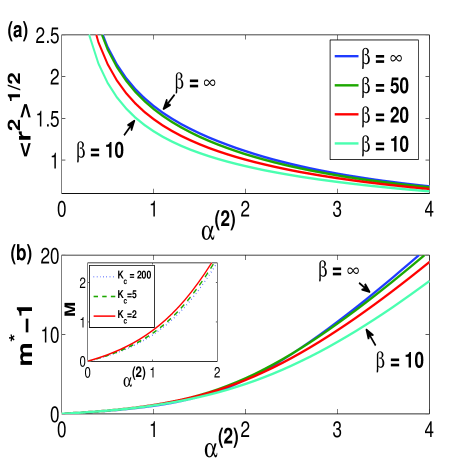
Figure 1: (Color online) The groundstate properties of the polaron consisting of a lithium-6 impurity in a sodium condensate in 2 dimensions. In (a) the radius of the polaron (11) is presented and in (b) the effective mass (12) as a function of the polaronic coupling parameter $\alpha^{\left(2\right)}$ at different temperatures ($\beta=\left(k_{B}T\right)^{-1}$) and with a cutoff $K_{c}=200$. The inset shows the variational parameter $M$ for different values of the cutoff $K_{c}$ at $\beta=50$. All results are presented in polaronic units ($\hbar=m_{I}=\xi=1$).

In figure 2 the results for the 1-dimensional case are presented. In (a) the radius of the polaron is plotted and (b) shows the effective mass at different temperatures. For growing $\alpha^{\left(1\right)}$ the characteristics of the appearance of a bound state in the self-induced potential are again observed. The characteristics of the weak coupling regime are however not present and the transition region is between $\alpha^{\left(1\right)}=0$ and $\alpha^{\left(1\right)}\approx 1$. This is again in agreement with the mean-field results of Refs. PhysRevB.46.301 ; 0295-5075-82-3-30004 for $d=1$.

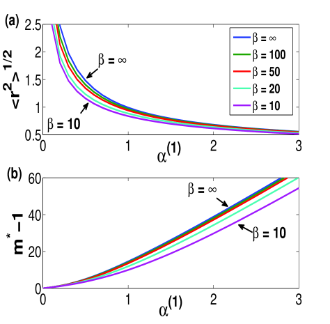
Figure 2: (Color online) The polaronic ground state properties of a lithium-6 impurity in a sodium condensate in 1 dimension. The radius (a) and the effective mass (b) are presented as a function of the polaronic coupling parameter $\alpha^{\left(1\right)}$ at different temperatures ($\beta=\left(k_{B}T\right)^{-1}$). All results are presented in polaronic units ($\hbar=m_{I}=\xi=1$).

IV Response to Bragg scattering in $d$ dimensions

The response of a system to Bragg spectroscopy is proportional to the imaginary part of the density response function (1). In Ref. PhysRevA.83.033631 it was shown that the use of the Feynman-Hellwarth-Iddings-Platzman approximation (as introduced in Ref. PhysRev.127.1004  for a calculation of the impedance of the Fröhlich solid state polaron and generalized in Ref. PhysRevB.5.2367 for the optical absorption) leads to the following expression for the Bragg response:

$$\operatorname{Im}\left[\chi\left(\omega,\vec{k}\right)\right]=-\frac{k^{2}}{m_{I}}\frac{\operatorname{Im}\left[\Sigma\left(\omega,\vec{k}\right)\right]}{\left\{\omega^{2}-\operatorname{Re}\left[\Sigma\left(\omega,\vec{k}\right)\right]\right\}^{2}+\left\{\operatorname{Im}\left[\Sigma\left(\omega,\vec{k}\right)\right]\right\}^{2}},$$ (19)

with $\Sigma\left(\omega,\vec{k}\right)$ the self energy:

$$\Sigma\left(\omega,\vec{k}\right) =\frac{2}{m_{I}N\hbar}\sum_{\vec{q}\neq 0}\left|V_{\vec{q}}\right|^{2}\frac{\left(\vec{k}.\vec{q}\right)^{2}}{k^{2}}$$ (20)

$$\times\int_{0}^{\infty}dt\left(1-e^{i\omega t}\right)\operatorname{Im}\left\{\left[e^{i\omega_{\vec{q}}t}+2\cos\left(\omega_{\vec{q}}t\right)n\left(\omega_{\vec{q}}\right)\right]\exp\left[-\left(\vec{k}+\vec{q}\right)^{2}D\left(t\right)\right]\right\},$$ (21)

$n\left(\omega\right)=\left(\exp\left[\beta\hbar w\right]-1\right)^{-1}$ the Bose-Einstein distribution and:

$$D\left(t\right)=\frac{t^{2}}{2\beta\left(m_{I}+M\right)}-i\frac{\hbar}{2\left(m_{I}+M\right)}t+\frac{\hbar M}{2m_{I}\Omega\left(m_{I}+M\right)}\left[1-e^{i\Omega t}+4\sin^{2}\left(\frac{\Omega t}{2}\right)n\left(\Omega\right)\right].$$ (22)

For numerical calculations the representation for the self energy as derived in appendix A is used.

IV.1 Sum rule

As was first noted in PhysRevB.15.1212 for the Fröhlich polaron and generalized in PhysRevA.83.033631 for an impurity in a condensate the f-sum rule can be written as:

$$\frac{\pi}{2}\frac{1}{\left(1-R\left(\alpha,k\right)\right)}+\frac{m_{I}}{k^{2}}\int_{\varepsilon}^{\infty}d\omega\omega\operatorname{Im}\left[\chi\left(\omega,\vec{k}\right)\right]=\frac{\pi}{2},$$ (23)

with $\varepsilon$ a small number such that the Drude peak (see later) is not included in the integral and:

$$R\left(\alpha,k\right)=\lim_{\omega\rightarrow 0}\frac{\operatorname{Re}\left[\Sigma\left(\omega,\vec{k}\right)\right]}{\omega^{2}}.$$ (24)

In the limits $\beta\rightarrow\infty$ and $k\rightarrow 0$ the function (24) is related to the Feynman effective mass (12) PhysRevB.15.1212 :

$$m^{\ast}=m_{I}\left(1-\lim_{\beta\rightarrow\infty}R\left(\alpha,0\right)\right).$$ (25)

This relation provides a powerful experimental tool to determine the effective mass from the optical response which was recently applied for the Fröhlich solid state polaron PhysRevB.81.125119 ; PhysRevLett.100.226403 .

IV.2 Self energy for an impurity in a condensate

Introducing the interaction amplitude (6) and the coupling parameters (15) in expressions (42) and (45) for the imaginary and real part of the self energy results in (using polaronic units):

$$\operatorname{Im}\left[\Sigma\left(\omega,\vec{k}\right)\right] =\sqrt{2\pi\beta\left(1+M\right)}\frac{\alpha^{\left(d\right)}}{8\pi}\frac{\Gamma\left(d/2\right)}{2\pi^{d/2}}\left(\frac{m_{B}+1}{m_{B}}\right)^{2}B\left(\beta,n,n^{\prime}\right)$$

$$\times\sum_{n,n^{\prime}=0}^{\infty}\int d\vec{q}\frac{q}{\sqrt{q^{2}+2}}\frac{\left(\vec{k}.\vec{q}\right)^{2}}{k^{2}}\left|\vec{k}+\vec{q}\right|^{2\left(n+n^{\prime}\right)-1}e^{-a^{2}\left(\beta\right)\left(\vec{k}+\vec{q}\right)^{2}}$$

$$\times\left\{\left[1+n\left(\omega_{\vec{q}}\right)\right]\left[e^{-\frac{\beta\left(1+M\right)\left(A^{+}+\omega\right)^{2}}{2\left(\vec{k}+\vec{q}\right)^{2}}}-e^{-\frac{\beta\left(1+M\right)\left(A^{+}-\omega\right)^{2}}{2\left(\vec{k}^{\prime}+\vec{q}\right)^{2}}}\right]\right.$$

$$\left.+n\left(\omega_{\vec{q}}\right)\left[e^{-\frac{\beta\left(1+M\right)\left(A^{-}+\omega\right)^{2}}{2\left(\vec{k}+\vec{q}\right)^{2}}}-e^{-\frac{\beta\left(1+M\right)\left(A^{-}-\omega\right)^{2}}{2\left(\vec{k}+\vec{q}\right)^{2}}}\right]\right\};$$ (26)

$$\operatorname{Re}\left[\Sigma\left(\omega,\vec{k}\right)\right] =\sqrt{2\beta\left(1+M\right)}\frac{\alpha^{\left(d\right)}}{4\pi}\frac{\Gamma\left(d/2\right)}{2\pi^{d/2}}\left(\frac{m_{B}+1}{m_{B}}\right)^{2}B\left(\beta,n,n^{\prime}\right)$$

$$\times\sum_{n,n^{\prime}=0}^{\infty}\int d\vec{q}\frac{q}{\sqrt{q^{2}+2}}\frac{\left(\vec{k}.\vec{q}\right)^{2}}{k^{2}}\left|\vec{k}+\vec{q}\right|^{2\left(n+n^{\prime}\right)-1}e^{-a^{2}\left(\beta\right)\left(\vec{k}+\vec{q}\right)^{2}}$$

$$\times\left\{\left[1+n\left(\omega_{\vec{q}}\right)\right]\left[2F\left(\sqrt{\frac{\beta\left(m+M\right)}{2}}\frac{A^{+}}{\left|\vec{k}+\vec{q}\right|}\right)-F\left(\sqrt{\frac{\beta\left(m+M\right)}{2}}\frac{A^{+}+\omega}{\left|\vec{k}+\vec{q}\right|}\right)\right.\right.$$

$$\left.-F\left(\sqrt{\frac{\beta\left(m+M\right)}{2}}\frac{A^{+}-\omega}{\left|\vec{k}+\vec{q}\right|}\right)\right]+n\left(\omega_{\vec{q}}\right)\left[2F\left(\sqrt{\frac{\beta\left(m+M\right)}{2}}\frac{A^{-}}{\left|\vec{k}+\vec{q}\right|}\right)\right.$$

$$\left.\left.-F\left(\sqrt{\frac{\beta\left(m+M\right)}{2}}\frac{A^{-}+\omega}{\left|\vec{k}+\vec{q}\right|}\right)-F\left(\sqrt{\frac{\beta\left(m+M\right)}{2}}\frac{A^{-}-\omega}{\left|\vec{k}+\vec{q}\right|}\right)\right]\right\}.$$ (27)

See appendix A for the definition of the different functions. These expressions are suited for numerical calculations of the Bragg response.

IV.3 Weak coupling limit

At weak polaronic coupling the Bragg response (19) to lowest order in $\alpha$ is given by (in polaronic units):

$$\operatorname{Im}\left[\chi^{W}\left(\omega,\vec{k}\right)\right]=-\frac{k^{2}}{\omega^{4}}\operatorname{Im}\left[\Sigma^{W}\left(\omega,\vec{k}\right)\right].$$ (28)

In the weak coupling limit the variational parameter $M$ tends to zero and the imaginary part of the self energy (26) becomes:

$$\operatorname{Im}\left[\Sigma^{W}\left(\omega,\vec{k}\right)\right] =\frac{\sqrt{2\beta\pi}}{2}\sum_{\vec{q}\neq 0}\left|V_{\vec{q}}\right|^{2}\frac{\left(\vec{k}.\vec{q}\right)^{2}}{k^{2}}\left|\vec{k}+\vec{q}\right|^{-1}$$

$$\times\left(\begin{array}[c]{c}\left[1+n\left(\omega_{\vec{q}}\right)\right]\left\{\exp\left[-\frac{2\beta\left(B^{+}+\omega\right)^{2}}{4\left(\vec{k}+\vec{q}\right)^{2}}\right]-\exp\left[-\frac{2\beta\left(B^{+}-\omega\right)^{2}}{4\left(\vec{k}+\vec{q}\right)^{2}}\right]\right\}\\ +n\left(\omega_{\vec{q}}\right)\left\{\exp\left[-\frac{2\beta\left(B^{-}+\omega\right)^{2}}{4\left(\vec{k}+\vec{q}\right)^{2}}\right]-\exp\left[-\frac{2\beta\left(B^{-}-\omega\right)^{2}}{4\left(\vec{k}+\vec{q}\right)^{2}}\right]\right\}\end{array}\right),$$ (31)

with:

$$B^{\pm}=\pm\omega_{\vec{q}}+\frac{\left(\vec{k}+\vec{q}\right)^{2}}{2}.$$ (32)

These expressions coincide with the weak coupling result obtained in the framework of Gurevich, Lang and Firsov Gurevich .

IV.4 Results

We present the Bragg response for a lithium-6 impurity in a sodium condensate ($m_{B}/m_{I}=3.82207$). All results are presented in polaronic units, i.e. $\hbar=\xi=m_{I}=1$.

In figure 3 the Bragg response (19) is presented for different temperatures and for a momentum exchange $k=1$ in 1 and 2 dimensions at weak polaronic coupling ($\alpha^{\left(1\right)}=0.01$ and $\alpha^{\left(2\right)}=0.1$). In both cases we observe the Drude peak centered at $\omega=0$ and a peak corresponding to the emission of Bogoliubov excitations. This is qualitatively the same behavior as in the three-dimensional case PhysRevA.83.033631 , quantitatively we observe that the amplitude of the Bogoliubov emission peak increases as the dimension is reduced. The Drude peak is a well-known feature in the response spectra of the Fröhlich polaron (see for example Refs. Huybrechts1973163 ; PhysRevLett.100.226403 ; springerlink:10.1007/PL00011092 ) and is a consequence of the incoherent scattering of the polaron with thermal Bogoliubov excitations. The width of the Drude peak scales with the scattering rate for absorption of a Bogoliubov excitation which is proportional to the number of thermally excited Bogoliubov excitations Mahan . This explains the temperature dependence of the width of the Drude peak in figure 3.

In 1D another sharp peak is observed in figure 3 at $\omega=\omega_{k}$ (with $\omega_{k}$ the Bogoliubov dispersion (5) and $k$ the exchanged momentum) which broadens as the temperature is increased and dominates the Bogoliubov emission peak at relatively high temperatures. This extra peak in 1D is associated with the weak coupling regime since at intermediate coupling the sharp structure disappears and the peak merges with the Bogoliubov emission peak. The location indicates that it corresponds to the process where both the exchanged energy $\hbar\omega$ and momentum $\vec{k}$ are transferred to a Bogoliubov excitation. Whether this extra peak is experimentally observable is questionable since it is only visible at relatively high temperatures where in reduced dimensions thermal phase fluctuations can become important and destroy the polaronic features.

Figure 4 presents the Bragg response for different momenta exchange at a temperature $\beta=100$ (where the sharp peak at the Bogoliubov dispersion in 1D is too narrow to perceive). The insets show the location of the maximum of the Bogoliubov emission peak as a function of the exchanged momentum together with a least square fit to the Bogoliubov spectrum (5) which results in a good agreement. The optimal fitting parameter is determined as $m_{B}=4.3159$ ($4.2216$) in 1D (2D).

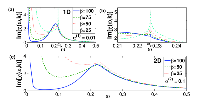
Figure 3: (Color online) The Bragg response (19) at weak polaronic coupling, momentum exchange $k=1$ and for different temperatures ($\beta=\left(k_{B}T\right)^{-1}$) in 1D (a) and 2D (c). In both cases a peak corresponding to the emission of Bogoliubov excitations is observed together with the anomalous Drude peak at $\omega=0$. In 1D another sharp peak is present at $\omega=\omega_{k}$, with $\omega_{k}$ the Bogoliubov dispersion (5). In (b) we have zoomed in on this sharp peak in 1D. All quantities are in polaronic units ($\hbar=m_{I}=\xi=1$).

In figures 5 and 6 we have zoomed in on the tail of the Bogoliubov emission peak for different values of the coupling parameter in 1 and 2 dimensions, respectively. At larger values for the polaronic coupling parameter $\alpha^{\left(d\right)}$ the emergence of a secondary peak is observed. This behavior is also observed in the optical absorption of the Fröhlich solid state polaron where the secondary peak corresponds to a transition to the Relaxed Excited State accompanied by the emission of phonons PhysRevLett.22.94 . The Relaxed Excited State denotes an excitation of the impurity in the relaxed self-induced potential where relaxed means that the self-induced potential is adapted to the excited state wave function of the impurity. In the inset the location of this secondary peak is plotted as a function of the exchanged momentum together with a least square fit to the following quadratically spectrum:

$$\omega\left(k\right)=\omega+\frac{\hbar^{2}k^{2}}{2m},$$ (33)

which shows a good agreement at small $k$. This suggests that the state corresponding to the secondary peak is characterized by a transition frequency $\omega$ and an effective mass $m$ (this was also observed for the 3-dimensional case in Ref. PhysRevA.83.033631 ).

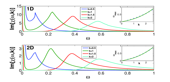
Figure 4: (Color online) The Bragg response at weak polaronic coupling ($\alpha^{\left(d\right)}=0.1$) for different exchanged momenta $k$ in 1 and 2 dimensions and at a temperature $\beta=100$. The inset shows the location of the maximum of the peak as a function of the exchanged momentum (markers) together with a least square fit to the Bogoliubov spectrum (5) (full line), this results in $m_{B}=4.3159$ ($4.2216$) for the fitting parameter in 1D (2D). Everything is in polaronic units ($\hbar=m_{I}=\xi=1$).

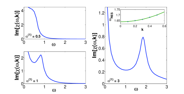
Figure 5: (Color online) Here we zoomed in on the tail of the Bogoliubov emission peak for momentum exchange $k=1$ and temperature $\beta=100$ in 1 dimension. It is clear that at larger values for $\alpha^{\left(1\right)}$ a secondary peak emerges. The inset shows the location of the maximum of this secondary peak at $\alpha^{\left(1\right)}=3$ as a function of the exchanged momentum (markers) together with a least square fit to a quadratic spectrum (33) (solid line), this results in $\omega=1.6386$ and $m=2.0107$ for the fitting parameters. Everything is in polaronic units ($\hbar=m_{I}=\xi=1$).

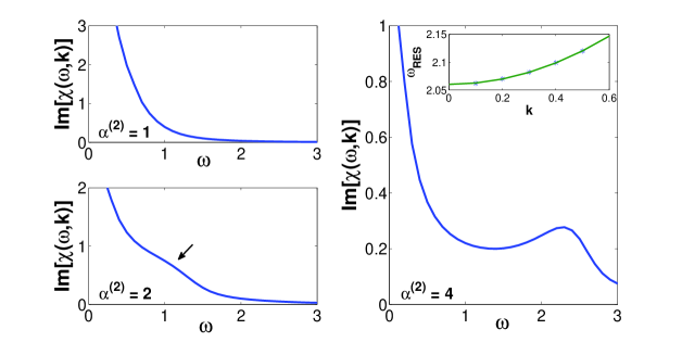
Figure 6: (Color online) Here we zoomed in on the tail of the Bogoliubov emission peak for momentum exchange $k=1$ and temperature $\beta=100$ in 2 dimensions. As in the one-dimensional case a secondary peak emerges at larger values for $\alpha^{\left(2\right)}$. The inset shows the location of the maximum of this secondary peak at $\alpha^{\left(2\right)}=4$ as a function of the exchanged momentum (markers) together with a least square fit to a quadratic spectrum (33) (solid line), this results in $\omega=2.0601$ and $m=2.0755$ for the fitting parameters. Everything is in polaronic units ($\hbar=m_{I}=\xi=1$).

Finally we have checked whether the spectra satisfy the sum rule (23). We calculated the sum of the two terms on the left hand side of expression (23) which is presented in table 1 for $d=1$ and in table 2 for $d=2$ at $\beta=100$ and at different values for $\alpha$ and $k$. These values should be compared to $\pi/2=1.5708$ which results in a fair agreement with small deviations which are to be expected since numerically we had to introduce a cutoff for the $\omega$-integral in (23) and the choice of the parameter $\varepsilon$ in (23) is somewhat arbitrary resulting in a double counting of part of the weight of the Drude peak.

$\alpha^{\left(1\right)}=0.1$ $\alpha^{\left(1\right)}=3$ $k=1$ $1.5440$ $1.5547$ $k=3$ $1.5544$ $1.5743$

Table 1: Here we show the sum of the two terms at the left hand side of the f-sum rule (23) in 1 dimension at $\beta=100$ and at different values for $\alpha^{(1)}$ and $k$.

$\alpha^{\left(2\right)}=1$ $\alpha^{\left(2\right)}=4$ $k=1$ $1.5678$ $1.5734$ $k=3$ $1.5669$ $1.5800$

Table 2: Here we show the sum of the two terms at the left hand side of the f-sum rule (23) in 2 dimensions at $\beta=100$ and at different values for $\alpha^{(2)}$ and $k$.

V Discussion and conclusions

We have applied the calculations for the polaronic ground state properties of an impurity in a Bose-Einstein condensate and the response of this system to Bragg spectroscopy to reduced dimensions. For this purpose we introduced a polaronic coupling parameter $\alpha^{\left(d\right)}$ (15) which depends on the dimension. For growing $\alpha^{\left(d\right)}$ the ground state properties suggest that the self-induced potential accomodates a bound state. As compared to the three-dimensional case the transition to the self-trapped state is much smoother in reduced dimension and for $d=1$ the characteristics of the weak coupling regime are absent.

The Bragg response of the system revealed a peak corresponding to the emission of Bogoliubov excitations, the Drude peak and the emergence of a secondary peak in the strong coupling regime. The amplitude of these polaronic features grows when we go to reduced dimensions. This is important since this indicates that going to reduced dimensions can facilitate an experimental detection of polaronic features. In 1D another sharp peak is observed at weak polaronic coupling that corresponds to the full transition of the exchanged energy and momentum to a Bogoliubov excitation.

Another advantage of considering reduced dimensions is the possibility of using confinement-induced resonances which permits a tuning of the polaronic coupling parameter. These results show that considering an impurity in a Bose-Einstein condensate in reduced dimensions is a very promising candidate to experimentally probe the polaronic strong coupling regime for the first time.

Appendix A Other representation for the self energy

Here we rewrite the self energy (20) to a form which is more suited for numerical calculations. The presented derivation is based on the approach for the optical absorption of the Fröhlich solid state polaron as proposed in Refs. PhysRevB.5.2367 ; PhysRevB.28.6051 . We start by rewriting $D\left(t\right)$ (22) as:

$$D\left(t\right) =\frac{t^{2}}{2\beta\left(m+M\right)}-i\frac{\hbar}{2\left(m+M\right)}t$$

$$+\frac{\hbar M}{2m\Omega\left(m+M\right)}\left\{\coth\left(\frac{\hbar\beta\Omega}{2}\right)-\left[1+n\left(\Omega\right)\right]e^{i\Omega t}-n\left(\Omega\right)e^{-i\Omega t}\right\},$$ (34)

which allows us to write:

$$e^{-k^{2}D\left(t\right)}=e^{-a^{2}\left(\beta\right)k^{2}}\sum_{n,n^{\prime}}k^{2\left(n+n^{\prime}\right)}B\left(\beta,n,n^{\prime}\right)e^{-\frac{k^{2}t^{2}}{2\beta\left(m+M\right)}+it\left[\frac{k^{2}\hbar}{2\left(m+M\right)}+\Omega\left(n-n^{\prime}\right)\right]},$$ (35)

with:

$$a^{2}\left(\beta\right) =\frac{\hbar M}{2m\Omega\left(m+M\right)}\coth\left(\frac{\hbar\beta\Omega}{2}\right);$$

$$B\left(\beta,n,n^{\prime}\right) =\frac{1}{n!}\frac{1}{n^{\prime}!}\left\{a^{2}\left[1+n\left(\Omega\right)\right]\right\}^{n}\left[a^{2}n\left(\Omega\right)\right]^{n^{\prime}};$$ (36)

and $a=a\left(\infty\right)$. If we now use (35) in the expression for the self energy (20) we get:

$$\Sigma\left(\omega,\vec{k}\right) =\frac{2}{m_{I}N\hbar}\sum_{n,n^{\prime}=0}^{\infty}\sum_{\vec{q}\neq 0}\left|V_{\vec{q}}\right|^{2}\frac{\left(\vec{k}.\vec{q}\right)^{2}}{k^{2}}\left|\vec{k}+\vec{q}\right|^{2\left(n+n^{\prime}\right)}B\left(\beta,n,n^{\prime}\right)e^{-a^{2}\left(\beta\right)\left(\vec{k}+\vec{q}\right)^{2}}$$

$$\times\int_{0}^{\infty}dt\left(1-e^{i\omega t}\right)\operatorname{Im}\left\{\left[1+n\left(\omega_{\vec{q}}\right)\right]e^{-\frac{\left(\vec{k}+\vec{q}\right)^{2}}{2\beta\left(m+M\right)}t^{2}+iA^{+}t}+n\left(\omega_{\vec{q}}\right)e^{-\frac{\left(\vec{k}+\vec{q}\right)^{2}}{2\beta\left(m+M\right)}t^{2}+iA^{-}t}\right\},$$ (37)

with:

$$A^{\pm}=\pm\omega_{\vec{q}}+\frac{\left(\vec{k}+\vec{q}\right)^{2}\hbar}{2\left(m+M\right)}+\Omega\left(n-n^{\prime}\right).$$ (38)

We now split the self energy in an imaginary and a real part. Taking the imaginary part of (37) results in:

$$\operatorname{Im}\left[\Sigma\left(\omega,\vec{k}\right)\right] =-\frac{2}{m_{I}N\hbar}\sum_{n,n^{\prime}=0}^{\infty}\sum_{\vec{q}\neq 0}\left|V_{\vec{q}}\right|^{2}\frac{\left(\vec{k}.\vec{q}\right)^{2}}{k^{2}}\left(\vec{k}+\vec{q}\right)^{2\left(n+n^{\prime}\right)}B\left(\beta,n,n^{\prime}\right)e^{-a^{2}\left(\beta\right)\left(\vec{k}+\vec{q}\right)^{2}}$$

$$\times\operatorname{Im}\left(\int_{0}^{\infty}dt\sin\left(\omega t\right)\left\{\left[1+n\left(\omega_{\vec{q}}\right)\right]e^{-\frac{\left(\vec{k}+\vec{q}\right)^{2}}{2\beta\left(m+M\right)}t^{2}+iA^{+}t}\right.\right.$$

$$\left.\left.+n\left(\omega_{\vec{q}}\right)e^{-\frac{\left(\vec{k}+\vec{q}\right)^{2}}{2\beta\left(m+M\right)}t^{2}+iA^{-}t}\right\}\right).$$ (39)

The time integration can now be done (with $C^{2}=\frac{\left(\vec{k}+\vec{q}\right)^{2}}{2\beta\left(m+M\right)}$):

$$\int_{0}^{\infty}dt\sin\left(\omega t\right)\left\{\left[1+n\left(\omega_{\vec{q}}\right)\right]e^{-C^{2}t^{2}+iA^{+}t}+n\left(\omega_{\vec{q}}\right)e^{-C^{2}t^{2}+iA^{-}t}\right\}$$

$$=\frac{1}{2iC}\left\{\left[1+n\left(\omega_{\vec{q}}\right)\right]\left[\frac{\sqrt{\pi}}{2}e^{-\frac{\left(A^{+}+\omega\right)^{2}}{4C^{2}}}+iF\left(\frac{A^{+}+\omega}{2C}\right)-\frac{\sqrt{\pi}}{2}e^{-\frac{\left(A^{+}-\omega\right)^{2}}{4C^{2}}}-iF\left(\frac{A^{+}-\omega}{2C}\right)\right]\right.$$

$$\left.+n\left(\omega_{\vec{q}}\right)\left[\frac{\sqrt{\pi}}{2}e^{-\frac{\left(A^{-}+\omega\right)^{2}}{4C^{2}}}+iF\left(\frac{A^{-}+\omega}{2C}\right)-\frac{\sqrt{\pi}}{2}e^{-\frac{\left(A^{-}-\omega\right)^{2}}{4C^{2}}}-iF\left(\frac{A^{-}-\omega}{2C}\right)\right]\right\}.$$ (40)

Where we introduced the Dawson integral $F\left(x\right)$:

$$F\left(x\right) =e^{-x^{2}}\int_{0}^{x}e^{y^{2}}dy$$

$$=\frac{1}{2}\sqrt{\pi}e^{-x^{2}}\text{erfi}\left(x\right),$$ (41)

where erfi$\left(x\right)$ is the imaginary error function: erfi$\left(x\right)=-i\operatorname{erf}\left(ix\right)$, with $\operatorname{erf}\left(x\right)$ the error function. This finally results in the following expression for the imaginary part of the self energy:

$$\operatorname{Im}\left[\Sigma\left(\omega,\vec{k}\right)\right] =\frac{\sqrt{2\pi\beta\left(m+M\right)}}{2m_{I}N\hbar}\sum_{n,n^{\prime}=0}^{\infty}\sum_{\vec{q}\neq 0}\left|V_{\vec{q}}\right|^{2}\frac{\left(\vec{k}.\vec{q}\right)^{2}}{k^{2}}\left(\vec{k}+\vec{q}\right)^{2\left(n+n^{\prime}\right)-1}B\left(\beta,n,n^{\prime}\right)$$

$$\times e^{-a^{2}\left(\beta\right)\left(\vec{k}+\vec{q}\right)^{2}}\left\{\left[1+n\left(\omega_{\vec{q}}\right)\right]\left[e^{-\frac{\beta\left(m+M\right)\left(A^{+}+\omega\right)^{2}}{2\left(\vec{k}+\vec{q}\right)^{2}}}-e^{-\frac{\beta\left(m+M\right)\left(A^{+}-\omega\right)^{2}}{2\left(\vec{k}+\vec{q}\right)^{2}}}\right]\right.$$

$$\left.+n\left(\omega_{\vec{q}}\right)\left[e^{-\frac{\beta\left(m+M\right)\left(A^{-}+\omega\right)^{2}}{2\left(\vec{k}+\vec{q}\right)^{2}}}-e^{-\frac{\beta\left(m+M\right)\left(A^{-}-\omega\right)^{2}}{2\left(\vec{k}+\vec{q}\right)^{2}}}\right]\right\}.$$ (42)

For the real part of (37) we have:

$$\operatorname{Re}\left[\Sigma\left(\omega,\vec{k}\right)\right] =\frac{2}{m_{I}N\hbar}\sum_{n,n^{\prime}=0}^{\infty}\sum_{\vec{q}\neq 0}\left|V_{\vec{q}}\right|^{2}\frac{\left(\vec{k}.\vec{q}\right)^{2}}{k^{2}}\left(\vec{k}+\vec{q}\right)^{2\left(n+n^{\prime}\right)}B\left(\beta,n,n^{\prime}\right)e^{-a^{2}\left(\beta\right)\left(\vec{k}+\vec{q}\right)^{2}}$$

$$\times\operatorname{Im}\left(\int_{0}^{\infty}dt\left[1-\cos\left(\omega t\right)\right]\left\{\left[1+n\left(\omega_{\vec{q}}\right)\right]e^{-\frac{\left(\vec{k}+\vec{q}\right)^{2}}{2\beta\left(m+M\right)}t^{2}+iA^{+}t}\right.\right.$$

$$\left.\left.+n\left(\omega_{\vec{q}}\right)e^{-\frac{\left(\vec{k}+\vec{q}\right)^{2}}{2\beta\left(m+M\right)}t^{2}+iA^{-}t}\right\}\right).$$ (43)

The time-integration is in this case:

$$\int_{0}^{\infty}dt\left[1-\cos\left(\omega t\right)\right]\left\{\left[1+n\left(\omega_{\vec{q}}\right)\right]e^{-C^{2}t^{2}+iA^{+}t}+n\left(\omega_{\vec{q}}\right)e^{-C^{2}t^{2}+iA^{-}t}\right\}$$

$$=\frac{1}{2C}\left\{\left[1+n\left(\omega_{\vec{q}}\right)\right]\left[\sqrt{\pi}e^{-\frac{\left(A^{+}\right)^{2}}{4C^{2}}}+2iF\left(\frac{A^{+}+\omega}{2C}\right)-\frac{\sqrt{\pi}}{2}e^{-\frac{\left(A^{+}+\omega\right)^{2}}{4C^{2}}}-iF\left(\frac{A^{+}+\omega}{2C}\right)\right.\right.$$

$$\left.-\frac{\sqrt{\pi}}{2}e^{-\frac{\left(A^{+}+\omega\right)^{2}}{4C^{2}}}-iF\left(\frac{A^{+}-\omega}{2C}\right)\right]+n\left(\omega_{\vec{q}}\right)\left[\sqrt{\pi}e^{-\frac{\left(A^{-}\right)^{2}}{4C^{2}}}+2iF\left(\frac{A^{-}+\omega}{2C}\right)\right.$$

$$\left.\left.-\frac{\sqrt{\pi}}{2}e^{-\frac{\left(A^{-}+\omega\right)^{2}}{4C^{2}}}-iF\left(\frac{A^{-}+\omega}{2C}\right)-\frac{\sqrt{\pi}}{2}e^{-\frac{\left(A^{-}+\omega\right)^{2}}{4C^{2}}}-iF\left(\frac{A^{-}-\omega}{2C}\right)\right]\right\}.$$ (44)

This results in the following expression for the real part of the self energy:

$$\operatorname{Re}\left[\Sigma\left(\omega,\vec{k}\right)\right] =\frac{\sqrt{2\beta\left(m+M\right)}}{m_{I}N\hbar}\sum_{n,n^{\prime}=0}^{\infty}\sum_{\vec{q}\neq 0}\left|V_{\vec{q}}\right|^{2}\frac{\left(\vec{k}.\vec{q}\right)^{2}}{k^{2}}\left(\vec{k}+\vec{q}\right)^{2\left(n+n^{\prime}\right)-1}B\left(\beta,n,n^{\prime}\right)$$

$$e^{-a^{2}\left(\beta\right)\left(\vec{k}+\vec{q}\right)^{2}}\left(\left(1+n\left(\omega_{\vec{q}}\right)\right)\left\{2F\left[\frac{\sqrt{2\beta\left(m+M\right)}A^{+}}{2\left|\vec{k}+\vec{q}\right|}\right]\right.\right.$$

$$\left.-F\left[\frac{\sqrt{2\beta\left(m+M\right)}\left(A^{+}+\omega\right)}{2\left|\vec{k}+\vec{q}\right|}\right]-F\left[\frac{\sqrt{2\beta\left(m+M\right)}\left(A^{+}-\omega\right)}{2\left|\vec{k}+\vec{q}\right|}\right]\right\}$$

$$+n\left(\omega_{\vec{q}}\right)\left\{2F\left[\frac{\sqrt{2\beta\left(m+M\right)}A^{-}}{2\left|\vec{k}+\vec{q}\right|}\right]-F\left[\frac{\sqrt{2\beta\left(m+M\right)}\left(A^{-}+\omega\right)}{2\left|\vec{k}+\vec{q}\right|}\right]\right.$$

$$\left.\left.-F\left[\frac{\sqrt{2\beta\left(m+M\right)}\left(A^{-}-\omega\right)}{2\left|\vec{k}+\vec{q}\right|}\right]\right\}\right).$$ (45)

References

• (1) I. Bloch, J. Dalibard, and W. Zwerger, Rev. Mod. Phys. 80, 885 (2008).
• (2) J. T. Devreese and A. S. Alexandrov, Advances In Polaron Physics, volume 159, Springer-Verlag Berlin, 2010.
• (3) F. M. Cucchietti and E. Timmermans, Phys. Rev. Lett. 96, 210401 (2006).
• (4) K. Sacha and E. Timmermans, Phys. Rev. A 73, 063604 (2006).
• (5) M. Bruderer, A. Klein, S. R. Clark, and D. Jaksch, Phys. Rev. A 76, 011605 (2007).
• (6) M. Bruderer, A. Klein, S. R. Clark, and D. Jaksch, New Journal of Physics 10, 033015 (2008).
• (7) M. Bruderer, W. Bao, and D. Jaksch, EPL (Europhysics Letters) 82, 30004 (2008).
• (8) A. Privitera and W. Hofstetter, Phys. Rev. A 82, 063614 (2010).
• (9) D. H. Santamore and E. Timmermans, New Journal of Physics 13, 103029 (2011).
• (10) J. Tempere, W. Casteels, M. K. Oberthaler, S. Knoop, E. Timmermans, and J. T. Devreese, Phys. Rev. B 80, 184504 (2009).
• (11) W. Casteels, T. Van Cauteren, J. Tempere, and J. Devreese, Laser Physics 21, 1480 (2011).
• (12) W. Casteels, J. Tempere, and J. T. Devreese, Phys. Rev. A 84, 063612 (2011).
• (13) W. Casteels, J. Tempere, and J. T. Devreese, Phys. Rev. A 83, 033631 (2011).
• (14) W. Casteels, J. Tempere, and J. Devreese, Journal of Low Temperature Physics 162, 266 (2011).
• (15) N. Spethmann, F. Kindermann, S. John, C. Weber, D. Meschede, and A. Widera, Applied Physics B: Lasers and Optics 106, 1 (2012).
• (16) S. Schmid, A. Härter, and J. H. Denschlag, Phys. Rev. Lett. 105, 133202 (2010).
• (17) J. Catani, L. De Sarlo, G. Barontini, F. Minardi, and M. Inguscio, Phys. Rev. A 77, 011603 (2008).
• (18) B. Gadway, D. Pertot, R. Reimann, and D. Schneble, Phys. Rev. Lett. 105, 045303 (2010).
• (19) J. Catani, G. Lamporesi, D. Naik, M. Gring, M. Inguscio, F. Minardi, A. Kantian, and T. Giamarchi, ArXiv: 1106.0828 (2011).
• (20) R. P. Feynman, Phys. Rev. 97, 660 (1955).
• (21) R. P. Feynman, R. W. Hellwarth, C. K. Iddings, and P. M. Platzman, Phys. Rev. 127, 1004 (1962).
• (22) J. Devreese, J. De Sitter, and M. Goovaerts, Phys. Rev. B 5, 2367 (1972).
• (23) A. S. Mishchenko, N. Nagaosa, N. V. Prokof’ev, A. Sakamoto, and B. V. Svistunov, Phys. Rev. Lett. 91, 236401 (2003).
• (24) G. De Filippis, V. Cataudella, A. S. Mishchenko, C. A. Perroni, and J. T. Devreese, Phys. Rev. Lett. 96, 136405 (2006).
• (25) F. C. Brown, in Polarons and Excitons, Plenum Press, New York, 1963, edited by C. G. Kuper and G. D. Whitfield, p. 323-355.
• (26) J. W. Hodby, G. P. Russell, F. M. Peeters, J. T. Devreese, and D. M. Larsen, Phys. Rev. Lett. 58, 1471 (1987).
• (27) A. S. Alexandrov, Theory of Superconductivity: From Weak to Strong Coupling, IOP publishing, 2003.
• (28) A. S. Alexandrov, Phys. Rev. B 77, 094502 (2008).
• (29) T. Schuster, R. Scelle, A. Trautmann, S. Knoop, M. K. Oberthaler, M. M. Haverhals, M. R. Goosen, S. J. J. M. F. Kokkelmans, and E. Tiemann, Phys. Rev. A 85, 042721 (2012).
• (30) T. Takekoshi, M. Debatin, R. Rameshan, F. Ferlaino, R. Grimm, H.-C. Nägerl, C. R. Le Sueur, J. M. Hutson, P. S. Julienne, S. Kotochigova, and E. Tiemann, Phys. Rev. A 85, 032506 (2012).
• (31) J. W. Park, C.-H. Wu, I. Santiago, T. G. Tiecke, S. Will, P. Ahmadi, and M. W. Zwierlein, Phys. Rev. A 85, 051602 (2012).
• (32) J. Steinhauer, R. Ozeri, N. Katz, and N. Davidson, Phys. Rev. Lett. 88, 120407 (2002).
• (33) D. M. Stamper-Kurn, A. P. Chikkatur, A. Görlitz, S. Inouye, S. Gupta, D. E. Pritchard, and W. Ketterle, Phys. Rev. Lett. 83, 2876 (1999).
• (34) L. Pitaevskii and S. Stringari, Bose-Einstein Condensation, Oxford University Press, first edition, 2003.
• (35) I. Bloch, Nature Physics 1, 23 (2005).
• (36) Y. Nishida and S. Tan, Phys. Rev. Lett. 101, 170401 (2008).
• (37) V. Peano, M. Thorwart, C. Mora, and R. Egger, New Journal of Physics 7, 192 (2005).
• (38) T. Bergeman, M. G. Moore, and M. Olshanii, Phys. Rev. Lett. 91, 163201 (2003).
• (39) M. Olshanii, Phys. Rev. Lett. 81, 938 (1998).
• (40) D. S. Petrov and G. V. Shlyapnikov, Phys. Rev. A 64, 012706 (2001).
• (41) E. Haller, M. J. Mark, R. Hart, J. G. Danzl, L. Reichsöllner, V. Melezhik, P. Schmelcher, and H.-C. Nägerl, Phys. Rev. Lett. 104, 153203 (2010).
• (42) H. Moritz, T. Stöferle, K. Günter, M. Köhl, and T. Esslinger, Phys. Rev. Lett. 94, 210401 (2005).
• (43) E. Haller, M. Gustavsson, M. J. Mark, J. G. Danzl, R. Hart, G. Pupillo, and H.-C. Nägerl, Science 325, 1224 (2009).
• (44) G. Lamporesi, J. Catani, G. Barontini, Y. Nishida, M. Inguscio, and F. Minardi, Phys. Rev. Lett. 104, 153202 (2010).
• (45) B. Fröhlich, M. Feld, E. Vogt, M. Koschorreck, W. Zwerger, and M. Köhl, Phys. Rev. Lett. 106, 105301 (2011).
• (46) F. M. Peeters, W. Xiaoguang, and J. T. Devreese, Phys. Rev. B 33, 3926 (1986).
• (47) W. Xiaoguang, F. M. Peeters, and J. T. Devreese, Phys. Rev. B 31, 3420 (1985).
• (48) F. M. Peeters and J. T. Devreese, Phys. Rev. B 36, 4442 (1987).
• (49) D. S. Petrov, G. V. Shlyapnikov, and J. T. M. Walraven, Phys. Rev. Lett. 85, 3745 (2000).
• (50) D. S. Petrov, M. Holzmann, and G. V. Shlyapnikov, Phys. Rev. Lett. 84, 2551 (2000).
• (51) T. Best, S. Will, U. Schneider, L. Hackermüller, D. van Oosten, I. Bloch, and D.-S. Lühmann, Phys. Rev. Lett. 102, 030408 (2009).
• (52) J. T. Devreese, ArXiv: 1012.4576 (2010).
• (53) R. P. Feynman, Statistical Mechanics: A Set Of Lectures, Addison-Wesley Publ. Co., 1990.
• (54) F. M. Peeters and J. T. Devreese, Phys. Rev. B 31, 4890 (1985).
• (55) D. K. K. Lee and J. M. F. Gunn, Phys. Rev. B 46, 301 (1992).
• (56) J. T. Devreese, L. F. Lemmens, and J. Van Royen, Phys. Rev. B 15, 1212 (1977).
• (57) J. T. Devreese, S. N. Klimin, J. L. M. van Mechelen, and D. van der Marel, Phys. Rev. B 81, 125119 (2010).
• (58) J. L. M. van Mechelen, D. van der Marel, C. Grimaldi, A. B. Kuzmenko, N. P. Armitage, N. Reyren, H. Hagemann, and I. I. Mazin, Phys. Rev. Lett. 100, 226403 (2008).
• (59) V. Gurevich, I. Lang, and Y. Firsov, Sov. Phys. Solid State 4, 918 (1962).
• (60) W. Huybrechts, J. D. Sitter, and J. Devreese, Solid State Communications 13, 163 (1973).
• (61) J. Tempere and J. Devreese, The European Physical Journal B - Condensed Matter and Complex Systems 20, 27 (2001), 10.1007/PL00011092.
• (62) G. D. Mahan, Many-Particle Physics, Plenum, New York, N.Y., 2nd edition, 1993.
• (63) E. Kartheuser, R. Evrard, and J. Devreese, Phys. Rev. Lett. 22, 94 (1969).
• (64) F. M. Peeters and J. T. Devreese, Phys. Rev. B 28, 6051 (1983).