Generalized Wannier functions: a comparison of molecular electric dipole polarizabilities

Abstract

Localized Wannier functions provide an efficient and intuitive means by which to compute dielectric properties from first principles. They are most commonly constructed in a post-processing step, following total-energy minimization. Nonorthogonal generalized Wannier functions (NGWFs) Skylaris et al. (2002); *onetep1 may also be optimized in situ, in the process of solving for the ground-state density. We explore the relationship between NGWFs and orthonormal, maximally localized Wannier functions (MLWFs) Marzari and Vanderbilt (1997); *PhysRevB.65.035109, demonstrating that NGWFs may be used to compute electric dipole polarizabilities efficiently, with no necessity for post-processing optimization, and with an accuracy comparable to MLWFs.

In this Brief Report, we explore the equivalence between nonorthogonal generalized Wannier functions (NGWFs) Skylaris et al. (2002); *onetep1, generated using linear-scaling Kohn-Sham density functional theory (DFT) Hohenberg and Kohn (1964); *PhysRev.140.A1133, and their orthonormal counterparts, particularly maximally localized Wannier functions (MLWFs) Marzari and Vanderbilt (1997); *PhysRevB.65.035109, both recently reviewed in Ref. Marzari et al., 2012. We demonstrate the comparable, high accuracy of the two formalisms for dielectric response, laying the foundation for large-scale calculation of optical properties.

We begin with the single-particle density-matrix defined, for a given set of Bloch orbitals $\lvert\psi_{n\mathbf{k}}\rangle$, where $n$ indexes occupied bands, $\mathbf{k}$ is the crystal wave-vector and we suppress the spin index for notational clarity, by

$$\hat{\rho}=\sum_{n}\int_{1\rm{BZ}}d\mathbf{k}\;\lvert\psi_{n\mathbf{k}}\rangle f_{n\mathbf{k}}\langle\psi_{n\mathbf{k}}\rvert.$$ (1)

Here, $1\rm{BZ}$ is the first Brillouin zone corresponding to the periodic unit cell of volume $V_{\rm cell}$. A reformulation of such Bloch states suitable for the study of spatially localized properties was proposed by Wannier Wannier (1937), whose eponymously named functions are defined, for a unit cell at the lattice vector $\mathbf{R}$, by

$$\lvert w_{n\mathbf{R}}\rangle=\sqrt{\frac{V_{\rm cell}}{\left(2\pi\right)^{3}}}\int_{1\rm{BZ}}d\mathbf{k}\;e^{-i\mathbf{k}\cdot\mathbf{R}}\lvert\psi_{n\mathbf{k}}\rangle.$$ (2)

The orthonormality of Bloch orbitals is preserved,

$$\langle w_{n\mathbf{R}}\rvert w_{m\mathbf{R^{\prime}}}\rangle=\delta_{nm}\delta_{\mathbf{R}\mathbf{R^{\prime}}},$$ (3)

and we may choose the gauge freely, so that any prior unitary transformation among the orbitals, $\lvert\tilde{\psi}_{n\mathbf{k}}\rangle=\sum_{m}\lvert\psi_{m\mathbf{k}}\rangle U_{mn\mathbf{k}}$, may also give rise to a valid set of generalized Wannier functions, via Eq. 2. Unoccupied states may be included in the wannierization, while maintaining the same occupied density, by appropriately transforming the occupancy of the orbitals to give $f_{n\mathbf{k}}$, to give $\tilde{f}_{nm\mathbf{k}}=\sum_{p}U^{\dagger}_{np\mathbf{k}}f_{p\mathbf{k}}U_{pm\mathbf{k}}$. The density-matrix may be readily expressed in terms of Wannier functions, in the separable form proposed in Ref. McWeeny, 1960, and given by

$$\hat{\rho} {}=\sum_{\mathbf{R}\mathbf{R^{\prime}}}\lvert w_{n\mathbf{R}}\rangle k_{nm\mathbf{R^{\prime}}-\mathbf{R}}\langle w_{m\mathbf{R^{\prime}}}\rvert,\quad\mbox{where}$$ (4a)

$$k_{nm\mathbf{R}} {}=\frac{V_{\rm cell}}{\left(2\pi\right)^{3}}\int_{1\rm{BZ}}d\mathbf{k}\;e^{-i\mathbf{k}\cdot\mathbf{R}}\tilde{f}_{nm\mathbf{k}},$$ (4b)

is commonly known as the density kernel.

The extension of this formalism to nonorthogonal generalized Wannier functions (NGWFs) is both of practical interest and utility. Orthonormality and spatial localization are generally competing requirements Anderson (1968), hence nonorthogonal orbitals may form a more efficient basis in which to expand short-ranged operators and, as a result, they are used extensively in linear-scaling DFT approaches. We may express these NGWFs, $\lvert\phi_{\alpha\mathbf{R}}\rangle$, simply in terms of the generalization of the transformation matrices $U_{\mathbf{k}}$ to possible non-unitarity matrices $M_{\mathbf{k}}$, that is $M_{n\alpha\mathbf{k}}=\langle\psi_{n\mathbf{k}}\rvert\tilde{\psi}_{\alpha\mathbf{k}}\rangle$, whereafter $\tilde{f}_{\alpha\beta\mathbf{k}}=\sum_{n}M^{\dagger}_{\alpha n\mathbf{k}}f_{n\mathbf{k}}M_{n\beta\mathbf{k}}$. We use Latin and Greek letters to index orthonormal and nonorthogonal sets, respectively, and implicitly sum over repeated index pairs.

In the nonorthogonal case, the density-matrix may be expanded in separable form via the tensor contraction

$$\hat{\rho} {}=\sum_{\mathbf{R}\mathbf{R^{\prime}}}\lvert\phi_{\alpha\mathbf{R}}\rangle K^{\alpha\beta}_{\mathbf{R^{\prime}}-\mathbf{R}}\langle\phi_{\beta\mathbf{R^{\prime}}}\rvert,\quad\mbox{where}$$ (5a)

$$K^{\alpha\beta}_{\mathbf{R}} {}=\frac{V_{\rm cell}}{\left(2\pi\right)^{3}}\int_{1\rm{BZ}}d\mathbf{k}\;e^{-i\mathbf{k}\cdot\mathbf{R}}S^{\alpha\gamma}\tilde{f}_{\gamma\delta\mathbf{k}}S^{\delta\beta},$$ (5b)

and the price to be paid for nonorthogonality is a nontrivial metric tensor given by $S_{\alpha\beta}=\langle\phi_{\alpha\mathbf{R}}\rvert\phi_{\beta\mathbf{R^{\prime}}}\rangle\delta_{\mathbf{R}\mathbf{R^{\prime}}}$, which defines the inter-relationship between covariant vectors, $\lvert\phi_{\alpha\mathbf{R}}\rangle=\lvert\phi^{\beta}_{\mathbf{R}}\rangle S_{\beta\alpha}$, and contravariant vectors (NGWF duals) $\lvert\phi^{\alpha}_{\mathbf{R}}\rangle=\lvert\phi_{\beta\mathbf{R}}\rangle S^{\beta\alpha}$. The contravariant metric $S^{\alpha\beta}$ in Eq. 5b is defined such that $S_{\alpha\gamma}S^{\gamma\beta}\equiv\delta_{\alpha}^{\;\;\beta}$, and is also independent of the lattice vector. Orthonormality is thus replaced by the general tensor expression

$$\langle\phi_{\alpha\mathbf{R}}\rvert\phi_{\gamma\mathbf{R^{\prime}}}\rangle S^{\gamma\beta}=S_{\alpha\gamma}\langle\phi^{\gamma}_{\mathbf{R}}\rvert\phi^{\beta}_{\mathbf{R^{\prime}}}\rangle=\delta_{\alpha}^{\;\;\beta}\delta_{\mathbf{R}\mathbf{R^{\prime}}}.$$ (6)

Numerous optimization procedures have been developed for ab initio Wannier functions. A widespread approach involves their construction in a post-processing step, computing the $U_{nm\mathbf{k}}$ or $M_{n\alpha\mathbf{k}}$ matrices, and then the generalized occupancies $\tilde{f}_{\mathbf{k}}$, following the computation of the delocalized orbitals. However, it has been recognized, and utilized in the context of large-scale calculations for some time Hernández and Gillan (1995); *0953-8984-14-11-303; *PhysRevB.47.9973; *PhysRevB.50.4316; *PhysRevB.51.1456; *PhysRevB.67.155108; *liu:1634, that localized Wannier functions may also be optimized directly in situ, that is during the process of solving for the electronic structure. In the latter, the basis expansion of the functions, $\left\{\phi_{\alpha\mathbf{R}}\left(\mathbf{r}\right)\right\}$ and the corresponding density kernel $K_{\mathbf{R}}^{\alpha\beta}$ must be optimized together, reconstructing the delocalized orbitals afterwards only if necessary.

A variety of plausible criteria may also be employed for Wannier function optimization in either case, such as energy downfolding Yamasaki et al. (2006) or maximal Coulomb repulsion Miyake and Aryasetiawan (2008), or, as used in this work, total-energy minimization or spatial localization. Depending on their definition, these criteria may or may not uniquely define the Wannier functions, in that they may admit some residual gauge freedom. A particularly efficacious measure for localization is the second central moment which, for a set of Wannier functions $\left\{\lvert w_{n\mathbf{R}}\rangle\right\}$ takes the form of the spread functional,

$$\Omega {}=\sum_{n}\left[\langle w_{n\mathbf{0}}\rvert r^{2}\lvert w_{n\mathbf{0}}\rangle-\langle w_{n\mathbf{0}}\rvert\mathbf{r}\lvert w_{n\mathbf{0}}\rangle^{2}\right],$$ (7)

where the generalization to the nonorthogonal case does not yield straightforward physical interpretation. MLWFs Marzari and Vanderbilt (1997); *PhysRevB.65.035109 are those orthonormal Wannier functions generated by unitary transformations $U_{nm\mathbf{k}}$ that minimize $\Omega$, for a fixed set of orbitals. MLWFs are usually computed in a post-processing procedure, using an implementation such as Wannier90 A. A. Mostofi, J. R. Yates, Y.-S. Lee, I. Souza, D. Vanderbilt and N. Marzari (2008), and have been widely adopted as an accurate minimal basis with which to compute numerous ground-state and excited-state properties, as well as to augment DFT with many-body interactions Marzari et al. (2012). MLWFs have been used to great effect, moreover, in the context of molecular dynamics, particularly interesting examples including the calculation of the dielectric permittivity and dipolar correlation of liquid water Sharma et al. (2007), as well as its dynamical charge and dipole tensors Pasquarello and Resta (2003).

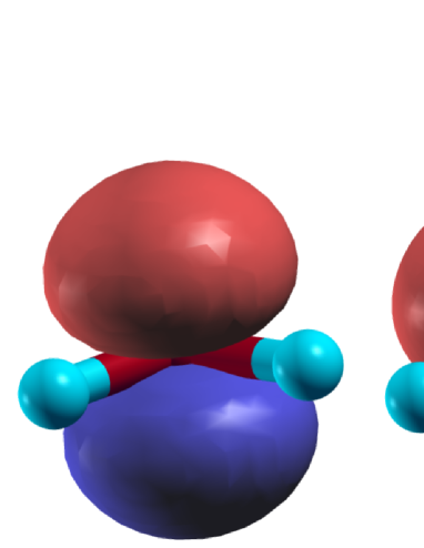
Figure 1: (Color online) Wannier functions, NGWF (left) and MLWF (right), of predominantly oxygen $p_{z^{2}}$ (highest occupied, $1b_{1}$) character in H₂O, at zero applied field, with iso-surfaces at one sixth of their respective maxima. Both types retain some residual arbitrariness following optimization.

NGWFs, unlike their orthonormal counterparts, are more commonly optimized in situ, as a by-product of total-energy minimization with respect to the density-matrix, for example, in the ONETEP linear-scaling DFT code Skylaris et al. (2002); *onetep1; Hine et al. (2009). In the latter, NGWFs are expanded in a fixed underlying basis of periodic cardinal sine functions (also known as psinc A. A. Mostofi, P. D. Haynes, C.-K. Skylaris and M. C. Payne (2003) or band-width limited $\delta$-functions), whose spatial finesse is determined by a single variational parameter, the kinetic energy cutoff of the equivalent plane-wave basis. The NGWFs are then those functions, when traced with their corresponding optimized density kernel, which reproduce the ground-state density-matrix, whence the ground-state energy

$$E_{0} {}=\min_{n}E\left[n\right]=\min_{\hat{\rho}}E\left[\hat{\rho}\right]_{\hat{\rho}=\hat{\rho}^{2}}$$ (8)

$${}=\min_{\mathbf{K},\{\phi\}}E\left[\mathbf{K},\{\phi\}\right]_{\mathbf{K}=\mathbf{K}\mathbf{S}\mathbf{K}}.$$

In practice, in order to extremize the total-energy with respect to idempotent density matrices, two nested conjugate-gradients variational minimization procedures are performed. In the inner loop, the energy is minimized with respect to the elements of the density kernel, for a fixed NGWF expansion, and in the outer, the density kernel is kept fixed while the total energy is minimized with respect to the NGWF psinc-expansion. A number of similar methods have been proposed in which equations of motion generate optimized nonorthogonal functions Hernández and Gillan (1995); *0953-8984-14-11-303; *PhysRevB.47.9973; *PhysRevB.50.4316; *PhysRevB.51.1456; *PhysRevB.67.155108; *liu:1634.

An intuitive interpretation of Wannier functions is furnished via the modern theory of polarization King-Smith and Vanderbilt (1993); *resta, in that changes in their centers $\langle\mathbf{r}\rangle_{nm}=\langle w_{n\mathbf{0}}\rvert\mathbf{r}\lvert w_{m\mathbf{0}}\rangle$ exactly reproduce, and thus may be used to efficiently calculate, changes in the polarization of insulating systems. The change in electronic polarization $\delta\mathbf{P}$, subject to a gap-preserving perturbation, may be expressed as

$$\delta\mathbf{P}{} =-\frac{2e}{V_{\rm cell}}\sum_{n}^{N}\delta\langle\mathbf{r}\rangle_{nn}\;\;\left(\mbox{if}\;\tilde{f}_{nm}=\delta_{nm},n\leq N\right),$$ (9a)

$$=-\frac{2e}{V_{\rm cell}}\left[\delta K_{\mathbf{0}}^{\alpha\beta}\langle\mathbf{r}\rangle_{\beta\alpha}+K_{\mathbf{0}}^{\alpha\beta}\delta\langle\mathbf{r}\rangle_{\beta\alpha}\right],$$ (9b)

where the $\mathbf{k}$-independence of the occupancies (also spin-degenerate) implies that it is sufficient to consider only the $\mathbf{R}=\mathbf{0}$ term. Here, respectively, we have provided the orthonormal case for $N$ occupied bands, and the more general, nonorthogonal case.

It has been shown that close-to-orthonormal Wannier functions generated by means of direct minimization, of an appropriately constructed functional, may be used to efficiently compute dielectric properties Fernández et al. (1997); *PhysRevB.58.R7480. It is of importance, particularly for linear-scaling methods, to generalize this result and verify that in situ optimized NGWFs can reproduce electronic response properties with the same reliability as that of the well documented MLWFs, as NGWFs are increasingly being used in large-scale methods for spectral partitioning and dielectric properties, particularly in molecular systems Ratcliff et al. (2011); *PhysRevB.85.115404; *PhysRevB.82.081102. The simplest such response property is perhaps the high-frequency (termed “clamped-ion” or “static”) linear dipole polarizability tensor

$$\alpha_{ij}=\lim_{\omega\rightarrow\infty}\alpha_{ij}\left(\omega\right)=\left.\frac{\partial P_{i}}{\partial\mathcal{E}_{j}}\right|_{\delta\mathbf{R}_{\rm{ion}}=0},$$ (10)

where $\mathbf{\mathcal{E}}$ is an applied electric field within the dipole approximation. This polarizability is somewhat different from that which is most frequently probed experimentally, namely the static or visual frequency regimes, and neglects the response of the ionic positions.

$\bar{\alpha}$ NGWF MLWF Gaussian Experiment H2O 10.58 10.47 10.76a, 7.4b 9.64d, 9.79f NH3 15.28 15.24 15.63a, 12.1b 14.56d, 18.9e CH4 17.70 17.49 17.74a, 14.8b 17.27d, 17.5e,f C2H4 28.50 28.39 28.77a, 25.6b 27.70d, 28.69f CO 13.64 13.53 13.73a, 12.1b 13.09d, 12.8e, 13.16f CO2 18.00 17.85 18.06a, 14.8b 17.51d, 19.6e,f, 17.48f N2 11.99 11.87 12.31a, 10.8b 11.74d,f, 11.5e C10H8 122.8 123.0 121.76c 117.4x,y, 118.9z $\kappa$ NGWF MLWF Gaussian Experiment H2O 0.16 0.14 0.14a 0.67d NH3 2.45 2.64 2.70a 1.94d C2H4 12.18 12.03 11.94a 11.4d CO 3.53 3.54 3.55a 3.57d CO2 13.88 13.96 13.70a 13.83d, 13.70f N2 4.50 4.55 4.83a 4.59d, 4.45f C10H8 96.1 94.8 94.13c 86.9x, 79.0y, 63.6z

(a) Static polarizability in a d-aug-cpVTZ basis van Caillie and Amos (2000).

(b) Static PBE polarizability in 6-311++G(d,p) basis at

(b) B3LYP/6-311G** optimised geometries Zope et al. (2008).

(c) Static polarizability in Sadlej pVTZ basis Hammond et al. (2007).

(d) Compiled in Ref. van Caillie and Amos, 2000, based on analysis of anisotropy data Olney et al. (1997); *spackman:1288; *spackman2.

(e) CRC Handbook Lide (2006). (f) Extrapolated Rayleigh scattering Alms et al. (1975).

(x) Anisotropic refraction Vuks (1966). (y) Laser Stark spectroscopy Heitz et al. (1992); Vuks (1966).

(z) Optical measurements at $632.8$ nm in solution Calvert and Ritchie (1980).

Table 1: Isotropic ($\bar{\alpha}$) and anisotropic ($\kappa$) polarizabilities (e² a${}_{0}^{2}$ Ha^-1), from DFT using nonorthogonal (NGWF) and orthonormal (MLWF) Wannier functions. Previous Gaussian-basis calculations Perdew et al. (1996), and experimental values are included.

Two different Kohn-Sham DFT packages were used in order to compute polarizabilities within the NGWF and MLWF formalisms, respectively the ONETEP linear-scaling code Skylaris et al. (2002); *onetep1; Hine et al. (2009), and a combination of a plane-wave pseudopotential package QE and the Wannier90 A. A. Mostofi, J. R. Yates, Y.-S. Lee, I. Souza, D. Vanderbilt and N. Marzari (2008) code. An example of each type of function is depicted in Fig.1. A set of well-isolated, closed-shell molecules were selected, so that a sawtooth-potential representation of the electric field could be used, with the potential boundary maximally distant from the molecules, up to a maximum field value of $\pm 8.0\times 10^{-5}$ Ha e^-1 a${}_{0}^{-1}$, in intervals of $2.0\times 10^{-5}$ Ha e^-1 a${}_{0}^{-1}$, for all systems. The response remained well within the linear regime at these field values, which lay well below the threshold for Zener breakdown. The rates of change in polarization was calculated using linear-regression of finite-difference data. Identical norm-conserving pseudopotentials opi were used in both cases, having been generated in the required formats, the Perdew-Burke-Ernzerhof (PBE) exchange-correlation approximation Perdew et al. (1996), and the same run-time parameters and analysis were used for both codes so far as possible. Zero-field ground-state geometries were optimized using ONETEP, in cubic simulation cells of side length $40$ a₀ ($50$ a₀ in the case of naphthalene C₁₀H₈). The density and potential were fully reset to those of atomic superpositions upon each incrementation of the field. An equivalent plane-wave cutoff of $1000$ eV, $\Gamma$-point Brillouin zone sampling, no density-kernel truncation and NGWFs with a $10$ a₀ radius cutoff were used.

In the case of nonaxially symmetric molecules, random initial guesses for the MLWFs were regenerated at each incrementation of the electric field. For axially symmetric molecules such as CO, CO₂ and N₂, however, the maximal localization condition does not uniquely define the MLWF centers under rotations about the axis, as discussed in Ref. Andrinopoulos et al., 2011. While the sum of centers, and hence the transverse response, should be well-defined, in practice this unbroken symmetry results in excessively noisy linear-response data. It was found, however, that re-initializing the MLWFs to $s$-orbitals at each field value, with centers coinciding with a set of zero-field MLWFs, proved sufficiently robust to obtain excellent linear fitting. No such measures were necessary in the case of ONETEP NGWFs, due to an effective symmetry breaking introduced by the underlying real-space psinc grid.

The isotropic and anisotropic parts of the polarizability tensor $\mathbf{\alpha}$ are defined, respectively, as

$$\bar{\alpha}=\frac{1}{3}\rm{tr}\left[\mathbf{\alpha}\right],\quad\kappa=\sqrt{\frac{3}{2}\rm{tr}\left[\mathbf{\alpha}^{2}\right]-\frac{1}{2}\left(\rm{tr}\left[\mathbf{\alpha}\right]\right)^{2}},$$ (11)

our computed values of which using NGWFs and MLWFs are shown in Table 1. The quadratic mean fractional discrepancy between the isotropic parts was $8.0\times 10^{-3}$, while the discrepancy was greater for the anisotropic parts, at $4.1\times 10^{-2}$. As judged by the arithmetic mean fractional discrepancies (given henceforth in parentheses), the NGWFs tended to provide slightly larger isotropic parts (by $6.6\times 10^{-3}$), and also anisotropic parts (by $1.3\times 10^{-3}$), than the MLWFs. Perhaps serendipitously, the NGWF values lay closer than the MLWF results, for the isotropic parts, in all cases, to the previous DFT(PBE) calculations of Ref. van Caillie and Amos, 2000, computed using a sophisticated time-dependent coupled-perturbed method with a triple-$\zeta$ Gaussian basis set; the quadratic (arithmetic) mean discrepancies with respect to these previous results were $1.5\times 10^{-2}$ ($1.3\times 10^{-2}$) and $2.2\times 10^{-2}$ ($2.0\times 10^{-2}$), respectively. The trend was reversed for anisotropies.

Polarizabilities calculated using the related Wannier function varieties agree rather well in spite of the the significant technical dissimilarities between the ab initio packages generating them, and there are a number of possible origins for the small discrepancies observed. First considering the NGWF and MLWF values, both based on the plane-wave formalism and using the same ionic geometry, the NGWF method is the more approximate in that it spatially truncates the Wannier functions and the kinetic-energy operator. Moreover, these methods differ in their handling of pseudopotentials, and, substantially, in their energy-minimization algorithms. With respect to the previous Gaussian-basis results of Ref. van Caillie and Amos, 2000, the possible origins for discrepancy are manifold, most notably, the ionic geometries employed differ and the latter method treats the core electrons explicitly.

The probable errors (arising from the linear fit to the data) in the isotropic and anisotropic polarizabilities, denoted $\Delta\bar{\alpha}$ and $\Delta\kappa$, respectively, and given by

$$\Delta\bar{\alpha} {}=\sqrt{\sum_{ij}\left(\frac{\partial\bar{\alpha}}{\partial\alpha_{ij}}\Delta\alpha_{ij}\right)^{2}}=\frac{1}{3}\sqrt{\sum_{i}\left(\Delta\alpha_{ii}\right)^{2}},$$ (12a)

$$\Delta\kappa {}=\kappa^{-1}\sqrt{\sum_{ij}\left[\left(\frac{3\alpha_{ji}}{2}-\sum_{k}\alpha_{kk}\frac{\delta_{ji}}{2}\right)\Delta\alpha_{ij}\right]^{2}},$$ (12b)

were computed using the unbiased variance estimate $\left(\Delta\alpha_{ij}\right)^{2}$ on each polarizability component $\alpha_{ij}$, and are shown in Table 2. The noise in the data for NGWFs is somewhat more system dependent, as the NGWF truncation depends on the ionic geometry, and higher than in the MLWF case for most of the molecules studied. The quadratic (arithmetic) mean of the ratio of the estimated error in the isotropic polarizability $\bar{\alpha}$ to its value was estimated at $1\times 10^{-3}$ ($4\times 10^{-4}$) for NGWFs and $2\times 10^{-4}$ ($2\times 10^{-4}$) for MLWFs. Correspondingly, for the anisotropic part $\Delta\alpha$, we estimated these ratios to be, respectively, $1\times 10^{-2}$ ($7\times 10^{-3}$) and $3\times 10^{-3}$ ($2\times 10^{-3}$). Nonetheless, the probable errors in the linear fits to the polarizability data were extremely small using both methods, and inconsequential with respect to the expected errors in the approximate functional.

$\Delta\bar{\alpha}/\bar{\alpha}$	NGWF	MLWF	$\Delta\kappa/\kappa$	NGWF	MLWF
H2O	$1\times 10^{-4}$	$8\times 10^{-5}$	NH3	$8\times 10^{-3}$	$8\times 10^{-3}$
NH3	$3\times 10^{-3}$	$5\times 10^{-5}$	NH3	$4\times 10^{-2}$	$5\times 10^{-4}$
CH4	$1\times 10^{-4}$	$5\times 10^{-5}$	CH4	-	-
C2H4	$3\times 10^{-5}$	$3\times 10^{-5}$	C2H4	$2\times 10^{-4}$	$2\times 10^{-4}$
CO	$2\times 10^{-4}$	$3\times 10^{-4}$	CO	$2\times 10^{-3}$	$2\times 10^{-3}$
CO2	$2\times 10^{-5}$	$2\times 10^{-4}$	CO2	$5\times 10^{-5}$	$4\times 10^{-4}$
N2	$6\times 10^{-6}$	$3\times 10^{-4}$	N2	$5\times 10^{-5}$	$2\times 10^{-3}$
C10H8	$4\times 10^{-4}$	$4\times 10^{-4}$	C10H8	$1\times 10^{-3}$	$1\times 10^{-3}$

Table 2: Probable fractional errors in molecular electric polarizabilities computed using NGWFs and MLWFs.

In conclusion, we have shown that nonorthogonal Wannier functions optimized in situ may be used to compute molecular polarizabilities with an accuracy comparable to MLWFs post-processed from plane-wave DFT. This result is promising for the computation of numerous dielectric properties, and the full application of linear-scaling Wannier function analysis to large systems. A promising avenue for future work is the generalization of a method for the dielectric response in extended systems, such as that described in Ref. Nunes and Vanderbilt, 1994 and applied to solids in Ref. Fernández et al., 1997; *PhysRevB.58.R7480, to the linear-scaling NGWF formalism.

We are grateful to John Biggins and Danny Cole for helpful discussions, and to Mark Robinson and Peter Haynes for provision of software. D.D.O’R acknowledges the support of EPSRC and the National University of Ireland. M.C.P. acknowledges EPSRC support (Grants No. EP/G055904/1 and No. EP/F032773/1). A.A.M. acknowledges the support of EPSRC (EP/G05567X/1) and RCUK.

References

- Skylaris et al. (2002) C.-K. Skylaris, A. A. Mostofi, P. D. Haynes, O. Diéguez, and M. C. Payne, Phys. Rev. B, 66, 035119 (2002).
- C.-K. Skylaris, P. D. Haynes, A. A. Mostofi and M. C. Payne (2005) C.-K. Skylaris, P. D. Haynes, A. A. Mostofi and M. C. Payne, J. Chem. Phys., 122, 084119 (2005).
- Marzari and Vanderbilt (1997) N. Marzari and D. Vanderbilt, Phys. Rev. B, 56, 12847 (1997).
- Souza et al. (2001) I. Souza, N. Marzari, and D. Vanderbilt, Phys. Rev. B, 65, 035109 (2001).
- Hohenberg and Kohn (1964) P. Hohenberg and W. Kohn, Phys. Rev., 136, B864 (1964).
- Kohn and Sham (1965) W. Kohn and L. J. Sham, Phys. Rev., 140, A1133 (1965).
- Marzari et al. (2012) N. Marzari, A. A. Mostofi, J. R. Yates, I. Souza, and D. Vanderbilt, (in press, 2012), Rep. Prog. Phys., eprint arXiv:1112.5411 .
- Wannier (1937) G. H. Wannier, Phys. Rev., 52, 191 (1937).
- McWeeny (1960) R. McWeeny, Rev. Mod. Phys., 32, 335 (1960).
- Anderson (1968) P. W. Anderson, Phys. Rev. Lett., 21, 13 (1968).
- Hernández and Gillan (1995) E. Hernández and M. J. Gillan, Phys. Rev. B, 51, 10157 (1995).
- Bowler et al. (2002) D. R. Bowler, T. Miyazaki, and M. J. Gillan, Journal of Physics: Condensed Matter, 14, 2781 (2002).
- Mauri et al. (1993) F. Mauri, G. Galli, and R. Car, Phys. Rev. B, 47, 9973 (1993).
- Mauri and Galli (1994) F. Mauri and G. Galli, Phys. Rev. B, 50, 4316 (1994).
- Ordejón et al. (1995) P. Ordejón, D. A. Drabold, R. M. Martin, and M. P. Grumbach, Phys. Rev. B, 51, 1456 (1995).
- Ozaki (2003) T. Ozaki, Phys. Rev. B, 67, 155108 (2003).
- Liu et al. (2000) S. Liu, J. M. Pérez-Jordá, and W. Yang, J. Chem. Phys., 112, 1634 (2000).
- Yamasaki et al. (2006) A. Yamasaki, M. Feldbacher, Y.-F. Yang, O. K. Andersen, and K. Held, Phys. Rev. Lett., 96, 166401 (2006).
- Miyake and Aryasetiawan (2008) T. Miyake and F. Aryasetiawan, Phys. Rev. B, 77, 085122 (2008).
- A. A. Mostofi, J. R. Yates, Y.-S. Lee, I. Souza, D. Vanderbilt and N. Marzari (2008) A. A. Mostofi, J. R. Yates, Y.-S. Lee, I. Souza, D. Vanderbilt and N. Marzari, Comp. Phys. Comm., 178, 685 (2008).
- Sharma et al. (2007) M. Sharma, R. Resta, and R. Car, Phys. Rev. Lett., 98, 247401 (2007).
- Pasquarello and Resta (2003) A. Pasquarello and R. Resta, Phys. Rev. B, 68, 174302 (2003).
- Hine et al. (2009) N. Hine, P. Haynes, A. Mostofi, C.-K. Skylaris, and M. Payne, Comput. Phys. Commun., 180, 1041 (2009).
- A. A. Mostofi, P. D. Haynes, C.-K. Skylaris and M. C. Payne (2003) A. A. Mostofi, P. D. Haynes, C.-K. Skylaris and M. C. Payne, J. Chem. Phys., 119, 8842 (2003).
- King-Smith and Vanderbilt (1993) R. D. King-Smith and D. Vanderbilt, Phys. Rev. B, 47, 1651 (1993).
- Resta (1994) R. Resta, Rev. Mod. Phys., 66, 899 (1994).
- Fernández et al. (1997) P. Fernández, A. Dal Corso, A. Baldereschi, and F. Mauri, Phys. Rev. B, 55, R1909 (1997).
- Fernández et al. (1998) P. Fernández, A. Dal Corso, and A. Baldereschi, Phys. Rev. B, 58, R7480 (1998).
- Ratcliff et al. (2011) L. E. Ratcliff, N. D. M. Hine, and P. D. Haynes, Phys. Rev. B, 84, 165131 (2011).
- Avraam et al. (2012) P. W. Avraam, N. D. M. Hine, P. Tangney, and P. D. Haynes, Phys. Rev. B, 85, 115404 (2012).
- O’Regan et al. (2010) D. D. O’Regan, N. D. M. Hine, M. C. Payne, and A. A. Mostofi, Phys. Rev. B, 82, 081102 (2010).
- van Caillie and Amos (2000) C. van Caillie and R. D. Amos, Chem. Phys. Lett., 328, 446 (2000).
- Zope et al. (2008) R. R. Zope, T. Baruah, M. R. Pederson, and B. I. Dunlap, Int. J. Quant. Chem., 108, 307 (2008).
- Hammond et al. (2007) J. R. Hammond, K. Kowalski, and W. A. deJong, J. Chem. Phys., 127, 144105 (2007).
- Olney et al. (1997) T. N. Olney, N. M. Cann, G. Cooper, and C. E. Brion, Chemical Physics, 223, 59 (1997).
- Spackman (1991) M. A. Spackman, J. Chem. Phys., 94, 1288 (1991).
- Dougherty and Spackman (1994) J. Dougherty and M. A. Spackman, Molecular Physics, 82, 193 (1994).
- Lide (2006) D. P. Lide, ed., CRC Handbook., 87th ed. (CRC Press/Taylor and Francis Group, Boca Raton, FL., 2006).
- Alms et al. (1975) G. R. Alms, A. Burnham, and W. H. Flygare, J. Chem. Phys., 63, 3321 (1975).
- Vuks (1966) H. F. Vuks, Opt. Spectrosc., 20, 361 (1966).
- Heitz et al. (1992) S. Heitz, D. Weidauer, B. Rosenow, and A. Hese, J. Chem. Phys., 96, 976 (1992).
- Calvert and Ritchie (1980) R. L. Calvert and G. L. D. Ritchie, J. Chem. Soc., Faraday Trans, 2, 1249 (1980).
- Perdew et al. (1996) J. P. Perdew, K. Burke, and M. Ernzerhof, Phys. Rev. Lett., 77, 3865 (1996).
- (44) Quantum Espresso: http://www.quantum-espresso.org.
- (45) Opium pseudopotentials: http://opium.sourceforge.net.
- Andrinopoulos et al. (2011) L. Andrinopoulos, N. D. M. Hine, and A. A. Mostofi, J. Chem. Phys., 135, 154105 (2011).
- Nunes and Vanderbilt (1994) R. W. Nunes and D. Vanderbilt, Phys. Rev. Lett., 73, 712 (1994).