Multiorbital analysis of the effects of uniaxial and hydrostatic pressure on $T_{c}$ in the single-layered cuprate superconductors

Abstract

The origin of uniaxial and hydrostatic pressure effects on $T_{c}$ in the single-layered cuprate superconductors is theoretically explored. A two-orbital model, derived from first principles and analyzed with the fluctuation exchange approximation gives axial-dependent pressure coefficients, $\partial T_{c}/\partial P_{a}>0$, $\partial T_{c}/\partial P_{c}<0$, with a hydrostatic response $\partial T_{c}/\partial P>0$ for both La214 and Hg1201 cuprates, in qualitative agreement with experiments. Physically, this is shown to come from a unified picture in which higher $T_{c}$ is achieved with an “orbital distillation”, namely, the less the $d_{x^{2}-y^{2}}$ main band is hybridized with the $d_{z^{2}}$ and $4s$ orbitals higher the $T_{c}$. Some implications for obtaining higher $T_{c}$ materials are discussed.

I INTRODUCTION

In the physics of high-$T_{c}$ cuprates, optimizing their $T_{c}$ remains a fundamental yet still open problem. Empirically, important parameters that control $T_{c}$ have been identified for the cuprates, i.e., chemical composition, structural parameters, the number of layers, etc, besides the doping concentration. For the structural parameters specifically, several key quantities have been suggested: the bond length between copper and in-plane oxygen($l$, defined in Fig.1)Jorgensen ; Bianconi , and the Cu-apical oxygen distance ($h_{\rm O}$) Maekawa ; Andersen ; Feiner ; Pavarini ; Kotliar ; Weber ; Takimoto ; PRL ; PRB .

Now, the pressure effect is exceptionally valuable as an in situ way to probe the structure-dependence of $T_{c}$. Regarding this, two general observations have been made for the cuprates: (i) $T_{c}$ tends to be enhanced under hydrostatic pressure, while (ii) uniaxial pressures produce anisotropic responses of $T_{c}$. More precisely, (i) $T_{c}$ has been shown to monotonically increase for pressure $<30$ GPa Klehe ; Gao . As for (ii), an $a$-axis compression generally raises $T_{c}$ ($\partial T_{c}/\partial P_{a}>0$), while $c$-axis compression has an opposite effect ($\partial T_{c}/\partial P_{c}<0$)Hardy ; Gugenberger ; Meingast . Moreover, the magnitude of the pressure coefficient becomes smaller for materials having higher $T_{c}$’s, as summarized in Fig.3 of ref.Hardy . The purpose of the present study is to theoretically reveal the origin of these general trends, focusing on the single-layered cuprates for clarity, and to shed light on a possibility of further optimizing $T_{c}$.

Conventionally, the theoretical model primarily used for the cuprates is a one-band Hubbard model based on the $d_{x^{2}-y^{2}}$ orbital (or sometimes Cu-$3d_{x^{2}-y^{2}}+$O-$2p_{\sigma}$ orbital). Recently, we have shownPRL ; PRB that the $d_{z^{2}}$ orbital component strongly mixes into the states on the Fermi surface in the relatively low-$T_{c}$ cuprates such as La₂CuO₄ (La214)Shiraishi ; Eto ; Freeman , where the hybridization works destructively against $d$-wave superconductivity. While there have been some theoretical studies in the literature focusing on the role of the $d_{z^{2}}$ orbitalKotliar ; Weber ; Millis ; Fulde ; Honerkamp ; Mori , Refs.PRL ; PRB conclude that larger the level offset $\Delta E$ between the $d_{x^{2}-y^{2}}$ and $d_{z^{2}}$ Wannier orbitals, higher the $T_{c}$, where $\Delta E$ is governed by the apical-oxygen height and the inter-layer distance. One might then presume that the effects of uniaxial pressures can simply be captured in terms of the pressure-dependence of $\Delta E$ affected by the crystal field. However, we reveal in the present work that the physics is not so simple. We find that, while the variation of $T_{c}$ under pressure is indeed affected by $\Delta E$, especially in the relatively low-$T_{c}$ cuprates, the large $\Delta E$ values in higher-$T_{c}$ cuprates such as HgBa₂CuO₄ (Hg1201) make their relevance to the $T_{c}$ variation smaller. We shall show that we have to turn our attention rather to the Cu$4s$ level, which is raised with pressure, resulting in a less rounded (i.e., better nested) Fermi surface. This, along with the increase in the band width, is shown to cause a higher $T_{c}$ under pressure. These results can be unified into a picture in which higher $T_{c}$ can be achieved by the “distillation” of the main (i.e., $d_{x^{2}-y^{2}}$) band, namely, the smaller the hybridization of other orbital components the better.

II FORMULATION

II.1 Construction of the two-orbital model

Our theoretical procedure is as follows. We first determine the lattice structure under uniaxial and hydrostatic pressures from a first-principles band calculation with the Wien2k packagewien2k . From the band structure, we construct the maximally-localized Wannier orbitalsMaxLoc ; w2w to obtain the hopping integrals for a two-orbital tight-binding model that takes into account both the $d_{x^{2}-y^{2}}$ and the $d_{z^{2}}$ Wannier orbitals explicitlyPRL .

II.2 Many body analysis

In this two-orbital model, we consider the onsite intra- and inter-orbital electron-electron repulsive interactions, which are given, in the standard notation, as

$$H = \sum_{i}\sum_{\mu}\sum_{\sigma}\varepsilon_{\mu}n_{i\mu\sigma}+\sum_{ij}\sum_{\mu\nu}\sum_{\sigma}t_{ij}^{\mu\nu}c_{i\mu\sigma}^{\dagger}c_{j\nu\sigma}$$ (1)

$$+ \sum_{i}\left(U\sum_{\mu}n_{i\mu\uparrow}n_{i\mu\downarrow}+U^{\prime}\sum_{\mu>\nu}\sum_{\sigma,\sigma^{\prime}}n_{i\mu\sigma}n_{i\mu\sigma^{\prime}}\right.$$

$$- \frac{J}{2}\sum_{\mu\neq\nu}\sum_{\sigma,\sigma^{\prime}}c_{i\mu\sigma}^{\dagger}c_{i\mu\sigma^{\prime}}c_{i\nu\sigma^{\prime}}^{\dagger}c_{i\nu\sigma}$$

$$+ \left.J^{\prime}\sum_{\mu\neq\nu}c_{i\mu\uparrow}^{\dagger}c_{i\mu\downarrow}^{\dagger}c_{i\nu\downarrow}c_{i\nu\uparrow}\right),$$

where $i,j$ denote the sites while $\mu,\nu$ the two orbitals, the electron-electron interactions comprise the intraorbital repulsion $U$, interorbital repulsion $U^{\prime}$, and the Hund’s coupling $J$(= pair-hopping interaction $J^{\prime}$ ). Here we take $U=3.0$ eV, $U^{\prime}=2.4$ eV, and $J$=0.3 eVcomment3. These values conform to widely accepted, first-principles estimations for the cuprates that $U$ is 7-10$t$ (with $t\simeq$ 0.45 eV), while $J,J^{\prime}\simeq 0.1U$. Here we also observe the orbital SU(2) requirement, $U^{\prime}=U-2J$.

To study the superconductivity in this multi-orbital Hubbard model, we apply the fluctuation exchange approximation(FLEX)Bickers ; Dahm ; Kontani . In FLEX, we start with Dyson equation to obtain the renormalized Green’s function, which is, in the multi-orbital case, a matrix in the orbital representation as $G_{l_{1}l_{2}}$, where $l_{1}$ and $l_{2}$ are orbital indices. The bubble and ladder diagrams constructed from the renormalized Green’s function are then summed to obtain the spin and charge susceptibilities,

$$\hat{\chi}_{s}(q)=\frac{\hat{\chi}^{0}(q)}{1-\hat{S}\hat{\chi}^{0}(q)},$$ (2)

$$\hat{\chi}_{c}(q)=\frac{\hat{\chi}^{0}(q)}{1+\hat{C}\hat{\chi}^{0}(q)},$$ (3)

where $q\equiv(\bm{q},i\omega_{n})$ with wave vector $\bm{q}$ and with Matsubara frequency $i\omega_{n}\equiv(2n+1)\pi k_{\rm B}T$, and the irreducible susceptibility is

$$\chi^{0}_{l_{1},l_{2},l_{3},l_{4}}(q)=\sum_{q}G_{l_{1}l_{3}}(k+q)G_{l_{4}l_{2}}(k),$$ (4)

with the interaction matrices

$$S_{l_{1}l_{2},l_{3}l_{4}}=\left\{\begin{array}[]{cc}U,&\;\;l_{1}=l_{2}=l_{3}=l_{4}\\ U^{\prime},&\;\;l_{1}=l_{3}\neq l_{2}=l_{4}\\ J,&\;\;l_{1}=l_{2}\neq l_{3}=l_{4}\\ J^{\prime},&\;\;l_{1}=l_{4}\neq l_{2}=l_{3},\end{array}\right.$$ (5)

$$C_{l_{1}l_{2},l_{3}l_{4}}=\left\{\begin{array}[]{cc}U&\;\;l_{1}=l_{2}=l_{3}=l_{4}\\ -U^{\prime}+J&\;\;l_{1}=l_{3}\neq l_{2}=l_{4}\\ 2U^{\prime}-J,&\;\;l_{1}=l_{2}\neq l_{3}=l_{4}\\ J^{\prime}&\;\;l_{1}=l_{4}\neq l_{2}=l_{3}.\end{array}\right.$$ (6)

With these susceptibilities, the fluctuation-mediated effective interactions are obtained, which are used to calculate the self-energy. Then the renormalized Green’s functions are determined self-consistently from Dyson equation. The Green’s functions and the susceptibilities are used to obtain the spin-singlet pairing interaction in the form

$$\hat{V}^{s}(q)=\frac{3}{2}\hat{S}\hat{\chi}_{s}(q)\hat{S}-\frac{1}{2}\hat{C}\hat{\chi}_{c}(q)\hat{C}+\frac{1}{2}(\hat{S}+\hat{C}),$$ (7)

and this is used in the linearized Eliashberg equation,

$$\lambda\Delta_{ll^{\prime}}(k) = -\frac{T}{N}\sum_{q}\sum_{l_{1}l_{2}l_{3}l_{4}}V_{ll_{1}l_{2}l^{\prime}}(q)$$ (8)

$$\times G_{l_{1}l_{3}}(k-q)\Delta_{l_{3}l_{4}}(k-q)G_{l_{2}l_{4}}(q-k).$$

The superconducting transition temperature, $T_{c}$, corresponds to the temperature at which the maximum eigenvalue $\lambda$ of the Eliashberg equation reaches unity, so that $\lambda$ at a fixed temperature can be used as a measure for $T_{c}$. $T_{c}$ of the Hg cuprate is experimentally about three times higher than in La cuprateEisaki , so we calculate $\lambda$ by putting $T=0.01$ eV for La and $T=0.03$ eV for Hg for a clearer comparison. As we shall see, the eigenvalues discussed in the present study are away from unity (i.e., the temperature is higher than $T_{c}$) due to the limitation in the number of Matsubara frequencies and the $k$-point meshes. Therefore, for the La cuprate in particular, we restrict ourselves to qualitative argument for the $T_{c}$ variation under pressure. For the Hg cuprate, on the other hand, we can go down to lower temperatures $(T\sim 0.01)$ where the eigenvalue approaches unity, and we have checked that the conclusions drawn from the $T=0.03$ calculation hold also for $T\sim 0.01$. Moreover, we estimate $dT_{c}/dP$ for Hg with the $T\sim 0.01$ results, as will be discussed in the final part of the paper. We fix the total band filling (number of electrons/ site) at $n=2.85$, for which the filling of the main band amounts to 0.85 (15 % hole doping). We take a $32\times 32\times 4$ $k$-point meshes for the three-dimensional lattice with $1024$ Matsubara frequencies.

Table 1: Structural and electronic parameters obtained from the first-principles(th) and experiments(exp) in refLa-st ; Hg-st .

	La(exp)	La(th)	Hg(exp)	Hg(th)
$a_{0}$ [Å]	3.78	3.76	3.88	3.84
$c_{0}$ [Å]	13.2	13.1	9.51	9.58
$h_{\rm O}$ [Å]	2.42	2.41	2.78	2.81
$h_{\rm La,Ba}$ [Å]	1.85	1.81	1.92	1.88
$V_{0}$[Å3]	189	184	143	141
$\Delta E$ [eV]	0.857	0.861	2.16	2.305
$r_{x^{2}-y^{2}}$	0.363	0.357	0.419	0.411
$W$ [eV]	4.14	4.23	4.06	4.19

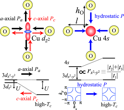
Figure 1: Bottom left: schematic variation of the $d_{z^{2}}$ orbital level with respect to that for $d_{x^{2}-y^{2}}$ under uniaxial pressure (top left inset). Bottom right: the shift of Cu$4s$ level under hydrostatic pressure and its effect on the Fermi surface.

III CALCULATION RESULTS: UNIAXIAL PRESSURE

III.1 Crystal structure under pressure

Let us begin with the case of uniaxial pressure. We first vary the lattice constants and calculate the total energy $E_{\rm tot}$. This is fit by the standard Burch-Marnaghan equationBirch to determine the most stable structure with a unit cell volume $V=V_{0}$, the $a$-axis lattice constant $a=a_{0}$, and the $c$-axis $c=c_{0}$. For simplicity, we retain the tetragonal symmetry throughout, i.e., $b=a$ (so that the $a$-compression is actually biaxial). We show in Table I the lattice parameters, $a_{0}$, $c_{0}$, $h_{\rm O}$, $h_{\rm La,Ba}$(La or Ba height measured from CuO₂ plane) and $V_{0}$, obtained for the La and Hg cuprates. The results are in good agreement with experimental values for the optimally doped compoundsLa-st ; Hg-st . We then relax the structure perpendicular to the compression direction, namely, we allow the lattice constant in that direction to relax to obtain the value that gives the lowest energy.

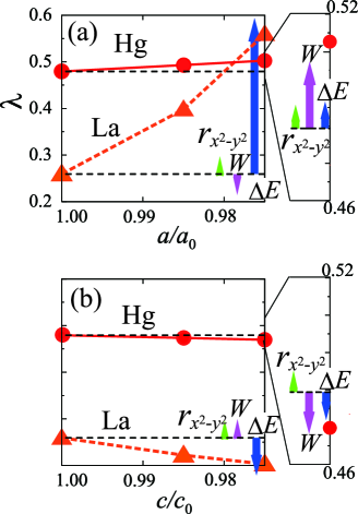
Figure 2: For uniaxial compressions the eigenvalue $\lambda$ of the Eliashberg equation is plotted against $a/a_{0}$ (a) or $c/c_{0}$ (b). Triangles (circles) indicate the result for the La (Hg) cuprates. Arrows depict the contributions (see text) to the $\lambda$ variation from $\Delta E$, $W$, and $r_{x^{2}-y^{2}}$, respectively, at $a/a_{0},c/c_{0}=0.975$. Lines are guide for the eye, with the dashed horizontal ones indicating the original values.

Figure 2 plots the eigenvalue of the Eliashberg equation $\lambda$ against the lattice compression $a/a_{0}$ and $c/c_{0}$ for each compound. The result shows that (i) in both compounds $\lambda$ increases as $a/a_{0}$ is reduced, while decreases as $c/c_{0}$ is reduced, and (ii) the absolute value of the variations of $\lambda$ is larger in La than in Hg. These features are in qualitative agreement with the experimental observations summarized in Fig.3 of ref.Hardy , which shows $\partial T_{c}/\partial P_{a}>0$ and $\partial T_{c}/\partial P_{c}<0$ for both materials, with larger $|\partial T_{c}/\partial P_{i}|$ in La than in HgHardy ; Gugenberger . To be more precise, while the compressibility in the $a$ direction is nearly the same between the two materials, that in the $c$ direction is about three times larger in Hg than in LaTakahashi ; Balagurov $(dc/dP_{c}|_{\rm Hg}\simeq 3dc/dP_{c}|_{\rm La})$, but even if we take this into account, we find that $\partial\lambda/\partial P_{c}$ is still larger for La than for Hg in our calculation.

III.2 Contribution from the $d_{z^{2}}$ orbital: $\Delta E$

Now we want to pinpoint the origin of this $T_{c}$ variation against uniaxial pressures. In both materials, $\Delta E\equiv E_{dx^{2}-y^{2}}-E_{dz^{2}}$ increases as $a/a_{0}$ is reduced, while it decreases when $c/c_{0}$ is reduced. This is natural, since the $a$ $(c)$ reduction pushes the in-plane (out-of-plane) ligands toward Cu, resulting in a larger (smaller) crystal-field splitting and hence larger (smaller) $\Delta E$PRB , as schematically depicted in Fig.1. One might then expect that this alone is the origin of the $T_{c}$ variation, since $\Delta E$ and $T_{c}$ are positively correlatedPRL . To see if this is indeed the case, we have considered a case where we increase $\Delta E$ alone to its value at $a/a_{0}=0.975$ or $c/c_{0}=0.975$, and obtain $\lambda$ with FLEX. The results are indicated in Fig.2 with arrows labeled as “$\Delta E$”. In La, the resulting $\lambda$ is very close to those obtained for the actual compression, which implies that the main origin for $\lambda$ variation under uniaxial pressure comes from $\Delta E$. By contrast, for Hg, the $\Delta E$ contribution is too small to account for the actual $\lambda$ variance (see the blowups in Fig.2).

III.3 Contribution from the $4s$ orbital: $r_{x^{2}-y^{2}}$

The reason for this is that in Hg, $\Delta E$ is $\simeq 2.5$ times larger than in La (table 1), so that the effect of the $d_{z^{2}}$ orbital is tiny, while the contribution to the $T_{c}$ variation coming from other changes in the electronic structure become comparable with that from $\Delta E$. In particular, we focus on the change in the energy difference $\Delta E_{s}$ between Cu$4s$ and Cu$d_{x^{2}-y^{2}}$ orbitals. In fact, it has been shown that the Cu$4s$ orbital, which is implicitly included in the $d_{x^{2}-y^{2}}$ Wannier orbital in the present scheme, affects the second $(t_{2})$ and third $(t_{3})$ neighbor hoppingsPavarini ; Andersen ; PRL ; PRB . Note that the $4s$ orbital can be integrated out (implicitly included in the Wannier orbitals) prior to the many-body analysis, since the $4s$ orbital sits in energy well away from the Fermi level in contrast to the $d_{z^{2}}$ orbital (Fig.1)PRL ; PRB . Smaller $\Delta E_{s}$ results in larger $r_{x^{2}-y^{2}}\equiv(|t_{2}|+|t_{3}|)/|t_{1}|$ within the $d_{x^{2}-y^{2}}$ orbital sector, resulting in a more rounded Fermi surface, which degrades $d$-wave superconductivityScalapino ; PRL ; Kent ; Maier .

To show how the roundness varies with $\Delta E_{s}$, we consider a three-orbital model which explicitly includes the Cu 4s Wannier orbitals for the Hg cupratePRL ; PRB , and show in Fig.3 the Fermi surface for various values of $\Delta E_{s}=E_{{\rm Cu}4s}-E_{{\rm Cu}3d_{x^{2}-y^{2}}}$. We stress here that, while larger $\Delta E$ and larger $r_{x^{2}-y^{2}}$ (or smaller $\Delta E_{s}$) both give more rounded Fermi surface, their effects on $T_{c}$ are opposite. Under pressure, $\Delta E_{s}$ is enhanced, which in turn reduces $r_{x^{2}-y^{2}}$. In Fig.2, we show the effect of hypothetically reducing $r_{x^{2}-y^{2}}$ down to its values at $a/a_{0}=0.975$ or $c/c_{0}=0.975$. While the effect of $r_{x^{2}-y^{2}}$ is much smaller than that of $\Delta E$ in La, the two effects are found to be comparable in Hg.

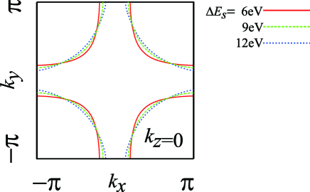
Figure 3: The Fermi surface of the three-orbital model of the Hg cuprate for values of $\Delta E_{s}$ hypothetical varied from 6eV (nearly original value) to 12eV.

III.4 Contribution from the band width: $W$

In addition to $\Delta E$ and $r_{x^{2}-y^{2}}$, the band width $W$ (the energy difference between ${\bm{k}}=(0,0)$ and $(\pi,\pi)$) of the main band is also altered by pressure. In La the change in $\lambda$ due to the modification of $W$ is small compared to that arising from $\Delta E$, but in Hg the $W$ contribution is comparable with those from $\Delta E$ and $r_{x^{2}-y^{2}}$, which in fact provides a full understanding of the net $\lambda$ variation under uniaxial pressure. Namely, the $a$ $(c)$ reduction results in an increase (decrease) of the band width as expected, which enhances (suppresses) $T_{c}$. The increase of the band width results in a suppression of $U/W$, hence the electron correlation effect. This reduces the pairing interaction, while the self-energy correction due to the spin fluctuations is reduced at the same time. The former has an effect of enhancing $T_{c}$, while the latter suppresses superconductivity. In the case of Hg compound, the latter effect supersedes the former, resulting in an enhanced $T_{c}$.

It should be noted that the contribution from $r_{x^{2}-y^{2}}$, while relatively small for uniaxial compression, enhances $T_{c}$ for both of the $a$- and $c$- axis compressions in marked contrast with the contributions from $\Delta E$ and $W$. This will become important in our analysis for hydrostatic pressures below.

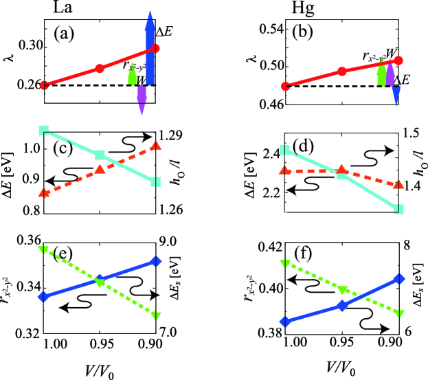
Figure 4: For hydrostatic pressure applied to La(Hg) cuprates in the left(right) column, (a),(b): The eigenvalue $\lambda$ of the Eliashberg equation plotted against the volume compression $V/V_{0}$. Arrows are as in Fig.2 for $V/V_{0}=0.90$. (c),(d): the value of $h_{\rm O}/l$(squares) and $\Delta E$(triangles). (e),(f): the value of $r_{x^{2}-y^{2}}$(triangles) and the $\Delta E_{s}\equiv E_{{\rm Cu}4s}-E_{{\rm Cu}3d_{x^{2}-y^{2}}}$(diamonds). Lines are guide for the eye.

IV CALCULATION RESULTS: HYDROSTATIC PRESSURE

IV.1 La₂CuO₄

Having identified the ingredients that determine the $T_{c}$ variation against uniaxial pressures, let us now move on to hydrostatic compression. Here we optimize the lattice structure at a fixed unit cell volume $V(<V_{0})$ by varying Poisson’s ratio, which we fit to the Burch-Marnaghan equation to obtain the most stable $E_{\rm tot}$. Notably enough, for hydrostatic pressures $\lambda$ in Fig.4 increases with the volume compression in both materials. This result qualitatively agrees with experimental resultsKlehe ; Gao . To understand its mechanism, we can, as done above for uniaxial pressures, decompose the pressure effect on $\lambda$ into the contributions from $\Delta E$, $W$, and $r_{x^{2}-y^{2}}$ (arrows in Fig. 4(a)(b)). We can then realize that the variation of $\Delta E$ against hydrostatic pressure is not as straightforward as in uniaxial pressures. Namely, we can look at $\Delta E$ along with the “aspect ratio” $h_{\rm O}/l$ against the volume reduction in Fig.4(c)(d), where $h_{\rm O}$ is the apical oxygen height and $l$ the in-plane Cu-O distance. Under hydrostatic pressure, $h_{\rm O}/l$ decreases in both materials because of the larger compressibility along the $c$ direction. One might then expect that this would reduce the crystal field splitting and hence $\Delta E$, but actually this is by no means always the case. In fact, $\Delta E$ increases with pressure for La, which is because the Cu-O distance decreases, resulting in a larger crystal-field effect. Thus the $T_{c}$ enhancement in La mainly comes from the increase of $\Delta E$.

IV.2 HgBa₂CuO₄

The above argument for La does not directly apply to Hg, since the original apical-oxygen height is larger, so that there is more room for the CuO octahedron to shrink along the $c$-axis than in La. Therefore, the $h_{\rm O}/l$ reduction is larger, resulting in a nearly constant $\Delta E$ against the decrease of $V/V_{0}$. This further makes $\Delta E$ irrelevant to the $T_{c}$ variation in Hg under hydrostatic pressures. As seen in Fig.4 with arrows, main contributions to the $T_{c}$ enhancement come from $W$ and $r_{x^{2}-y^{2}}$, with similar magnitudes. As shown in Fig.4(e)(f), the decrease of $r_{x^{2}-y^{2}}$ originally comes from an increase of the level offset $\Delta E_{s}$ introduced above. The relatively large enhancement of the Cu$4s$ level under hydrostatic pressure can be understood from Fig.1 (right), where all the ligands approaching Cu push up the energy level of the extended and isotropic Cu$4s$ orbital to a larger extent than for the localized and anisotropic Cu$3d$ orbitals. Thus a message here is the hydrostatic and uniaxial pressures exert significantly different effects. Specifically, the importance of $r_{x^{2}-y^{2}}$ becomes prominent in Hg in hydrostatic pressure because the $r_{x^{2}-y^{2}}$-contribution is positive for both of $a$- and $c$-axis compressions, while $W$-contribution has opposite effects as shown in Fig.2.

As for the band-width effect, we have found here that Hg exhibits an effect opposite to La for the present electron-electron interaction strength. To elaborate this, we have performed a FLEX calculation for various interaction strengths over $6<U/t<10$, and found that increasing the band width always results in an enhanced $\lambda$ in Hg within the considered compression range, while in La a similar effect is obtained only for $8<(U/t)$, with the effect reversing for smaller $U$. We have further noticed that this “sign change” in the band-width effect against $U$ is peculiar to the systems having smaller $\Delta E$. At any rate, the band-width effect is much smaller than the effect of $\Delta E$ in La, so that the effect of pressure-dependence of $U$ does not affect the present conclusion.

IV.3 Order of magnitude of $dT_{c}/dP$

Let us finally comment on the relation between the $\lambda$ variation for hydrostatic pressures and the $T_{c}$ enhancement in the actual pressure experiments. To see this, we have extended our calculation to lower temperatures for Hg, where $\lambda$ becomes closer to unity (i.e., $T$ approaches $T_{c}$). We find $\lambda\simeq 0.86$ at $T=0.01$ eV for $V=0.9V_{0}$, and the same value of $\lambda$ attained at $T=0.0088$ eV for $V=V_{0}$, so the temperature difference (a rough estimate of $\Delta T_{c}$) amounts to $\simeq 14$ K. Since the compressibility is $\sim 0.01$ GPa^-1Balagurov , this implies $dT_{c}/dP\sim 1$ K/GPa, which has the same order of magnitude found experimentallyHardy .

V CONCLUDING REMARKS

To summarize, we have identified the parameters that govern the $T_{c}$ variation of the single-layered cuprates under pressure. For lower-$T_{c}$ materials with small $\Delta E$ as exemplified by La₂CuO₄, $T_{c}$ is sensitive to $\Delta E$, which is identified to be the main contribution. For higher-$T_{c}$ materials with large $\Delta E$ as exemplified by HgBa₂CuO₄, $T_{c}$ is rather insensitive to $\Delta E$, and important contributions are revealed to come instead from the Fermi surface roundness governed by the Cu$4s$ orbital as well as the variation of the band width $W$. These effects coming from the electronic structure in the multi-orbital systems can be unified into a single picture in which the orbital distillation of the main band results in a higher $T_{c}$.

The present study can also shed light on a materials-science avenue for optimizing $T_{c}$. The strategy for enhancing $T_{c}$, as conceived here, is: (1) keep the level offset between the $d_{x^{2}-y^{2}}$ and $d_{z^{2}}$ orbitals large (ideally, larger than $U$ as shown in Fig.1 left), (2) expand the level offset between the Cu$4s$ and the Cu$3d_{x^{2}-y^{2}}$ as much as possible — this makes the Fermi surface more nested (fig.1 right), and (3) tune the band width $W$ to a moderate value. In this sense, it is important to keep the distance $h_{\rm O}$ between apical oxygen and Cu atom, and it is also important to decrease the in-plane Cu-O bond length $l$. In other words, the desired situation for optimizing $T_{c}$ should have an $a-b$ biaxial chemical pressure which reduces the length $l$ from those in existing compounds, with the value of $h_{\rm O}$ kept high. This may be coupled to the possibility of the level offset $\Delta E_{s}$ controlled independently of $\Delta E$ by tuning length $l$PRL .

VI ACKNOWLEDGMENTS

The numerical calculations were performed at the Supercomputer Center, ISSP, University of Tokyo. This study has been supported by Grants-in-Aid for Scientific Research from JSPS (Grants No. 23340095, RA; No. 23009446, HS; No. 21008306, HU; and No. 22340093, KK and HA). RA acknowledges financial support from JST-PRESTO. DJS acknowledges support from the Center for Nanophase Material Science at Oak Ridge National Laboratory.

References

- (1) J.D. Jorgensen, D.G. Hinks, O.Chmaissem, D.N. Argyiou, J.F. Mitchell, and B. Dabrowski, in Lecture Notes in Physics, 475, p.1 (1996).
- (2) A. Bianconi, G. Bianconi, S. Caprara, D. Di Castro, H. Oyanagi and N. L. Saini, J. Phys.: Condens. Matter 12, 10655 (2000); A. Bianconi, S. Agrestini, G. Bianconi, D. Di Castro, and N. L. Saini, J. Alloys Compd. 317-318, 537 (2001); N. Poccia, A. Ricci and A. Bianconi, Adv. Condens. Matter Phys. 2010, 261849 (2010).
- (3) S. Maekawa, J. Inoue and T. Tohyama, in The Physics and Chemistry of Oxide Superconductors, edited by Y. Iye and H. Yasuoka (Springer, Berlin, 1992), Vol. 60, pp. 105-115.
- (4) O.K. Andersen, A.I Liechtenstein, O. Jepsen, and F. Paulsen, J. Phys. Chem. Solids 56, 1573 (1995).
- (5) L.F. Feiner, J.H. Jefferson and R. Raimondi, Phys. Rev. Lett. 76, 4939 (1996).
- (6) E. Pavarini, I. Dasgupta, T. Saha-Dasgupta, O. Jepsen, and O. K. Andersen, Phys. Rev. Lett. 87, 047003 (2001).
- (7) C. Weber, K. Haule, and G. Kotliar , Phys. Rev. B 82, 125107(2010).
- (8) C. Weber, C. -H. Yee, K. Haule and G. Kotliar, arXiv:1108.3028.
- (9) T. Takimoto, T. Hotta and K. Ueda, Phys. Rev. B 69, 104504 (2004).
- (10) H. Sakakibara, H. Usui, K. Kuroki, R. Arita, and H. Aoki, Phys. Rev. Lett. 105, 057003 (2010).
- (11) H. Sakakibara, H. Usui, K. Kuroki, R. Arita and H. Aoki, Phys. Rev. B 85, 064501 (2012).
- (12) A.-K. Klehe, A. K. Gangopadhyay, J. Diederichs and J. S. Schilling Physica 213C, 266 (1993); 223C 121(1994).
- (13) L. Gao, Y. Y. Xue, F. Chen, Q. Xiong, R. L. Meng, D. Ramirez, C. W. Chu, J.H Eggert, and H.K. Mao, Phys. Rev. B 50, 4260 (1994).
- (14) F. Hardy, N. J. Hillier, C. Meingast, D. Colson, Y. Li, N. Barisic, G. Yu, X. Zhao, M. Greven, and J. S. Schilling, Phys. Rev. Lett. 105, 167002 (2010).
- (15) F. Gugenberger, C. Meingast, G.Roth, K. Grube, V. Breit, T. Weber, H. Wuhl, S. Uchida, and Y. Nakamura, Phys. Rev. B 49, 13137 (1994).
- (16) C. Meingast, A. Junod and E. Walker, Physica C 272, 106 (1996).
- (17) K. Shiraishi, A. Oshiyama, N. Shima, T. Nakayama and H. Kamimura, Solid State Commun. 66, 629-632 (1988).
- (18) H. Kamimura and M. Eto, J. Phys. Soc. Jpn. 59, 3053 (1990); M. Eto and H. Kamimura, J. Phys. Soc. Jpn. 60, 2311 (1991).
- (19) A.J. Freeman and J. Yu, Physica B 150, 50 (1988).
- (20) X. Wang, H.T. Dang, and A. J.Millis, Phys. Rev. B 84, 014530(2011).
- (21) L. Hozoi, L. Siurakshina, P. Fulde and J. van den Brink, Sci. Rep. 1, 65 (2011).
- (22) S. Uebelacker and C. Honerkamp, Phys. Rev. B 85, 155122 (2012).
- (23) M. Mori, G. Khaliullin, T. Tohyama, and S. Maekawa, Phys. Rev. Lett. 101, 247003 (2008)
- (24) P. Blaha, K. Schwarz, G.K.H. Madsen, D. Kvasnicka, and J. Luitz, Wien2k: An Augmented Plane Wave + Local Orbitals Program for Calculating Crystal Properties (Vienna University of Technology, Wien, 2001).
- (25) N. Marzari and D. Vanderbilt, Phys. Rev. B 56, 12847 (1997); I. Souza, N. Marzari and D. Vanderbilt, Phys. Rev. B 65, 035109 (2001). The Wannier functions are generated by the code developed by A. A. Mostofi, J. R. Yates, N. Marzari, I. Souza, and D. Vanderbilt, (http://www.wannier.org/).
- (26) J. Kunes, R. Arita, P. Wissgott, A. Toschi, H. Ikeda, and K. Held, Comp. Phys. Commun. 181, 1888 (2010).
- (27) N.E. Bickers, D.J. Scalapino, and S.R. White, Phys. Rev. Lett. 62, 961 (1989).
- (28) T. Dahm and L. Tewordt, Phys. Rev. Lett. 74, 793 (1995).
- (29) K. Yada and H. Kontani, J. Phys. Soc. Jpn. 74, 2161 (2005).
- (30) H. Eisaki, N. Kaneko, D. L. Feng‡, A. Damascelli, P. K. Mang, K. M. Shen, Z.-X. Shen, and M. Greven, Phys. Rev. B 69, 064512(2004).
- (31) F. Birch, Phys. Rev. B 71, 809(1947).
- (32) J. D. Jorgensen, H. -B. Schuttler, D. G. Hinks, D. W. Capone, K. Zhang, and M. B. Brodsky and D. J. Scalapino, Phys. Rev. Lett. 58, 1024 (1987).
- (33) J.L. Wagner, P.G. Radaelli, D.G. Hinks, J.D. Jorgensen, J.F. Mitchell, B. Dabrowski, G.S. Knapp, M.A. Beno, Physica C 210, 447 (1993).
- (34) H. Takahashi, H. Shaked, B. A. Hunter, P. G. Radaelli, R. L. Hitterman, D. G. Hinks, and J. D. Jorgensen , Phys. Rev. B 50, 3221 (1994).
- (35) A. M. Balagurov, D. V. Sheptyakov, V. L. Aksenov, E. V. Antipov, S. N. Putilin, P. G. Radaelli and M. Marezio, Phys. Rev. B 59, 7209 (1999).
- (36) For a review, see D.J. Scalapino in Handbook of High Temperature Superconductivity, Chapter 13, Eds. J.R. Schrieffer and J.S. Brooks (Springer, New York, 2007).
- (37) Th. Maier, M. Jarrell, Th. Pruschke, and J. Keller, Phys. Rev. Lett. 85, 1524 (2000).
- (38) P. R. C. Kent, T. Saha-Dasgupta, O. Jepsen, O. K. Andersen, A. Macridin, T. A. Maier, M. Jarrell, and T. C. Schulthess, Phys. Rev. B 78, 035132 (2008).