Neutrino cooling rates due to ^54,55,56Fe for presupernova evolution of massive stars

Abstract

Accurate estimate of neutrino energy loss rates are needed for the study of the late stages of the stellar evolution, in particular for cooling of neutron stars and white dwarfs. The energy spectra of neutrinos and antineutrinos arriving at the Earth can also provide useful information on the primary neutrino fluxes as well as neutrino mixing scenario (it is to be noted that these supernova neutrinos are emitted from a much later stage in stellar evolution than that considered in this manuscript). Proton-neutron quasi-particle random phase approximation (pn-QRPA) theory has recently being used for a microscopic calculation of stellar weak interaction rates of iron isotopes with success. Here I present the detailed calculation of neutrino and antineutrino cooling rates due to key iron isotopes in stellar matter using the pn-QRPA theory. The rates are calculated on a fine grid of temperature-density scale suitable for core-collapse simulators. The calculated rates are compared against earlier calculations. The neutrino cooling rates due to isotopes of iron are in overall good agreement with the rates calculated using the large-scale shell model. During the presupernova evolution of massive stars, from oxygen shell burning till around end of convective core silicon burning phases, the calculated neutrino cooling rates due to ⁵⁴Fe are three to four times larger than the corresponding shell model rates. The Brink’s hypothesis used in previous calculations can at times lead to erroneous results. The Brink’s hypothesis assumes that the Gamow-Teller strength distributions for all excited states are the same. It is, however, shown by the present calculation that both the centroid and total strength for excited states differ appreciably from the ground state distribution. These changes in the strength distributions of thermally populated excited states can alter the total weak interaction rates rather significantly. The calculated antineutrino cooling rates, due to positron capture and $\beta$-decay of iron isotopes, are orders of magnitude smaller than the corresponding neutrino cooling rates and can safely be neglected specially at low temperatures and high stellar densities.

1 Introduction

Despite immense technological advancements since the time when Colgate $\&$ White Col66 and Arnett Arn67 presented their classical work on energy transport by neutrinos and antineutrinos in non-rotating massive stars, the explosion mechanism of core-collapse supernovae continues to pose challenges for the collapse simulators throughout the globe. It is clear that the prompt shock that follows the bounce of the core stagnates and is not possible to cause a supernova explosion on its own. It loses energy in disintegrating iron nuclei and through neutrino emissions (mainly non-thermal) which are till then transparent to the stellar matter. A few milliseconds after the bounce, the proto-neutron star accretes mass at a few tenths of solar mass per second. This accretion, if continued even for one second, can change the ultimate fate of the collapsing core resulting into a black hole. Neutrinos are the main characters in this play and radiate around 10$\%$ of the rest mass converting the star to a neutron star. Initially the nascent neutron star is a hot thermal bath of dense nuclear matter, $e^{-}e^{+}$ pairs, photons and neutrinos. Neutrinos, having the weak interaction, are most effective in cooling and diffuse outward within a few seconds, and eventually escape with about 99$\%$ of the released gravitational energy. Despite the small neutrino-nucleus cross sections, the neutrinos flux generated by the cooling of a neutron star can produce a number of nuclear transmutations as it passes the onion-like structured envelope surrounding the neutron star. In the late-time neutrino heating mechanism the stalled shock can be revived (about 1 s after the bounce) and may be driven as a delayed explosion Bet85 . The 2D simulations (addition of convection) performed with a Boltzmann solver for the neutrino transport fails to convert the collapse into an explosion Bur03 . 2D calculations carried out in the mid -1990’s resulted in successful supernovae and revealed some role of turbulence in the collapsing gas (e.g. Fry99 ). Recently a few simulation groups (e.g. Buras06 ; Bur06 ; Woo07 have reported successful explosions in 2D mode. However a complete understanding of the explosion mechanism is still in progress. Additional energy sources were also sought that might transport energy to the mantle and lead to an explosion. Few popular sources of additional energy that were widely discussed in literature were preheating mechanism proposed by Haxton Hax88 , magnetic fields (e.g. see Ref. Kot04 ) and rotations (e.g. see Ref. Wal05 ).

The structure of the progenitor star has a vital role to play in the mechanism of the explosion. A lot many physical inputs are required at the beginning of each stage of the entire simulation process including but not limited to collapse of the core, formation, stalling and revival of the shock wave and shock propagation. It is highly desirable to calculate the presupernova stellar structure with the most reliable physical data and inputs.

Neutrinos from core-collapse supernovae are unique messengers of the microphysics of supernovae and are crucial to the life and afterlife of supernovae. They provide information regarding the neutronization due to electron capture, the infall phase, the formation and propagation of the shock wave and the cooling phase. Cooling rate is one of the crucial parameters that strongly affect the stellar evolution. During the late stages of stellar evolution a star mainly looses energy through neutrinos. White dwarfs and supernovae (which are the endpoints for stars of varying masses) have both cooling rates largely dominated by neutrino production. A cooling proto-neutron star emits about $3\times 10^{53}$ erg in neutrinos, with the energy roughly equipartitioned among all species. Further the neutrinos and antineutrinos produced as a result of nuclear reactions are transparent to the stellar matter at presupernova densities and therefore assist in cooling the core to a lower entropy state. This scenario does not necessarily hold at extremely high densities and temperatures (this would be the case for stellar collapse where dynamical time scales become shorter than the neutrino transport time scales) where neutrinos can become trapped in the so-called neutrinospheres mainly due to elastic scattering with nuclei. Prior to stellar collapse one requires an accurate determination of neutrino energy loss rates in order to perform a careful study of the final branches of star evolutionary tracks. Throughout this text (anti)neutrino energy loss rates and (anti)neutrino cooling rates are meant as the same physical phenomena and the two terms are used interchangeably. A change in the cooling rates particularly at the very last stages of massive star evolution could affect the evolutionary time scale and the iron core configuration at the onset of the explosion Esp03 . The electron capture rates and the accompanying neutrino energy loss rates are also required in determining the equation of state. The neutrino energy loss rates are important input parameters in multi-dimensional simulations of the contracting proto-neutron star. Reliable and microscopic calculations of neutrino cooling rates and capture rates can contribute effectively in the final outcome of these simulations on world’s fastest supercomputers.

The first-ever extensive calculation of stellar weak rates including the capture rates, neutrino energy loss rates and decay rates for a wide density and temperature domain was performed by Fuller, Fowler, and Newman (FFN) Ful80 . Later, Aufderheide et al. Auf94 extended the FFN work for heavier nuclei with A $>$ 60 and took into consideration the quenching of the GT strength neglected by FFN. The measured data from various (p,n) and (n,p) experiments later revealed the misplacement of the GT centroid adopted in the parameterizations of FFN. Since then theoretical efforts were concentrated on the microscopic calculations of weak-interaction mediated rates of iron-regime nuclide. Large-scale shell model (LSSM)(e.g. Lan00 ) and the proton-neutron quasiparticle random phase approximation (pn-QRPA) theory (e.g. Nab04 ) were used extensively and with relative success for the microscopic calculation of stellar weak rates. Monte Carlo shell-model is an alternative to the diagonalization method and allows calculation of nuclear properties as thermal averages (e.g. Joh92 ). However it does not allow for detailed nuclear spectroscopy and has some restrictions in its applications for odd-odd and odd-A nuclei.

The pn-QRPA theory is an efficient way to generate GT strength distributions. These strength distributions constitute a primary and nontrivial contribution to the weak-interaction mediated rates among iron-regime nuclide. Because of the high temperatures prevailing during the presupernova and supernova phase of a massive star, there is a reasonable probability of occupation of parent excited states and the total weak interaction rates have a finite contribution form these excited states. The pn-QRPA theory allows a microscopic state-by-state calculation of all these partial rates and this feature of the model greatly enhances the reliability of the calculated rates in stellar matter. Previous calculations of stellar weak-interaction rates (e.g. FFN and LSSM) assumed the so-called Brink’s hypothesis to approximate the contribution of partial rates from high-lying excited states. This hypothesis assumes that the GT strength distribution is the same as the ground-state GT strength distribution and hence the rate contribution for each transition is essentially the same. However it was shown in a recent pn-QRPA calculation Nab09 that the Brinks hypothesis is a poor approximation for key iron isotopes considered in this project. Table 2 of Ref. Nab09 showed that in the $\beta^{-}$ direction the total strength for the first excited state of ⁵⁴Fe changed from 7.56 to 6.97, that of ⁵⁵Fe increased from 6.87 to 8.87 and finally for ⁵⁶Fe decreased from 10.74 to 8.04, respectively. There were also corresponding changes in centroids and strength in $\beta^{+}$ direction. These changes do have an overall effect on the total rate under stellar conditions. Further details of these calculations and the pn-QRPA model can be found in Ref. Nab10 . The improved calculation of weak-interaction mediated rates on iron isotopes was recently introduced Nab09 using the pn-QRPA theory. The improvement was attributed to a judicious choice of model parameters and incorporation of measured deformation for the even-even isotopes of iron. There the author was able to reproduce fairly well the experimental centroids and the total strength distributions in both directions (in the GT₊ direction a proton is converted to a neutron, as in electron capture or positron decay and in the GT_- direction a neutron is converted to a proton, as in positron capture or $\beta$-decay) for the even-even iron isotopes, ^54,56Fe. This paper is devoted to a detailed analysis of the neutrino and antineutrino energy loss rates due to ^54,55,56Fe in stellar matter. The neutrino cooling rates depend heavily on the calculation of the associated GT strength distribution functions. The pn-QRPA calculated GT strength functions for iron isotopes were also introduced in Ref. Nab09 (see also Nab10 for a discussion of the subject). Simulation results of presupernova evolution of massive stars do point ^54,55,56Fe as key iron isotopes whose weak-interaction mediated rates can strongly influence the outcome of such results (e.g. see Refs. Auf94 ; Heg01 ) At lower temperatures and densities characteristic of the hydrostatic phases of stellar evolution, accurate and reliable stellar weak rates are required to determine the nucleosynthesis of nuclear species, the overall neutrino energy loss rates which may affect the temperature of the core (at relevant temperatures and densities the nonthermal neutrinos are transparent to the stellar matter), and the detailed $Y_{e}$ which becomes very important going into the core collapse. For the later phases of silicon burning to the collapse phase, overall neutronisation rates and neutrino production rates become the most interesting quantities Ful80 (during this phase the total GT_± strengths become more important rather than their distributions).

The paper is written in the following format. Section 2 describes the essential formalism for the calculation of neutrino and antineutrino energy loss rates using the pn-QRPA theory. I present my calculation in Section 3 where I also compare them with earlier calculations of neutrino energy loss rates. I summarize the main points and conclude finally in Section 4.

2 Formalism

The QRPA theory considers the residual correlations among the nucleons via one particle one hole (1p-1h) excitations in a large model space and is an efficient way to generate GT strength distributions. Kar et al. Kar94 pointed out much earlier that the quasiparticle random phase approximation (QRPA) method is quite successful in predicting the weak interaction rates of ground states all over the periodic table and also stressed the need to extend these methods to non-zero temperature domains relevant to presupernova and supernova conditions. Nabi and Klapdor-Kleingrothaus Nab99 later used the pn-QRPA theory in stellar matter to calculate contributions to weak interaction rates from parent excited states. The basic formalism of the pn-QRPA model can be found in Ref. Nab10

The neutrino (antineutrino) energy loss rates can occur through four different weak-interaction mediated channels: electron and positron emissions, and, continuum electron and positron captures. The neutrino energy loss rates were calculated using the formula

$$\lambda^{{}^{\nu(\bar{\nu})}}_{ij}=\left[\frac{\ln 2}{D}\right]\left[f_{ij}^{\nu}(T,\rho,E_{f})\right]\left[B(F)_{ij}+\left({\raise 3.01385pt\hbox{$g_{A}$}\!\mathord{\left/{\vphantom{g_{A}g_{V}}}\right.\kern-1.2pt}\!\lower 3.01385pt\hbox{$g_{V}$}}\right)^{2}_{eff}B(GT)_{ij}\right].$$ (1)

Reduced transition probabilities as well as values of constants used in Eqt. 1 can be seen from Ref. Nab10 . A quenching factor of 0.6 was introduced in the calculation Nab09 ; Nab10 . The $f_{ij}^{\nu}$ are the phase space integrals and are functions of stellar temperature ($T$), density ($\rho$) and Fermi energy ($E_{f}$) of the electrons. They are explicitly given by

$$f_{ij}^{\nu}\,=\,\int_{1}^{w_{m}}w\sqrt{w^{2}-1}(w_{m}\,-\,w)^{3}F(\pm Z,w)(1-G_{\mp})dw,$$ (2)

and by

$$f_{ij}^{\nu}\,=\,\int_{w_{l}}^{\infty}w\sqrt{w^{2}-1}(w_{m}\,+\,w)^{3}F(\pm Z,w)G_{\mp}dw.$$ (3)

In above equation $w$ is the total energy of the electron including its rest mass, $w_{l}$ is the total capture threshold energy (rest+kinetic) for positron (or electron) capture. F($\pm$ Z,w) are the Fermi functions and were calculated according to the procedure adopted by Gove and Martin Gov71 . G_± is the Fermi-Dirac distribution function for positrons (electrons).

$$G_{+}=\left[\exp\left(\frac{E+2+E_{f}}{kT}\right)+1\right]^{-1},$$ (4)

$$G_{-}=\left[\exp\left(\frac{E-E_{f}}{kT}\right)+1\right]^{-1},$$ (5)

here $E$ is the kinetic energy of the electrons and $k$ is the Boltzmann constant.

For the decay channel Eqt. 2 was used for the calculation of phase space integrals. Upper signs were used for the case of electron emissions and lower signs for the case of positron emissions. Regarding the capture channels, I used Eqt. 3 for the calculation of phase space integrals keeping upper signs for continuum electron captures and lower signs for continuum positron captures. Details of the calculation of reduced transition probabilities can also be found in Ref. Nab99a .

The total neutrino energy loss rate per unit time per nucleus is given by

$$\lambda^{\nu}=\sum_{ij}P_{i}\lambda_{ij}^{\nu},$$ (6)

where $\lambda_{ij}^{\nu}$ is the sum of the electron capture and positron decay rates for the transition $i\rightarrow j$ and $P_{i}$ is the probability of occupation of parent excited states which follows the normal Boltzmann distribution.

On the other hand the total antineutrino energy loss rate per unit time per nucleus is given by

$$\lambda^{\bar{\nu}}=\sum_{ij}P_{i}\lambda_{ij}^{\bar{\nu}},$$ (7)

where $\lambda_{ij}^{\bar{\nu}}$ is the sum of the positron capture and electron decay rates for the transition $i\rightarrow j$.

The summation over all initial and final states was carried out until satisfactory convergence in the rate calculation was achieved. The pn-QRPA theory allows a microscopic state-by-state calculation of both sums present in Eqts. 6 and 7. This feature of the model greatly increases the reliability of the calculated rates in stellar matter where there exists a finite probability of occupation of excited states.

3 Results and comparison

The improved calculation of GT_± strength distributions for ^54,55,56Fe was introduced in Ref. Nab09 and discussed in detail in Ref. Nab10 . There I also compared the calculated strength functions against the measured distributions for the case of even-even isotopes of iron. It was shown in Table 1 of Ref. Nab09 that the comparison of the total GT strengths and centroids of ^54,56Fe with the measured data improved considerably relative to the earlier pn-QRPA calculation Nab04 .

The summed B(GT₊) distributions for isotopes of iron were discussed in Ref. Nab09 . Here I show the cumulative strength distributions, B(GT_-), of ^54,55,56Fe using the pn-QRPA theory. The cumulative B(GT_-) strength distributions for the iron isotopes are displayed in Figs. 1–3. The abscissas refer to energy in daughter cobalt isotopes. It is to be noted that the distributions are well fragmented and extend to high excitation energies in daughter. The corresponding GT₊ strengths are understandably lower in magnitude as compared to the GT_- strength. The values of the total strength functions and centroids for the ground-state and excited state GT strength functions, B(GT_±), were given earlier in Ref. Nab09 .

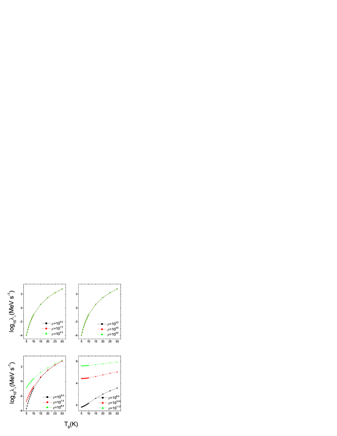
Figure 4: (Color online) Neutrino energy loss rates due to ⁵⁴Fe, as a function of stellar temperatures, for different selected densities . Densities are in units of $gcm^{-3}$. Temperatures are given in $10^{9}$ K and log${}_{10}\lambda_{\nu}$ represents the log (to base 10) of neutrino energy loss rates in units of $MeV.sec^{-1}$.

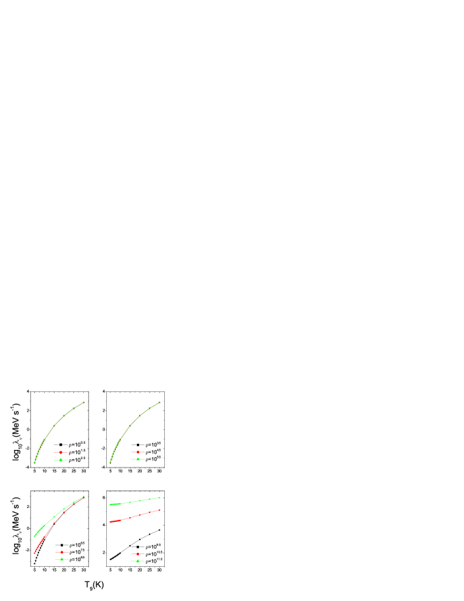
Figure 5: (Color online) Neutrino energy loss rates due to ⁵⁵Fe, as a function of stellar temperatures, for different selected densities . Densities are in units of $gcm^{-3}$. Temperatures are given in $10^{9}$ K and log${}_{10}\lambda_{\nu}$ represents the log (to base 10) of neutrino energy loss rates in units of $MeV.sec^{-1}$.

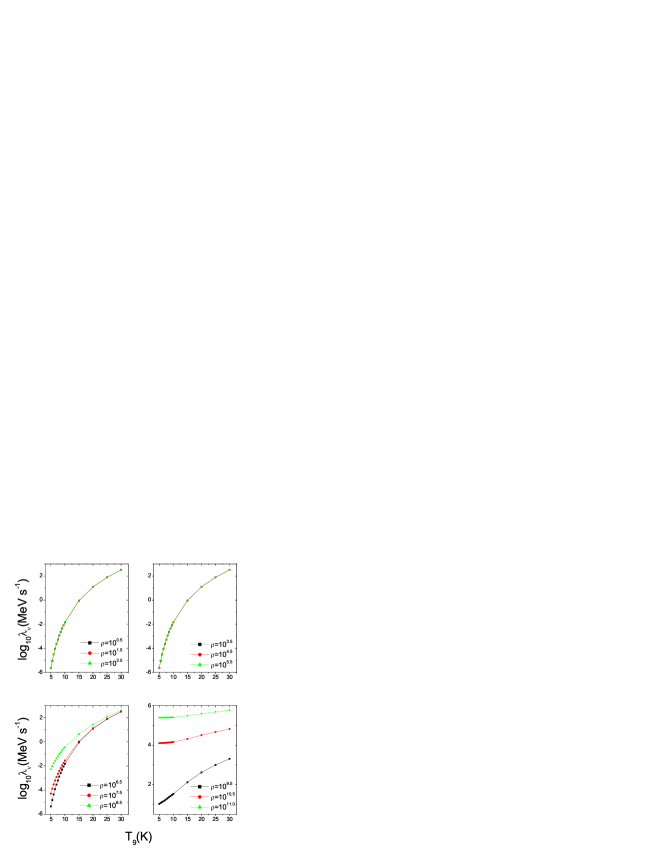
Figure 6: (Color online) Neutrino energy loss rates due to ⁵⁶Fe, as a function of stellar temperatures, for different selected densities . Densities are in units of $gcm^{-3}$. Temperatures are given in $10^{9}$ K and log${}_{10}\lambda_{\nu}$ represents the log (to base 10) of neutrino energy loss rates in units of $MeV.sec^{-1}$.

Moving on to the calculation of neutrino energy loss rates, Figs. 4–6 depict the energy loss rates for ⁵⁴Fe, ⁵⁵Fe and ⁵⁶Fe, respectively. Each figure consists of four panels depicting the calculated neutrino energy loss rates at selected temperature and density domain. It is pertinent to mention again that the neutrino energy loss rates contain contributions due to electron capture and positron decay on iron isotopes. The upper left panel, in all figures, shows the energy loss (cooling) rates in low-density region ($\rho[gcm^{-3}]=10^{0.5},10^{1.5}$ and $10^{2.5}$), the upper right in medium-low density region ($\rho[gcm^{-3}]=10^{3.5},10^{4.5}$ and $10^{5.5}$), the lower left in medium-high density region ($\rho[gcm^{-3}]=10^{6.5},10^{7.5}$ and $10^{8.5}$) and finally the lower right panel depicts the calculated rates in high density region ($\rho[gcm^{-3}]=10^{9.5},10^{10.5}$ and $10^{11}$). The neutrino energy loss rates are given in logarithmic scales (to base 10) in units of $MeV.s^{-1}$. In the figures T₉ gives the stellar temperature in units of $10^{9}$ K. One should note the order of magnitude differences in neutrino energy loss rates as the stellar temperature increases (first three panels of Figs. 4–6). For densities $\rho[gcm^{-3}]\leq 10^{8.5}$ and low stellar temperatures (T${}_{9}\leq 5$), the pn-QRPA calculates the lowest energy loss rates due to ⁵⁶Fe and highest due to ⁵⁵Fe. It can be seen from these figures that in the low density region the energy loss rates, as a function of stellar temperatures, are more or less superimposed on one another. This means that there is no appreciable change in the neutrino energy loss rates when increasing the density by an order of magnitude. There is a sharp exponential increase in the neutrino energy loss rates for the low and medium-low density regions as the stellar temperature increases up to T₉ =5. Beyond this temperature the slope of the rates reduces drastically with increasing density. For a given temperature the neutrino energy loss rates increase monotonically with increasing densities. The figures are drawn from $5\leq T_{9}\leq 30$ in order to span a smaller scale and to see the differences between the rates clearly. Neutrino cooling rates at low stellar temperatures (T${}_{9}\leq 5$) are available.

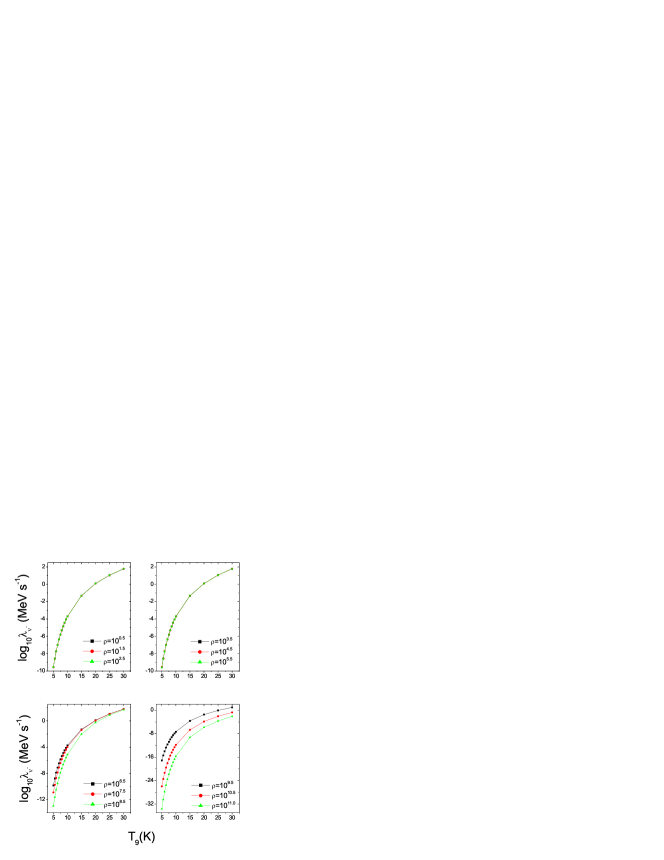
Figure 7: (Color online) Antineutrino energy loss rates due to ⁵⁴Fe, as a function of stellar temperatures, for different selected densities . Densities are in units of $gcm^{-3}$. Temperatures are given in $10^{9}$ K and log${}_{10}\lambda_{\bar{\nu}}$ represents the log (to base 10) of antineutrino energy loss rates in units of $MeV.sec^{-1}$.

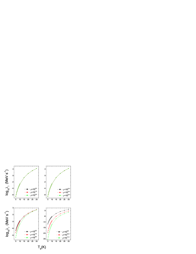
Figure 8: (Color online) Antineutrino energy loss rates due to ⁵⁵Fe, as a function of stellar temperatures, for different selected densities . Densities are in units of $gcm^{-3}$. Temperatures are given in $10^{9}$ K and log${}_{10}\lambda_{\bar{\nu}}$ represents the log (to base 10) of antineutrino energy loss rates in units of $MeV.sec^{-1}$.

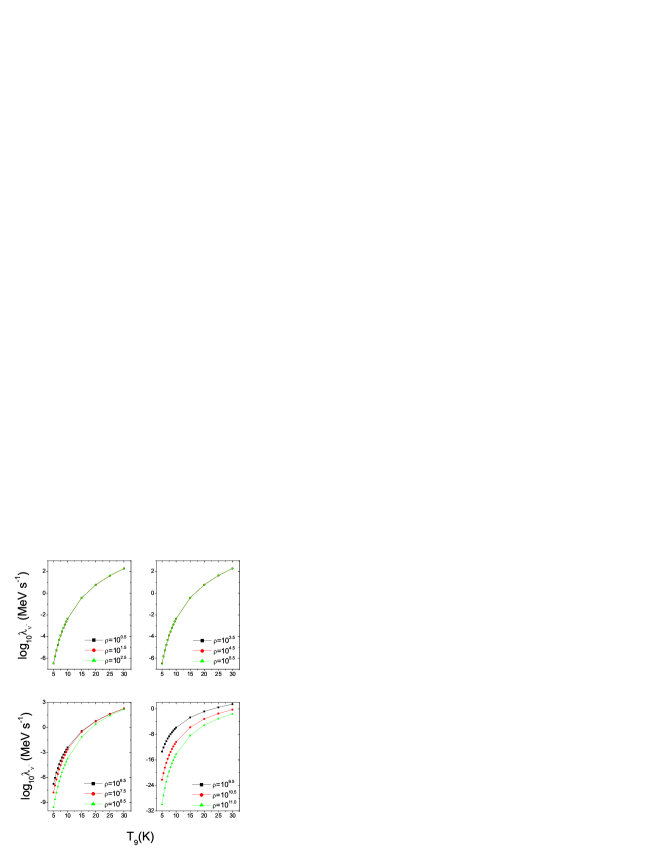
Figure 9: (Color online) Antineutrino energy loss rates due to ⁵⁶Fe, as a function of stellar temperatures, for different selected densities . Densities are in units of $gcm^{-3}$. Temperatures are given in $10^{9}$ K and log${}_{10}\lambda_{\bar{\nu}}$ represents the log (to base 10) of antineutrino energy loss rates in units of $MeV.sec^{-1}$.

The calculated antineutrino energy loss rates contain contributions due to positron capture and $\beta$-decay on iron isotopes (see Eqt. 7). Figs. 7–9 show a similar calculation for the antineutrino energy loss rates for the selected isotopes of iron. Again one notes that the figures are drawn from $5\leq T_{9}\leq 30$ due to a large variation in the magnitude of these rates as the stellar temperature increases. The anti-neutrino rates for temperatures below T${}_{9}\leq 5$ are available and can be requested from the author. Figs. 7–9 show that the corresponding anti-neutrino cooling rates are orders of magnitude smaller than the neutrino cooling rates. Specially at low temperatures and high densities these rates can safely be neglected as compared to the corresponding neutrino cooling rates. The rates are almost superimposed on one another as a function of stellar densities. However as the stellar matter moves from the medium high density region to high density region these rates start to ’peel off’ from one another. The neutrino and antineutrino energy loss rates are calculated on an extensive temperature-density grid point suitable for collapse simulations and interpolation purposes. The electronic versions of these files may be requested from the author.

An interesting query would be to know how the reported pn-QRPA calculation compares with large-scale shell model (LSSM) calculation Lan00 and the pioneer calculation performed by FFN Ful80 (specially for temperature and density domains of astrophysical interest). Of particular mention is the error in the Lanczos-based approach employed by LSSM and pointed by Pruet and Fuller Pru03 . The calculated decay rates by LSSM is a function of the number of Lanczos iterations required for convergence and this treatment of partition functions can influence their estimates of high-temperature $\beta$-decay rates. Consequently LSSM rates tend to be too low at high temperatures. The pn-QRPA calculation do not suffer from this convergence problem as it is not Lanczos-based. Secondly, as already mention, the pn-QRPA model does not assume Brink’s hypothesis and back resonances as employed in calculations by FFN and LSSM.

The comparisons are presented in a tabular form. Tables (1 – 3) show the comparison of calculated neutrino energy loss rates with those of FFN and LSSM for ⁵⁴Fe, ⁵⁵Fe and ⁵⁶Fe, respectively. Here the ratios of the calculated neutrino energy loss rates to those of LSSM, $R_{\nu}$(LSSM), and the corresponding ratios to those of FFN, $R_{\nu}$(FFN), are presented at selected temperature and density points. According to the study of presupernova evolution of massive stars by Heger and collaborators Heg01 , electron capture rates on ⁵⁴Fe are important from the oxygen shell burning phase up to the end of convective core silicon burning phase of massive stars. For temperatures (T${}_{9}\sim$3) and densities ($\rho\sim 10^{7}gcm^{-3}$) corresponding roughly to the oxygen shell burning phase of massive stars, the calculated neutrino energy loss rates due to ⁵⁴Fe are enhanced by as much as a factor of three compared to LSSM results (Table 1). The reason for this enhancement may be traced back to the three times bigger electron capture rates on ⁵⁴Fe for the corresponding density and temperature scales using the pn-QRPA theory Nab09 which dominate the production of these non-thermal neutrinos (see Eqt. 6). During the later phases of stellar evolution the pn-QRPA calculated neutrino energy loss rates are in good agreement with the LSSM rates. FFN rates are enhanced specially at low temperatures and densities by an order of magnitude. FFN neglected the quenching of the total GT strength in their rate calculation. The comparison improves at higher temperatures and densities even though the FFN rates are still enhanced (around a factor of three).

The electron capture rates on ⁵⁵Fe are most effective during the oxygen shell burning till around the ignition of the first stage of convective silicon shell burning of massive stars Heg01 . Correspondingly one should expect the most effective cooling contribution due to ⁵⁵Fe during the above mentioned phases of stellar evolution. For the corresponding temperatures (T${}_{9}\sim$3) and densities ($\rho\sim 10^{7}gcm^{-3}$), the pn-QRPA rates are in very good agreement with the LSSM rates (Table 2). In fact the overall agreement is excellent at all temperatures and densities for the case of ⁵⁵Fe. The comparison is fair with FFN rates at low temperatures and densities (though the FFN rates are slightly bigger). At high temperatures and densities FFN rates are much enhanced due to above mentioned reason.

The overall comparison of neutrino cooling rates with LSSM is again good for the case of ⁵⁶Fe (Table 3). It is to be noted that both pn-QRPA theory and LSSM calculates the ground-state GT distributions microscopically. For higher lying excited states, pn-QRPA model again calculates the GT strength distributions in a microscopic fashion whereas Brink’s hypothesis and back resonances are employed in LSSM and FFN calculations. Accordingly, whenever ground state rates command the total rate, the two calculations are found to be in excellent agreement. For cases where excited state partial rates influence the total rate, differences are seen between the two calculations. FFN rates are again enhanced by a factor of two to four as compared to pn-QRPA rates.

A similar tabular comparison of the calculation of antineutrino energy loss rates on iron isotopes using the pn-QRPA theory against FFN and LSSM rates is presented in Tables (4 – 6). Here also the ratios of the calculated antineutrino energy loss rates to those of FFN, $R_{\bar{\nu}}$(FFN), and LSSM, $R_{\bar{\nu}}$(LSSM), are presented at selected temperature and density points. For T${}_{9}=1$ and $\rho=10^{11}gcm^{-3}$ all three calculations reported cooling rates $<10^{-100}$ MeV/s and as such determination of ratios were not possible. The calculated anti-neutrino cooling rates are smaller by 1–4 orders of magnitude in comparison to previous calculations. Only at high temperatures (T${}_{9}\sim$ 30) is the pn-QRPA calculated anti-neutrino cooling rates an order of magnitude bigger than the corresponding LSSM rates.

Table 4 presents the comparison of the calculations of antineutrino energy loss rate for the case of ⁵⁴Fe. One sees that the comparison is fairly good against LSSM and FFN calculations at high temperatures (T${}_{9}\geq 10$). At low temperatures (T${}_{9}\leq 1$) and densities ($\rho\leq 10^{3}gcm^{-3}$) the calculated antineutrino cooling rates are $<$ 10^-45 MeV/s. As the density increases to $\rho=10^{11}gcm^{-3}$ the calculated rates are smaller than 10^-100 MeV/s. These small numbers are fragile functions of calculated energy levels and are around four orders of magnitude smaller than previously calculated. As the stellar temperature increases to T${}_{9}=3$, the magnitude of the calculated rates increase to around 10^-15 MeV/s for densities up to $\rho=10^{3}gcm^{-3}$, and the pn-QRPA calculated rates are around two orders of magnitude smaller (at high stellar densities, $\rho=10^{11}gcm^{-3}$, the calculated cooling rates are smaller than 10^-55 MeV/s and three orders of magnitude smaller than previous calculations). As temperature further increases so does the magnitude of calculated cooling rates and get in reasonable comparison with FFN and LSSM numbers. At high temperatures, T${}_{9}=30$, the calculated rates are around a factor six bigger than LSSM rates (it is to be recalled that LSSM calculated rates tend to be smaller at high temperatures due to Lanczos-based approach as pointed by Pruet and Fuller Pru03 ).

The calculated anti-neutrino cooling rates due to ⁵⁵Fe are 2–4 orders of magnitude smaller than previous calculations whenever they have a very small magnitude (see Table 5). According to the study by Heger et al. Heg01 , ⁵⁵Fe is included among the top three nuclei that increases $Y_{e}$ the most for 25 $M_{\odot}$ and 40 $M_{\odot}$ stars and are most effective during the silicon burning phase of these massive stars. It was later shown by Nabi in Ref. Nab10 that $\beta$-decay rates of iron isotopes were 3–5 orders of magnitude smaller than previously calculated (mainly because of approximations like Brink’s hypothesis and back resonances employed in these calculations) and hence irrelevant for the determination of the evolution of $Y_{e}$ during the presupernova phases of massive stars. During this phase (T${}_{9}\sim$3, $\rho\sim 10^{7}gcm^{-3}$) the calculated corresponding antineutrino energy loss rates are suppressed by around two orders of magnitude compared with those of LSSM and FFN (Table 5). For temperatures around $3\leq T_{9}\leq 10$, the calculated antineutrino energy loss rates are in very good comparison with LSSM rates in low-density regions. An order of magnitude enhancement is noted in calculated rates at T${}_{9}\sim$ 30 compared to LSSM numbers for reasons mentioned above. The corresponding comparison with FFN is good at high temperatures.

The comparison of antineutrino energy rates due to ⁵⁶Fe is overall fine against LSSM rates with reasonable enhancements and suppressions of calculated rates at different points of temperature and density scale (Table 6). The comparison improves at higher temperatures. The LSSM rates are enhanced up to two orders of magnitude at low temperatures. At high temperatures the calculated rates are enhanced around a factor of six. The rates are in good comparison with FFN calculation at T${}_{9}=30$. Otherwise FFN rates are enhanced by 1 –4 orders of magnitude. As mentioned earlier, the antineutrino cooling rates are smaller than the corresponding neutrino cooling rates by orders of magnitude and these small numbers can change appreciably by a mere change of 0.5 MeV in phase space calculations and are actually more reflective of the uncertainties in calculation of the energy eigenvalues (for both parent and daughter states)in the respective models.

4 Summary and conclusions

In order to understand the supernova explosion mechanism international collaborations of astronomers and physicists are being sought. Weak interaction mediated rates are key nuclear physics input to simulation codes and a reliable and microscopic calculation of these rates (both from ground-state and excited states) is desirable. The pn-QRPA theory with improved model parameters was used to calculate the (anti)neutrino energy loss rates due to iron isotopes in stellar matter. The calculation was performed in a luxurious model space of 7$\hbar\omega$. The microscopic calculation of GT_± strength distributions from ground and excited states highlighted the fact that the Brink’s hypothesis and back resonances may not be good approximations to use in calculation of stellar weak rates.

The associated energy loss rates due to weak interactions on iron isotopes in stellar matter were calculated using the pn-QRPA theory. Deformations of nuclei were taken into account and the calculation took into consideration the experimental deformations for even-even isotopes of iron (^54,56Fe). All available experimental data were incorporated in the calculation to enhance the reliability of cooling rates. The calculated neutrino energy loss rates due to ⁵⁴Fe are up to four times bigger than the LSSM rates during the oxygen and silicon shell burning phases of massive stars. The comparison with LSSM gets better for successive and supernova phases of stellar evolution. During silicon shell burning for stars ($\sim 10-25M_{\odot}$) and oxygen shell burning for much heavier stars ($\sim 40M_{\odot}$) the calculated energy loss rates due to ⁵⁵Fe are in very good comparison with the LSSM rates. The results for neutrino energy loss rates due to ⁵⁶Fe are in overall good agreement with the corresponding LSSM numbers. For the silicon burning phase of massive stars, the calculated antineutrino energy loss rates are suppressed by more than two orders of magnitude compared with the LSSM calculation and hence can be safely neglected.

According to the study of presupernova evolution of heavy stars by authors in Ref. Heg01 the most important period for determining structure and lepton fraction in the core occurs during silicon shell burning. During this decisive phase of stellar evolution the pn-QRPA calculated energy loss rates due to ⁵⁴Fe are much enhanced as compared to the results of large-scale shell model calculation and favor cooler cores with lower entropies. On the other hand, during silicon burning phases of massive stars, the antineutrino energy loss rates are suppressed by two orders of magnitude compared to previous calculations and can be neglected. These information may be of use for core-collapse simulators and may contribute in the fine tuning of the temperature, entropy and the lepton-to-baryon ratio which become very important going into stellar collapse. The rates are calculated on an extensive temperature-density grid point suitable for collapse simulations and the electronic versions of these files may be requested from the author.

Acknowledgments: The author would like to acknowledge the kind hospitality provided by the Abdus Salam ICTP, Trieste, where part of this project was completed. The author also wishes to acknowledge the support of research grant provided by the Higher Education Commission Pakistan, through the HEC Project No. 20-1283.

Table 1: Ratios of calculations of neutrino energy loss rates due to ${}^{54}Fe$ at different selected densities and temperatures. $R_{\nu}$ denotes the ratio of the calculated neutrino energy loss rates to those calculated by large scale shell model (LSSM) and those calculated by Fuller and collaborators (FFN).

$T_{9}$	$R_{\nu}$(LSSM)	$R_{\nu}$(FFN)	$R_{\nu}$(LSSM)	$R_{\nu}$(FFN)	$R_{\nu}$(LSSM)	$R_{\nu}$(FFN)	$R_{\nu}$(LSSM)	$R_{\nu}$(FFN)
	$10gcm^{-3}$	$10gcm^{-3}$	$10^{3}gcm^{-3}$	$10^{3}gcm^{-3}$	$10^{7}gcm^{-3}$	$10^{7}gcm^{-3}$	$10^{11}gcm^{-3}$	$10^{11}gcm^{-3}$
1	4.68E+00	9.66E-02	4.69E+00	9.66E-02	3.96E+00	1.13E-01	8.32E-01	2.96E-01
3	2.37E+00	1.48E-01	2.37E+00	1.48E-01	2.47E+00	1.71E-01	8.30E-01	2.95E-01
10	8.15E-01	3.90E-01	8.17E-01	3.91E-01	8.34E-01	3.94E-01	8.11E-01	2.90E-01
30	1.05E+00	3.60E-01	1.05E+00	3.61E-01	1.05E+00	3.61E-01	1.01E+00	3.52E-01

Table 2: Same as Table 1, but for neutrino energy loss rates due to ${}^{55}Fe$.

$T_{9}$	$R_{\nu}$(LSSM)	$R_{\nu}$(FFN)	$R_{\nu}$(LSSM)	$R_{\nu}$(FFN)	$R_{\nu}$(LSSM)	$R_{\nu}$(FFN)	$R_{\nu}$(LSSM)	$R_{\nu}$(FFN)
	$10gcm^{-3}$	$10gcm^{-3}$	$10^{3}gcm^{-3}$	$10^{3}gcm^{-3}$	$10^{7}gcm^{-3}$	$10^{7}gcm^{-3}$	$10^{11}gcm^{-3}$	$10^{11}gcm^{-3}$
1	1.01E+00	9.86E-01	1.01E+00	9.89E-01	1.02E+00	1.01E+00	8.09E-01	1.62E-01
3	1.52E+00	3.74E-01	1.52E+00	3.75E-01	1.49E+00	3.73E-01	7.96E-01	1.62E-01
10	1.00E+00	1.39E-01	1.00E+00	1.39-E01	1.02E+00	1.39E-01	8.41E-01	1.78E-01
30	1.67E+00	3.31E-01	1.68E+00	3.32E-01	1.68E+00	3.33E-01	1.42E+00	3.25E-01

Table 3: Same as Table 1, but for neutrino energy loss rates due to ${}^{56}Fe$.

$T_{9}$	$R_{\nu}$(LSSM)	$R_{\nu}$(FFN)	$R_{\nu}$(LSSM)	$R_{\nu}$(FFN)	$R_{\nu}$(LSSM)	$R_{\nu}$(FFN)	$R_{\nu}$(LSSM)	$R_{\nu}$(FFN)
	$10gcm^{-3}$	$10gcm^{-3}$	$10^{3}gcm^{-3}$	$10^{3}gcm^{-3}$	$10^{7}gcm^{-3}$	$10^{7}gcm^{-3}$	$10^{11}gcm^{-3}$	$10^{11}gcm^{-3}$
1	8.49E-01	2.61E-01	8.49E-01	2.61E-01	9.75E-01	3.15E-01	1.08E+00	3.57E-01
3	1.04E+00	2.36E-01	1.04E+00	2.37E-01	1.08E+00	2.44E-01	1.05E+00	3.51E-01
10	8.75E-01	4.57E-01	8.77E-01	4.58E-01	8.83E-01	4.59E-01	9.95E-01	3.30E-01
30	1.12E+00	4.56E-01	1.13E+00	4.57E-01	1.13E+00	4.58E-01	1.26E+00	4.17E-01

Table 4: Same as Table 1, but for antineutrino energy loss rates due to ${}^{54}Fe$.

$T_{9}$	$R_{\bar{\nu}}$(LSSM)	$R_{\bar{\nu}}$(FFN)	$R_{\bar{\nu}}$(LSSM)	$R_{\bar{\nu}}$(FFN)	$R_{\bar{\nu}}$(LSSM)	$R_{\bar{\nu}}$(FFN)	$R_{\bar{\nu}}$(LSSM)	$R_{\bar{\nu}}$(FFN)
	$10gcm^{-3}$	$10gcm^{-3}$	$10^{3}gcm^{-3}$	$10^{3}gcm^{-3}$	$10^{7}gcm^{-3}$	$10^{7}gcm^{-3}$	$10^{11}gcm^{-3}$	$10^{11}gcm^{-3}$
1	1.50E-04	1.51E-04	1.49E-04	1.51E-04	8.75E-04	9.29E-04	–	–
3	5.07E-02	5.42E-02	5.08E-02	5.43E-02	4.33E-02	2.64E-02	5.92E-03	5.98E-03
10	6.25E-01	5.55E-01	6.27E-01	5.56E-01	6.24E-01	5.51E-01	3.48E-01	4.74E-01
30	6.03E+00	7.19E-01	6.05E+00	7.23E-01	6.07E+00	7.23E-01	5.89E+00	7.13E-01

Table 5: Same as Table 1, but for antineutrino energy loss rates due to ${}^{55}Fe$.

$T_{9}$	$R_{\bar{\nu}}$(LSSM)	$R_{\bar{\nu}}$(FFN)	$R_{\bar{\nu}}$(LSSM)	$R_{\bar{\nu}}$(FFN)	$R_{\bar{\nu}}$(LSSM)	$R_{\bar{\nu}}$(FFN)	$R_{\bar{\nu}}$(LSSM)	$R_{\bar{\nu}}$(FFN)
	$10gcm^{-3}$	$10gcm^{-3}$	$10^{3}gcm^{-3}$	$10^{3}gcm^{-3}$	$10^{7}gcm^{-3}$	$10^{7}gcm^{-3}$	$10^{11}gcm^{-3}$	$10^{11}gcm^{-3}$
1	6.87E-03	4.98E-03	6.92E-03	4.57E-03	3.15E-03	2.09E-04	–	–
3	3.69E-01	2.98E-02	3.70E-01	2.99E-02	2.89E-02	2.35E-02	5.11E-04	2.28E-02
10	8.59E-01	9.77E-02	8.61E-01	9.79E-02	8.38E-01	9.75E-02	2.13E-01	9.62E-02
30	9.40E+00	7.18E-01	9.44E+00	7.21E-01	9.42E+00	7.21E-01	9.04E+00	7.13E-01

Table 6: Same as Table 1, but for antineutrino energy loss rates due to ${}^{56}Fe$.

$T_{9}$	$R_{\bar{\nu}}$(LSSM)	$R_{\bar{\nu}}$(FFN)	$R_{\bar{\nu}}$(LSSM)	$R_{\bar{\nu}}$(FFN)	$R_{\bar{\nu}}$(LSSM)	$R_{\bar{\nu}}$(FFN)	$R_{\bar{\nu}}$(LSSM)	$R_{\bar{\nu}}$(FFN)
	$10gcm^{-3}$	$10gcm^{-3}$	$10^{3}gcm^{-3}$	$10^{3}gcm^{-3}$	$10^{7}gcm^{-3}$	$10^{7}gcm^{-3}$	$10^{11}gcm^{-3}$	$10^{11}gcm^{-3}$
1	1.42E-01	2.09E-03	1.42E-01	2.07E-03	4.48E-02	1.63E-04	–	–
3	1.89E+00	6.38E-02	1.89E+00	6.40E-02	1.66E-01	1.87E-02	8.69E-03	1.43E-01
10	1.15E+00	7.94E-02	1.15E+00	7.96E-02	1.10E+00	7.96E-02	2.27E-01	1.04E-01
30	6.50E+00	3.93E-01	6.53E+00	3.94E-01	6.53E+00	3.94E-01	6.22E+00	3.89E-01

Figure 1: Cumulative sum of the B(GT_-) values for ⁵⁴Fe. The energy scale refers to excitation energies in daughter ⁵⁴Co.

Figure 2: Cumulative sum of the B(GT_-) values for ⁵⁵Fe. The energy scale refers to excitation energies in daughter ⁵⁵Co.

Figure 3: Cumulative sum of the B(GT_-) values for ⁵⁶Fe. The energy scale refers to excitation energies in daughter ⁵⁶Co.

References

- (1) Colgate S. A. & White R. , The hydrodynamic behavior of supernovae explosions, Astrophys. J., 143, 626-681, 1966.
- (2) Arnett W. D., Mass dependence in gravitational collapse of stellar cores, Can. J. Phys., 45, 1621 1641, 1967.
- (3) Bethe H. A. & Wilson J. R. , Revival of a stalled supernova shock by neutrino heating, Astrophys. J., 295, 14-23, 1985.
- (4) Buras R., Rampp M., Janka H.-T. & Kifonidis K., Improved models of stellar core collapse and still no explosions: What is missing?, Phys. Rev. Lett., 90, 241101, 2003.
- (5) Fryer C. L., Mass limits for black hole formation, Astrophys. J. Astrophys. J., 522, 413-418, 1999.
- (6) Buras R., Janka H.-T., Rampp M. & Kifonidis K., Two-dimensional hydrodynamic core-collapse supernova simulations with spectral neutrino transport - II. Models for different progenitor stars, Astron. Astrophys., 457, 281, 2006.
- (7) Burrows A., Livne E., Dessart L. & Ott C. D., Multidimensional radiation/hydrodynamic simulations of proto-neutron star convection, Astron. Astrophys., 645, 534-550, 2006.
- (8) Woosley S. E. & Heger A., Nucleosynthesis and remnants in massive stars of solar metallicity, Phys. Rep., 442, 269-283, 2007.
- (9) Haxton W. C., Neutrino heating in supernovae, Phys. Rev. Lett., 60, 1999-2002, 1988.
- (10) Kotake K., Sawai H., Yamada S. & Sato K., Magnetorotational effects on anisotropic neutrino emission and convection in core-collapse supernovae, Astrophys. J., 608, 391-404, 2004.
- (11) Walder R., Burrows A., Ott C. D., Livne E., Lichtenstadt I. & Jarrah M., Anisotropies in the neutrino fluxes and heating profiles in two-dimensional, time-dependent, multigroup radiation hydrodynamics simulations of rotating core-collapse supernovae, Astrophys. J., 626, 317-332, 2005.
- (12) Esposito S., Mangano G., Miele G., Picardi I. & Pisanti O., Neutrino energy loss rate in a stellar plasma, Nuc. Phys. B, 658, 217-253, 2003.
- (13) Fuller G. M., Fowler W. A. & Newman M. J., Stellar Weak-Interaction Rates for sd-Shell Nuclei. I. Nuclear Matrix Element Systematics with Application to 26Al and Selected Nuclei of Importance to the Supernova Problem, Astrophys. J. Suppl., 42, 447-473, 1980; Stellar Weak Interaction Rates for Intermediate Mass Nuclei. II. A = 21 to A = 60, Astrophys. J., 252, 715-740, 1982; Stellar Weak Interaction Rates for Intermediate Mass Nuclei. III. Rate Tables for the Free Nucleons and Nuclei with A = 21 to A = 60, Astrophys. J. Suppl., 48, 279-320, 1982; Stellar Weak Interaction Rates for Intermediate Mass Nuclei. IV. Interpolation Procedures for Rapidly Varying Lepton Capture Rates Using Effective log (ft)- Values, Astrophys. J., 293, 1-16, 1985.
- (14) Aufderheide M. B., Fushiki I., Woosley S. E., Stanford E. & Hartmann D. H., Search for Important Weak Interaction Nuclei in Presupernova Evolution, Astrophys. J. Suppl. Ser, 91, 389-417, 1994.
- (15) Langanke K. & Martínez-Pinedo G., Shell-Model Calculations of Stellar Weak Interaction Rates: II. Weak Rates for Nuclei in the Mass Range A = 45-65 in Supernovae Environments, Nucl. Phys., A673, 481-508, 2000.
- (16) Nabi J.-Un & Klapdor-Kleingrothaus H. V., Microscopic Calculations of Stellar Weak Interaction Rates and Energy Losses for fp- and fpg-Shell Nuclei, At. Data Nucl. Data Tables, 88, 237-476, 2004.
- (17) Johnson C. W., Koonin S. E., Lang G. H. & Ormand W. E., Monte-carlo methods for the nuclear shell-model, Phys. Rev. Lett., 69, 3157-3160, 1992.
- (18) Nabi J.-Un, Weak-Interaction-Mediated Rates on Iron Isotopes for Presupernova Evolution of Massive Stars, Eur. Phys. J. A, 40, 223-230, 2009.
- (19) Nabi J.-Un, Stellar decay rates of iron isotopes and its implications in astrophysics, Adv. Space Res., doi:10.1016/j.asr.2010.05.026, 2010.
- (20) Heger A., Woosley S. E., Martínez-Pinedo G. & Langanke K., Presupernova Evolution with Improved Rates for Weak Interactions, Astrophys. J., 560, 307-325, 2001.
- (21) Kar K., Ray R. & Sarkar S., Beta-decay rates of fp shell nuclei with a-greater-than-60 in massive stars at the presupernova stage, Astrophys. J., 434, 662-483, 1994.
- (22) Nabi J.-Un & Klapdor-Kleingrothaus H. V., Microscopic Calculations of Weak Interaction Rates of Nuclei in Stellar Environment for A = 18 to 100, Eur. Phys. J. A, 5, 337-339, 1999.
- (23) Gove N. B. & Martin M. J., Log-f Tables for Beta decay, At. Data Nucl. Data Tables, 10, 205-317, 1971.
- (24) Nabi J.-Un & Klapdor-Kleingrothaus H. V., Weak Interaction Rates of sd-Shell Nuclei in Stellar Environments Calculated in the Proton-Neutron Quasiparticle Random-Phase Approximation, At. Data Nucl. Data Tables, 71, 149-345, 1999.
- (25) Pruet J. & Fuller G. M., Estimates of stellar weak interaction rates for nuclei in the mass range A = 65–80, Astrophys. J. Suppl., 149, 189-203, 2003.