Synthesized grain size distribution in the interstellar medium

Abstract

We examine a synthetic way of constructing the grain size distribution in the interstellar medium (ISM). First we formulate a synthetic grain size distribution composed of three grain size distributions processed with the following mechanisms that govern the grain size distribution in the Milky Way: (i) grain growth by accretion and coagulation in dense clouds, (ii) supernova shock destruction by sputtering in diffuse ISM, and (iii) shattering driven by turbulence in diffuse ISM. Then, we examine if the observational grain size distribution in the Milky Way (called MRN) is successfully synthesized or not. We find that the three components actually synthesize the MRN grain size distribution in the sense that the deficiency of small grains by (i) and (ii) is compensated by the production of small grains by (iii). The fraction of each contribution to the total grain processing of (i), (ii), and (iii) (i.e., the relative importance of the three contributions to all grain processing mechanisms) is 30–50%, 20–40%, and 10–40%, respectively. We also show that the Milky Way extinction curve is reproduced with the synthetic grain size distributions.

1 Introduction

Dust grains are important in some physical processes in the interstellar medium (ISM). For example, they dominate the absorption and scattering of the stellar light, affecting the radiative transfer in the ISM. The extinction (absorption + scattering) by dust in the ISM as a function of wavelength is called extinction curve (Wickramasinghe, 1967; Hoyle and Wickramasinghe, 1991; Draine, 2003 for review). Extinction curves are important not only in basic radiative processes in the ISM but also in interpreting observational data: part of stellar light in a galaxy is scattered or absorbed by dust grains within the galaxy in a wavelength-dependent way according to the extinction curve. Therefore, to derive the intrinsic stellar spectral energy distribution of a galaxy, we always have to correct for dust extinction by considering the extinction curve (Calzetti, 2001).

Extinction curves generally reflect the grain composition and the grain size distribution. Mathis et al. (1977, hereafter MRN) show that a mixture of silicate and graphite dust, as originally proposed by Hoyle and Wickramasinghe (1969), with a grain size distribution (number of grains per grain radius) proportional to $a^{-3.5}$, where $a$ is the grain radius ($a\sim 0.001$–0.25 $\mu$m), reproduces the Milky Way extinction curve. Pei (1992) shows that the extinction curves in the Magellanic Clouds are also explained by the same power-law grain size distribution (i.e., $\propto a^{-3.5}$) with different abundance ratios between silicate and graphite. Kim et al. (1994) and Weingartner and Draine (2001) have applied more detailed fit to the Milky Way extinction curve in order to obtain the grain size distribution. Although their grain size distributions deviate from the MRN size distribution, the overall trend from small to large grain sizes roughly follows a power law with an index near to $-3.5$. Therefore, the MRN grain size distribution is still valid as a first approximation of the interstellar grain size distribution in the Milky Way.

What regulates or determines the grain size distribution? There are some possible processes that actively and rapidly modify the grain size distribution. Hellyer (1970) shows that the collisional fragmentation of dust grains finally leads to a power-law grain size distribution similar to the MRN size distribution (see also Bishop and Searle, 1983). In fact, Hirashita and Yan (2009) show that such a fragmentation and disruption process (or shattering) can be driven efficiently by turbulence in the diffuse ISM. However, they also show that grain velocities are strongly dependent on grain size; as a result, the grain size distribution does not converge to a simple power-law after shattering. Moreover, dust grains are also processed by other mechanisms. Various authors show that the increase of dust mass in the Milky Way ISM is mainly governed by grain growth through the accretion of gas phase metals onto the grains (we call elements composing dust grains “metals”). (Dwek, 1998; Inoue, 2003; Zhukovska et al., 2008; Draine, 2009; Inoue, 2011; Asano et al., 2012). In the dense ISM, coagulation also occurs, making the grain sizes larger (e.g., Hirashita and Yan, 2009). In the diffuse ISM phase, interstellar shocks associated with supernova (SN) remnants (simply called SN shocks in this paper) destroy dust grains, especially small ones, by sputtering (e.g., McKee, 1989). Shattering also occurs in SN shocks (Jones et al., 1996).

Modeling the evolution of the grain size distribution in the ISM is a challenging problem because a variety of processes are concerned as mentioned above. Those processes are also related to the multi-phase nature of the ISM. Liffman and Clayton (1989) calculate the evolution of grain size distributions by taking into account grain growth and shock destruction. However, their method could not treat disruptive and coagulative processes (i.e., shattering and coagulation). O’Donnell and Mathis (1997) also model the evolution of grain size distribution in a multi-phase ISM, taking into account shattering and coagulation in addition to the processes considered in Liffman and Clayton (1989). They use the extinction curve and the depletion of gas-phase metals as quantities to be compared with observations. Although their models are broadly successful, the fit to the ultraviolet extinction curve is poor, which they attribute to the errors caused by their adopted optical constants. They also show that inclusion of molecular clouds in addition to diffuse ISM phases improves the fit to the observed depletion, but they did not explicitly show the effects of molecular clouds on the extinction curve. Yamasawa et al. (2011) have recently calculated the evolution of the grain size distribution in the early stage of galaxy evolution by considering the ejection of dust from SNe and subsequent destruction in SN shocks. Since they focus on the early stage, they did not include other processes such as grain growth and disruption (shattering), which are important in solar-metallicity environments such as in the Milky Way (Hirashita and Yan, 2009).

Comparing theoretical grain size distributions with observations is not a trivial procedure. In a line of sight, we always observe a mixture of grains processed in various ISM phases. Therefore, a “synthetic” grain size distribution, which is made by summing typical grain size distributions in individual ISM phases with certain weights, is to be compared with observations. In this paper, we first formulate a synthetic way of reproducing the grain size distribution. Then, we carry out a fitting of synthetic grain size distributions to the observational grain size distribution, in order to obtain the relative importance of individual grain processing mechanisms. We do not model the multi-phase ISM in detail, but our fitting contains the information on the weights (i.e., relative importance) of different grain processing mechanisms, which depend on the ISM phase.

This paper is organized as follows. In Section 2, we explain our synthetic method to reconstruct the grain size distribution in the ISM. In Section 3, we fit our synthetic models to the observational grain size distribution in the Milky Way and examine if the fitting is successful or not. In Section 4, after we discuss our results, we calculate the extinction curves to examine if our synthesized grain size distributions are consistent with the observed extinction or not. In Section 5, we give our conclusions.

2 Synthetic grain size distribution

As explained in Introduction, we “synthesize” the observational grain size distribution (here, the MRN size distribution) by summing some representative grain size distributions in various ISM phases. These representative grain size distributions are explained in Section 2.1.

First, the ISM is divided into two parts: one is the part where the grain processing is occurring (called “grain-processing region”), and the other is the area where the grains already processed in the various grain-processing regions are well mixed (called “mixing region”). The mass fractions of the former and the latter regions are, respectively, $f_{\mathrm{proc}}$ and $1-f_{\mathrm{proc}}$. It is reasonable to assume that the grain size distribution in the mixing region should be the mean grain size distribution in the ISM (Section 2.2).

We assume that all grains are spherical with material density $s$; thus, the grain mass $m$ is expressed as $m=\frac{4}{3}\pi a^{3}s$. Although coagulation may produce porous grains (e.g., Ormel et al., 2009), we neglect the effects of porosity and assume all grains to be compact. Two grain species are treated in this paper; silicate and graphite. To avoid complexity arising from compound species, we treat these two species separately. This separate treatment is also practical in this paper as we (and other authors usually) assume that the observed extinction curve can be fitted with the two species (Section 4.4). Before being processed, the grain size distribution is assumed to be MRN: a power-law function with power index $-r$ ($r=3.5$), and upper and lower bounds for the grain radii (whose values are determined below) $a_{\mathrm{min}}$ and $a_{\mathrm{max}}$, respectively:

$$n_{\mathrm{MRN}}(a)={\displaystyle\frac{(4-r)\rho_{\mathrm{d}}}{\frac{4}{3}\pi s(a_{\mathrm{max}}^{4-r}-a_{\mathrm{min}}^{4-r})n_{\mathrm{H}}}}\,a^{-r}$$ (1)

for $a_{\mathrm{min}}\leq{a}\leq a_{\mathrm{max}}$. If $a<a_{\mathrm{min}}$ or $a>a_{\mathrm{max}}$, $n_{\mathrm{MRN}}(a)=0$. The grain size distribution is defined so that $n_{\mathrm{MRN}}(a)\,da$ is the number of grains whose sizes are between $a$ and $a+da$ per hydrogen nucleus. The dust mass density, $\rho_{\mathrm{d}}$, is related to the metallicity $Z$ (the mass fraction of elements heavier than helium in the ISM) and the hydrogen number density $n_{\mathrm{H}}$ as (Hirashita and Kuo, 2011)

$$\rho_{\mathrm{d}}=\frac{m_{\mathrm{X}}}{f_{\mathrm{X}}}(1-\xi)\left(\frac{Z}{\mathrm{Z}_{\odot}}\right)\left(\frac{\mathrm{X}}{\mathrm{H}}\right)_{\odot}n_{\mathrm{H}},$$ (2)

where $m_{\mathrm{X}}$ is the atomic mass of the key element X (X = Si for silicate and C for graphite), $f_{\mathrm{X}}$ is the mass fraction of X in the dust, $\xi$ is the fraction of element X in gas phase (i.e., the fraction $1-\xi$ is in dust phase), and (X/H)_⊙ is the solar abundance relative to hydrogen in number density. The metallicity is assumed to be solar ($Z=\mathrm{Z}_{\odot}$).

We fix the maximum grain radius as $a_{\mathrm{max}}=0.25~{}\mu$m (MRN). Although the lower bound of the grain size is poorly determined from the extinction curve (Weingartner and Draine, 2001), we assume that $a_{\mathrm{min}}=0.3$ nm, since a large number of very small grains are indeed necessary to explain the mid-infrared excess of the dust emission in the Milky Way (Draine and Li, 2001). For the other parameters, we follow Hirashita (2012). We assume that 0.75 of Si is condensed into silicate (i.e., $\xi=0.25$) while 0.85 (i.e., $\xi=0.15$) of C is included into graphite. Those values are roughly consistent with the observed depletion (e.g., Savage and Sembach, 1996), and reproduce the Milky Way extinction curve (Section 4.4). We adopt the following abundances for Si and C: $(\mathrm{Si/H})_{\odot}=3.55\times 10^{-5}$ and $(\mathrm{C/H})_{\odot}=3.63\times 10^{-4}$. We assume that Si occupies a mass fraction of 0.166 ($f_{\mathrm{X}}=0.166$) in silicate while C is the only element composing graphite ($f_{\mathrm{X}}=1$). We adopt $s=3.3$ and 2.26 g cm^-3 for silicate and graphite, respectively.

By using the MRN size distribution as the initial condition, we calculate the evolution of grain size distribution by the various processes treated in Section 2.1. In the numerical calculation, the grains going out of the radius range between $a_{\mathrm{min}}$ and $a_{\mathrm{max}}$ are removed from the calculation (the removed mass fraction is $<1$%). The processes considered are (i) “grain growth” – grain growth by accretion and coagulation in dense medium, (ii) “shock destruction” – destruction by sputtering in SN shocks, and (iii) “grain disruption” – grain disruption by shattering in interstellar turbulence. Shattering in SN shocks (Jones et al., 1996) could be included as a separate component, but in our framework, it is not possible to separately constrain the contributions from the two shattering mechanisms because both shattering mechanisms (turbulence and SN shocks) selectively destroy grains with $a\gtrsim 0.03~{}\mu$m and increase smaller grains, predicting similar grain size distributions. Thus, we simply assume that the size distribution of shattered grains, whatever the shattering mechanism may be, is represented by the one adopted in Section 2.1.3.

Although our fitting procedures are based on grain size distributions, we should keep in mind that observational constraints on the grain size distribution is mainly obtained by extinction curves. Weingartner & Draine (2001) performed a detailed fit to the Milky Way extinction curve. However, the grain size distributions derived by them broadly follow an MRN-like power law, although there are bumps and dips at some sizes. We will examine the consistency with the extinction curve later in Section 4.4.

2.1 Processes considered

2.1.1 Grain growth

Grain growth occurs in the dense ISM, especially in molecular clouds, through the accretion of metals (called accretion) and the sticking of grains (called coagulation). The change of grain size distribution by grain growth has been considered in our previous paper (Hirashita, 2012). The grain size distribution after grain growth is denoted as $n_{\mathrm{grow}}(a,\,t_{\mathrm{grow}})$, where $t_{\mathrm{grow}}$ is the duration of grain growth. We adopt $t_{\mathrm{grow}}=10$ and 30 Myr based on typical lifetime of molecular clouds (e.g., Lada et al., 2010). The metallicity in the Milky Way is high enough to allow complete depletion of grain-composing materials onto dust grains in $\sim 10$ Myr. Thus, the total masses of silicate and graphite become 1.33 ($=1/0.75$) and 1.18 ($=1/0.85$) times as large as the initial values, respectively (recall that the dust mass becomes $1/(1-\xi)$ times as much if all the dust grains accrete all the gas-phase metals). The difference in the grain size distribution between $t_{\mathrm{grow}}=10$ and 30 Myr is predominantly caused by coagulation rather than accretion.

2.1.2 Shock destruction

We calculate the change of grain size distribution by SN shock destruction in a medium swept by a SN shock, following Nozawa et al. (2006). All SN explosions are represented by an explosion of a star which has a mass of 20 M_⊙ at the zero-age main sequence, and the SN explosion energy is assumed to be $10^{51}$ erg. For the ISM, we adopt a hydrogen number density of 0.3 cm^-3 (since the destruction is predominant in the diffuse ISM; McKee, 1989), and solar metallicity. The calculation of grain destruction is performed until the shock velocity is decelerated down to 100 km s^-1 ($8\times 10^{4}$ yr after the explosion). We apply the material properties of Mg₂SiO₄ and carbonaceous dust in Nozawa et al. (2006) for silicate and graphite, respectively. We denote the grain size distribution after shock destruction by $n_{\mathrm{shock}}(a)$. The destroyed mass fractions of silicate and graphite are 0.38 and 0.27, respectively.

2.1.3 Disruption

Grain motions driven by interstellar turbulence lead to grain disruption (shattering) in the diffuse ISM (Yan et al., 2004; Hirashita and Yan, 2009). Among the various ISM phases, dust grains can acquire the largest velocity dispersion in a warm ionized medium (WIM). We recalculated the results of earlier workers based on our assumed initial conditions. We adopt the same grain velocity dispersions and hydrogen number density ($n_{\mathrm{H}}=0.1$ cm^-3) in the WIM as adopted in Hirashita and Yan (2009). The fragments are assumed to follow a power-law size distribution with a power index of $-3.3$ (Jones et al., 1996; Hirashita and Yan, 2009). We denote the grain size distribution after disruption as $n_{\mathrm{disr}}(a,\,t_{\mathrm{disr}})$, where $t_{\mathrm{disr}}$ is the duration of shattering in the WIM. The lifetime of WIM is estimated to be a few Myr from the recombination timescale and the lifetime of ionizing stars (Hirashita and Yan, 2009). Thus, we adopt $t_{\mathrm{disr}}=3$ and 10 Myr for our calculation in causing moderate and significant disruption.

2.2 Synthesizing the grain size distribution

In the beginning of this section, we introduced the mass fraction ($f_{\mathrm{proc}}$) of ISM hosting grains which are now being processed (“grain-processing region”). The mean grain size distribution over all the grain-processing region, $n_{\mathrm{synt}}(a)$, can be synthesized with the processed grain size distributions, $n_{\mathrm{grow}}(a,\,t_{\mathrm{grow}})$ (grain size distribution after grain growth with a growth duration of $t_{\mathrm{grow}}$), $n_{\mathrm{shock}}(a)$ (grain size distribution after shock destruction), and $n_{\mathrm{disr}}(a,\,t_{\mathrm{disr}})$ (grain size distribution after disruption with a shattering duration of $t_{\mathrm{disr}}$):

$$n_{\mathrm{synt}}(a) = f_{\mathrm{grow}}n_{\mathrm{grow}}(a,\,t_{\mathrm{grow}})+f_{\mathrm{disr}}n_{\mathrm{disr}}(a,\,t_{\mathrm{disr}})$$ (3)

$$+f_{\mathrm{shock}}n_{\mathrm{shock}}(a),$$

where $f_{\mathrm{grow}}$, $f_{\mathrm{disr}}$ and $f_{\mathrm{shock}}$ are the mass fractions of medium hosting, respectively, grain growth, disruption, and grain destruction in the grain-processing region. We call $n_{\mathrm{synt}}(a)$ “synthetic grain size distribution”. If both species are spatially well mixed, they would have common values for $f_{\mathrm{grow}}$, $f_{\mathrm{shock}}$, and $f_{\mathrm{disr}}$.

The mean grain size distribution in the ISM is denoted as $n_{\mathrm{mean}}(a)$ and expressed as

$$n_{\mathrm{mean}}(a)=(1-f_{\mathrm{proc}})n_{\mathrm{mean}}(a)+f_{\mathrm{proc}}n_{\mathrm{synt}}(a),$$ (4)

since it is assumed that the grain size distribution in the mixing region has already become the mean grain size distribution. By assumption, the mean size distribution is MRN: $n_{\mathrm{mean}}(a)=n_{\mathrm{MRN}}(a)$. This condition is equivalent to

$$n_{\mathrm{synt}}(a)=n_{\mathrm{MRN}}(a).$$ (5)

In the Milky Way ISM, since the grain mass is roughly in equilibrium between the growth in clouds and the destruction by SN shocks (Inoue, 2011), we apply $f_{\mathrm{grow}}R_{1}=f_{\mathrm{shock}}R_{2}$, where $R_{1}$ is the fraction of dust mass growth in clouds (0.33 and 0.18 for silicate and graphite, respectively; Section 2.1.1), and $R_{2}$ is the destroyed fraction of dust in a SN blast (0.38 and 0.27 for silicate and graphite, respectively; Section 2.1.2). Thus, we put a constraint,

$$f_{\mathrm{shock}}=(R_{1}/R_{2})f_{\mathrm{grow}}.$$ (6)

We approximately adopt $R_{1}/R_{2}=0.8$ as a mean value between silicate and graphite. As mentioned above, if the two species (silicate and graphite) are spatially well mixed, both species would have common values for $f_{\mathrm{grow}}$, $f_{\mathrm{shock}}$, and $f_{\mathrm{disr}}$. Thus, we adopt a single value for $R_{1}/R_{2}$.

Using the above constraints, Eq. (3) is reduced to

$$n_{\mathrm{synt}}(a)=f_{\mathrm{grow}}n_{\mathrm{g,s}}(a)+f_{\mathrm{disr}}n_{\mathrm{disr}}(a,\,t_{\mathrm{disr}}),$$ (7)

where $n_{\mathrm{g,s}}(a)\equiv n_{\mathrm{grow}}(a,\,t_{\mathrm{grow}})+(R_{1}/R_{2})n_{\mathrm{shock}}(a)$. Thus, we treat $f_{\mathrm{grow}}$ and $f_{\mathrm{disr}}$ as free parameters. We define the sum of all the fractions as

$$f_{\mathrm{tot}} \equiv f_{\mathrm{grow}}+f_{\mathrm{shock}}+f_{\mathrm{disr}}$$ (8)

$$= \left(1+\frac{R_{1}}{R_{2}}\right)f_{\mathrm{grow}}+f_{\mathrm{disr}}.$$

If the grain size distribution is predominantly modified by the three processes considered in this paper, we expect that $f_{\mathrm{tot}}=1$. The deviation of $f_{\mathrm{tot}}$ from 1 is an indicator of goodness of our assumption that the grain size distribution is modified by the three processes.

2.3 Best fitting parameters

We search for a set of parameters, $(f_{\mathrm{grow}},f_{\mathrm{disr}})$, which minimizes the square of the difference:

$$\delta^{2}=\frac{1}{N}\sum_{i=1}^{N}\,[\log n_{\mathrm{synt}}(a_{i})-\log n_{\mathrm{MRN}}(a_{i})]^{2},$$ (9)

where $a_{i}$ is the grain size sampled by logarithmic bins (i.e., $\log a_{i+1}-\log a_{i}$ is the same for any $i$), and $N$ is the number of the sampled grain radii ($N=512$ in our model, but the results are insensitive to $N$).

The individual components of processed grain size distributions [$n_{\mathrm{grow}}(a,\,t_{\mathrm{grow}})$, $n_{\mathrm{shock}}(a)$, and $n_{\mathrm{disr}}(a,\,t_{\mathrm{disr}})$] as well as $n_{\mathrm{g,s}}(a)$ for silicate and graphite are shown in Fig. 1. The MRN size distribution, which should be fitted, is also presented. Our fitting procedure is first applied separately for silicate and graphite, although we discuss a possibility that both species have common values for $(f_{\mathrm{grow}},f_{\mathrm{disr}})$ later in Section 4.

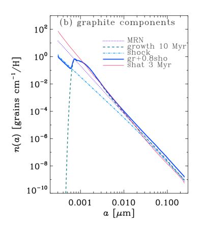
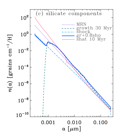
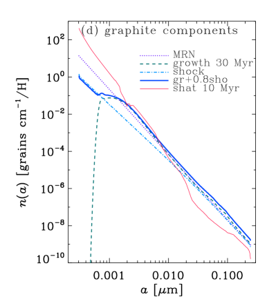
Figure 1: Individual components for synthesized grain size distributions. The thin solid, dashed, and dot-dashed lines represent individual components processed by disruption (shattering) for 3 Myr in Panels (a) and (b), and for 10 Myr in Panels (c) and (d), growth for 10 Myr in Panels (a) and (b) and for 30 Myr in Panels (c) and (d), and shock, respectively. The thick solid line shows $n_{\mathrm{g,s}}(a)=n_{\mathrm{grow}}(a,\,t_{\mathrm{grow}})+0.8n_{\mathrm{shock}}(a)$. The dotted line shows the MRN size distribution adopted in this paper. Panels (a) and (c) present silicate while Panels (b) and (d) show graphite.

3 Results

In Table 1, we show the best-fitting values of $f_{\mathrm{grow}}$ and $f_{\mathrm{disr}}$. We examine $t_{\mathrm{grow}}=30$ and 10 Myr, and $t_{\mathrm{disr}}=3$ and 10 Myr as mentioned in Section 2.1. We observe that $f_{\mathrm{grow}}=0.16$–0.55 and $f_{\mathrm{disr}}=0.06$–0.57 fit the MRN grain size distribution. The sum of all the fractions, $f_{\mathrm{tot}}$ (Eq. 8) is unity with the maximum difference of 15% (see the column of $f_{\mathrm{tot}}$ in Table 1).

Table 1: Models.

Name	species	$t_{\mathrm{grow}}$	$t_{\mathrm{disr}}$	$f_{\mathrm{grow}}$	$f_{\mathrm{disr}}$	$\delta^{2}$	$f_{\mathrm{tot}}$
		(Myr)	(Myr)			($10^{-3}$)
A	silicate	30	3	0.26	0.46	3.7	0.93
	graphite			0.43	0.24	4.2	1.01
B	silicate	10	3	0.16	0.57	16	0.86
	graphite			0.40	0.20	13	0.92
C	silicate	30	10	0.42	0.16	6.4	0.92
	graphite			0.55	0.073	7.3	1.06
D	silicate	10	10	0.40	0.15	33	0.88
	graphite			0.50	0.057	15	0.96

Note: $f_{\mathrm{shock}}=0.8f_{\mathrm{grow}}$ from Eq. (6).

In order to show how the synthetic grain size distributions reproduce the MRN size distribution, we present Fig. 2, where we only show Models A and D for the smallest and the largest residuals $\delta^{2}$. We observe that the best-fitting results are fairly consistent with the MRN size distribution. In particular, the enhanced and depleted abundances of small grains at $a\lesssim 0.001~{}\mu$m in $n_{\mathrm{disr}}$ and $n_{\mathrm{g,s}}$, respectively, cancel out very well, especially in Model A. In Model D, the synthesized size distribution slightly fails to fit the MRN around $a\sim 0.001$–$0.002~{}\mu$m because both $n_{\mathrm{g,s}}$ and $n_{\mathrm{disr}}$ (which are used for the fitting) show an excess around this grain radius range; thus, the excess around these sizes in the synthesized grain size distribution inevitably remains in Model D. However, the Milky Way extinction curve is reproduced even by Model D within a difference of $\sim 10$% (see Section 4.4).

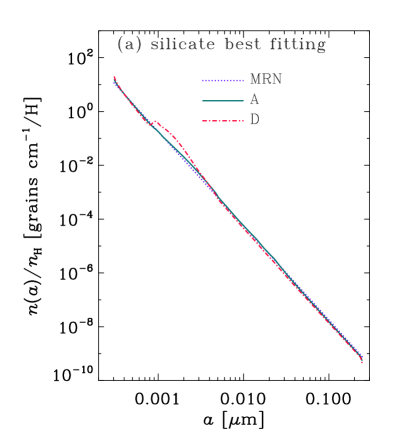
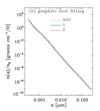
Figure 2: Best-fitting synthetic grain size distributions to the MRN size distribution. Panels (a) and (b) show silicate and graphite, respectively. We only show two models (A and D; solid and dot-dashed lines, respectively) for the smallest and largest residuals ($\delta^{2}$) among the four models. The dotted line shows the MRN size distribution.

In order to see the details of the fitting, we show the ratio between the synthesized grain size distribution and the MRN distribution in Fig. 3. There is a general trend of excess around $a\sim 0.001$–0.003 $\mu$m, which is due to grain growth (see Fig. 1). The excess is stronger in Models B and D than in Models A and C, which is why the fit is worse in Models B and D than Models A and C (Table 1). Since the bump comes from grain growth, the fit tends to suppress $f_{\mathrm{grow}}$ in the presence of a strong bump. As a result, $f_{\mathrm{tot}}$ is smaller in Models B and D than Models A and C (Table 1). We also observe in Fig. 3 that the bump appears at different grain radii between Models A/C and B/D because of the difference in the duration of grain growth. This bump may disappear if coagulation is more efficient than assumed here: more efficient coagulation may be realized if $t_{\mathrm{grow}}\gg 30$ Myr and/or coagulation also occurs in denser regions (Section 4.2).

Fig. 3 also indicates that the synthetic grain size distributions tend to be deficient at the largest grain sizes ($a\gtrsim 0.1~{}\mu$m). This is because shattering tends to process large grains into small sizes (see Fig. 1). The deficiency of large grains may be overcome if we include the supply of large grains by stellar sources of efficient coagulation as discussed in Section 4.2. Because of significant grain growth in Models A and C, the deficiency of large grains is recovered by grain growth at $a\sim 0.01$–$0.03~{}\mu$m for silicate. In Models A and C of graphite, shattering causes a dip feature around $a\sim 0.03~{}\mu$m as seen in Fig. 1, which also appears in Fig. 3. In the WIM, where shattering is assumed to occur in this paper, grains with $a\gtrsim\mbox{a few}\times 10^{-2}~{}\mu$m are accelerated up to velocities larger than the shattering threshold by turbulence. Shattering efficiently destroys small grains because of their large surface-to-volume ratios. Thus, the shattering efficiency is the largest for the smallest grains that attain a velocity above the shattering threshold. This is the reason why the grains around $a\sim 0.03~{}\mu$m are particularly destroyed by shattering. This dip feature would be smoothed out in reality since the grain velocity driven by turbulence has a dependence on grain charge, gas density, magnetic field, etc., all of which have a wide range within a galaxy.

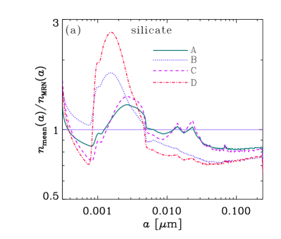
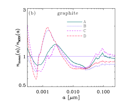
Figure 3: The ratio of the synthetic grain size distribution to the MRN size distribution. Panels (a) and (b) show silicate and graphite, respectively. The solid, dotted, dashed, and dot-dashed lines represent Models A, B, C, and D, respectively.

4 Discussion

4.1 Derived parameters

The obtained values of the parameters $f_{\mathrm{grow}}$ and $f_{\mathrm{disr}}$ reflect the fraction of individual grain processing mechanisms. In other words, these two quantities show the relative importance of grain growth and disruption. Note that the efficiency of shock destruction is automatically constrained by the balance with the mass growth by grain growth (Eq. 6). Table 1 shows that the best-fitting parameters are not very sensitive to $t_{\mathrm{grow}}$ (duration of grain growth) but that they are sensitive to $t_{\mathrm{disr}}$. For larger $t_{\mathrm{disr}}$, only a smaller $f_{\mathrm{disr}}$ is necessary because the grain size distribution is more modified. As expected, $f_{\mathrm{disr}}t_{\mathrm{disr}}$ is less sensitive to $t_{\mathrm{disr}}$; note that $f_{\mathrm{disr}}t_{\mathrm{disr}}$ is the mean duration of disruption per processed grain.

Seeing all the models, we find $f_{\mathrm{grow}}\sim 0.2$–0.6 and $f_{\mathrm{disr}}\sim 0.06$–0.6 (or $f_{\mathrm{disr}}t_{\mathrm{disr}}\sim 0.6$–1.7 Myr). As mentioned in Section 2.2, if silicate and graphite are well mixed in the ISM, they are expected to have the common values for $f_{\mathrm{grow}}$, $f_{\mathrm{shock}}$, and $f_{\mathrm{disr}}$. In this sense, Models C and D work better than Models A and B. In summary, 20–60% of processing occurs in dense clouds (i.e., grain growth), while a processed dust grain experiences disruption for $\sim 1$ Myr on average (or disruption accounts for 6–60% of processing). From the equilibrium constraint of the total dust mass (Eq. 6), the fraction of shock destruction to all the processing is $f_{\mathrm{shock}}=0.8f_{\mathrm{grow}}\sim 0.1$–0.4.

The sum of all the fractions, $f_{\mathrm{tot}}$ (Eq. 8), is unity with the maximum deviation of 15%. In other words, we cannot reject other processing mechanisms, which could contribute to the grain processing with $\lesssim 15$%.

We have shown that the grain size distributions after (i) grain growth, (ii) shock destruction, and (iii) grain disruption can synthesize the MRN size distribution. It is also likely that we can say the opposite; that is, to realize the MRN size distribution, those three processes are crucial. Without (i) the grain mass just decreases; without (ii) the grain mass just increases; without (iii) there is no mechanism that produce the large abundance of small grains.

4.2 Stellar sources?

In this paper, we did not consider dust supply from stars, because the dust mass in the Milky Way is governed by the equilibrium between grain growth in molecular clouds and grain destruction by SN shocks (e.g. Inoue, 2011). Dust grains supplied from stars may be biased to large sizes. Production of large grains from asymptotic giant branch (AGB) stars is indicated observationally (Groenewegen, 1997; Gauger et al., 1998; Höfner, 2008; Mattsson & Höfner, 2011). The dust ejected from SNe is also biased to large grain sizes because small grains are selectively destroyed by the shocked region within the SNe (Bianchi and Schneider, 2007; Nozawa et al., 2007). Coagulation associated with star formation is also a source of large grains if coagulated grains in circumstellar environments are somehow ejected into the ISM. For this possibility, Hirashita and Omukai (2009) have shown that dust grains can grow up to micron sizes by coagulation in star formation (see also Ormel et al., 2009). As mentioned in Section 3, efficient coagulation may also solve the bump problem around $a\sim 0.001$–0.003 $\mu$m. These possible sources of large grains may be worth including in dust evolution models in the future.

Table 2: Models with $f_{\mathrm{tot}}=1$.

Name	species	$t_{\mathrm{grow}}$	$t_{\mathrm{disr}}$	$f_{\mathrm{grow}}$	$f_{\mathrm{disr}}$	$\delta^{2}$	$f_{\mathrm{tot}}$
		(Myr)	(Myr)			($10^{-3}$)
A	silicate	30	3	0.19	0.45	2.1	1
	graphite			0.32	0.24	3.5	1
B	silicate	10	3	0.065	0.43	6.8	1
	graphite			0.19	0.22	6.2	1
C	silicate	30	10	0.34	0.16	4.5	1
	graphite			0.53	0.074	7.8	1
D	silicate	10	10	0.22	0.14	20	1
	graphite			0.33	0.060	10	1

Note: $f_{\mathrm{shock}}=1-f_{\mathrm{grow}}-f_{\mathrm{shock}}$.

Table 3: Models with three free parameters.

Name	species	$t_{\mathrm{grow}}$	$t_{\mathrm{disr}}$	$f_{\mathrm{grow}}$	$f_{\mathrm{shock}}$	$f_{\mathrm{disr}}$	$\delta^{2}$	$f_{\mathrm{tot}}$
		(Myr)	(Myr)				($10^{-3}$)
A	silicate	30	3	0.13	0.62	0.45	0.98	1.2
	graphite			0.20	0.76	0.25	1.8	1.2
B	silicate	10	3	0.038	0.83	0.47	2.4	1.3
	graphite			0.11	0.92	0.23	2.1	1.3
C	silicate	30	10	0.27	0.80	0.16	3.0	1.2
	graphite			0.42	0.69	0.074	6.4	1.2
D	silicate	10	10	0.16	1	0.15	10	1.3
	graphite			0.24	0.99	0.061	5.8	1.3

4.3 Fitting under other constraints

In Section 2.2, we adopted the balance between the dust mass growth by accretion and the dust mass loss by shock destruction (Eq. 6) as a constraint. Although this constraint is reasonable for the dust content in the Milky Way (e.g., Inoue, 2011), it may be useful to apply other constraints without using Eq. (6), to see how the best-fitting parameters have been controlled by Eq. (6).

First we try to fit the MRN size distribution with the three components under the condition that the sum of all the fractions is unity: $f_{\mathrm{grow}}+f_{\mathrm{shock}}+f_{\mathrm{disr}}=1$. The results with this fitting are shown in Table 2. The best-fitting values of $f_{\mathrm{disr}}$ vary from those in Table 1 within a difference of 10% except for Model B of silicate (25% less). However, the best-fitting values of $f_{\mathrm{grow}}$ is broadly 1/2–2/3 of those in Table 1. As a result, Eq. (6) is not satisfied, and the total dust mass decreases.

Next, we perform fitting to the MRN size distribution with the parameters $f_{\mathrm{grow}}$, $f_{\mathrm{shock}}$, and $f_{\mathrm{disr}}$ free. The results are shown in Table 3. Again, the values of $f_{\mathrm{disr}}$ differ by only $\lesssim 10$% except for Model B of silicate (18% less). However, $f_{\mathrm{grow}}$ is only $\sim 1/3$–2/3 of the values in Table 1, and $f_{\mathrm{shock}}$ is made large to compensate for the decreased $f_{\mathrm{grow}}$. This means that the fitting is practically dominated by the balance between the decreased small grains in shock destruction and the increased small grains in disruption (shattering). Because of the dominance of $f_{\mathrm{shock}}$, Eq. (6) is not satisfied, and the total dust mass decreases.

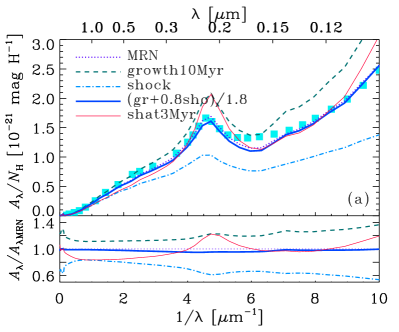
Figure 4: Upper panel: Extinction curves (extinction per hydrogen nucleus as a function of wavelength) calculated for the components used for the fitting to the grain size distribution. These components are shown in Fig. 1. The thin solid, dashed, and dot-dashed lines represent individual components processed for the following processes: disruption (shattering) for 3 Myr in Panel (a) and for 10 Myr in Panel (b), growth for 10 Myr in Panel (a) and for 30 Myr in Panel (b), and shock, respectively. The thick solid line shows the extinction curve for $n_{\mathrm{g,s}}(a)/1.8$ (divided by 1.8 because the component “g,s” contains the grain mass 1.8 times as much as the MRN). The dotted line presents the extinction curve for the MRN size distribution. The points show the observed Milky Way extinction curve taken from Pei (1992). Lower panel: Ratio of extinction curves to the extinction curve of the MRN size distribution. The line species in the lower panel correspond to those in the upper panel.

4.4 Extinction curve

The MRN grain size distribution is originally derived from the Milky Way extinction curve. Therefore, in order to check if our fitting by synthetic grain size distributions is successful or not, it is useful to calculate extinction curves.

Extinction curves are calculated by using the same optical properties of silicate and graphite as those in Hirashita and Yan (2009). The grain extinction cross section as a function of wavelength and grain size is derived from the Mie theory, and is weighted for the grain size distribution per hydrogen nucleus to obtain the extinction curve per unit hydrogen nucleus (denoted as $A_{\lambda}/N_{\mathrm{H}}$). The abundances of silicate and graphite relative to hydrogen nuclei are already inherent in the models through the abundances of Si and C and $\xi$ (Section 2).

First we show the extinction curves of the individual components, which are used to fit the MRN size distribution, in Fig. 4. Grain growth does not make the extinction curve flatter in spite of the increase of the mean grain size. The reason is already explained in Hirashita (2012): Accretion predominantly occurs at the smallest sizes. Since the extinction at short wavelengths is more sensitive to the increase of the mass of small grains than that at long wavelengths, the extinction curve becomes rather steeper. Although coagulation flattens the extinction curve, the flattening due to coagulation does not overwhelm the steepening due to the above effect of accretion.

Shock destruction makes the extinction curve flatter because small grains are more easily destroyed than large grains. Grain disruption steepens the extinction curve because of the production of a large number of small grains. The 0.22 $\mu$m bump created by small graphite grains in this model becomes also prominent by grain disruption. We also show the extinction curve for the grain size distribution $n_{\mathrm{g,s}}(a)$ (The component $n_{\mathrm{g,s}}$ has a total dust mass 1.8 times as large as the initial value. To see the difference of the extinction curve, it would be helpful to compare under the same dust mass, so $n_{\mathrm{g,s}}/1.8$ is compared with the MRN in Fig. 4.)

In Fig. 5, we show the extinction curves calculated for Models A–D. First of all, we confirm that the MRN size distribution reproduces the observed extinction curve (some small deviations can be fitted further if we adopt a more detailed functional form of the grain size distribution, which is beyond the scope of this paper; see Weingartner and Draine, 2001, for a detailed fitting). Comparing the extinction curve for the MRN size distribution and those for Models A–D, we observe that the extinction curve is reproduced within a difference of $\sim 10$%. Models A and C are successful, while Models B and D systematically underproduce the MRN extinction curve (although the difference is small). The underprediction by $\sim 10$% in Models B and D occurs because $f_{\mathrm{tot}}$ is $\sim 0.9$.

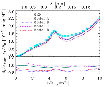
Figure 5: Extinction curves (extinction per hydrogen nucleus as a function of wavelength) calculated for Models A–D (upper panel). The ratio to the extinction curve for the MRN size distribution is also shown (lower panel). The solid, thick dotted, dashed, and dot-dashed lines represent Models A, B, C, and D, respectively. The thin dotted line shows the extinction curve for the MRN size distribution. The points show the observed Milky Way extinction curve taken from Pei (1992).

In the above, we adopted different values for $f_{\mathrm{grow}}$ and $f_{\mathrm{disr}}$ between silicate and graphite. As mentioned in Section 2.2, if both species are well mixed in the ISM, they would have common values of these parameters. In Fig. 6, we show the extinction curve by taking the average of the values for silicate and graphite (for example, $f_{\mathrm{grow}}=0.35$ and $f_{\mathrm{disr}}=0.35$ for Model A). We find that the difference between Figs. 5 and 6 is small. Therefore, the mean values work to reproduce the Milky Way extinction curves. The mean values are in the range of $f_{\mathrm{grow}}=0.3$–0.5 and $f_{\mathrm{disr}}=0.1$–0.4. We conclude that the synthetic grain size distributions with these parameter ranges reproduce the Milky Way extinction curve.

Figure 6: Same as Fig. 5 but we use the mean values between silicate and graphite for $f_{\mathrm{grow}}$ and $f_{\mathrm{disr}}$.

5 Conclusion

In our previous papers (Nozawa et al., 2006; Hirashita and Yan, 2009; Hirashita, 2012), we showed that dust grains are quickly processed by shock destruction, disruption, and grain growth. In this paper, thus, we have examined if the MRN grain size distribution, which is believed to represent the grain size distribution in the Milky Way, can be reproduced by the processed grain size distributions. We “synthesized” the grain size distribution by summing the processed grain size distributions under the condition that the decrease of dust mass by shock destruction is compensated by grain growth. We have found that the synthetic grain size distribution can reproduce the MRN grain size distribution in the sense that the deficiency of small grains by grain growth and shock destruction can be compensated by the production of small grains by disruption. The values of the fitting parameters indicate that, among the processed grains, 30–50% is growing in dense medium, 20–40% is being destroyed by shocks in diffuse medium, and 10–40% is being shattered in diffuse medium (the percentage shows the relative importance of each process). The extinction curves calculated by the synthesized grain size distributions reproduce the observed Milky Way extinction curve within a difference of $\sim 10$%. This means that our idea of synthesizing the grain size distribution based on major processing mechanisms (i.e., grain growth, shock destruction, and disruption) is promising as a general method to “reconstruct” the extinction curve.

- [1] Asano, R. S., Takeuchi, T. T., Inoue, A. K., and Hirashita, H., Dust formation history of galaxies: a critical role of metallicity for the grain growth by accreting metals in the interstellar medium, Earth Planets Space, submitted, 2012.
- [2] Bianchi, S. and Schneider, R., Dust formation and survival in supernova ejecta, Mon. Not. R. Astron. Soc., 378, 973–982, 2007.
- [3] Bishop, J. E. L. and Searle, T. M., Power-law asymptotic mass distributions for systems of accreting or fragmenting bodies, Mon. Not. R. Astron. Soc., 203, 987–1009, 1983.
- [4] Calzetti, D., The Dust Opacity of Star-forming Galaxies, Publications of the Astronomical Society of the Pacific, 113, 1449–1485, 2001
- [5] Draine, B. T., Interstellar Dust Grains, Annual Reviews of Astronomy and Astrophysics, 41, 241–289, 2003
- [6] Draine, B. T. and Li, A., Infrared Emission from Interstellar Dust. I. Stochastic Heating of Small Grains, Astrophysical Journal, 551, 807–824, 2001.
- [7] Dwek, E., The Evolution of the Elemental Abundances in the Gas and Dust Phases of the Galaxy, Astrophysical Journal, 501, 643–665, 1998.
- [8] Gauger, A., Balega, Y. Y., Irrgang, P., Osterbart, R., and Weigelt, G., High-resolution speckle masking interferometry and radiative transfer modeling of the oxygen-rich AGB star AFGL 2290, Astronomy and Astrophysics, 346, 505–519, 1998.
- [9] Groenewegen, M. A. T., IRC +10 216 revisited. I. The circumstellar dust shell, Astronomy and Astrophysics, 317, 503–520, 1997.
- [10] Hellyer, B., The fragmentation of the asteroids, Mon. Not. R. Astron. Soc., 148, 383–390, 1970.
- [11] Hirashita, H., Dust growth in the interstellar medium: How do accretion and coagulation interplay?, Mon. Not. R. Astron. Soc., in press, 2012.
- [12] Hirashita, H., and Kuo, T.-M., Effects of grain size distribution on the interstellar dust mass growth, Mon. Not. R. Astron. Soc., 416, 1795–1801, 2011.
- [13] Hirashita, H., and Omukai, K., Dust coagulation in star formation with different metallicities, Mon. Not. R. Astron. Soc., 399, 1795–1801, 2009.
- [14] Hirashita, H. and Yan, H., Shattering and coagulation of dust grains in interstellar turbulence, Mon. Not. R. Astron. Soc., 394, 1061–1074, 2009.
- [15] Höfner, S., Winds of M-type AGB stars driven by micron-sized grains, Astronomy and Astrophysics, 491, L1–L4, 2008.
- [16] Hoyle, F. and Wickramasinghe, N. C., Interstellar Grains, Nature, 223, 450–462, 1969.
- [17] Hoyle, F. and Wickramasinghe, N. C., The Theory of Cosmic Grains, Kluwer Academic Publishers, Dordrecht, 1991.
- [18] Inoue, A. K., Evolution of Dust-to-Metal Ratio in Galaxies, Publications of the Astronomical Society of Japan, 55, 901–909, 2003.
- [19] Inoue, A. K., The origin of dust in galaxies, Earth Planets Space, 63, 1027–1039, 2011.
- [20] Jones, A., Tielens, A. G. G. M., and Hollenbach, D., Astrophysical Journal, Grain Shattering in Shocks: The Interstellar Grain Size Distribution, 469, 740–764, 1996.
- [21] Kim, S.-H., Martin, P. G., and Hendry, P. D., The size distribution of interstellar dust particles as determined from extinction, Astrophysical Journal, 422, 164–175, 1994.
- [22] Lada, C. J., Lombardi, M., and Alves, J. F., On the Star Formation Rates in Molecular Clouds, Astrophysical Journal, 724, 687–693, 2010.
- [23] Liffman, K. and Clayton, D. D., Stochastic evolution of refractory interstellar dust during the chemical evolution of a two-phase interstellar medium, Astrophysical Journal, 340, 853–868, 1989.
- [24] Mathis, J. S., Rumpl, W., and Nordsieck, K. H., The size distribution of interstellar grains, Astrophysical Journal, 217, 425–433, 1977 (MRN).
- [25] Mattsson, L. and Höfner, S., Dust-driven mass loss from carbon stars as a function of stellar parameters. II. Effects of grain size on wind properties, Astronomy and Astrophysics, 533, A42, 2011.
- [26] McKee, C. F., Dust destruction in the interstellar medium, in Interstellar Dust, Proc. of IAU 135, Edited by L. J. Allamandola & A. G. G. M. Tielens, 431–443, Kluwer, Dordrecht, 1989.
- [27] Nozawa, T., Kozasa, T., and Habe, A., Dust Destruction in the High-Velocity Shocks Driven by Supernovae in the Early Universe, Astrophysical Journal, 648, 435–451, 2006.
- [28] Nozawa, T., Kozasa, T., Habe, A., Dwek, E., Umeda, H., Tominaga, N., Maeda, K., and Nomoto, K., Evolution of Dust in Primordial Supernova Remnants: Can Dust Grains Formed in the Ejecta Survive and Be Injected into the Early Interstellar Medium?, Astrophysical Journal, 666, 955–966, 2007.
- [29] O’Donnell, J. E. and Mathis, J. S., Dust Grain Size Distributions and the Abundance of Refractory Elements in the Diffuse Interstellar Medium, Astrophysical Journal, 479, 806–817, 1997.
- [30] Ormel, C. W., Paszun, D., Dominik, C., and Tielens, A. G. G. M., Dust coagulation and fragmentation in molecular clouds. I. How collisions between dust aggregates alter the dust size distribution, Astronomy and Astrophysics, 502, 845–869, 2009
- [31] Pei, Y. C., Interstellar dust from the Milky Way to the Magellanic Clouds, Astrophysical Journal, 395, 130–139, 1992.
- [32] Savage, B. D. and Sembach, K. R., Interstellar Abundances from Absorption-Line Observations with the Hubble Space Telescope, Annual Reviews of Astronomy and Astrophysics, 34, 279–330, 1996
- [33] Weingartner, J. C. and Draine, B. T., Dust Grain-Size Distributions and Extinction in the Milky Way, Large Magellanic Cloud, and Small Magellanic Cloud, Astrophysical Journal, 548, 296–309, 2001.
- [34] Wickramasinghe, N. C., Interstellar grains, in The International Astrophysics Series, Chapman & Hall, London, 1967.
- [35] Yamasawa, D., Habe, A., Kozasa, T., Nozawa, T., Hirashita, H., Umeda, H., and Nomoto, K., The Role of Dust in the Early Universe. I. Protogalaxy Evolution, Astrophysical Journal, 735, 44, 2011.
- [36] Yan, H., Lazarian, A., and Draine, B. T., Dust Dynamics in Compressible Magnetohydrodynamic Turbulence, Astrophysical Journal, 616, 895–911, 2004.
- [37] Zhukovska, S., Gail, H.-P., and Trieloff, M., Evolution of interstellar dust and stardust in the solar neighbourhood, Astronomy and Astrophysics, 479, 453–480, 2008
- [38]