Exchange-only dynamical decoupling in the 3-qubit decoherence free subsystem

Abstract

The Uhrig dynamical decoupling sequence achieves high-order decoupling of a single system qubit from its dephasing bath through the use of bang-bang Pauli pulses at appropriately timed intervals. High-order decoupling of single and multiple qubit systems from baths causing both dephasing and relaxation can also be achieved through the nested application of Uhrig sequences, again using single-qubit Pauli pulses. For the 3-qubit decoherence free subsystem (DFS) and related subsystem encodings, Pauli pulses are not naturally available operations; instead, exchange interactions provide all required encoded operations. Here we demonstrate that exchange interactions alone can achieve high-order decoupling against general noise in the 3-qubit DFS. We present decoupling sequences for a 3-qubit DFS coupled to classical and quantum baths and evaluate the performance of the sequences through numerical simulations.

1 Introduction

Dynamical decoupling (DD) pulse sequences have had a long history beginning with the Hahn spin echo [1] and the Carr-Purcell-Meiboom-Gill sequences [2, 3] and continuing to the present. Recently, Uhrig has developed a DD sequence that, by varying the time intervals between pulses, is able to decouple transverse dephasing to order $n$ in the system-bath coupling strength with $n+1$ pulse intervals [4, 5]. The Uhrig decoupling sequence is in fact universal, decoupling both classical and quantum baths that cause either transverse dephasing or longitudinal relaxation [6]. Several generalizations of the Uhrig sequence, and its use of non-uniform pulse intervals, have now been made. These generalizations allow high-order decoupling of a single qubit from dephasing noise baths with different noise power spectra [7, 8], decoupling of a single qubit from baths causing simultaneous dephasing and relaxation [9], and decoupling of multi-qubit systems from general baths [10]. The Uhrig decoupling scheme and its generalizations all require single qubit Pauli pulses for implementation.

In semiconductor quantum dot systems, however, single qubit operations are not easily implemented, in contrast with the two qubit exchange interaction. While the exchange interaction can be performed in sub-nanosecond time scales [11], single qubit rotations may be two orders of magnitude slower or more [12, 13], and can be technically more demanding. The difference in requirements between single and two qubit gates has led to the development of encodings that use the exchange interaction alone [14, 15, 16]. The smallest such encoding is the 3-qubit decoherence free subsystem (DFS), for which explicit exchange gate sequences for encoded universal computation are given in [17, 18]. Creation of a DFS itself may also be performed using exchange pulses alone [19]. While encoded computation can be performed with exchange gates alone, the use of the DD pulse sequences described above would require single qubit Pauli operations. Here we demonstrate that exchange gates alone suffice for high-order decoupling of the DFS-encoded information from general baths.

Our new exchange-only DD sequences explicitly take advantage of the decoherence free properties of DFS encodings. Because the 3-qubit DFS is decoherence free with respect to any global interaction, decoupling from a decohering bath can be achieved by globalizing any local interactions to high order. In contrast to standard Pauli-based decoupling schemes, our aim is not to cancel system-bath coupling terms, but to globalize them, so that the effective Hamiltonian created by the DD scheme causes only the gauge qubit and bath to evolve. This idea applies to any subsystem encoding: decoupling need only preserve the subsystem of interest while gauge subsystems can evolve arbitrarily. An alternative method for low-order leakage elimination using the simultaneous operation of multiple exchange gates has been given in [20, 21].

The paper is organized as follows. In section 2 we briefly review aspects of the Uhrig dynamical decoupling sequence and the 3-qubit decoherence free subsystem. Section 3 describes how exchange-only decoupling is achieved for a 3-qubit DFS subject to dephasing from a classical noise bath. Section 4 gives the analogous exposition for decoupling from a quantum bath. Simulations of the decoupling sequences for a DFS qubit coupled to classical and quantum baths are presented in section 5. We conclude in section 6. In the following we use the acronym DFS to refer to decoherence free subsystem (rather than subspace). We assume “bang-bang” exchange pulses perform the decoupling, i.e., the pulses perform a perfect finite operation using infinite power in infinitesimal time.

2 Background

2.1 Uhrig dynamical decoupling

The Uhrig dynamical decoupling (UDD) sequence decouples a single qubit from a classical dephasing bath [4, 5]. The Hamiltonian for such a system is given by

$$H=ZB(t),$$ (1)

where $Z$ is the Pauli $Z$ operator and $B(t)$ is a time-dependent real-valued function. Subjected to a sequence of $\pi$ pulses about the $x$-axis, the Hamiltonian in the toggling frame becomes

$$H=f(t)ZB(t),$$ (2)

where $f(t)$ is the UDD “switching function” and takes values of $\pm 1$. The switching times, when $f$ switches between 1 and -1 (or vice versa), give the instances when $\pi$ pulses are applied. The propagator corresponding to free evolution interspersed with $\pi$ pulses is given by

$$U(T)=\exp(-\rmi Z\theta(T)),$$ (3)

where $T$ is the total time of the DD sequence, and the accumulated phase $\theta$ from the classical noise bath over time $T$ is

$$\theta(T)=\int_{0}^{T}\rmd sf(s)B(s).$$ (4)

For order $n$ decoupling, we require that

$$0=\int_{0}^{T}\rmd sf(s)s^{p}$$ (5)

for all $0\leq p<n$, which leaves only terms of order $T^{n+1}$ and higher in the accumulated phase. In other words, the DD sequence has resulted in an effective Hamiltonian with system-bath coupling only at order $T^{n+1}$ and higher. Uhrig showed that the switching times for order $n$ decoupling are given by the simple formula

$$t_{j}=T\sin^{2}\left(\frac{j\pi}{2(n+1)}\right),$$ (6)

for $j=1,\ldots,n$. It was subsequently shown that the UDD sequence is in fact universal [6], i.e., UDD decouples dephasing due to both classical and quantum baths.

The propagator (3) evolves an initial state $\left|\psi_{i}\right\rangle$ to the final state $\left|\psi_{f}\right\rangle=U(T)\left|\psi_{i}\right\rangle$. The fidelity of memory preservation due to the decoupled evolution is then

$$F(T)=|\langle\psi_{f}|\psi_{i}\rangle|^{2}=\cos^{2}\theta(T)+\langle\psi_{i}|Z|\psi_{i}\rangle^{2}\sin^{2}\theta(T).$$ (7)

For an initial state on the $y$-axis of the Bloch sphere $\langle\psi_{i}|Z|\psi_{i}\rangle=0$, and the performance of the DD sequence can be described in terms of the decoherence function $W(T)=\langle Y(T)\rangle$ [22], which is the expectation value of the Pauli $Y$ operator. When $\langle\psi_{i}|Z|\psi_{i}\rangle=0$, the fidelity and the decoherence function are related through $F(T)=\frac{1}{2}(1+W(T))$. For a noise bath with Gaussian statistics, the ensemble averaged decoherence function is

$$W(T) \equiv \rme^{-\chi(T)},$$ (8)

$$\chi(T) = \int_{0}^{\infty}\frac{\rmd\omega}{2\pi}S(\omega)|\hat{f}^{(n)}(\omega T)|^{2}.$$ (9)

Here $S(\omega)$ is the bath’s noise spectral density and $\hat{f}^{(n)}(\omega T)$ is the Fourier transform of the UDD switching function $f^{(n)}(t)$ of order $n$:

$$\omega^{2}|\hat{f}^{(n)}(\omega T)|^{2}=\left|\sum_{k=1}^{n+1}f^{(n)}\left(\frac{t_{k-1}+t_{k}}{2}\right)\left(\rme^{\rmi\omega t_{k}}-\rme^{\rmi\omega t_{k-1}}\right)\right|^{2}.$$ (10)

Since $\{t_{j}\}$ are the UDD switching times, $(t_{k-1}+t_{k})/2$ is the midpoint of the $k^{\mathrm{th}}$ interval, where $f^{(n)}$ is $(-1)^{k-1}$. The expression in (10) is the “filter function”; together with (8) and (9) the filter function gives an interpretation of the UDD sequence as a solution to a filter design problem [23]. For the UDD sequence, the filter function gives a high-pass filter, suitable for decoupling noise spectra with a sharp high-frequency cutoff. The switching times can be adjusted to decouple noise spectra with other frequency characteristics [7, 8].

2.2 The 3-qubit decoherence free subsystem

The general theory of decoherence free subspaces and subsystems and encoded universality is given in [15]. Initialization, measurement, and universal computation in the 3-qubit DFS are described in [17, 18]. In this subsection we give a brief summary of the 3-qubit DFS to fix notation and to provide the physical motivation behind the pulse sequence designs in the following sections.

The states of three spin-$\frac{1}{2}$ qubits can be described by the quantum numbers of three commuting operators $S$, $S_{1,2}$, and $S_{z}$. $S$ is the total spin of all three qubits and distinguishes valid and leaked states in the DFS encoding. $S_{1,2}$ is the total spin of the first two of the three qubits and determines the encoded qubit state. $S_{z}$ is the total $z$-axis spin of the three qubits and gives the gauge state. Explicit definitions of these operators are given in [18]. The states of the eight dimensional Hilbert space of the three qubits are explicitly:

$$\left|1\right\rangle =\left|\frac{1}{2},0,\frac{1}{2}\right\rangle =\frac{1}{\sqrt{2}}(\left|010\right\rangle-\left|100\right\rangle)$$ (11)

$$\left|2\right\rangle =\left|\frac{1}{2},0,-\frac{1}{2}\right\rangle =\frac{1}{\sqrt{2}}(\left|011\right\rangle-\left|101\right\rangle)$$ (12)

$$\left|3\right\rangle =\left|\frac{1}{2},1,\frac{1}{2}\right\rangle =\sqrt{\frac{2}{3}}\left|001\right\rangle-\frac{1}{\sqrt{6}}\left|010\right\rangle-\frac{1}{\sqrt{6}}\left|100\right\rangle$$ (13)

$$\left|4\right\rangle =\left|\frac{1}{2},1,-\frac{1}{2}\right\rangle =\frac{1}{\sqrt{6}}\left|011\right\rangle+\frac{1}{\sqrt{6}}\left|101\right\rangle-\sqrt{\frac{2}{3}}\left|110\right\rangle$$ (14)

$$\left|5\right\rangle =\left|\frac{3}{2},1,\frac{3}{2}\right\rangle =\left|000\right\rangle$$ (15)

$$\left|6\right\rangle =\left|\frac{3}{2},1,\frac{1}{2}\right\rangle =\frac{1}{\sqrt{3}}(\left|001\right\rangle+\left|010\right\rangle+\left|100\right\rangle)$$ (16)

$$\left|7\right\rangle =\left|\frac{3}{2},1,-\frac{1}{2}\right\rangle =\frac{1}{\sqrt{3}}(\left|011\right\rangle+\left|101\right\rangle+\left|110\right\rangle)$$ (17)

$$\left|8\right\rangle =\left|\frac{3}{2},1,-\frac{3}{2}\right\rangle =\left|111\right\rangle$$ (18)

where states on the left in (11)–(18) are assigned labels 1–8, states in the middle are described in the angular momentum basis $\left|S,S_{1,2},S_{z}\right\rangle$, and states on the right are written in terms of the standard computational basis.

States $\left|1\right\rangle$–$\left|4\right\rangle$ in (11)–(14) span the valid subspace of the 3-qubit DFS. States $\left|1\right\rangle$ and $\left|2\right\rangle$ are encoded 0 states, with gauge states $+\frac{1}{2}$ and $-\frac{1}{2}$, respectively; states $\left|3\right\rangle$ and $\left|4\right\rangle$ are encoded 1 states, with gauge states $+\frac{1}{2}$ and $-\frac{1}{2}$, respectively. In the valid subspace, the encoded quantum number $S_{1,2}$ and the gauge quantum number $S_{z}$ may be considered as the computational basis states of two two-state subsystems—two effective qubits. The states have been ordered so that the first subsystem effective qubit gives the encoded state in the DFS and the second subsystem effective qubit gives the gauge state. Valid DFS states must not only be in the valid subspace, but additionally be factorizable between the encoded and gauge quantum numbers. We also define a projector onto the valid subspace

$$\Pi\equiv\left|1\right\rangle\langle 1|+\left|2\right\rangle\langle 2|+\left|3\right\rangle\langle 3|+\left|4\right\rangle\langle 4|,$$ (19)

for use in section 3.

Encoded operations are performed with exchange gates between pairs of constituent physical qubits. Because exchange commutes with the total angular momentum operators $S$ and $S_{z}$, exchange can only change the encoded DFS quantum number while leaving the gauge and leaked quantum numbers unaffected. Similarly, any interaction comprised of total spin component operators can only change the gauge quantum number $S_{z}$ and leaves the encoded $S_{1,2}$ and leaked $S$ quantum numbers unchanged. The encoded qubit is thus decoherence free with respect to any global interaction. For a given system-bath coupling of the DFS constituent physical qubits, our goal is to design a pulse sequence resulting in an effective Hamiltonian whose system-bath interactions to order $n$ contain only total spin component $S_{x}$, $S_{y}$, or $S_{z}$ operators.

3 Decoupling the 3-qubit DFS from classical phase noise

Consider the following Hamiltonian coupling a 3-qubit DFS to a classical constant dephasing noise bath:

$$H=H_{1}=Z_{1}B_{1}+Z_{2}B_{2}+Z_{3}B_{3},$$ (20)

where $Z_{j}$ gives the Pauli $Z$ operator for physical qubit $j$, and $B_{j}$ is a constant (in time) real number giving the bath strength at qubit $j$. Free evolution corresponding to (20) is $U_{f}(t)=\exp(-\rmi Ht)$. We define the pulse $P$ as

$$P\equiv P_{2,3}.P_{1,2}$$ (21)

where $P_{i,j}$ is a full swap operation between qubits $i$ and $j$. The Hamiltonian in (20) conjugated singly and doubly by the pulse $P$ gives the permuted Hamiltonians

$$H_{2}\equiv P^{-1}.H_{1}.P=Z_{2}B_{1}+Z_{3}B_{2}+Z_{1}B_{3},$$ (22)

$$H_{3}\equiv P^{-1}.H_{2}.P=Z_{3}B_{1}+Z_{1}B_{2}+Z_{2}B_{3}.$$ (23)

Conjugation by $P$ causes the physical qubits to dephase under the influence of the different local noise baths. By spending equal time in each of the three permutations in (20), (22), and (23)—the even permutations (alternating group $A_{3}$) of the symmetric group $S_{3}$ on three elements—we generate an effective global system-bath interaction. The propagator corresponding to equal time evolution in each permutation is given by

$$U = \exp(-\rmi H_{3}\tau).\exp(-\rmi H_{2}\tau).\exp(-\rmi H_{1}\tau)$$ (24)

$$= \exp(-\rmi(Z_{1}+Z_{2}+Z_{3})(B_{1}+B_{2}+B_{3})\tau)$$ (25)

$$= P.U_{f}(\tau).P.U_{f}(\tau).P.U_{f}(\tau).$$ (26)

The effective Hamiltonian in (25) consists of the total spin-$z$ operator alone and evolves only the gauge qubit. We have thus decoupled the encoded subsystem state from the dephasing bath to first order. The pulse sequence for this first order exchange-only scheme is shown explicitly in (26) and involves free evolution and full swap (exchange) operations alone. Of course the bath functions are not generally constant, and in the following we describe how this “globalization” of the Hamiltonian can be accomplished to high order for general time-varying bath functions. We will see that free evolution for non-uniform time intervals, interspersed with full swap operations, is sufficient for high order decoupling.

For local classical dephasing baths with arbitrary time dependence the Hamiltonian is

$$H=Z_{1}B_{1}(t)+Z_{2}B_{2}(t)+Z_{3}B_{3}(t).$$ (27)

Since the effect of conjugation by $P$ or $P^{-1}$ is to permute the local bath seen by the constituent qubits, the Hamiltonian in the toggling frame (cf. (2)) is

$$H=Z_{1}B_{\alpha_{1}(t)}(t)+Z_{2}B_{\alpha_{2}(t)}(t)+Z_{3}B_{\alpha_{3}(t)}(t),$$ (28)

where $\alpha_{j}(t)=1,2,\mathrm{or\ }3$ and identifies which local bath constituent qubit $j$ is experiencing. Restriction to $A_{3}$ permutations completely specifies $\alpha_{2}(t)$ and $\alpha_{3}(t)$ in terms of $\alpha_{1}(t)$: $\alpha_{2}(t)=\alpha_{1}(t)+1(\!\textrm{ mod }3)$ and $\alpha_{3}(t)=\alpha_{1}(t)+2(\!\textrm{ mod }3)$, where the modulus is taken with offset 1. For notational convenience we use all three $\alpha_{j}(t)$’s in the following. The three types of Hamiltonians $H_{1}$ (20), $H_{2}$ (22), and $H_{3}$ (23) (generalized to time-dependent local baths) have $\alpha_{1}$ values of 1, 3, and 2, respectively.

The $\alpha_{j}(t)$’s change values when $P$ or $P^{-1}$ pulses are applied. Between pulses the $\alpha_{j}(t)$ values are constant. The instances at which the pulses are applied are the switching times for exchange-only decoupling. Unlike the UDD situation, both the switching times and the Hamiltonian sequence (or $\alpha_{1}(t)$) must be determined. The UDD case involves only two Hamiltonian types and one pulse type: the Pauli $X$ pulse toggles the evolution back and forth between the two Hamiltonian types. In the DFS case, we may choose to apply either a $P$ or $P^{-1}$ pulse, i.e., after evolution under one of the Hamiltonians (20), (22), or (23), the next evolution interval can be chosen from either of the remaining two Hamiltonians.

The propagator associated with the modulated Hamiltonian (28) is

$$U(T)=\exp\left(-\rmi Z_{1}\theta_{1}(T)\right)\exp\left(-\rmi Z_{2}\theta_{2}(T)\right)\exp\left(-\rmi Z_{3}\theta_{3}(T)\right),$$ (29)

where $\theta_{j}(T)$ gives the phase accumulated by constituent qubit $j$ in time $T$,

$$\theta_{j}(T)=\int_{0}^{T}\rmd sB_{\alpha_{j}(s)}(s).$$ (30)

If all the $\theta_{j}(T)$ values are equal, the propagator will contain only a global interaction term generated by the total spin $S_{z}$, which drives gauge evolution only. Computing the fidelity of memory preservation shows explicitly that setting all the $\theta_{j}(T)$ equal leaves the encoded subsystem unchanged. Given an initial DFS state $\left|\psi_{e}\right\rangle\left|\psi_{g}\right\rangle$, where $\left|\psi_{e}\right\rangle$ gives the encoded subsystem state and $\left|\psi_{g}\right\rangle$ gives the gauge subsystem state, the fidelity of memory preservation under the evolution in (29) is

$$F(T)=\sum_{\mu}\left|\langle\mu|\langle\psi_{e}|\Pi U(T)\Pi\left|\psi_{e}\right\rangle\left|\psi_{g}\right\rangle\right|^{2}.$$ (31)

The sum over $\mu$ is a partial trace over the gauge subsystem, since we are concerned only with encoded subsystem preservation. $\Pi$ is the projector into the valid subspace defined in (19). Substituting the propagator (29) into the fidelity (31) we find

$$F = c_{0}+c_{1}\cos 2(\theta_{2}(T)-\theta_{3}(T))+c_{2}\cos 2(\theta_{3}(T)-\theta_{1}(T))$$ (32)

$$+c_{3}\cos 2(\theta_{1}(T)-\theta_{2}(T)),$$

where the $c_{j}$’s depend on the initial encoded state $\left|\psi_{e}\right\rangle$ (and not the initial gauge state $\left|\psi_{g}\right\rangle$) and are given in the Appendix; the $c_{j}$’s sum to 1.

Equation (32) shows that setting all the accumulated phases equal preserves the encoded subsystem fidelity. From (30) the accumulated phase difference $\theta_{1}(T)-\theta_{2}(T)$ is

$$\theta_{1}(T)-\theta_{2}(T) = \int_{0}^{T}\rmd s\left(B_{\alpha_{1}(s)}(s)-B_{\alpha_{2}(s)}(s)\right)$$ (33)

$$= \int_{0}^{T}\rmd s\left(f_{1}(s)B_{1}(s)+f_{2}(s)B_{2}(s)+f_{3}(s)B_{3}(s)\right).$$ (34)

The switching functions $f_{j}(t)$ depend on the Hamiltonian type in each evolution interval. For evolution under $H_{1}$, qubit 1 sees bath $B_{1}$ and qubit 2 sees bath $B_{2}$ so $\alpha_{1}=1$ and $\alpha_{2}=2$. The phase difference between qubit 1 and qubit 2 gives a positive sign on $B_{1}$, a negative sign on $B_{2}$, and no contribution from $B_{3}$ so that $f_{1}=1$, $f_{2}=-1$ and $f_{3}=0$. The switching functions and $\alpha_{j}$ values for the other Hamiltonian types may be similarly determined and are given in table 1. The two remaining phase differences are

$$\theta_{2}(T)-\theta_{3}(T) = \int_{0}^{T}\rmd s\left(f_{3}(s)B_{1}(s)+f_{1}(s)B_{2}(s)+f_{2}(s)B_{3}(s)\right),$$ (35)

$$\theta_{3}(T)-\theta_{1}(T) = \int_{0}^{T}\rmd s\left(f_{2}(s)B_{1}(s)+f_{3}(s)B_{2}(s)+f_{1}(s)B_{3}(s)\right).$$ (36)

The same switching functions $f_{j}(t)$ appear here as in (34).

Table 1: Bath identification functions $\alpha_{j}$ and switching functions $f_{k}$.

• Hamiltonian type	$\alpha_{1}$	$\alpha_{2}$	$\alpha_{3}$	$f_{1}$	$f_{2}$	$f_{3}$
  $H_{1}$	1	2	3	1	-1	0
  $H_{2}$	3	1	2	-1	0	1
  $H_{3}$	2	3	1	0	1	-1

Decoupling of the DFS from arbitrary time-dependent classical baths can be achieved by setting each term in (34), (35), and (36) to zero, order-by-order. For order $n$ decoupling this results in the constraints

$$0 = \int_{0}^{T}\rmd sf_{1}(s)s^{p},$$ (37)

$$0 = \int_{0}^{T}\rmd sf_{2}(s)s^{p},$$ (38)

for $0\leq p<n$ and a suitably chosen sequence of Hamiltonian types. Because $f_{3}=-(f_{1}+f_{2})$, satisfying (37) and (38) automatically constrains $\int_{0}^{T}\rmd sf_{3}(s)s^{p}$ to be zero. Equations (37) and (38) double the number of UDD constraints (5), and use two different switching functions that take values 1, $-$1, and 0.

We have found numerical solutions to the constraint equations (37) and (38) to $64^{\mathrm{th}}$ order using a basic period four sequence of Hamiltonians $\{H_{1},H_{2},H_{3},H_{2}\}$. Switching from $H_{1}$ to $H_{2}$ and from $H_{2}$ to $H_{3}$ is accomplished with a $P$ pulse; $P^{-1}$ brings $H_{3}$ to $H_{2}$ and $H_{2}$ to $H_{1}$. The basic period four sequences for the switching functions are $f_{1}=\{1,-1,0,-1\}$ and $f_{2}=\{-1,0,1,0\}$. For order $n$ decoupling the basic period four sequence is repeated $\lceil(2n+1)/4\rceil$ times, and the first $2n+1$ Hamiltonians are taken. The sequence of pulses $P$ and $P^{-1}$ is determined from the progression of Hamiltonian types. Odd decoupling orders require a final $P$ pulse at the end of the sequence (in general, the product of the pulses over the whole evolution interval must be the identity). For example, third order decoupling repeats the sequence twice, and takes the first seven entries $\{H_{1},H_{2},H_{3},H_{2},\;H_{1},H_{2},H_{3}\}$. The corresponding pulse sequence is $\{\mathcal{F}(\tau_{1}),P,\mathcal{F}(\tau_{2}),P,\mathcal{F}(\tau_{3}),P^{-1},\mathcal{F}(\tau_{4}),P^{-1},\mathcal{F}(\tau_{5}),P,\mathcal{F}(\tau_{6}),P,\mathcal{F}(\tau_{7}),P\}$, where $\mathcal{F}(\tau)$ is a free evolution interval of length $\tau$. The time intervals $\tau_{j}$ are given by the difference $t_{j}-t_{j-1}$ between successive switching times. Figure 1 shows the $A_{3}$ DFS DD switching times (filled circles ●) up to $10^{\mathrm{th}}$ order satisfying (37) and (38). The UDD switching times (open circles ○) are also shown; a pair of $A_{3}$ DFS DD switching times brackets each of the UDD switching times. Though this bracketing structure is suggestive, we have been unable to determine a simple analytical formula for the DFS DD switching times. Numerical values for these switching times are given in table 2.

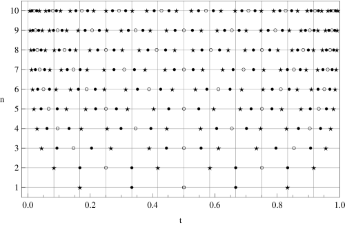
Figure 1: Switching times for orders $n=1$ to $n=10$. UDD switching times are open circles ○. Even permutation $A_{3}$ DFS DD switching times are filled circles ●only. Switching times for $S_{3}$ DFS DD over all six $S_{3}$ permutations include open circles, filled circles, and stars $\star$. The switching times are symmetric about $t=\frac{1}{2}$.

Table 2: $A_{3}$ DFS DD switching times corresponding to the filled circles in figure 1. Switching times listed are for the interval $[0,1]$. Only switching times less than $\frac{1}{2}$ are given explicitly. Switching times greater than $\frac{1}{2}$ are obtained by reflecting the given values about $t=\frac{1}{2}$.

• order $n$	$A_{3}$ switching times
  1	0.3333333333333333
  2	0.1666666666666667
  	0.3333333333333333
  3	0.0930802599812912
  	0.2041913710924023
  	0.4444444444444444
  4	0.0611678063574247
  	0.1320291453900112
  	0.2986958120566778
  	0.3945011396907580
  5	0.0422244245173296
  	0.0940587956886883
  	0.2172228408817372
  	0.2838895075484039
  	0.4518343711713587
  6	0.0313685011617312
  	0.0691609286752199
  	0.1617103538537611
  	0.2161866929592387
  	0.3514848584641742
  	0.4258827585118745
  7	0.0239219438795333
  	0.0535688803938237
  	0.1262566342290569
  	0.1675244212375237
  	0.2761133079137736
  	0.3417044666375784
  	0.4698392155798953

  order $n$	$A_{3}$ switching times
  8	0.0190156712850090
  	0.0422945303794296
  	0.1002297726086257
  	0.1346268067223472
  	0.2239571558152790
  	0.2763447583052162
  	0.3850761827426867
  	0.4416793537112741
  9	0.0153608717513108
  	0.0344809416081787
  	0.0820319124861268
  	0.1096019013513601
  	0.1835330371665574
  	0.2291713148467980
  	0.3223652733904291
  	0.3688693585992699
  	0.4721657549445159
  10	0.0127428989292003
  	0.0284688256262034
  	0.0679240161384205
  	0.0914464121824144
  	0.1538757061482468
  	0.1916101903303824
  	0.2714006848897883
  	0.3135792550438800
  	0.4050737288155140
  	0.4525790184049564

Filter functions corresponding to the Fourier transform of the two order $n$ $A_{3}$ switching functions $f_{1}^{(n)}(t)$ and $f_{2}^{(n)}(t)$ can be computed analogously to (10). Figure 2 shows the filter functions corresponding to the UDD switching function and the $A_{3}$ DFS DD switching functions for various orders of decoupling. Since all the switching functions of a given order are designed to integrate the same number of monomials to zero, they all exhibit the same low frequency filtering behavior.

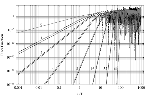
Figure 2: Filter functions for various decoupling orders. Dashed lines are the UDD filter functions. Black and gray lines are the $A_{3}$ DFS DD filter functions corresponding to $f_{1}^{(n)}(t)$ and $f_{2}^{(n)}(t)$, respectively. The sets of lines are labeled by their decoupling order $n$. $n=0$ is free evolution.

We have thus far restricted ourselves to decoupling over even permutations $A_{3}$ only. The previous considerations can be generalized to decoupling over all permutations of $S_{3}$. Defining the odd permutation Hamiltonian types as

$$H_{4}=Z_{2}B_{1}+Z_{1}B_{2}+Z_{3}B_{3},$$ (39)

$$H_{5}=Z_{3}B_{1}+Z_{2}B_{2}+Z_{1}B_{3},$$ (40)

$$H_{6}=Z_{1}B_{1}+Z_{3}B_{2}+Z_{2}B_{3},$$ (41)

and computing the accumulated phase difference integrals (cf. (34) – (35)) give rise to five sets of constraint equations (cf. (37) and (38)) and five independent $S_{3}$ switching functions. We find that a basic period 10 sequence of $\{H_{1},H_{4},H_{2},H_{5},H_{3},H_{6},H_{3},H_{5},H_{2},H_{4}\}$ allows order $n$ decoupling with $5n+1$ evolution intervals. The period 10 sequence alternates between even and odd permutations, with the transformation between successive Hamiltonians accomplished with a single swap gate on qubits 1 and 2, or qubits 2 and 3. The corresponding basic sequence of swap gates is $\{P_{1,2},P_{2,3},P_{1,2},P_{2,3},P_{1,2},P_{1,2},P_{2,3},P_{1,2},P_{2,3}\}$. As before, the final pulse in the sequence is chosen so that the pulses multiply to the identity. We can again solve the constraint equations numerically, and the switching times for $S_{3}$ DFS DD are also displayed in figure 1 (open circles ○, filled circles ●, and stars $\star$). The switching times for $S_{3}$ DFS DD are not unique. Because decoupling can be accomplished with even permutations alone, or with odd permutations alone, the relative weighting between even permutation decoupling and odd permutation decoupling is unconstrained. The switching times for $S_{3}$ DFS DD shown in figure 1 correspond to equal total time in even and odd permutations. Filter functions corresponding to the five $S_{3}$ switching functions may be computed according to (10). They have the same low-frequency roll-off behavior as the UDD filter function.

Table 3: $S_{3}$ DFS DD switching times corresponding to the stars in figure 1. Again, only switching times less than $\frac{1}{2}$ are given explicitly (see the caption to table 2). Full $S_{3}$ switching times include the values below, the values in table 2, and the UDD values (6).

• order $n$	$S_{3}$ switching times
  1	0.1666666666666667
  2	0.0833333333333333
  	0.4166666666666667
  3	0.0441757320558095
  	0.2663979542780318
  	0.3888888888888889
  4	0.0292438385042891
  	0.1706622892054447
  	0.2539956225387781
  	0.4459105051709558
  5	0.0198486448526978
  	0.1234090460471676
  	0.1855655208780249
  	0.3188988542113582
  	0.4035604011944698
  6	0.0148169093658703
  	0.0902375649702305
  	0.1365285435153074
  	0.2455460335064556
  	0.3140624574739186
  	0.4629576452117436
  7	0.0112075501170748
  	0.0704161635276064
  	0.1069644388480345
  	0.1894875256294779
  	0.2440254284265229
  	0.3752930054921819
  	0.4396659439243005

  order $n$	$S_{3}$ switching times
  8	0.0089377851765520
  	0.0553969487226799
  	0.0843798400197465
  	0.1531864662990289
  	0.1981928332289538
  	0.3030094142447375
  	0.3573598562810042
  	0.4706108187731435
  9	0.0071855182206674
  	0.0453635718581324
  	0.0692317973728011
  	0.1243583767250380
  	0.1614266670585074
  	0.2527437110834672
  	0.2994843851270477
  	0.3925059539229590
  	0.4443099124772396
  10	0.0059745260011464
  	0.0373611383696360
  	0.0571010082270104
  	0.1041446643790700
  	0.1355161859798696
  	0.2110062905707306
  	0.2508943643743651
  	0.3352721033248206
  	0.3812593890562080
  	0.4762946103276755

4 Decoupling the 3-qubit DFS from a quantum bath

A DFS qubit coupled to local quantum baths is described by the Hamiltonian

$$H=B_{0}+\vec{S}_{1}.\vec{B}_{1}+\vec{S}_{2}.\vec{B}_{2}+\vec{S}_{3}.\vec{B}_{3}.$$ (42)

Here $B_{0}$ is a pure bath operator describing interactions within the bath alone, and $\vec{B}_{j}=(B_{j,x},B_{j,y},B_{j,z})$ is a vector of bath operators coupled to constituent qubit $j$ through its Pauli operators $\vec{S}_{j}=(X_{j},Y_{j},Z_{j})$. As in section 3 full swaps are used to permute the qubits through the different bath operators. We define the quantum bath Hamiltonians analogously to (20), (22)–(23), and (39)–(41):

$$H_{1}=B_{0}+\vec{S}_{1}.\vec{B}_{1}+\vec{S}_{2}.\vec{B}_{2}+\vec{S}_{3}.\vec{B}_{3},$$ (43)

$$H_{2}=B_{0}+\vec{S}_{2}.\vec{B}_{1}+\vec{S}_{3}.\vec{B}_{2}+\vec{S}_{1}.\vec{B}_{3},$$ (44)

$$H_{3}=B_{0}+\vec{S}_{3}.\vec{B}_{1}+\vec{S}_{1}.\vec{B}_{2}+\vec{S}_{2}.\vec{B}_{3},$$ (45)

$$H_{4}=B_{0}+\vec{S}_{2}.\vec{B}_{1}+\vec{S}_{1}.\vec{B}_{2}+\vec{S}_{3}.\vec{B}_{3},$$ (46)

$$H_{5}=B_{0}+\vec{S}_{3}.\vec{B}_{1}+\vec{S}_{2}.\vec{B}_{2}+\vec{S}_{1}.\vec{B}_{3},$$ (47)

$$H_{6}=B_{0}+\vec{S}_{1}.\vec{B}_{1}+\vec{S}_{3}.\vec{B}_{2}+\vec{S}_{2}.\vec{B}_{3}.$$ (48)

The first and second order $A_{3}$ and $S_{3}$ DFS DD sequences for decoupling classical phase noise also decouple the DFS qubit from quantum baths. Consider the first order $A_{3}$ evolution sequence

$$P.\exp(-\rmi H\tau).P.\exp(-\rmi H\tau).P.\exp(-\rmi H\tau)$$ (49)

$$= \exp(-\rmi H_{3}\tau).\exp(-\rmi H_{2}\tau).\exp(-\rmi H_{1}\tau)$$ (50)

$$\approx 1-\rmi\tau\left(3B_{0}+\vec{S}_{\mathrm{tot}}.\vec{B}_{\mathrm{tot}}\right),$$ (51)

where

$$\vec{S}_{\mathrm{tot}}\equiv\vec{S}_{1}+\vec{S}_{2}+\vec{S}_{3},$$ (52)

$$\vec{B}_{\mathrm{tot}}\equiv\vec{B}_{1}+\vec{B}_{2}+\vec{B}_{3}.$$ (53)

The first order effective Hamiltonian contains only coupling to the total spin component operators of all three qubits. Similarly, the second order $A_{3}$ evolution sequence is

$$\exp(-\rmi H\tau).P^{-1}.\exp(-\rmi H\tau).P^{-1}.\exp(-2\rmi H\tau).P.\exp(-\rmi H\tau).P.\exp(-\rmi H\tau)$$ (54)

$$= \exp(-\rmi H_{1}\tau).\exp(-\rmi H_{2}\tau).\exp(-2\rmi H_{3}\tau).\exp(-\rmi H_{2}\tau).\exp(-\rmi H_{1}\tau)$$ (55)

$$\approx 1-2\rmi\tau\left(3B_{0}+\vec{S}_{\mathrm{tot}}.\vec{B}_{\mathrm{tot}}\right)-2\tau^{2}\left(3B_{0}+\vec{S}_{\mathrm{tot}}.\vec{B}_{\mathrm{tot}}\right)^{2}.$$ (56)

Again, the effective Hamiltonian depends to second order only on the total spin component operators. The first and second order $S_{3}$ DFS DD sequences can be expanded similarly and also decouple quantum baths.

For third and higher order, both the $A_{3}$ and $S_{3}$ sequences fail to decouple the quantum bath to the nominal order. To find higher order sequences for decoupling the quantum bath, we have resorted to brute force computational searches. We seek a sequence of Hamiltonians $H_{\sigma(k)}$ and associated time intervals $\tau_{k}$ such that the product of unitary propagators

$$U=\prod_{k=1}^{N}\exp(-\rmi H_{\sigma(k)}\tau_{k})$$ (57)

has an effective Hamiltonian that couples only to the total spin operators $S_{\mathrm{tot},x}$, $S_{\mathrm{tot},y}$, and $S_{\mathrm{tot},z}$, to the desired decoupling order. Here $N$ is the total number of evolution intervals and $\sigma(k)$ specifies under which Hamiltonian (43)–(48) interval $k$ evolves.

Given some candidate sequence of Hamiltonians, we expand (57) to the desired decoupling order in $\tau$. Because there are three qubits in the DFS, the system-bath interaction terms are at most weight three Pauli products on the system (constituent) qubits. The set of 64 Pauli products of weight three or less is partitioned into 16 equivalence classes under the action of the group $S_{3}$. For example, $X_{1}$ is in the equivalence class consisting of $[X_{1},X_{2},X_{3}]$, and $X_{1}Y_{2}$ is in the equivalence class consisting of $[X_{1}Y_{2},X_{1}Y_{3},Y_{1}X_{2},Y_{1}X_{3},X_{2}Y_{3},Y_{2}X_{3}]$. In the order-by-order expansion of (57) the coefficients of the Pauli products in the same equivalence class must be equal in order to achieve an effective Hamiltonian that couples to global interactions alone. Note that the coefficients consist of products of bath operators, with some numerical prefactor. Because the various bath operators do not commute, they further grade the terms that must be set equal. A candidate Hamiltonian sequence is a valid decoupling solution if $\tau_{k}$’s can be found such that members of each of the equivalence classes have the same coefficients, with the $\tau_{k}$’s real and positive. For the examples above, if the members of the $[X_{1}]_{S_{3}}$ equivalence class all couple to the bath operator $C$, the corresponding global interaction term is $S_{\mathrm{tot},x}.C$. Similarly, if the members of the $[X_{1}Y_{2}]_{S_{3}}$ equivalence class all couple to the bath operator $D$, the corresponding global interaction terms are $(S_{\mathrm{tot},x}S_{\mathrm{tot},y}-\rmi S_{\mathrm{tot},z}).D$.

With this methodology, we have found the third order quantum bath decoupling sequence shown in table 4. Rather than giving switching times, we have listed the evolution time intervals corresponding to a total evolution time of 1. The sequence consists of 26 Hamiltonian intervals, with a “doubly palindromic” structure. The first 13 Hamiltonians are all even permutations while the second 13 are all odd permutations. The second 13 Hamiltonian types can be determined from the first 13 via the mapping $H_{1}\rightarrow H_{4}$, $H_{2}\rightarrow H_{6}$, and $H_{3}\rightarrow H_{5}$. The interval timings for the odd permutations are identical to the even permutations. Within each set of 13 intervals, the interval timings are palindromic. Other length 26 third order solutions have been found, but the one displayed in table 4 is optimal in the sense that the ratio between the maximum and minimum interval lengths is smallest.

Table 4: Third order DFS decoupling sequence for a quantum bath, consisting of 26 Hamiltonian intervals. The first column lists the Hamiltonian type (43)–(48). The second column gives the interval length (rather than the switching times). The third column gives the pulse required at the end of the Hamiltonian interval. Only the first 13 intervals are given; the interval timings and pulses for the second 13 intervals are identical.

• Hamiltonian type	interval length	pulse
  $H_{1}$	0.02443154605193963	$P$
  $H_{2}$	0.03273388118971666	$P$
  $H_{3}$	0.05269740572865081	$P^{-1}$
  $H_{2}$	0.03073701555573789	$P^{-1}$
  $H_{1}$	0.04633548169315730	$P^{-1}$
  $H_{3}$	0.05049836419256131	$P$
  $H_{1}$	0.02513261117647280	$P$
  $H_{2}$	0.05049836419256131	$P^{-1}$
  $H_{1}$	0.04633548169315730	$P^{-1}$
  $H_{3}$	0.03073701555573789	$P^{-1}$
  $H_{2}$	0.05269740572865081	$P$
  $H_{3}$	0.03273388118971666	$P$
  $H_{1}$	0.02443154605193963	$P_{1,2}$

5 Numerical Simulations

Numerical simulations of a DFS qubit coupled to classical and quantum baths have been performed to illustrate the performance of the DFS decoupling sequences. Figure 3 shows a log-log plot of the infidelity versus total evolution time for a DFS qubit coupled to a classical dephasing only bath, with $A_{3}$ DFS DD sequences of orders $n=0$ to $n=4$ applied to the DFS qubit. The infidelity is defined as $1-F$, where $F$ is given by (31). The classical bath functions have size $|B_{j}(t)|\sim 100$MHz and $|(dB_{j}/dt)/B_{j}|\sim 100$MHz. Each point in figure 3 gives the infidelity after a single round of $n^{\mathrm{th}}$ order decoupling for the corresponding total evolution time $T$ on the abscissa; each point is averaged over 50 dephasing bath instances and 100 initial encoded DFS states. The plot markers correspond to $A_{3}$ DFS DD orders $n=0$ through $n=4$ as described in the figure caption. For $n^{\mathrm{th}}$ order decoupling, the phase differences (34)–(36) at short total times $T$ have dependence $\sim T^{n+1}$; the corresponding infidelity has total time dependence $\sim T^{2(n+1)}$. The dotted lines in figure 3 are fits to the function $a-bT^{2(n+1)}$ for each order of decoupling. At short total times the infidelity scales as expected, with a straight-line dependence on the log-log plot. The slopes of the fits have the predicted values of $2(n+1)$, indicating that the DFS DD sequences decouple the dephasing baths to their designed orders.

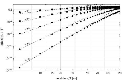
Figure 3: Simulations of a DFS qubit coupled to a classical dephasing-only bath. Infidelity is plotted against total evolution time $T$ for $A_{3}$ DFS DD orders $n=0$ (free evolution) through $n=4$. $n=0$ infidelities are given by ●, $n=1$ by ■, $n=2$ by $\blacklozenge$, $n=3$ by $\blacktriangle$, $n=4$ by $\blacktriangledown$. Dotted lines are fits to the given leading order infidelity term.

Figure 4 shows a log-log plot of infidelity versus total evolution time for a DFS qubit coupled to a quantum bath. We simulate a DFS qubit coupled to a bath composed of six spins; each constituent system qubit is coupled to two bath spins, and all six bath spins are coupled to each other. The Hamiltonian simulated is

$$H=J\left(\sum_{j=1}^{2}r_{1,j}\vec{S}_{1}.\vec{I}_{j}+\sum_{j=3}^{4}r_{2,j}\vec{S}_{2}.\vec{I}_{j}+\sum_{j=5}^{6}r_{3,j}\vec{S}_{3}.\vec{I}_{j}\right)+\beta\sum_{j=1}^{6}\sum_{k=j+1}^{6}r_{j,k}\vec{I}_{j}.\vec{I}_{k},$$ (58)

which has the same structure as (42). In (58) $J$ gives the energy scale of the system-bath coupling, $\beta$ gives the energy scale of the intra-bath coupling, $r_{i,j}$ are random numbers between 0 and 1, $\vec{S}_{j}$ is the vector of Pauli operators for the $j^{\mathrm{th}}$ system spin, and $\vec{I}_{j}$ is the vector of Pauli operators for the $j^{\mathrm{th}}$ bath spin. We take $J=100$MHz and $\beta=$10KHz for the simulations in figure 4. The simulations are “numerically exact” in that the propagators for full system and bath evolution are determined by computing the matrix exponential of the Hamiltonian (58); swaps between system qubits are interspersed between the propagators as required by the DFS DD protocols. Fidelities are again computed according to (31), with the states, propagator $U$, and projector $\Pi$ suitably generalized to include both the system and bath, and the addition of a partial trace operation over the bath spins. Each data point in figure 4 shows the infidelity computed for a given total evolution time, for decoupling orders $n=0$ through $n=3$. Each data point gives the infidelity averaged over 52 random initial conditions and Hamiltonians. The first and second order decoupling sequences used are $S_{3}$ DFS DD sequences; the third order sequence used is given in table 4. As in the classical bath case, the infidelity is expected to scale as $T^{2(n+1)}$. The dotted lines giving fits to the function $a-bT^{2(n+1)}$ confirm the expected scaling.

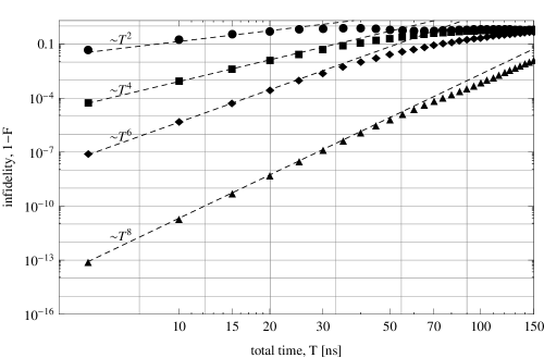
Figure 4: Simulations of a DFS qubit coupled to a quantum bath. Infidelity is plotted against total evolution time $T$ for DFS DD orders $n=0$ (free evolution) through $n=3$. $n=1$ and $n=2$ use $S_{3}$ DFS DD pulse sequences; $n=3$ uses the pulse sequence in table 4. $n=0$ infidelities are given by ●, $n=1$ by ■, $n=2$ by $\blacklozenge$, $n=3$ by $\blacktriangle$. Dotted lines are fits to the given leading order infidelity term.

6 Conclusion

We have shown that exchange pulses alone are sufficient to decouple the 3-qubit DFS from classical and quantum baths. By averaging over permutations of the 3 constituent qubits, local baths can be made to appear global to high order. Because the 3-qubit DFS is immune to global decoherence, DFS DD protects the encoded information. Numerical simulations of the new DFS decoupling pulse sequences confirm DD sequence performance expected from analytical considerations.

Decoupling of the 3-qubit DFS from classical and quantum baths may also be accomplished using NUDD (nested Uhrig dynamical decoupling) pulse sequences [10]. The DFS DD pulse sequences, however, are far more efficient. For example, for third order decoupling from a quantum bath, $n=3$, NUDD requires $(n+1)^{2\times 3}=4096$ pulse intervals, compared to 26 pulse intervals for the DFS decoupling described in section 4. Accounting for the structure of the DFS—protecting the encoded information only and using exchange pulses only—substantially reduces the number of pulses needed for decoupling and removes the need for single qubit Pauli gates. The fact that only a particular subspace or subsystem needs to be protected should be used in designing efficient decoupling pulse sequences for general qubit encodings.

Decoupling by averaging over the symmetric group (or one of its subgroups) using exchange pulses can be generalized to other decoherence free subspaces and subsystems [15]. The most efficient sequences as well as the types of errors protected against will depend on the encoding, the structure of the system-bath coupling, and the noise model. For the 2-qubit decoherence free subspace, for example, in which the encoding protects against collective decoherence in a single direction (say $z$), decoupling over $S_{2}$ protects against bath variations in the $z$ direction only. Bath variations in the $x$ and $y$ directions will cause leakage out of the encoded subspace. Decoupling over $S_{2}$ has exactly the same structure as UDD for a single qubit: a full swap on the exchange gate between the two qubits takes the role of the Pauli $X$ pulse for the single qubit, and the interval timings are the UDD timings (6). For other encodings protecting against weak collective decoherence [15], averaging over $S_{n}$ subgroups will decouple bath variations in the encoding-protected direction only. For encodings protecting against strong collective decoherence (which includes the 3-qubit DFS) averaging over $S_{n}$ subgroups decouples the encoded information from all bath components. The effective global interaction created by the averaging affects only the gauge while leaving the encoded information unchanged. The quantum numbers describing encoded states correspond to total spin operators on increasing numbers of the constituent qubits, and all total spin operators commute with global interactions. Determination of switching times and pulse interval Hamiltonian types for decoupling other DFS encodings can be found by generalizing the methods described in this paper.

Finally, we note that the correspondence between $S_{2}$ decoupling and UDD of a 2-level system, each coupled to classical dephasing bath(s) along a single direction, generalizes to a correspondence between decoupling a $d$-qubit DFS and a $d$-level system ($SU(d)$) from classical dephasing baths along a single direction [24]. In these cases averaging over the $d$ cyclic permutations of the system for the DFS or cyclic permutations of the $d$ levels yields the same pulse interval Hamiltonian types and switching times.

Appendix

For an initial encoded state $\left|\psi_{e}\right\rangle=(r,\sqrt{1-r^{2}}e^{\rmi\phi})$, the coefficients in the fidelity expression (32) are

$$c_{0} = \frac{1}{6}\left(3-2r^{2}+2r^{4}+2r^{2}(1-r^{2})\cos 2\phi\right),$$ (59)

$$c_{1} = \frac{2}{9}(1-r^{2})\left(1+2r^{2}+2r\sqrt{3(1-r^{2})}\cos\phi\right),$$ (60)

$$c_{2} = \frac{2}{9}(1-r^{2})\left(1+2r^{2}-2r\sqrt{3(1-r^{2})}\cos\phi\right),$$ (61)

$$c_{3} = \frac{1}{18}\left(1-2r^{2}+10r^{4}-6r^{2}(1-r^{2})\cos 2\phi\right).$$ (62)

References

References

- [1] E. L. Hahn. Spin echoes. Physical Review, 80(4):580–594, November 1950.
- [2] H. Y. Carr and E. M. Purcell. Effects of diffusion on free precession in nuclear magnetic resonance experiments. Physical Review, 94(3):630–638, May 1954.
- [3] S. Meiboom and D. Gill. Modified spin-echo method for measuring nuclear relaxation times. Review of Scientific Instruments, 29:688–691, 1958.
- [4] Götz S. Uhrig. Keeping a quantum bit alive by optimized -pulse sequences. Physical Review Letters, 98:100504, 2007.
- [5] Götz S. Uhrig. Exact results on dynamical decoupling by pulses in quantum information processes. New Journal of Physics, 10:083024, 2008.
- [6] Wen Yang and Ren-Bao Liu. Universality of Uhrig dynamical decoupling for suppressing qubit pure dephasing and relaxation. Physical Review Letters, 101:180403, 2008.
- [7] Michael J. Biercuk, Hermann Uys, Aaron P. VanDevender, Nobuyasu Shiga, Wayne M. Itano, and John J. Bollinger. Optimized dynamical decoupling in a model quantum memory. Nature, 458:996–1000, 2009.
- [8] Hermann Uys, Michael J. Biercuk, and John J. Bollinger. Optimized noise filtration through dynamical decoupling. Physical Review Letters, 103:040501, 2009.
- [9] Jacob R. West, Bryan H. Fong, and Daniel A. Lidar. Near-optimal dynamical decoupling of a qubit. Physical Review Letters, 104:130501, April 2010.
- [10] Zhen-Yu Wang and Ren-Bao Liu. Protection of quantum systems by nested dynamical decoupling. Physical Review A, 83:022306, 2011.
- [11] J.R. Petta, A.C. Johnson, J.M. Taylor, E.A. Laird, A. Yacoby, M.D. Lukin, C.M. Marcus, M.P. Hanson, and A.C. Gossard. Coherent manipulation of coupled electron spins in semiconductor quantum dots. Science, 309(5744):2180–2184, September 2005.
- [12] F.H.L. Koppens, C. Buizert, K.J. Tielrooij, I.T. Vink, K.C. Nowack, T. Meunier, L.P. Kouwenhoven, and L.M.K. Vandersypen. Driven coherent oscillations of a single electron spin in a quantum dot. Nature, 442:766–771, August 2006.
- [13] K.C. Nowack, F.H.L. Koppens, Yu.V. Nazarov, and L.M.K. Vandersypen. Coherent control of a single electron spin with electric fields. Science, 318:1430–1433, November 2007.
- [14] D. Bacon, J. Kempe, D.A. Lidar, and K.B. Whaley. Universal fault-tolerant quantum computation on decoherence-free subspaces. Physical Review Letters, 85(8):1758–1761, August 2000.
- [15] J. Kempe, D. Bacon, D.A. Lidar, and K.B. Whaley. Theory of decoherence-free fault-tolerant universal quantum computation. Physical Review A, 63(042307), March 2001.
- [16] J. Kempe, D. Bacon, D.P. DiVincenzo, and K.B. Whaley. Encoded universality from a single physical interaction. Quantum Information and Computation, 1:33–55, 2001.
- [17] D.P. DiVincenzo, D. Bacon, J. Kempe, G. Burkard, and K.B. Whaley. Universal quantum computation with the exchange interaction. Nature, 408:339–342, November 2000.
- [18] B.H. Fong and S.M. Wandzura. Universal quantum computation and leakage reduction in the 3-qubit decoherence free subsystem. Quantum Information and Computation, 11(11&12):1003–1008, November 2011.
- [19] L.-A. Wu and D.A. Lidar. Creating decoherence-free subspaces using strong and fast pulses. Physical Review Letters, 88(20):207902, 2002.
- [20] L.-A. Wu, M.S. Byrd, and D.A. Lidar. Efficient universal leakage elimination for physical and encoded qubits. Physical Review Letters, 89(12):127901, 2002.
- [21] Mark S. Byrd, Daniel A. Lidar, Lian-Ao Wu, and Paolo Zanardi. Universal leakage elimination. Physical Review A, 71:052301, 2005.
- [22] Łukasz Cywiński, Roman M. Lutchyn, Cody P. Nave, and S. Das Sarma. How to enhance dephasing time in superconducting qubits. Physical Review B, 77:174509, 2008.
- [23] M. J. Biercuk, A. C. Doherty, and H. Uys. Dynamical decoupling sequence construction as a filter-design problem. Journal of Physics B: Atomic, Molecular and Optical Physics, 44:154002, 2011.
- [24] Sujeet Shukla, Liang Jiang, John Preskill, and Adilet Imambekov. Generalized Uhrig dynamical decoupling for multi-level quantum systems. In http://meetings.aps.org/Meeting/MAR12/Event/159721, 2012.