Cosmic-ray Electron Evolution in the Supernova Remnant RX J1713.7-3946 

Abstract

A simple formalism to describe nonthermal electron acceleration, evolution, and radiation in supernova remnants (SNRs) is presented. The electron continuity equation is analytically solved assuming that the nonthermal electron injection power is proportional to the rate at which the kinetic energy of matter swept up in an adiabatically expanding SNR shell. We apply this model to Fermi and HESS data from the SNR RX J1713.7-3946, and find that a one-zone leptonic model with Compton-scattered cosmic microwave background (CMB) and interstellar infrared photons has difficulty providing a good fit to its spectral energy distribution, provided the source is at a distance $\sim 1\ \mathrm{kpc}$ from the Earth. However, the inclusion of multiple zones, as hinted at by recent Chandra observations, does provide a good fit, but requires a second zone of compact knots with magnetic fields $B\sim 16\ \mu$G, comparable to shock-compressed fields found in the bulk of the remnant.

1. Introduction

Acceleration of particles at SNR shocks is considered the leading mechanism for the production of cosmic-ray protons and ions from energies of $\approx 1$ GeV/nucleon up to the knee of the cosmic-ray spectrum (e.g., Lagage & Cesarsky, 1983; Blandford & Eichler, 1987; Berezinskii et al., 1990). As the expanding SNR shell sweeps up matter from the surrounding circumstellar medium (CSM), a pair of shocks is formed, with the leading forward shock sweeping up and accelerating CSM material, and a reverse shock braking the metal-rich SNR ejecta. A few select particles gain energy as they randomly diffuse back and forth across each of the two shock fronts, while convecting downstream into the shocked fluid. In the test particle theory of first-order Fermi acceleration, this leads to a nonthermal power-law particle distribution in momentum with number spectral near $-2$ for a compression ratio near 4. The spectrum that results after folding in the effects of diffusive escape from the SNR into intergalactic space, and from the disk of the Galaxy into the halo, is in reasonable agreement with the measured cosmic-ray spectrum (e.g., Jones & Ellison, 1991; Kirk, 1994; Hillas, 2005).

Charged cosmic rays are deflected by Galactic magnetic fields during transport, so their direction does not point back to the original production site. This is the principal reason that the sources of Galactic cosmic rays remain elusive a century after their discovery. Given the extreme difficulty in detecting neutrinos (Yuan et al., 2011b), electromagnetic signatures of cosmic rays offer at present the best opportunity to identify the sources of cosmic rays and settle the question of their origin (e.g., Ginzburg & Syrovatskii, 1964; Gaisser, 1990; Drury et al., 1994; Reynolds, 2008).

With speeds reaching $10^{4}$ km s^-1 or more, SNR shocks are likely candidates for accelerating electrons and nucleons to high energies. The polarization and spectral properties of the smooth broadband nonthermal radio through X-ray emission is almost certainly electron synchrotron radiation, though the optical, UV and X-ray spectra can additionally reveal strong line signatures from shock-heated shell material (Slane et al., 2002; Badenes et al., 2006). Several radiative mechanisms can be responsible for $\gamma$-ray emission. Energetic leptons emit $\gamma$ rays through Compton scattering of the ambient radiation fields, principally the cosmic microwave background (CMB) and ambient stellar and IR fields, but also by scattering photons of the the synchrotron field. Electrons make nonthermal bremsstrahlung $\gamma$ rays when colliding with target gas and dust particles in the circumstellar medium (CSM) or in the shocked shell material. Nuclear collisions of hadrons make pion-decay $\gamma$ rays when cosmic-ray protons and ion interact with that same matter. Spectral and morphological differences are expected between a leptonic and hadronic origin. Most well known is the prediction of the $\pi^{0}$ decay feature peaking at 70 MeV in a photon spectrum (Ginzburg & Syrovatskii, 1964; Hayakawa, 1969) that results from hadronic processes. For an electron injection spectrum softer than number index $q=2$ (where the injected electrons are injected with spectrum $Q(\gamma)\propto\gamma^{-q}$), as expected in the test-particle limit for strong nonrelativistic shocks in a hydrogen medium, the Compton-scattered radiation spectrum is much harder than the electron bremsstrahlung $\gamma$-ray spectrum. For a consistent explanation, the synchrotron spectrum must also be compatible with the same electron distribution that makes the $\gamma$ rays.

Differences between morphological features can help discriminate between leptonic and hadronic origins of $\gamma$ rays in SNRs. Emission of $\gamma$ rays from bremsstrahlung and proton interactions is expected to be enhanced in the vicinity of dense molecular clouds, not only due to the denser target material, but also due to the increased amount of energy dissipated at the shock front (e.g., Bykov et al., 2000; Aharonian & Atoyan, 1996; Gabici et al., 2009). Almost all SNRs associated with Fermi sources exhibit OH maser emission from SNR/molecular cloud interactions (Hewitt et al., 2009). By contrast, synchrotron X-rays and TeV $\gamma$-rays from Compton-scattered CMB photons require only high-energy electrons and a magnetic field, and in principle could be found in regions of small gas density.

Recent Fermi Large Area Telescope (LAT) observations have provided a wealth of data on SNRs. The First Fermi Catalog of Gamma Ray Sources (1FGL; Abdo et al., 2010a) lists 41 associations with sources in Green’s SNR catalog (Green, 2009). Morphological similarities allow definite identifications to be made in 3 cases: 1FGL J1856.1+0122 with W44 (Abdo et al., 2010b); 1FGL J1922.9+1411 with W51C (Abdo et al., 2009); and 1FGL J0617.2+2233 with IC 443 (Abdo et al., 2010c). In the second Fermi-LAT catalog (2FGL; Abdo et al., 2011a), 3 additional SNR identifications are reported besides a total of 62 associations with SNRs and pulsar wind nebulae. More recently, RX J1713.7-3946 has been added to this list (Abdo et al., 2011b). The Fermi data provide strong evidence that $\gamma$-ray emission is made by accelerated particles in the vicinity of these objects. Yet it is not conclusive that the SNRs are accelerating the particles, as pre-existing cosmic rays compressed by the outflowing remnant could make the emission (Uchiyama et al., 2010).

There have been numerous hadronic and leptonic models produced to explain the particle acceleration and $\gamma$-ray emission from SNRs, with varying degrees of complexity (e.g., Sturner et al., 1997; Baring et al., 1999; Zirakashvili & Aharonian, 2007; Lee et al., 2008). Here we focus on a simple model for electron acceleration at the forward SNR shock and study the evolving distribution with the addition of radiative and adiabatic losses (however, note that acceleration in the reverse shock could be substantial; Telezhinsky et al., 2012). The goal is to explain the RX J1713.7-3946 spectrum with a purely leptonic model involving Compton scattering of diffuse target photons and a possible small contribution from electron bremsstrahlung. As the SNR expands into the CSM and decelerates due to the addition of the swept-up matter, the particle injection power initially increases in the free-expansion phase, and subsequently declines in the Sedov phase. The time-dependent injection efficiency is very model dependent, and ultimately rests on microphysical plasma processes. Here we normalize the power of injected nonthermal electrons to the swept-up power; other normalizations could employ an injection efficiency proportional to the rate at which particle mass is swept up, or an efficiency dependent on shock speed and compression ratio.

In Section 2 we describe our model. In Section 3, we use it to fit the multiwavelength SED of the SNR RX J1713.7-3946 (G 347.3$-$0.5), and show that a single-zone model is incapable of fitting the spectrum. A model with a second zone of emission regions consisting of compact knots is shown to give a good fit to the SED. We conclude with a summary and discussion in Section 4.

2. Formalism

We make a number of common simplifying assumptions. A spherically-symmetric supernova explosion finds itself in a homogeneous surrounding CSM with constant number density $n_{CSM}$. The explosion is approximated by an expanding shell of matter that sweeps up CSM material. The inclusion of the swept-up mass controls the dynamics of the shell, and the system proceeds to channel directed kinetic energy into internal kinetic energy of the shocked matter. The injection rate changes abruptly at the Sedov age. We purposely keep the transition between the pre-Sedov (i.e., free expansion) and Sedov phases discrete to highlight interesting injection effects, keeping in mind that a more detailed treatment would have a smooth pre-Sedov and post-Sedov transition.

2.1. SNR Dynamics

Here we describe a simple formalism for the dynamics of SNRs. A detailed hydrodynamic description is given by Truelove & McKee (1999). The kinetic energy, $E$, of the remnant and swept up matter is conserved in an adiabatic blast wave, so that

$$E=\frac{1}{2}M_{0}v_{0}^{2}=\frac{1}{2}\left[M_{0}+\frac{4\pi}{3}m_{p}n_{CSM}r(t)^{3}\right]v^{2}(t)\ ,$$ (1)

where $M_{0}$ and $v_{0}$ are the initial remnant’s mass and speed, respectively, $m_{p}$ is the proton mass, and $r(t)$ and $v(t)=dr/dt$ are respectively the radius and speed of the SNR as a function of time $t$. For simplicity, the CSM is assumed to be composed entirely of hydrogen. The Sedov radius, $r_{s}$, is defined as the radius where the mass of the swept-up CSM matter, $4\pi m_{p}n_{CSM}r(t)^{3}/3$, is equal to the mass of the initial explosion, $M_{0}$, i.e.,

$$r_{s}\equiv\left[\frac{3M_{0}}{4\pi m_{p}n_{CSM}}\right]^{1/3}\ .$$ (2)

Using Equation (2), Equation (1) can be rewritten

$$v_{0}^{2}=\left[1+\left(\frac{r}{r_{s}}\right)^{3}\right]\left(\frac{dr}{dt}\right)^{2}\ ,$$ (3)

or

$$v(t)=\frac{dr}{dt}=\frac{v_{0}}{\left[1+(r/r_{s})^{3}\right]^{1/2}}\ .$$ (4)

This can be solved in the limit $r\ll r_{s}$ , giving

$$r(t)=v_{0}t\ ,$$ (5)

which is known as the free expansion phase of the remnant. In the Sedov phase, $r\gg r_{s}$, giving the well-known behavior

$$r(t)=v_{0}t_{s}\left(\frac{5t}{2t_{s}}\right)^{2/5}\ .$$ (6)

Here the Sedov time is defined as

$$t_{s}\equiv\frac{r_{s}}{v_{0}}\ .$$ (7)

The solutions (5) and (6) intersect when $t=1.84t_{s}$. The speed of the remnant in these limits is

$$v(t)=\left\{\begin{array}[]{ll}v_{0}&r\ll r_{s}\\ v_{0}\left(5t/2t_{s}\right)^{-3/5}&r\gg r_{s}\end{array}\right.\ .$$ (8)

The solutions for $r\ll r_{s}$ and $r\gg r_{s}$ intersect when $t=0.40t_{s}$. The rate at which kinetic energy is swept up from the surrounding CSM is

$$\frac{dE}{dt}=2\pi r^{2}n_{CSM}m_{p}v^{3}\ .$$ (9)

In Figure 1 we plot the radius and speed of the remnant for the exact expression, Equation (4), and the approximate expressions, Equations (5), (6), and (8). As can be seen, the approximate form reproduces the exact behavior quite well.

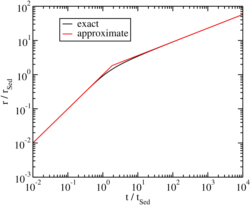
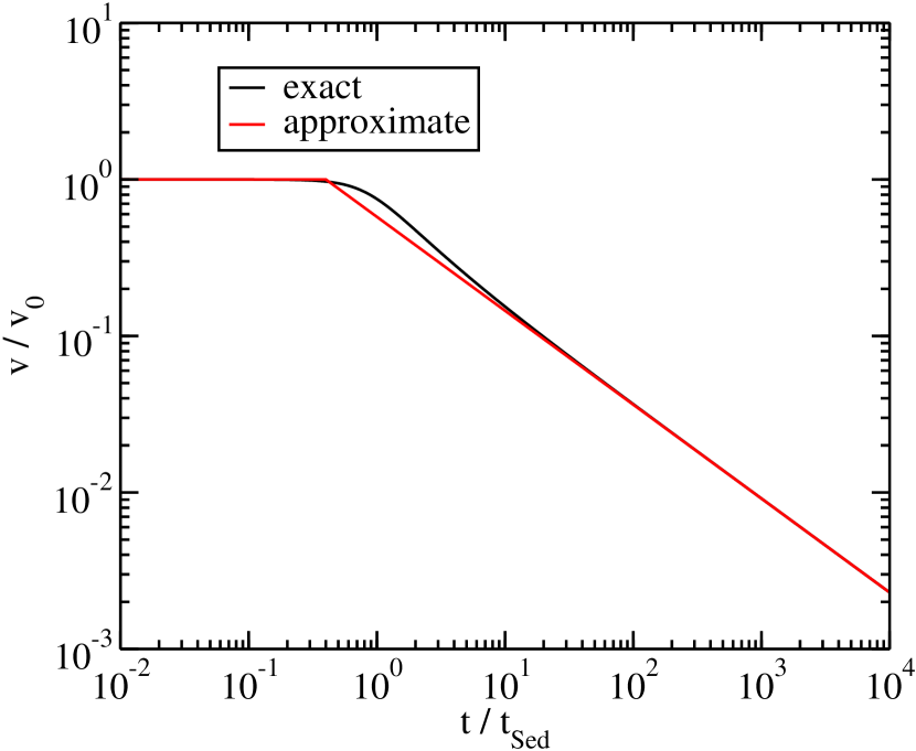
Figure 1.— Evolution of SNR radius and speed using the exact and approximate expressions.

2.2. Particle Acceleration

As the SNR shock expands into the CSM, particles will be accelerated at the forward shock, to which we restrict our treatment. We assume that the injected kinetic energy of the nonthermal particle distribution is some fraction $\eta$ of the swept-up kinetic energy. This energy is swept into the shocked fluid and allows us to normalize the the nonthermal injection function, $Q(\gamma,t)$ by the relation

$$mc^{2}\int^{\gamma_{2}}_{\gamma_{1}}d\gamma\ \gamma\ Q(\gamma,t)=\eta 2\pi r^{2}n_{CSM}m_{p}v^{3}\ ,$$ (10)

where $\gamma$ is the particle’s Lorentz factor and $m$ is the particle’s mass. In order not to sweep in more energy than was originally available, $\eta$ is restricted to be $\ll 1$, and the treatment is restricted to an adiabatic blast wave.

Assuming that the injected accelerated particle distribution function can be described by a power law, then

$$Q(\gamma,t)=Q_{0}(t)\ \gamma^{-q}H(\gamma;\gamma_{1},\gamma_{2})\ ,$$ (11)

where $H(x;a,b)=1$ if $a\leq x\leq b$, and $H(x;a,b)=0$ otherwise. Equation (10) can be integrated to give

$$Q_{0}(t)=\frac{r^{2}v^{3}\ 2\pi n_{CSM}m_{p}\ \eta}{mc^{2}}$$

$$\times\left\{\begin{array}[]{ll}(q-2)(\gamma_{1}^{2-q}-\gamma_{2}^{2-q})^{-1}&{\rm for~{}}q\neq 2\\ \\ \left[\ln(\gamma_{2}/\gamma_{1})\right]^{-1}&{\rm for~{}}q=2\end{array}\right.\ .$$ (15)

Equation (4) can be inserted into Equation (15) and used to write an approximate expression for $Q(\gamma,t)$,

$$Q(\gamma,t)=Kf(t)\gamma^{-q}$$ (16)

where

$$K\equiv\frac{v_{0}^{5}t_{s}^{2}\ 2\pi n_{CSM}m_{p}\ \eta}{mc^{2}}$$

$$\times\left\{\begin{array}[]{ll}(q-2)(\gamma_{1}^{2-q}-\gamma_{2}^{2-q})^{-1}&q\neq 2\\ \left[\ln(\gamma_{2}/\gamma_{1})\right]^{-1}&q=2\end{array}\right.\$$ (17)

and

$$f(t)=\frac{(r/r_{s})^{2}}{\left[1+(r/r_{s})^{3}\right]^{3/2}}\ .$$ (18)

The approximation

$$f(t)\approx\left\{\begin{array}[]{ll}(t/t_{s})^{2}&t<Ct_{s}\\ (5t/2t_{s})^{-1}&t>Ct_{s}\end{array}\right.\ .$$ (19)

is in accord with the asymptotes for $r(t)$ and $v(t)$ from Section 2.1. The division of the two branches of the approximation at $Ct_{s}$ where $C\approx 0.74$ was chosen to produce a continuous function. The exact expression for $f(t)$, Equation (18) is compared with the approximation from Equation (19) in Figure 2. As can be seen, the approximation is quite good, with small discrepancies around $t\approx t_{s}$.

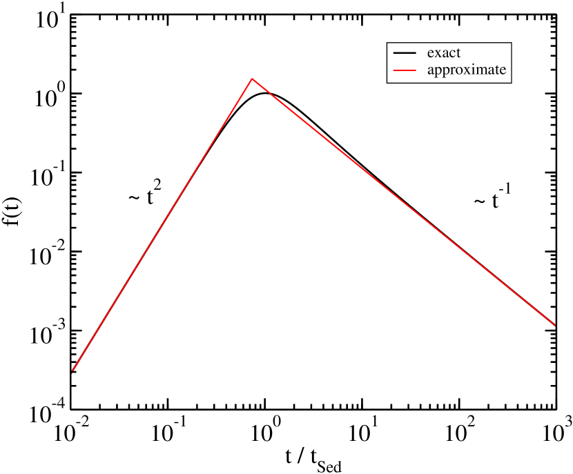
Figure 2.— The exact (Equation [18]) and approximate (Equation [19]) expressions for $f(t)$.

Using the power in the swept-up CSM to normalize the rate of particle acceleration, as described above, is also standard for GRBs (e.g., Chiang & Dermer, 1999) but differs from what has been done in the past for SNRs. Earlier normalizations related the number of accelerated electrons to the number of electrons swept into the expanding blast wave (e.g., Sturner et al., 1997; Reynolds, 1998; Baring et al., 1999), which leads to a considerably different time-dependence in the Sedov phase for the accelerated electrons ($Q(\gamma,t)\propto t^{1/5}$ instead of $Q(\gamma,t)\propto t^{-1}$).

The maximum particle energy can be calculated by equating the acceleration time with the radiative loss time or the age of the remnant (Reynolds, 1998). To keep the treatment analytic, here we assume $\gamma_{max}$ is constant in time.

2.3. Particle Evolution

When $Q(\gamma,t)$ has been determined (Section 2.2), the evolution of the particle distribution, $N(\gamma;t)$ can be found by solving the continuity equation,

$$\frac{\partial N}{\partial t}+\frac{\partial}{\partial\gamma}\left[\dot{\gamma}\ N(\gamma;t)\right]+\frac{N(\gamma;t)}{t_{esc}(\gamma,t)}=Q(\gamma,t)\ ,$$ (20)

where $t_{esc}$ is the escape timescale and $\dot{\gamma}$ is the cooling rate. Analytic solutions to the particle continuity equation (20) are discussed in Kardashev (1962); Blumenthal & Gould (1970); and Dermer & Menon (2009, Appendix C).

2.3.1 Solution with Radiative Losses

For electrons, escape timescales can be long and hence will be neglected. The electron Lorentz factor $\bar{\gamma}$ above which synchrotron losses dominate bremsstrahlung losses is $\bar{\gamma}\approx 5\times 10^{4}\ (n_{CSM}/{\rm cm}^{-3})(10\ \mu{\rm G}/B)^{2}$, but the corresponding timescale for energy loss is $\approx 5\times 10^{7}$ yrs. This is much longer than the age of the remnant even for very dense target material, so bremsstrahlung losses can be safely neglected. Thus we assume electron energy losses are dominated by radiative losses from synchrotron and Thomson scattering of CMB photons, so that

$$-\dot{\gamma}=\nu\ \gamma^{2}$$ (21)

where

$$\nu=\frac{4c\sigma_{\rm T}[B^{2}/(8\pi)+u_{CMB}]}{3m_{e}c^{2}}\$$ (22)

$$=1.34\times 10^{-20}~{}{\rm s}^{-1}[1+(B/3.23\ {\mu}\mathrm{G})^{2}]\;,$$

$B$ is the magnetic field in the remnant, and $u_{CMB}=4.13\times 10^{-13}\ \mathrm{erg}\ \mathrm{cm}^{-3}$ is the energy density of the CMB at the present epoch. Klein-Nishina effects should be of little importance to the evolution of the electron spectrum as long as the synchrotron losses dominate over Compton losses, which will be the case for $B\gtrsim 3\ \mu\mathrm{G}$. In this situation, the continuity equation has the solution

$$\gamma^{2}N_{e}(\gamma;t)=K\int_{t_{min}}^{t}\ dt_{i}\ \gamma_{i}^{2-q}\ f(t_{i})\$$ (23)

(see Appendix A; also Kardashev, 1962; Blumenthal & Gould, 1970; Dermer, 1998). Here

$$\gamma_{i}=\frac{1}{\gamma^{-1}-\nu(t-t_{i})}\ ,$$ (24)

and

$$t_{min}=\max[0,t-\nu^{-1}(\gamma^{-1}-\gamma_{2}^{-1})]\ .$$ (25)

It is instructive to look at the case $q=2$, where the integral in Equation (23) can be performed analytically. For $t<Ct_{s}$,

$$\gamma^{2}N_{e}(\gamma;t)=\frac{Kt_{s}}{3}\left[\left(\frac{t}{t_{s}}\right)^{3}-\left(\frac{t_{min}}{t_{s}}\right)^{3}\right]\ ,$$ (26)

while for $t>Ct_{s}$ and $t_{min}<Ct_{s}$,

$$\gamma^{2}N_{e}(\gamma;t)=Kt_{s}\left[\frac{1}{3}\left(C^{3}-\left(\frac{t_{min}}{t_{s}}\right)^{3}\right)+\frac{2}{5}\ln\left(\frac{t}{Ct_{s}}\right)\right]\ .$$ (27)

For $t>Ct_{s}$ and $t_{min}>Ct_{s}$,

$$\gamma^{2}N_{e}(\gamma;t)=\frac{2Kt_{s}}{5}\ln\left(\frac{t}{t_{min}}\right)\ .$$ (28)

Now we examine the asymptotes for this solution, starting with the case where $t<Ct_{s}$. In the limit $t\ll(\nu\gamma)^{-1}$ or $\gamma\ll(\nu t)^{-1}$, $t_{min}\rightarrow 0$, and

$$\gamma^{2}N_{e}(\gamma;t)\approx K\ \frac{t^{3}}{3t_{s}^{2}}\propto t^{3}\ \gamma^{0}\ .$$ (29)

For $t\gg(\nu\gamma)^{-1}$ or $\gamma\gg(\nu t)^{-1}$,

$$\gamma^{2}N_{e}(\gamma;t)\approx\frac{K}{3\nu\gamma}\left(\frac{t}{t_{s}}\right)^{2}\ \propto t^{2}\gamma^{-1}.$$ (30)

Thus, at low $\gamma$ ($\gamma\ll(\nu t)^{-1}$), the electron distribution will have the power-law injection index (i.e., $N_{e}(\gamma;t)\propto\gamma^{-q}$), and at high $\gamma$ ($\gamma\gg(\nu t)^{-1}$), the electron distribution will be $N_{e}(\gamma;t)\propto\gamma^{-q+1}$, as seen in Equations (29) and (30) and as expected for a cooling distribution. Since the electron distribution increases at different rates in the different regimes, however, an inflection will open up in the normalization of the distribution in these two regimes.

This effect becomes more pronounced for $t>Ct_{s}$. In this case, if $\gamma\ll(\nu t)^{-1}$,

$$\gamma^{2}N_{e}(\gamma;t)\approx Kt_{s}\left[\frac{1}{3}+\frac{2}{5}\ln\left(\frac{t}{Ct_{s}}\right)\right]\propto\gamma^{0}\ \ln(t/Ct_{s})\ .$$ (31)

For $\gamma\gg(\nu t)^{-1}$ and $\gamma>\nu^{-1}(t-t_{s})^{-1}$,

$$\gamma^{2}N_{e}(\gamma;t)\approx\frac{Kt_{s}}{\nu\gamma t}\propto t^{-1}\ \gamma^{-1}\ .$$ (32)

Thus, at low $\gamma$ ($\gamma\ll(\nu t)^{-1}$), the electron distribution will again have the same power-law index with as the injection term, just as with $t<Ct_{s}$, and the overall normalization will increase with time, although more slowly than at $t<Ct_{s}$. At large $\gamma$, the electron distribution will be $N_{e}(\gamma;t)\propto\gamma^{-q+1}$, but the normalization will be decreasing with time. This will lead to an increasingly large gap in normalization of the cooled ($\gamma<(\nu t)^{-1}$) and uncooled ($\gamma>(\nu t)^{-1}$) electrons as time increases. This behavior can be seen in Fig. 3. Similar behavior can be found for $q\neq 2$, as demonstrated in Fig. 4, where the integral in Equation (23) is performed numerically. The parameters used in these calculations can be found in Table 1.

Table 1 Test model parameters.

Parameter	Symbol	Model
Blast Energy [erg]	$E$	$1.0\times 10^{51}$
Initial Mass [$M_{\odot}$]	$M_{0}$	1.6
Initial Velocity [$\mathrm{cm}\ \mathrm{s}^{-1}$]	$v_{0}$	$8.0\times 10^{8}$
ICM density [$\mathrm{cm}^{-3}$]	$n_{ICM}$	1.0
Sedov time [yr]	$t_{s}$	303
Magnetic field [$\mu$G]	$B$	10
Cooling Constant [$\mathrm{s}^{-1}$]	$\nu$	$1.4\times 10^{-19}$
Low energy electron cutoff	$\gamma_{1}$	10
High energy electron cutoff	$\gamma_{2}$	$3.1\times 10^{9}$
Electron acceleration efficiency	$\eta_{e}$	$10^{-4}$

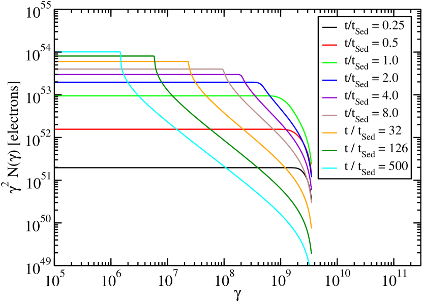
Figure 3.— Evolution of electron distribution with radiative losses only for $q=2$. Parameters are given in Table 1.

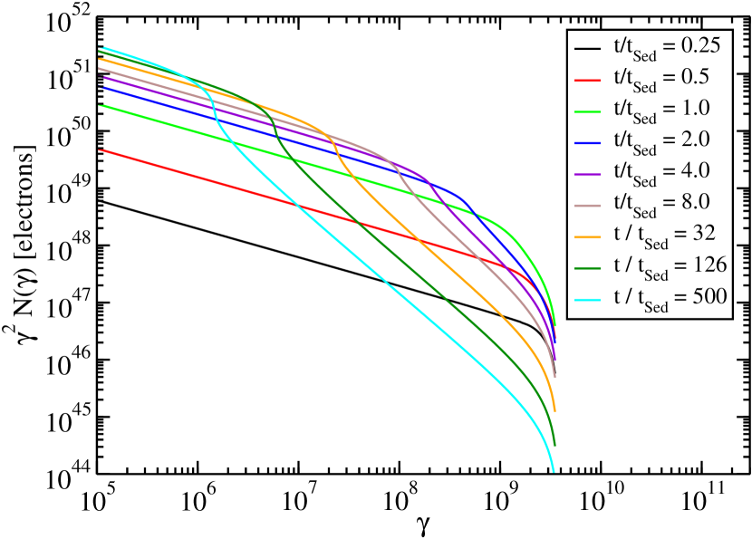
Figure 4.— Same as Figure 3 for $q=2.5$. Parameters are given in Table 1.

2.3.2 Solution with Adiabatic Losses

As the remnant expands, particles lose energy due to adiabatic losses, since they are trapped in the expanding SNR. The loss rate from this process is

$$-\dot{\gamma}=\frac{\gamma}{3}\frac{dV}{dt}\frac{1}{V}=\frac{k_{ad}\gamma}{t}$$ (33)

(e.g., Gould, 1975) where the remnant’s volume is $V\propto r(t)^{3}$. Details of the expansion control the adiabatic coefficient $k_{ad}$, and in principle one can imagine a shell that contracts in width while expanding outward to give no volume change, so $k_{ad}\rightarrow 0$ for this peculiar system (see, e.g. Truelove & McKee, 1999, for a hydrodynamic description). In our approximations, $k_{ad}=1$ for $r\ll r_{s}$, and $k_{ad}=2/5$ for $r\gg r_{s}$, given $r(t)$ and $v(t)$ from Equations (5), (6), and (8). The results are only weakly dependent on the value of $k_{ad}$, and so here we will assume the same $k_{ad}$ in both regimes, eventually taking $k_{ad}=1$ for simplicity. See Reynolds (2008) for a discussion on the dependence of the shock radius with time for core collapse and type Ia progenitors, which has implications for $k_{ad}$.

If adiabatic cooling dominates and radiative cooling is negligible, then the solution to the continuity Equation gives

$$N(\gamma;t)=Kt\int^{t}_{t_{min}}\frac{dt_{i}}{t_{i}}\ \left(\frac{\gamma t^{k_{ad}}}{t_{i}^{k_{ad}}}\right)^{-q}f(t_{i})$$ (34)

where

$$t_{min}=\left(\frac{\gamma}{\gamma_{2}}\right)^{1/k_{ad}}t\ .$$ (35)

The integral can be performed analytically. If $t<Ct_{s}$,

$$N(\gamma;t)=\frac{Kt^{3}\gamma^{-q}}{t_{s}^{2}(qk_{ad}+2)}\left[1-\left(\frac{\gamma}{\gamma_{2}}\right)^{qk_{ad}+2}\right]\ .$$ (36)

If $t>Ct_{s}$ and $\gamma t/\gamma_{2}<t_{s}$,

$$N(\gamma;t)=K\gamma^{-q}$$

$$\times\Biggr{[}\frac{t^{3}}{t_{s}^{2}(qk_{ad}+2)}\left(\left(\frac{Ct_{s}}{t}\right)^{qk_{ad}+2}-\left(\frac{\gamma}{\gamma_{2}}\right)^{(qk_{ad}+2)/k_{ad}}\right)$$

$$+\frac{2t_{s}}{5(qk_{ad}-1)}\left(1-\left(\frac{Ct_{s}}{t}\right)^{qk_{ad}-1}\right)\Biggr{]}\ .$$ (37)

If $t>t_{s}$ and $\gamma t/\gamma_{2}>t_{s}$,

$$N(\gamma;t)=\frac{2K\gamma^{-q}t_{s}}{5(qk_{ad}-1)}\left[1-\left(\frac{\gamma}{\gamma_{2}}\right)^{(qk_{ad}-1)/k_{ad}}\right]\ .$$ (38)

2.3.3 Solution with Radiative and Adiabatic Losses

If adiabatic and cooling losses are important, then the cooling rate will have the form

$$-\dot{\gamma}=\nu\ \gamma^{2}+k_{ad}\frac{\gamma}{t}\ .$$ (39)

In this case, if $k_{ad}=1$, the continuity Equation has the solution (see Appendix B)

$$\gamma^{2}N(\gamma;t)=\frac{K}{t}\int^{t}_{t_{min}}dt_{i}\ t_{i}\ \gamma_{i}^{2-q}\ f(t_{i})$$ (40)

where

$$\gamma_{i}=\left[t_{i}\left((\gamma t)^{-1}-\nu\ln(t/t_{i})\right)\right]^{-1}\ ,$$ (41)

$$t_{min}=\left[W\left(\frac{1}{\gamma_{2}\nu t}e^{1/(\gamma\nu t)}\right)\gamma_{2}\ \nu\right]^{-1}\ ,$$ (42)

and $W(x)$ is the Lambert $W$ function, defined by

$$x=W(x)e^{W(x)}\$$ (43)

(e.g., Corless et al., 1996). The integral can be done analytically if $q=2$. In this case, for $t<t_{s}$,

$$\gamma^{2}N(\gamma;t)=\frac{K}{4\ t\ t_{s}^{2}}\left(t^{4}-t_{min}^{4}\right)\ .$$ (44)

For $t>Ct_{s}$ and $t_{min}<Ct_{s}$,

$$\gamma^{2}N(\gamma;t)=\frac{K}{t}\left[\frac{1}{4t_{s}^{2}}((Ct_{s})^{4}-t_{min}^{4})+\frac{2t_{s}}{5}\left(t-Ct_{s}\right)\right]\ .$$ (45)

For $t>Ct_{s}$ and $t_{min}>Ct_{s}$,

$$\gamma^{2}N(\gamma;t)=\frac{2Kt_{s}}{5t}\left(t-t_{min}\right)\ .$$ (46)

The asymptotes of this solution can also be found. We begin with the case of $t<Ct_{s}$. For $t\ll(\nu\gamma)^{-1}$ or $\gamma\ll(\nu t)^{-1}$, the argument in the Lambert function in Equation (42) goes to infinity, so the Lambert function goes to infinity, and $t_{min}\rightarrow 0$. Then,

$$\gamma^{2}N(\gamma;t)\approx\frac{Kt^{3}}{4t_{s}^{2}}\propto\ t^{3}\ \gamma^{0}\ .$$ (47)

For $t\gg(\nu\gamma)^{-1}$ or $\gamma\gg(\nu t)^{-1}$, a Taylor expansion of the exponential and Lambert function in Equation (42) gives $t_{min}\rightarrow t-(\nu\gamma)^{-1}$. Then

$$\gamma^{2}N(\gamma;t)\approx\frac{Kt^{2}}{16t_{s}^{2}\nu\gamma}\propto t^{2}\gamma^{-1}\ .$$ (48)

These results are quite similar to the asymptotes for the radiative-only case (Section 2.3.1). The results for $t>Ct_{s}$ are, however, somewhat different. In this case, for $t\ll(\nu\gamma)^{-1}$ or $\gamma\ll(\nu t)^{-1}$,

$$\gamma^{2}N(\gamma;t)\approx Kt_{s}\left[\frac{2}{5}-\frac{3t_{s}}{20t}\right]\ \approx\frac{2Kt_{s}}{5}\propto t^{0}\gamma^{0}\ .$$ (49)

For $t\gg(\nu\gamma)^{-1}$ or $\gamma\gg(\nu t)^{-1}$,

$$\gamma^{2}N(\gamma;t)\approx\frac{2Kt_{s}}{5\nu t\gamma}\ \propto t^{-1}\gamma^{-1}\ .$$ (50)

Here, the behavior for large $\gamma$ is essentially the same as the radiative-only case. However, the addition of adiabatic losses means that the electrons at low $\gamma$ will approach a constant value, rather than increasing logarithmically without bound. This will remove the inflection seen in the radiative-only case. An example of this can be seen in Figure 5, where it is clear the inflection in the radiative losses-only solution (Section 2.3.1) is not seen. Results are very similar for other values of $k_{ad}$, particularly $k_{ad}=0.4$, as one would expect in the Sedov phase.

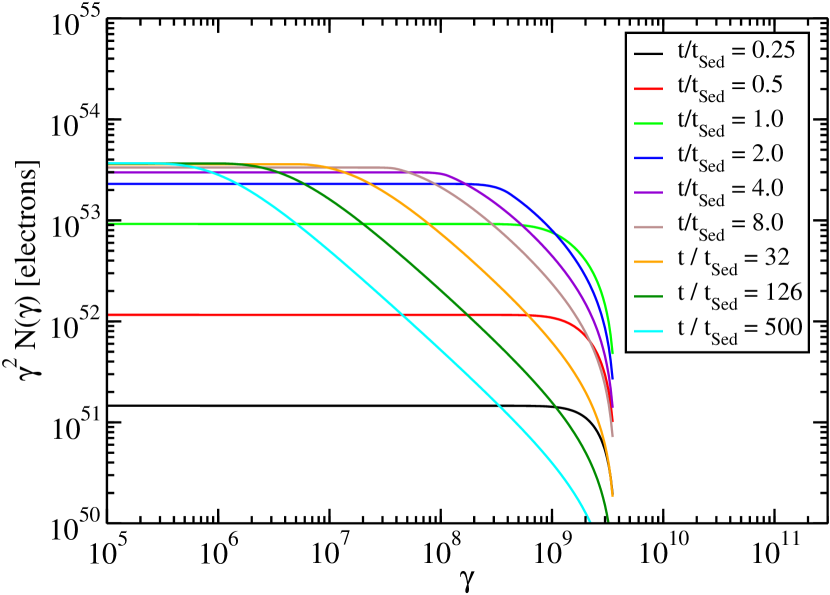
Figure 5.— Evolution of electron distribution for q=2 including adiabatic and radiative cooling. Parameters are given in Table 1.

2.4. Spectral Energy Distribution

Once the electron distribution has been determined, as above, the spectral energy distribution (SED) from the SNR can be calculated. For electrons in a randomly-oriented magnetic field $B$, the $\nu F_{\nu}$ synchrotron flux, $f_{\epsilon}^{syn}$ is given by

$$f_{\epsilon}^{syn}=\frac{\sqrt{3}\epsilon e^{3}B}{4\pi hd^{2}}\int^{\infty}_{1}d\gamma\ N_{e}(\gamma;t)\ R(x)\ ,$$ (51)

where $e=4.8\times 10^{-10}$ esu is the elementary charge, $\epsilon=h\nu/(m_{e}c^{2})$ is the dimensionless observed photon energy, $h=6.63\times 10^{-27}\ \mathrm{erg}$-s is Planck’s constant, $d$ is the distance to the SNR,

$$x=\frac{4\pi m_{e}^{2}c^{3}}{3eBh\gamma^{2}}\ ,$$ (52)

$$R(x)=\frac{x}{2}\int_{0}^{\pi}d\theta\ \sin\theta\ \int^{\infty}_{x/\sin\theta}dt\ K_{5/3}(t)\$$ (53)

(Crusius & Schlickeiser, 1986), and $K_{5/3}(t)$ is the modified Bessel function of order 5/3. Approximate expressions for $R(x)$ are given by Zirakashvili & Aharonian (2007); Finke, Dermer, & Böttcher (2008); and Joshi & Böttcher (2011).

The electrons will also Compton-scatter external photon sources, such as the CMB or other intergalactic sources. The flux from external Compton (EC) scattering a blackbody photon source with total energy density $u_{tot}$ and dimensionless temperature $\Theta=k_{B}T/(m_{e}c^{2})$ is given by

$$f_{\epsilon}^{EC}=\frac{3m_{e}c\sigma_{\rm T}\epsilon^{2}}{16\pi d^{2}}\frac{15u_{tot}}{(\pi\Theta)^{4}}$$ (54)

$$\times\int_{0}^{\infty}d\epsilon_{*}\ \frac{\epsilon_{*}}{\exp(\epsilon_{*}/\Theta)-1}$$

$$\times\int_{\gamma_{min}}^{\gamma_{max}}d\gamma\ \gamma^{-2}\ N_{e}(\gamma;t)\ F_{C}(\epsilon,\gamma,\epsilon_{*})$$

where $\sigma_{\rm T}=6.65\times 10^{-25}\ \mathrm{cm}^{2}$ is the Thomson cross section. For the CMB at the present epoch, $\Theta=4.58\times 10^{-10}$ and $u_{tot}=4.2\times 10^{-13}\ \mathrm{erg}\ \mathrm{cm}^{-3}$ are the dimensionless CMB temperature and energy density at the present epoch. The integration limits are given by

$$\gamma_{min}=\frac{1}{2}\epsilon\left(1+\sqrt{1+\frac{1}{\epsilon_{*}\epsilon}}\right)\ ,$$ (55)

$$\gamma_{max}=\frac{\epsilon_{*}\epsilon}{\epsilon_{*}-\epsilon}H(\epsilon_{*}-\epsilon)\ ,$$ (56)

and the function

$$F_{C}(\epsilon,\gamma,\epsilon_{*})=\biggr{[}2q\ln q+(1+2q)(1-q)+{1\over 2}{(\Gamma_{e}q)^{2}\over(1+\Gamma_{e}q)}(1-q)\biggr{]}$$

$$\times H\;\left(q;{1\over 4\gamma^{2}},1\right)\ ,$$ (57)

where

$$q\equiv{\epsilon/\gamma\over\Gamma_{e}(1-\epsilon/\gamma)}\;\;{\rm,~{}and}\;\;\Gamma_{e}=4\epsilon_{*}\gamma\;$$ (58)

(Jones, 1968; Blumenthal & Gould, 1970). The electrons can also Compton-scatter the synchrotron photons produced by the same electron population (known as synchrotron self-Compton or SSC), which is given by

$$f_{\epsilon}^{SSC}=\frac{9}{16}\frac{\sigma_{\rm T}\epsilon^{2}}{\pi r^{2}}$$

$$\times\int^{\infty}_{0}\ d\epsilon_{*}\ \frac{f_{\epsilon_{*}}^{syn}}{\epsilon_{*}^{3}}\ \int^{\gamma_{max}}_{\gamma_{min}}\ d\gamma\ \frac{N_{e}(\gamma)}{\gamma^{2}}F_{C}(q,\Gamma)\$$ (59)

(e.g., Finke et al., 2008). This mechanism is usually negligible for large, diffuse remnants, but will play a roll in Section 3.2.

The nonthermal electrons from the remnant will interact with the cold ions (assumed to be protons) in the surrounding CSM to make bremsstrahlung (or free-free radiation) with flux given by

$$f_{\epsilon}^{ff}=\frac{n_{CSM}m_{e}c^{3}\epsilon^{2}}{4\pi d^{2}}$$

$$\times\int_{1}^{\infty}\ d\gamma\ N_{e}(\gamma;t)\ \frac{d\sigma_{ff,eZ}}{d\epsilon}(\epsilon;\gamma)\ ,$$ (60)

where the bremsstrahlung cross section is written as

$$\frac{d\sigma_{ff,eZ}}{d\epsilon}(\epsilon;\gamma)=$$

$$\frac{4Z^{2}\alpha_{f}r_{e}^{2}}{\epsilon}\left(1+y-\frac{2y}{3}\right)\left[\ln\left(\frac{2\gamma^{2}y}{\epsilon}\right)-\frac{1}{2}\right]$$ (61)

(Blumenthal & Gould, 1970), $Z$ is the effective charge of the cold ions, $\alpha_{f}\approx(137)^{-1}$ is the fine structure constant, $r_{e}=2.82\times 10^{-13}\ \mathrm{cm}$ is the classical electron radius, and $y=1-\epsilon/\gamma$.

The synchrotron and Compton emission can be seen in Figs. 6 and 7, corresponding to the respective electron distributions seen in Figs. 3 and 5. These SEDs assume emission from an SNR at $d=1\ \mathrm{kpc}$. In the Sedov phase, the feature resulting from the different evolution above and below the cooling break is clearly seen for the case when adiabatic losses are neglected (Figure 6), but this feature is not as pronounced when adiabatic losses are taken into account (Figure 7).

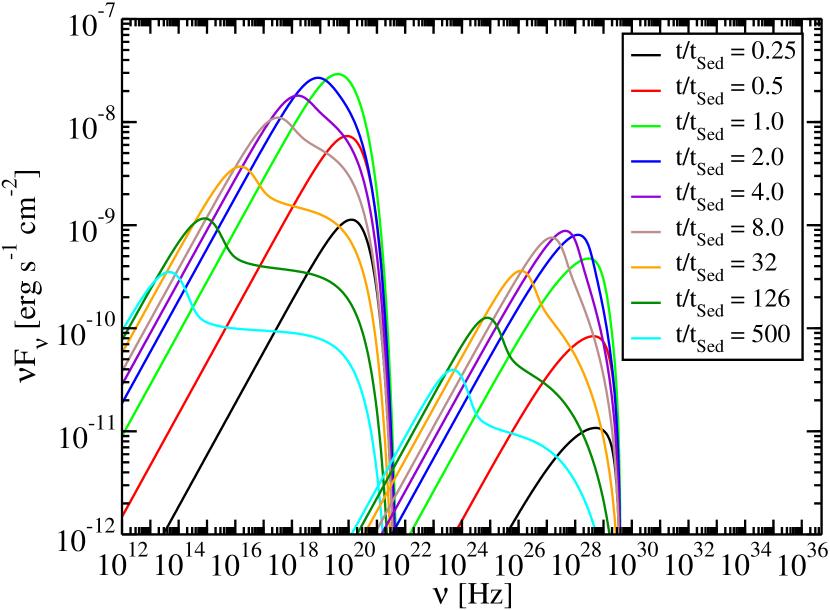
Figure 6.— Evolution of synchrotron and Compton-scattered CMB flux for the electron distribution in Figure 3.

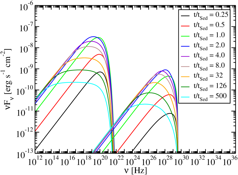
Figure 7.— Evolution of synchrotron and Compton-scattered CMB flux for the electron distribution in Figure 5.

3. Application to the Remnant RX J1713.7-3946

We apply our results to SNR RX J1713.7-3946 (G 347.3$-$0.5), which is thought to be the remnant of a “guest star” observed by Chinese astronomers in 393 CE (Wang et al., 1997). This fixes it age at $\cong 1620$ yr, so SNR RX J1713.7-3946 is likely to be well into the Sedov phase, although Fukui et al. (2003) argue instead that it is still in the free expansion stage, for CSM densities $n_{CSM}<0.01$ cm^-3 at $\approx 1$ kpc distance. Slane et al. (1999) associated the source with a nearby molecular cloud, giving a distance to the source of $\sim 6\ \mathrm{kpc}$. However, newer CO observations found molecular gas at $\sim 1\ \mathrm{kpc}$, (Fukui et al., 2003; Moriguchi et al., 2005). Absorbing column densities from X-ray observations strengthen the $\sim 1\ \mathrm{kpc}$ distance estimate (Koo et al., 2004; Cassam-Chenaï et al., 2004), making it the most likely one. The detection of an X-ray point source, thought to be a left-over neutron star, implies the remnant is the result of a core-collapse supernova (Lazendic et al., 2003).

The X-ray spectrum of RX J1713.7-3946 appears completely dominated by nonthermal emission (e.g., Tanaka et al., 2008). The lack of thermal X-ray lines is taken as evidence that $n_{CSM}\lesssim 0.2\ \mathrm{cm}^{-3}$ (Slane et al., 1999; Ellison et al., 2010; Abdo et al., 2011b). Without a dense target for cosmic ray protons, $\pi^{0}$ decay is probably not a significant contributor to the $\gamma$-ray spectrum of this remnant (Ellison et al., 2010), and electron bremsstrahlung is weak in comparison with the Compton $\gamma$-ray emission. But note the different energy ranges of electrons that radiate into the $\gamma$-ray band: electrons with Lorentz factor $\gamma\sim 10^{6}$ ($\sim 10^{8}$) scatter CMB photons to GeV (10 TeV) ranges, and electrons with $\gamma\sim 10^{3}$ ($\sim 10^{6}$) make GeV (TeV) bremsstrahlung.

HESS observations show that the X-ray image of RX J1713.7-3946 and the VHE $\gamma$-rays are spatially well-correlated (Aharonian et al., 2004, 2006). Uchiyama et al. (2007) reported X-ray variability on a year timescale in a few small (arcsecond scale) hotspots of RX J1713.7-3946. If this reflects radiative variability of the nonthermal electrons, large magnetic fields are needed ($B\sim 1$ mG), and the implied small number of electrons in such a strong magnetic field could not produce the TeV emission. But the appearance of thin radio-emitting rims in some SNRs could mean that the emission zone is compact and variability is due to shell expansion or compression as it encounters dilute or dense CSM (Reynolds, 2010; Reynolds et al., 2011). Furthermore, the existence of knots which do not seem to be variable on such short timescales indicates knots may exist with significantly lower magnetic fields. Based on the HESS observations, Aharonian et al. (2006) concluded that a leptonic model was unlikely to fit the broadband SED, and a hadronic origin was favored for the $\gamma$ rays from RX J1713.7-3946. The variable X-ray filaments cannot, however, explain global TeV emission (Butt et al., 2008).

With the arrival of the first epoch Fermi data from RX J1713.7-3946 (Abdo et al., 2011b), different models can be tested better. This seems to make it a good time to revisit leptonic models, which are natural for RX J1713.7-3946 given the close spatial correlation between the X-ray and TeV $\gamma$ rays.

3.1. Single Zone Model Fit

The integrated broadband SED of RX J1713.7-3946 is shown in Fig. 8. Porter et al. (2006) have shown that the interstellar infrared radiation field (IIRF) can be a significant photon source for Compton scattering. It is strongly dependent on the position in the Galaxy, and close to the Galactic center their model (Moskalenko et al., 2006) gives the IIRF energy density greater than that of the CMB. At a Galactic longitude of $\ell=347.3\arcdeg$ and a Galactic latitude of $b=-0.5\arcdeg$, this remnant is nearly along the line of sight of the Galactic center. This makes the intensity of the IIRF strongly dependent on its distance from the Earth (and therefore the Galactic center). The consensus, based on associations of molecular clouds and absorption of X-rays (as discussed above, in Section 3) seems to be that the RX J1713.7-3946is at $d=1\ \mathrm{kpc}$ from Earth. Therefore in our modeling we use this distance, and an IIRF intensity consistent with this distance (or $7.5\ \mathrm{kpc}$ from the Galactic center) from Porter et al. (2006), modeled as a blackbody with temperature $T=30\ \mathrm{K}$ and total energy density $u=4.8\times 10^{-13}\ \mathrm{erg}\ \mathrm{cm}^{-3}=0.30\ \mathrm{eV}\ \mathrm{cm}^{-3}$. Note that Li et al. (2011) modeled the source using the IIRF at a level near what one would expect (Porter et al., 2006) if RX J1713.7-3946 was $d=6\ \mathrm{kpc}$ from the Earth.

The models in Figure 8 include adiabatic and radiative losses from both the CMB and IIRF, and apply to the integrated emission over the entire remnant. In our modeling we have added this radiation field as an additional term in equation (22) to take it into account in the evolution of the SNR. We take the age of the remnant to be $t=1620\ \mathrm{yr}$. A best fit to the SED, given reasonable parameter constraints on age, ICM density, initial mass, and blast energy, is shown in the figure as the black curve. This model includes emission from synchrotron, Compton-scattering of CMB and IIRF photons, and bremsstrahlung, which can be seen as a small bump at $\sim 10^{21}\ \mathrm{Hz}$. It provides a good fit to the radio and X-ray data, but does not adequately reproduce the LAT and lower-energy HESS measurements.

The model parameters are shown in Table 2. The parameters which are constrained by the SED fit are $B$, $q$, $\gamma_{2}$, and $\eta_{e}$. We also display in this Figure models with 5 times larger and small $B$. As the magnetic field increases, the overall synchrotron flux increases, and the cooling electron Lorentz factor $(\nu t)^{-1}$ decreases. The magnetic field will only affect the Compton-scattered emission through its effects on the electron distribution; thus the overall Compton-scattered flux will not increase, and indeed will decrease above the the cooling break, which is lower for higher $B$.

Table 2 RX J1713.7-3946 Model Parameters

Parameter	Symbol	Model 1 (baseline)	Model 2	Model 3	Model 4	Model 5
Blast Energy [erg]	$E$	$1.6\times 10^{51}$	$1.6\times 10^{51}$	$1.6\times 10^{51}$	$1.6\times 10^{51}$	$1.6\times 10^{51}$
Initial Mass [$M_{\odot}$]	$M_{0}$	1.6	1.6	1.6	6.4	0.4
Initial Velocity [$\mathrm{cm}\ \mathrm{s}^{-1}$]	$v_{0}$	$1.0\times 10^{9}$	$1.0\times 10^{9}$	$1.0\times 10^{9}$	$5\times 10^{8}$	$2.0\times 10^{9}$
ICM density [$\mathrm{cm}^{-3}$]	$n_{ICM}$	0.2	0.2	0.2	0.2	0.2
Sedov time [yr]	$t_{s}$	420	420	420	1300	132
Magnetic field [$\mu$G]	$B$	12	60	2.4	12	12
Cooling Constant [$\mathrm{s}^{-1}$]	$\nu$	$2.2\times 10^{-19}$	$4.7\times 10^{-18}$	$3.7\times 10^{-20}$	$2.2\times 10^{-19}$	$2.2\times 10^{-19}$
Cooling electron Lorentz factor	$(\nu t)^{-1}$	$9.1\times 10^{7}$	$4.2\times 10^{6}$	$5.4\times 10^{8}$	$9.1\times 10^{7}$	$9.1\times 10^{7}$
Low energy electron cutoff	$\gamma_{1}$	10	10	10	10	10
High energy electron cutoff	$\gamma_{2}$	$3.1\times 10^{8}$	$3.1\times 10^{8}$	$3.1\times 10^{8}$	$3.1\times 10^{8}$	$3.1\times 10^{8}$
Injection spectral index	$q$	$2.1$	$2.1$	$2.1$	$2.1$	$2.1$
Electron acceleration efficiency	$\eta_{e}$	$5.0\times 10^{-5}$	$5.0\times 10^{-5}$	$5.0\times 10^{-5}$	$5.0\times 10^{-5}$	$5.0\times 10^{-5}$

In Fig. 9 we explore variations in $v_{0}$, which also correspond to variations in $M_{0}$, assuming $E$ is held constant, as given in Equation (1). The Sedov radius $r_{s}\propto v_{0}^{-2/3}$ as given in Equation (2), and thus $t_{s}\propto v_{0}^{-5/3}$ (Equation [7]) and $K\propto v_{0}^{5/3}$ (Equation [17]). Keeping this in mind, $t>t_{s}$ so that below the cooling break, $N_{e}(\gamma;t)\propto 1/3+(5/2)\ln(v_{0}^{5/3})$ from Equation (31) and above the break, $N_{e}(\gamma;t)\propto v_{0}^{0}$ (Equation [32]). This is reflected in the SED, as seen in Fig. 9, where below the break the emission increases with $v_{0}$, while above the break, the emission is independent of $v_{0}$. Also note that it is unlikely for the initial ejecta mass to be as low as found in Model 4, demonstrating the limited usefulness in varying $v_{0}$ to obtain a good fit to RX J1713.7-3946.

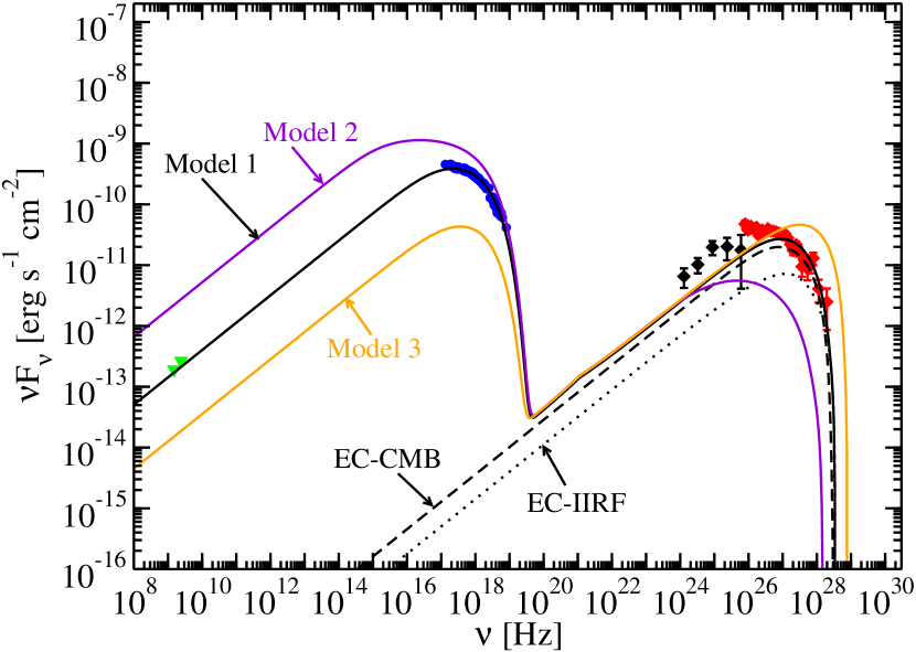
Figure 8.— The integrated broadband SED of RX J1713.7-3946 with data from ATCA (green triangles; Aharonian et al., 2006), Suzaku (blue circles; Tanaka et al., 2008), LAT (black diamonds; Abdo et al., 2011b), and HESS (red diamonds; Aharonian et al., 2006, 2007). The solid curves show the model fits for different magnetic fields, as labeled. The dashed and dotted curves show the Compton-scattered CMB and IIRF components, respectively, for Model 1.

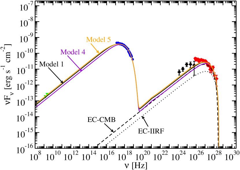
Figure 9.— Similar to Fig. 8, only $v_{0}$ is varied instead of $B$.

3.2. Multi-Zone model

As discussed above in Section 3, the discovery of variable X-ray filaments (or knots) within the SNR structure by Uchiyama et al. (2007) indicates that the single-zone fit is inadequate to explain the overall SED. However, the filaments themselves could contribute a significant amount to the $\gamma$-ray emission from the source.

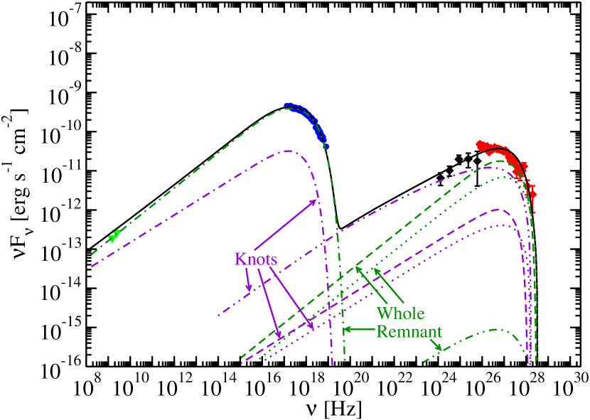
Figure 10.— Multi-zone model fit to RX J1713.7-3946. Curves show the total emission from the knots and overall shock combined (black solid curve) as well as synchrotron emission (dot-dashed curves), Compton-scattered CMB (dashed curves), Compton-scattered IIRF (dotted curves), and SSC (double dot-dashed curves) from the overall shock and knots.

Smaller knots emitting synchrotron, SSC, and Comptonized CMB and IIRF radiation were added to Model 1, as seen in Figure 10. The much smaller volume of these knots results in large synchrotron energy densities in the knots, with strong SSC emission at GeV energies. This fit has the number of zones taken to be $N_{knots}=100$, with each zone having $B_{knots}=16\ \mu$G, radii $R_{knot}=1\$mpc, and an electron distribution that spans from $\gamma_{knot,1}=10$ to $\gamma_{knot,2}=1.4\times 10^{8}$ with a break at $\gamma_{knot,brk}=4.7\times 10^{7}$ with $N_{e,knot}(\gamma)\propto\gamma^{-2.3}$ for $\gamma<\gamma_{knot,brk}$ and $N_{e,knot}(\gamma)\propto\gamma^{-3.3}$ for $\gamma>\gamma_{knot,brk}$. As can be seen in Figure 10, this reproduces the SED well, and makes interesting predictions.

The synchrotron component is dominated by the large first zone that effectively represents the entire remnant, which also makes the bulk of the TeV radiation. Emission $\gtrsim 1\ \mathrm{TeV}$ is dominated by the Compton-scattered CMB of the remnant as a whole, while in the range in the joint LAT/HESS window from $\lesssim 1\ \mathrm{TeV}$ the $\gamma$ rays arise from the SSC component in the knots. The angular resolution of the LAT is generally worse than $0.1\arcdeg$. At a distance of 1 kpc, the 1 mpc knots will have an angular radius of $0.2\arcsec$ and thus cannot be resolved with the LAT. CTA will have an angular resolution of $\sim 1\arcmin$ (CTA Consortium, 2010) and will not be able to distinguish the variable and non-variable X-ray knots seen by Uchiyama et al. (2007) either, even if they radiate in $\gamma$ rays. However, if the low and high energy $\gamma$-rays come from different components, maps of RX J1713.7-3946 made with CTA may be different at lower ($\lesssim 1\ \mathrm{TeV}$) and higher ($\gtrsim 1\ \mathrm{TeV}$) energies, with the higher energy maps being more in agreement with X-ray ones. This may allow this multi-zone model to be tested.

The knots contribute $\sim 10$% to the X-ray emission of the remnant, consistent with observations from Uchiyama et al. (2003). They are also much lower than the values inferred from variability by Uchiyama et al. (2007). However, there seem to be many knots which are not variable, which could reflect a lower magnetic field.

4. Discussion and Conclusions

The SNR RX J1713.7-3946 occupies an important place in $\gamma$-ray studies of supernova remnants. TeV emission from the SNR RX J1713.7-3946 was first detected with the CANGAROO experiment (Muraishi et al., 2000). Based on further CANGAROO observations, Enomoto et al. (2002) claimed that a standard leptonic synchrotron/EC-CMB model did not fit these data, including the EGRET upper limit. Reimer & Pohl (2002) argued that EGRET upper limits rule out a hadronic origin, but diffusion of high-energy particles upstream of the shock can harden nuclear emission (Malkov & Diamond, 2006). Aharonian et al. (2004) produced the first resolved $\gamma$-ray image of an SNR by HESS. Further HESS observations found that the X-ray and VHE $\gamma$-rays were spatially well-correlated (Aharonian et al., 2006). Porter et al. (2006) found, however, that Compton-scattered Galactic background photons, in addition to CMB photons, could help to explain the RX J1713.7-3946 VHE emission in leptonic models. Still further HESS observations detected the remnant out to $\sim 100~{}\mathrm{TeV}$ (Aharonian et al., 2007). Li et al. (2011) provide a good fit to the full SED including the LAT spectrum with a model similar to Porter et al. (2006), including Compton-scattering of interstellar infrared photons. As discussed above in Section 3.1, they assumed the source was at a distance of 6 kpc from us, closer to the Galactic center where the IIRF is much more intense. However, we think the molecular cloud and X-ray absorption evidence points to RX J1713.7-3946 most likely being at $d=1\ \mathrm{kpc}$. This emphasizes the crucial importance of an accurate distance measurement to SNR modeling.

New data from Fermi (Abdo et al., 2011b), in addition to multiwavelength measurements at radio, X-ray, and TeV energies, reveal the bolometric SED of SNR RX J1713.7-3946 with unprecedented detail. The joint Fermi-LAT/HESS data favor models (Porter et al., 2006; Berezhko & Völk, 2006; Ellison et al., 2010; Zirakashvili & Aharonian, 2010) where the $\gamma$ rays have a leptonic rather than a hadronic origin. This conclusion follows rather forcefully if the injection spectral index of the particles—protons or electrons—is softer than $q=2$, as expected in the linear first-order Fermi acceleration theory. Nonlinear effects may modify the injection index (e.g., Blasi et al., 2005). Indeed, Yamazaki et al. (2009) point out that nonlinear effects could harden the emission in the LAT energy range, making it nearly impossible to distinguish between leptonic and hadronic origins. Inoue et al. (2011) find that hard $\gamma$-ray spectra can be generated from $\pi^{0}$ decay if the CSM has inhomogeneities and is “clumpy”.

These results also test the conclusions of Fukui et al. (2011) based on a comparison of the TeV and CO and H I morphology. They interpreted the good correlation between the two bands as being a strong signature for a hadronic origin of the $\gamma$ rays, since cosmic ray protons would react with the molecular cloud hadrons. That interpretation is not unique to hadrons, however, as shocks in molecular clouds would enhance electron acceleration and leptonic $\gamma$-ray emission. Observations with HAWC and CTA, and longer exposures with the Fermi-LAT, will show the fraction of radiation from clumps at different energies, and will help clarify the issue. Here we consider broadband spectral modeling by following electron injection and evolution.

The complicated CSM distribution in any realistic SNR environment is quite different from the assumption of a homogeneous medium, but within this approximation, we reconsidered particle injection, and found that the assumption that the injection power is proportional to the rate at which kinetic energy is swept downstream of an adiabatic blast wave yields interesting structure in the particle injection distribution that is cooling. The addition of adiabatic losses significantly smooths these effects, but in either case, fitting of the RX J1713.7-3946 data with a single-zone synchrotron/Compton-scattered model did not give a perfect fit.

The addition of knots, as in the two-zone models of Atoyan et al. (2000a, b) applied to Cas A, introduce interesting effects on electrons escaping downstream into a region of different magnetic field. In a two-zone model, particles may be accelerated in smaller knots, and diffuse into a larger zone. The model of Atoyan et al. (2000a, b) is justified by the small knots seen in the 6.3 cm Very Large Array (VLA) image of the remnant Cas A. The VLA or another high angular resolution radio telescope has not yet observed RX J1713.7-3946, although we justify this complication from knots observed from this source in X-rays (Uchiyama et al., 2007). Bykov et al. (2008) showed that the structure and variability in these X-ray images can be reproduced with a steady electron population in a random magnetic field. Similar variable (on $\sim 4$ year timescales) X-ray knots have been found in Cas A (Uchiyama & Aharonian, 2008), also implying large fields ($B\sim 1$ mG) similar to RX J1713.7-3946, assuming the variability is due to radiative cooling. Cas A is the result of a IIb supernova (Krause et al., 2008), and RX J1713.7-3946 is probably the result of a core-collapse supernova (Lazendic et al., 2003), so they seem to be of similar type, although Cas A is much younger than RX J1713.7-3946, $\sim 300$ years (Fesen et al., 2006) versus $\sim 1600$ years. Note that Yamazaki et al. (2009) have also applied two zone leptonic and hadronic models to RX J1713.7-3946, finding that one-zone models could not explain the VHE $\gamma$-ray spectrum and LAT upper limits available at the time.

Katz & Waxman (2008) use radio observations of SNRs in nearby galaxies to put a lower limit on the ratio of accelerated electrons to protons. Assuming this ratio is approximately the same for all SNRs, they find that a hadronic explanation for the $\gamma$-ray emission from RX J1713.7-3946 is unlikely. Yuan et al. (2011a) have fit the broadband SED of RX J1713.7-3946 with three models, consisting of leptonic, hadronic, and hybrid leptonic/hadronic emission. They found their hadronic model provided the best fit, but it also had the greatest number of poorly-constrained free parameters. Because of this, along with requiring an unrealistically large amount of energy put into nonthermal protons, they concluded that they could not distinguish between their three scenarios.

Based on spectral modeling of the broadband SED of the Tycho SNR, particularly the shape of the Fermi-LAT and VERITAS spectra, it has been suggested that only hadronic emission, and not leptonic emission, can be the source of $\gamma$ rays from this object (Morlino & Caprioli, 2011; Giordano et al., 2011). However, this has been called into question by a two-zone model (Atoyan & Dermer, 2011). Final conclusions regarding cosmic-ray proton/ion acceleration in Tycho rest on the spectral shape below $\approx 400$ MeV. A two-zone leptonic model for RX J1713.7-3946, as we have seen here, avoids any need for cosmic-ray proton acceleration. Note that this does not preclude cosmic-ray proton acceleration either, simply that protons do not contribute significantly to the emitted electromagnetic radiation.

In conclusion, we have described a simple model for the time evolution of SNR emission. This includes an assumption that particle acceleration efficiency is proportional to the power swept into the expanding blast wave. Effects of radiative and adiabatic cooling on the evolving particle distribution, and emission from synchrotron, bremsstrahlung, and Compton-scattering processes were taken into account. In doing this, we have made a number of simplifying assumptions. We have assumed the CSM density is constant, which may be less likely for remnants of core-collapse rather than Type Ia supernovae. We have assumed the magnetic field strength and power-law injection index do not vary with time, and have used a simple Sedov solution neglecting reverse shocks. Hadronic emission processes were neglected in this study. We have applied our evolution model to RX J1713.7-3946, and showed that a single-zone model cannot reproduce its SED if it is at a distance $d=1\ \mathrm{kpc}$. The addition of a second zone consisting of compact knots gives an acceptable fit and makes interesting radio and $\gamma$-ray predictions that should be testable in the near future.

Appendix A Solution to the Continuity Equation for Radiative Cooling Only

We wish to solve the continuity equation, Equation (20), for $t_{esc}\rightarrow\infty$ and $\dot{\gamma}=-\nu\gamma^{2}$:

$$\frac{\partial N}{\partial t}-\nu\ \frac{\partial}{\partial\gamma}\left[\gamma^{2}\ N(\gamma;t)\right]=Q(\gamma,t)\ .$$ (A1)

This has the solution

$$N(\gamma;t)=\int_{0}^{t}dt_{i}\ \int_{\gamma_{1}}^{\gamma_{2}}\ d\gamma_{i}\ G(\gamma_{i},t_{i},\gamma;t)\ Q(\gamma_{i},t_{i})$$ (A2)

where $\gamma_{1}$ and $\gamma_{2}$ are the respective lower and upper limits on the injected electrons’ Lorentz factors, $G(\gamma_{i},t_{i},\gamma;t)$ is the Green’s function which satisfies the equation

$$\frac{\partial G}{\partial t}-\nu\ \frac{\partial}{\partial\gamma}\left[\gamma^{2}\ G\right]=\delta(\gamma-\gamma_{i})\ \delta(t-t_{i})\$$ (A3)

and $\delta(x)$ is the standard Dirac delta function. A single particle injected with Lorentz factor $\gamma_{i}$ at time $t_{i}$ will, at some later time $t$, have a Lorentz factor $\gamma(t)$ which satisfies the equation

$$\frac{d\gamma}{dt}=-\nu\ \gamma^{2}\ .$$ (A4)

Equation (A4) can be solved,

$$\gamma(t)=\frac{1}{\gamma_{i}^{-1}+\nu(t-t_{i})}\ ,$$ (A5)

and thus the solution to Equation (A3) is

$$G(\gamma_{i},t_{i},\gamma;t)=\delta\{\gamma-[\gamma_{i}^{-1}+\nu(t-t_{i})]^{-1}\}\ ,$$ (A6)

which can be rewritten as

$$G(\gamma_{i},t_{i},\gamma;t)=\frac{\gamma_{i}^{2}}{\gamma^{2}}\ \delta\{\gamma_{i}-[\gamma^{-1}-\nu(t-t_{i})]^{-1}\}\ .$$ (A7)

Inserting this into Equation (A2), one can perform the integral over $\gamma_{i}$ to get

$$N(\gamma;t)=\frac{1}{\gamma^{2}}\ \int_{t_{min}}^{t}\ dt_{i}\left[\gamma^{-1}-\nu(t-t_{i})\right]^{-2}\ Q\left[\left\{\gamma^{-1}-\nu(t-t_{i})\right\}^{-1},t_{i}\right]\ ,$$ (A8)

where

$$t_{min}=\max[0,t-\nu^{-1}(\gamma^{-1}-\gamma_{2}^{-1})]\ .$$ (A9)

The lower limit $t_{min}$ comes about because particles are injected only with $\gamma_{i}<\gamma_{2}$.

Appendix B Solution to the Continuity Equation for Radiative and Adiabatic Cooling

We now wish to solve the continuity equation, Equation (20) for radiative and adiabatic cooling, i.e.,

$$-\frac{d\gamma}{dt}=\nu\gamma^{2}+k_{ad}\frac{\gamma}{t}\ .$$ (B1)

We can follow the same procedure as in Appendix A. Equation (B1) can be solved for $\gamma(t)$ to give

$$\gamma(t)=\left\{t^{k_{ad}}\left[(\gamma_{i}t_{i}^{k_{ad}})^{-1}+\nu\ T(t,t_{i})\right]\right\}^{-1}$$ (B2)

(Gupta et al., 2006) where

$$T(t,t_{i})=\left\{\begin{array}[]{ll}(t^{1-k_{ad}}-t_{i}^{1-k_{ad}})/(1-k_{ad})&k_{ad}\neq 1\\ \ln(t/t_{i})&k_{ad}=1\end{array}\ .\right.$$ (B3)

In this case Equation (B2) implies the Green’s function which satisfies Equation (A3) is

$$G(\gamma_{i},t_{i},\gamma;t)=\frac{1}{\gamma^{2}\ t^{k_{ad}}\ t_{i}^{k_{ad}}\left[(\gamma t)^{-1}-\nu\ T(t,t_{i})\right]^{2}}\ \delta\left[\gamma_{i}-\frac{1}{t_{i}^{k_{ad}}\left[(\gamma t^{k_{ad}})^{-1}-\nu\ T(t,t_{i})\right]}\right]\ .$$ (B4)

Substituting this into Equation (A2) and performing the integral over $\gamma_{i}$ with the help of the Dirac $\delta$-function gives

$$N(\gamma;t)=\frac{K}{t^{k_{ad}}\ \gamma^{2}}\ \int_{t_{min}}^{t}\ dt_{i}\ t_{i}^{k_{ad}}\ f(t_{i})\ \left\{\frac{1}{t_{i}\left[(\gamma t)^{-1}-\nu\ T(t,t_{i})\right]}\right\}^{2-q}\ .$$ (B5)

The lower limit $t_{min}$ can be found from the constraint that

$$\frac{1}{t_{i}\left[(\gamma t)^{-1}-\nu\ T(t,t_{i})\right]}<\gamma_{2}\ .$$ (B6)

For $k_{ad}=1$, when solved for $t_{i}$ this constraint gives

$$t_{min}=\left[W\left(\frac{1}{\gamma_{2}\nu t}e^{1/(\gamma\nu t)}\right)\gamma_{2}\ \nu\right]^{-1}\ ,$$ (B7)

where $W(x)$ is the Lambert W function (Corless et al., 1996). For general values of $k_{ad}$, Equation (B6) does not have a simple analytic solution, and it is solved numerically for $t_{min}$.

If $k_{ad}=0$, i.e., there are no adiabatic losses, then Equation (B2) will reduce to Equation (A5), leading to the radiative losses-only solution. On the other hand, if radiative losses are negligible, i.e. $\nu\rightarrow 0$, then Equation (B2) will reduce to $\gamma(t)=\gamma_{i}(t_{i}/t)^{k_{ad}}$ which leads to the solution in Section 2.3.2.

References

- Abdo et al. (2009) Abdo, A. A., et al. 2009, ApJ, 706, L1
- Abdo et al. (2010a) —. 2010a, ApJS, 188, 405
- Abdo et al. (2010b) —. 2010b, Science, 327, 1103
- Abdo et al. (2010c) —. 2010c, ApJ, 712, 459
- Abdo et al. (2011a) —. 2011a, ApJ, submitted, arXiv:1108.1435
- Abdo et al. (2011b) —. 2011b, ApJ, 734, 28
- Aharonian et al. (2006) Aharonian, F., et al. 2006, A&A, 449, 223
- Aharonian et al. (2007) —. 2007, A&A, 464, 235
- Aharonian & Atoyan (1996) Aharonian, F. A., & Atoyan, A. M. 1996, A&A, 309, 917
- Aharonian et al. (2004) Aharonian, F. A., et al. 2004, Nature, 432, 75
- Atoyan et al. (2000a) Atoyan, A. M., Aharonian, F. A., Tuffs, R. J., & Völk, H. J. 2000a, A&A, 355, 211
- Atoyan & Dermer (2011) Atoyan, A. M., & Dermer, C. D. 2011, submitted
- Atoyan et al. (2000b) Atoyan, A. M., Tuffs, R. J., Aharonian, F. A., & Völk, H. J. 2000b, A&A, 354, 915
- Badenes et al. (2006) Badenes, C., Borkowski, K. J., Hughes, J. P., Hwang, U., & Bravo, E. 2006, ApJ, 645, 1373
- Baring et al. (1999) Baring, M. G., Ellison, D. C., Reynolds, S. P., Grenier, I. A., & Goret, P. 1999, ApJ, 513, 311
- Berezhko & Völk (2006) Berezhko, E. G., & Völk, H. J. 2006, A&A, 451, 981
- Berezinskii et al. (1990) Berezinskii, V. S., Bulanov, S. V., Dogiel, V. A., & Ptuskin, V. S. 1990, Astrophysics of cosmic rays, ed. Berezinskii, V. S., Bulanov, S. V., Dogiel, V. A., & Ptuskin, V. S.
- Blandford & Eichler (1987) Blandford, R., & Eichler, D. 1987, Phys. Rep., 154, 1
- Blasi et al. (2005) Blasi, P., Gabici, S., & Vannoni, G. 2005, MNRAS, 361, 907
- Blumenthal & Gould (1970) Blumenthal, G. R., & Gould, R. J. 1970, Reviews of Modern Physics, 42, 237
- Butt et al. (2008) Butt, Y. M., Porter, T. A., Katz, B., & Waxman, E. 2008, MNRAS, 386, L20
- Bykov et al. (2000) Bykov, A. M., Chevalier, R. A., Ellison, D. C., & Uvarov, Y. A. 2000, ApJ, 538, 203
- Bykov et al. (2008) Bykov, A. M., Uvarov, Y. A., & Ellison, D. C. 2008, ApJ, 689, L133
- Cassam-Chenaï et al. (2004) Cassam-Chenaï, G., Decourchelle, A., Ballet, J., Sauvageot, J.-L., Dubner, G., & Giacani, E. 2004, A&A, 427, 199
- Chiang & Dermer (1999) Chiang, J., & Dermer, C. D. 1999, ApJ, 512, 699
- Corless et al. (1996) Corless, R. M., Gonnet, G. H., Hare, D. E. G., Jeffrey, D. J., & Knuth, D. E. 1996, Advances in Computational Mathematics, 5, 329