Broad [OIII] in the globular cluster RZ 2109: X-ray ionized nova ejecta?

Abstract

We study the possibility that the very broad ($\sim$ 1500 km s^-1) and luminous ($L_{5007}\sim 1.4\times 10^{37}\,{\rm erg\,s^{-1}}$) [OIII] line emission observed in the globular cluster RZ 2109 might be explained with the photoionization of nova ejecta by the bright ($L_{\rm X}\sim 4\times 10^{39}\,{\rm erg\,s^{-1}}$) X-ray source hosted in the same globular cluster. We find that such scenario is plausible and explains most of the features of the RZ 2109 spectrum (line luminosity, absence of H emission lines, peculiar asymmetry of the line profile); on the other hand, it requires the nova ejecta to be relatively massive ($\lower 2.15277pt\hbox{$\;\buildrel>\over{\sim}\;$}0.5\times 10^{-3}\,{\rm M_{\odot}}$), and the nova to be located at a distance $\lower 2.15277pt\hbox{$\;\buildrel<\over{\sim}\;$}0.1\,{\rm pc}$ from the X-ray source. We also predict the time evolution of the RZ 2109 line emission, so that future observations can be used to test this scenario.

1 Introduction

Many X-ray sources (XRSs) are inside globular clusters (GCs; e.g. Heinke 2011), but only five of them unambiguosly host a black hole (BH; Maccarone et al. 2007, hereafter M07; Brassington et al. 2010; Shih et al. 2010; Maccarone et al. 2011; Irwin et al. 2010, hereafter I10; see King 2011 for an alternative explanation). These five objects were observed as luminous XRSs ($L_{\rm X}\lower 2.15277pt\hbox{$\;\buildrel>\over{\sim}\;$}4\times 10^{38}\,\rm erg\,s^{-1}$) with strong variability (so that blending is excluded; Kalogera et al. 2004).

The spectra of at least two of their host GCs are quite peculiar. One of them, RZ 2109 (in the elliptical NGC 4472; Zepf et al. 2007, 2008, and Steele et al. 2011; hereafter Z07, Z08, S11) displays prominent and broad [OIII]$\lambda\lambda$5007,4959 emission (the FWHM of [OIII]$\lambda 5007$ is $1000$–$2000\,{\rm km\,s^{-1}}$; its flux is $F_{5007}\sim 4.4\times 10^{-16}\,{\rm erg\,s^{-1}\,cm^{-2}}$; at $D=16\,{\rm Mpc}$ it corresponds to $L_{5007}\sim 1.4\times 10^{37}\,{\rm erg\,s^{-1}}$; see Z08), but no H line emission. The spectrum of the GC hosting the XRS CXOJ033831.8-352604 (in the elliptical NGC 1399; see I10) is somewhat similar in the absence of H and the presence of [OIII] lines; but widths and luminosities are lower (FWHM $\simeq 140\,{\rm km\,s^{-1}}$, $L_{5007}\sim{\rm few}\times 10^{36}\,\rm erg\,s^{-1}$), and [NII] $\lambda\lambda$6583,6548 emission is comparable to [OIII].

These observations are hard to explain, because of the high [OIII]/H$\beta$ ratio (Z08 estimate $\sim 30$; I10 finds a 3$\sigma$ lower limit of 5; both are very uncertain) and of the large broadening, implying motions much faster than GC velocity dispersions ($\sim 10\,{\rm km\,s^{-1}}$). Optical lines are too wide for a planetary nebula, and too narrow for a supernova remnant. Z08 suggest that the [OIII] emission from RZ 2109 might come from a strong wind originating around the BH, photoionized by the XRS. Such scenario strongly favours a BH with mass $\approx 10{\rm M_{\odot}}$, rather than an intermediate-mass BH (IMBH) with mass in the 10²-10⁵M_⊙ range. This was preferred to the hypothesis that the [OIII]-emitting gas closely orbits ($r\sim 10^{13}\,{\rm cm}$) an IMBH, on the basis of considerations about the maximum possible emission from such a small volume. Such argument is severely weakened if the orbiting gas is very metal-rich, e.g. as the result of the tidal disruption of a white dwarf (WD) by an IMBH (see I10): according to Porter (2010), the CXOJ033831.8-352604 data are compatible with this scenario, whereas in the case of RZ 2109 the conflict remains; however, Clausen & Eracleous (2011) showed that simulations of WD disruption can reproduce the [OIII] line profiles observed in RZ 2109. On the other hand, Maccarone & Warner (2011) argued that the line emission of CXOJ033831.8-352604 might be better explained with the photoionization (by the XRS) of the wind from an R Coronae Borealis star in the same GC.

In this paper, we examine a further possible scenario, and apply it to the case of RZ 2109: [OIII] lines might be associated with a recent nova eruption in the core of the GC. In particular, we discuss the case (first mentioned by S11) where the [OIII] emission comes from the photoionization of the nova ejecta by the XRS. X-ray emission from novae is typically fainter ($L_{\rm X}\sim 10^{38}\,{\rm erg\,s^{-1}}$, even though at least one nova was reported to reach $L_{\rm X}\lower 2.15277pt\hbox{$\;\buildrel>\over{\sim}\;$}10^{39}\,{\rm erg\,s^{-1}}$ - see Henze et al. 2010) and shorter (decay times $\lower 2.15277pt\hbox{$\;\buildrel<\over{\sim}\;$}1{\rm yr}$) than what is observed for these sources. Thus, we assume that the nova eruption is not associated to the XRS, i.e. that the co-existence of the two phenomena in the same GC is serendipitous.

2 Novae

Nova eruptions occur in binary systems where a WD accretes from a normal star (e.g. Gehrz et al. 1998). Nuclear reactions ignite explosively in the material accumulated on the WD surface, leading to a brief super-Eddington phase during which the WD outer layers are ejected (e.g. Starrfield et al. 1972, Prialnik 1986). Ejecta velocities are in the 100–2500$\,{\rm km\,s^{-1}}$ range, and their metal mass fractions can be as high as $Z\sim 0.5$ (Yaron et al. 2005, Shara et al. 2010; hereafter Y05, S10). Typical ejecta masses are in the $10^{-5}$–$10^{-4}\,{\rm M_{\odot}}$ range; but Y05 and S10 showed that nova eruptions on slowly-accreting, low-temperature WDs can eject up to $\sim 2.2\times 10^{-3}\,{\rm M_{\odot}}$ of gas. Ejecta mass estimates in X-ray detected novae (Pietsch et al. 2007) somewhat confirm theoretical expectations: ejecta masses of $\geq 10^{-3}\,{\rm M_{\odot}}$ are likely in at least 2 out of 18 novae.

WD-hosting binaries are common in GCs (Sigurdsson & Phinney 1995); thus, novae should be frequent in GCs. This disagrees with the low number of novae observed in GCs; but the discrepancy might be explained by observational biases. We parametrize the nova rate in a GC as $\Gamma_{\rm GC}=\gamma_{\rm GC}\Gamma_{E}M_{\rm GC}$, where $\Gamma_{E}\sim 2.2\times 10^{-10}\;{\rm yr^{-1}\,M_{\odot}^{-1}}$ is the nova rate per unit stellar mass in elliptical galaxies (Della Valle et al. 1994; Mannucci et al. 2005; Henze et al. 2009), $M_{\rm GC}$ is the GC mass, and $\gamma_{\rm GC}$ is the enhancement of the nova rate in GCs (compared to ellipticals). We expect $\gamma_{\rm GC}\lower 2.15277pt\hbox{$\;\buildrel>\over{\sim}\;$}1$ because of the over-abundance of WD-hosting binaries in GCs. On the other hand, observations of the M31 and M87 GC systems can put upper limits on nova occurrence rates: for M87, Shara et al. (2004) infer $\Gamma_{\rm GC,M87}\sim 0.004\ {\rm yr^{-1}\,GC^{-1}}$, whereas for M31 we have an upper limit $\Gamma_{\rm GC,M31}\lower 2.15277pt\hbox{$\;\buildrel<\over{\sim}\;$}0.005\;{\rm yr^{-1}\,GC^{-1}}$ (Henze et al. 2009): assuming $M_{\rm GC}\sim 10^{6}\,{\rm M_{\odot}}$, these rates imply $\gamma_{\rm GC}\lower 2.15277pt\hbox{$\;\buildrel<\over{\sim}\;$}20$.

3 Modelling of line emission

We use the photoionization code Cloudy (version 08.00, see Ferland et. al. 1998) to model the optical spectrum resulting from the photoionization of the nova ejecta by the XRS.

We represent the nova ejecta as a slab of material with thickness $\Delta d$, number density $n$, filling factor $f_{\rm fill}$, and metallicity $Z$, at a distance $d$ from the XRS, covering a fraction $f_{\rm cov}$ of the solid angle around it. We note that $f_{\rm cov}$ determines two different geometrical configurations:

1. if $f_{\rm cov}$ is large ($\geq 0.5$), the XRS must be within the nova ejecta. In such case, we neglect the offset between the XRS and the centre of the ejecta shell, so that the radius of the ejecta shell is $r_{\rm ej}\sim d$; then, the time elapsed after the nova explosion is $t_{\rm nova}\sim r_{\rm ej}/v_{\rm ej}\simeq 30\,{\rm yr}\ d_{17}\,v_{\rm ej,3}^{-1}$, where $d_{17}\equiv d/(10^{17}\,{\rm cm})$, and $v_{\rm ej,3}\equiv v_{\rm ej}/(10^{3}\,{\rm km\,s^{-1}})$.

2. if $f_{\rm cov}$ is small, we assume the XRS to be outside the ejecta, and estimate $r_{\rm ej}$ from simple geometry: $f_{\rm cov}\simeq(\pi r_{\rm ej}^{2})/(4\pi d^{2})$, so that $t_{\rm nova}\sim 2\sqrt{f_{\rm cov}}(d/v_{\rm ej})\simeq 6\,{\rm yr}\ (f_{\rm cov}/0.01)^{1/2}\,d_{17}\,v_{\rm ej,3}^{-1}$.

The XRS spectrum was taken from M07: we use a disk blackbody spectrum with $kT=0.22\,{\rm keV}$ and 0.2–10 keV luminosity $\sim 4.5\times 10^{39}\,{\rm erg\,s^{-1}}$. We note that M07 reported a large variation (a drop by a factor of $\sim 7$) in the count rate during a single XMM-Newton observation. Such variation is consistent with an increase in the intervening column density, from $N_{\rm H}\simeq 1.67\times 10^{20}\,{\rm cm^{-2}}$ (consistent with the Galactic value) to $N_{\rm H}$ $\sim 3\times 10^{21}\,{\rm cm^{-2}}$. Thus, we assume that the intrinsic X-ray spectrum does not change; but we experiment with different $N_{\rm H}$ values.

Table 1: Explored parameter space.

Parameter	Range of values
$\log{d}$ [cm]	16–18.5, with 0.25 steps
$\log{\Delta d}$ [cm]	15.0, 15.5, 16, 16.5
$f_{\rm cov}$	0.003, 0.01, 0.03, 0.1, 2/3
$\log{n}$ [cm-3]	-2 to 10, with 0.1 steps
$f_{\rm fill}$	2/3
$Z$	0.14, 0.29, 0.50
$kT$ [keV]	0.22
${L_{0.2-10}}^{(a)}$ [erg s-1]	$4.5\times 10^{39}$
${\log{N_{\rm H}}}$ [cm-2]	19, 20, 21, 21.5
${m_{ej}}$ [M⊙]	$\leq 10^{-2}$

Definitions: $d$ is the distance from the XRS to the WD that produced the nova eruption; $\Delta d$ is the thickness of the nova shell; $f_{\rm cov}$ is the covering factor of the nova shell (as seen from the XRS); $n$ is the number density of the nova shell ($n\equiv\rho/m_{\rm H}$, where $m_{\rm H}$ is the mass of the H atom); $f_{\rm fill}$ is the filling factor of the nova shell; $Z$ is the mass fraction of metals; $kT$ is the temperature of the blackbody spectrum of the XRS; ${L_{0.2-10}}$ is the luminosity of the XRS in the band 0.2–10 keV; $N_{\rm H}$ is the column density that the radiation from the XRS must cross before reaching the nova shell; $m_{\rm ej}$ is the mass of the ejecta shell.
Notes: ^(a): derived assuming a distance $D=16$ Mpc.

Table 1 describes the extent of the explored parameter space. We point out that:

1. We use the Cloudy pre-defined nova abundance set. It represents typical nova ejecta, and corresponds to an O/H number ratio of $1.7\times 10^{-2}$ ($\sim 30$ times larger than in the solar mixture), and to a metal mass fraction $Z\simeq 0.29$. We obtain mixtures with different metallicities by rescaling the metal abundances of this set by a factor 0.4 ($Z=0.14$) or 2.5 ($Z=0.50$).

2. The slab mass is $m_{\rm ej}=4\pi d^{2}\,\Delta d\,f_{\rm cov}\,f_{\rm fill}\,n\,m_{\rm H}\simeq 10^{-2}\,{\rm M_{\odot}}\ d_{17}^{2}[\Delta d/(10^{16}\,{\rm cm})]f_{\rm cov}f_{\rm fill}[n/(10^{4}\,{\rm cm^{-3}})]$, where $m_{\rm H}=1.67\times 10^{-24}\,{\rm g}$ is the mass of the H atom. Since we expect that $m_{\rm ej}\lower 2.15277pt\hbox{$\;\buildrel<\over{\sim}\;$}2.2\times 10^{-3}\,{\rm M_{\odot}}$ (Y05, S10), ionization models were calculated only when $m_{\rm ej}\leq 0.01\,{\rm M_{\odot}}$.

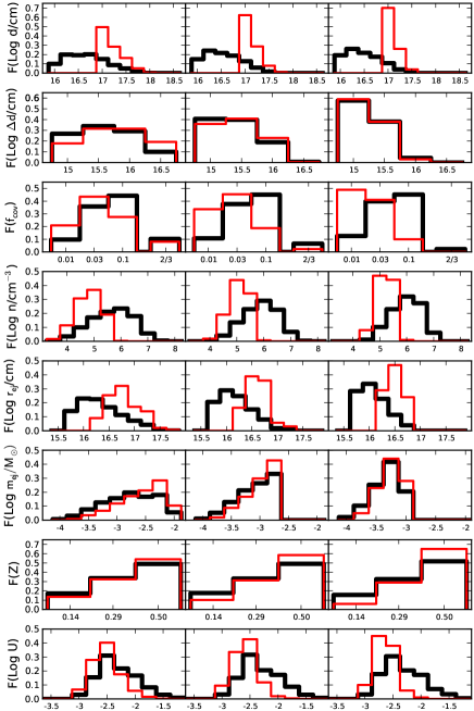
Figure 1: Distribution of parameters for the viable models. Each row shows the distribution of one parameter (see the caption of Table 1; in addition, $U$ is the ionization parameter); columns correspond to different priors on the ejecta mass $m_{\rm ej}$ (left: $\leq 10^{-2}\,{\rm M_{\odot}}$; centre: $\leq 2.5\times 10^{-3}\,{\rm M_{\odot}}$; right: $\leq 10^{-3}\,{\rm M_{\odot}}$). The thick lines refer to all the viable models within the $m_{\rm ej}$ limit, whereas the thin (red on the web) lines further require the distance $d$ of the nova from the XRS to be $\geq 10^{17}\,{\rm cm}$. The distributions are normalized to the number of viable models satisfying the relevant prior (so, the thin line is often above the thick line even if it refers to a lower number of viable models).

4 Comparison of models and data for RZ 2109

Models were required to agree with two basic observational constraints from the spectrum shown in Z08

1. the flux of the [OIII]$\lambda 5007$ line, $F_{5007}\simeq 4.4\times 10^{-16}$. Z08 do not quote an error on this measurement: the equivalent width comparison performed by S11 suggests an uncertainty of 20–30 per cent; but the discrepancy with the Z07 spectrum suggests a larger amount. Furthermore, we account for the approximations of the ionization models by increasing such uncertainty. Thus, we consider viable models with $F_{5007}$ within a factor of 3 from the Z08 estimate.

2. The absence of any other emission lines in all the spectra: we exclude all the models where the luminosity in any optical line exceeds $0.1L_{5007}$.

About 4 per cent of the models we calculated satisfy the above criteria. In Fig. 1, we show the distribution of the various parameters (including the ionization parameter, defined as the number ratio of ionizing photons to H atoms, $U=Q(H)/(4\pi d^{2}cn)$, where $Q(H)$ is the number of ionizing photons - i.e. with energy $\geq 13.6\,{\rm eV}$ - emitted by the XRS in the unit time) for these viable models, and how these distributions are influenced by the choice of priors about the models (e.g. the effects of using different thresholds on the ejecta mass, or imposing a minimum for the nova-XRS distance). Such distributions show us where a large amount of parameter space is available. It can be seen that:

1. it is almost impossible to have viable models if $d\lower 2.15277pt\hbox{$\;\buildrel>\over{\sim}\;$}10^{17.5}\,{\rm cm}\simeq 0.1\,{\rm pc}$;

2. thin shells ($\Delta d\lower 2.15277pt\hbox{$\;\buildrel<\over{\sim}\;$}10^{16}\,{\rm cm}$) are favoured, especially when high-$m_{\rm ej}$ models are excluded;

3. models where the XRS is inside the nova shell (i.e. with $f_{\rm cov}\geq 0.5$) are moderately unlikely, especially when high-$m_{\rm ej}$ models are excluded;

4. shell densities are in the $10^{4}\lower 2.15277pt\hbox{$\;\buildrel<\over{\sim}\;$}n/{\rm cm^{-3}}\lower 2.15277pt\hbox{$\;\buildrel<\over{\sim}\;$}10^{7}$ range; but models with high values of $d$ show a narrower distribution, favouring the low-$n$ part;

5. $Z=0.5$ models are favoured; but it is possible to get reasonable results if $Z=0.29$ or even $Z=0.14$.

6. The ionization parameter is mostly close to $\log(U)\sim-2.5$, a fairly typical value for HII regions; this is somewhat remarkable, as the ionizing spectrum is not produced by hot stars, and most of the radiation energy is in the form of quite energetic (0.1–1 keV) photons (rather than photons just above the Lyman limit).

5 Discussion

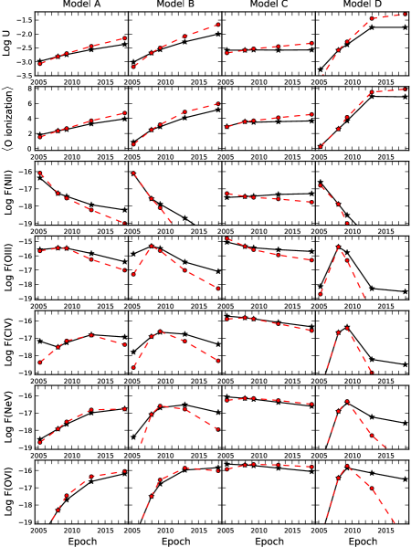
Figure 2: Temporal evolution of model predictions for the four representative models described in the text; solid lines with star symbols are based on assumption (a) (i.e. that the shell thickness is constant), and dashed lines with round symbols (red on the web) are based on assumption (b) (i.e. that shell thickness is proportional to the ejecta radius). Each column refers to one of those models (model A to model D, from left to right), and all the plots have time on the x-axis. On the y-axis we show the ionization parameter $U$ (this is actually an assumption of the model, rather than a prediction; first row from the top), the average ionization stage of oxygen (i.e. $\sum_{i}{(if_{{\rm O,}i})}$, where $f_{{\rm O,}i}$ is the fraction of O atoms that is ionized $i$ times; second row), and the flux at Earth (in ${\rm erg\,s^{-1}\,cm^{-2}}$) of five different lines or groups of lines ([NII]$\lambda 6583$Å, third row; [OIII]$\lambda$5007Å, fourth row; CIV$\lambda\lambda 1549,1551$Å, fifth row; [NeV]$\lambda 3426$Å, sixth row; the complex of OVI lines between $\lambda 1032$Å and $\lambda 1038$Å, seventh row).

Table 2: Parameters of selected models.

Parameter	Model A	Model B	Model C	Model D
$\log{d}$ [cm]	17.25	17.00	16.75	16.50
$\log{\Delta d}$ [cm]	15.5	15.0	15.0	15.5
$f_{\rm cov}$	0.03	0.03	2/3	0.10
$\log{n}$ [cm-3]	4.7	5.5	5.0	5.5
$\log{U(13.6{\rm eV})}$	-2.81	-2.68	-2.58	-2.58
$Z$	0.50	0.29	0.50	0.29
${\log{n_{\rm H}}}$ [cm-2]	21	20	21.5	21.5
$m_{\rm ej}$ [10-4 M⊙]	10.6	6.7	14.9	7.0
$r_{\rm ej}$ [1016 cm]	6.2	3.5	5.6	2.0
$t_{\rm nova}$ [yr]	13.1	7.4	11.9	4.2

Parameters not included in this list (e.g. $L_{0.2-10}$) are fixed at the values in Table 1; the values given here refer to the epoch of the Z08 spectrum (December 2007). The estimate of $t_{\rm nova}$ assumes $v_{\rm ej,3}=1.5$.

5.1 Predictions

[OIII] emission should evolve on a timescale $t_{\rm nova}$. Thus, our scenario can be tested by monitoring the RZ 2109 spectrum.

We arbitrarily select four viable models (see Table 2) for a study of the time evolution of line emission. This was done by assuming that the nova shell keeps expanding with $v_{\rm ej,3}\simeq 1.5$ (cfr. Z08, S11), and properly scaling the relevant parameters ($f_{\rm cov}$, $\Delta d$ and $n$ if XRS is outside the expanding shell; $d$, $\Delta d$ and $n$ otherwise). As the evolution of the thickness $\Delta d$ of the nova shell is unclear, we consider two different cases: (a) $\Delta d=$constant (appropriate for small velocity dispersions within the ejecta), and (b) $\Delta d\propto r_{\rm ej}$ (appropriate for a significant ejecta velocity dispersion).

We calculated the properties of each of these four models at five times: three past epochs (April 2005, December 2007, and March 2009, i.e. the times of the last Z07 observation, of the Z08 observation, and of the last S11 observation, respectively), and two future ones (December 2012 and December 2017, i.e. 5 and 10 years after the Z08 observation). The behaviour of the results are summarized in Fig. 2, where we show the time evolution of the ionization parameter, of the ionization state of Oxygen, and of the intensities of five lines (or groups of lines). Such lines are representative of the main ionization stages and of the most abundant heavy elements in the ejecta, but are not always the most intense: an exhaustive list of possibly detectable optical and UV lines can be found in the Appendix.

In 7 out of 8 models the ionization parameter increases with time, so that heavy elements (such as oxygen) move to higher ionization states. Therefore, high-ionization lines (such as the OVI lines around $\lambda$1035Å) tend to grow stronger, whereas low-ionization lines (e.g. [NII]$\lambda\lambda$6548,6583Å) tend to weaken with time, and intermediate-ionization lines (e.g. the CIV doublet at $\lambda\lambda$1549,1551Å) grow to a peak, and then start to decline.

The case (a) of model C is the main exception: since it assumes that (i) the XRS is within the expanding shell, and (ii) the shell thickness is constant, the density evolution in the shell ($n\propto r_{\rm ej}^{-2}$) compensates the geometrical dilution of the ionizing flux, resulting in a constant ionization parameter. As a consequence, the ionization state of Oxygen (and of all the other heavy elements) remains practically constant, and line fluxes tend to decrease very slowly.

The four models were required to agree with the December 2007 observations, so their spectra for this epoch are dominated by the [OIII] doublet, with $F_{5007}$ within 20 per cent from the Z08 value. In addition, [NeIII]$\lambda 3869$ and [OIII]$\lambda 4363$ might be strong enough to be detectable: the latter was marginally detected by Z08; as to [NeIII], we note that the Z08 spectrum is very noisy at $\lambda\lower 2.15277pt\hbox{$\;\buildrel<\over{\sim}\;$}$4000Å, and this line might be confused with other features in that region. All the models (except model D - see next subsection) are in quite satisfactory agreement with the 2009 observation, too: this is simply because the 1.3 years interval from December 2007 to March 2009 is a relatively small fraction of $t_{\rm nova}$.

Instead we find larger (and more interesting) differences if we look at the April 2005 spectrum: models A and C predict that the [OIII] emission was as strong (A) or stronger (C) than in 2007, and require that the discrepancy among the fluxes reported by Z07 and Z08 derives from observational factors only. Instead, models B and D provide a different explanation: their quite short $t_{\rm nova}$ imply large differences in $r_{\rm ej}$: in 2005 $r_{\rm ej}$ was only 2/3 (model B) or 1/3 (model D) of its value in 2007; such a difference not only reduces the amount of energy intercepted by the ejecta, but at the same time lowers the ionization parameter, favouring low-ionization states and moving the emission from [OIII] to [OII] (or even [OI]) lines.

The predictions for 2012 and 2017 offer an opportunity to test these models, with model D predicting that all anomalous emission lines should disappear before 2012, model B predicting large declines, and models A and C predicting a slower, steady decline. As we already mentioned, such decline is mostly understood in terms of an increasing ionization parameter, so that the O⁺⁺ abundance drops.

5.1.1 Modelling issues

It should be noted that all the above predictions suffer from a number of approximations:

1. The structure of a nova shell is not uniform. There are large density fluctuations both at early times ($\lower 2.15277pt\hbox{$\;\buildrel<\over{\sim}\;$}2$ years after the eruption; see e.g. the images of Nova Cygni 1992 in Chochol et al. 1997) and at late times ($\lower 2.15277pt\hbox{$\;\buildrel>\over{\sim}\;$}10$ years after the eruption; see e.g. the images of T Pyx in Shara et al. 1997).

2. The residual nuclear burning on the WD responsible for the nova eruption might produce a significant amount of UV/X-ray photons for a few years (see Henze et al. 2010): furthermore, when $t_{\rm nova}\lower 2.15277pt\hbox{$\;\buildrel<\over{\sim}\;$}2{\rm yr}$, $r_{\rm ej}\leq 10^{16}{\rm cm}\ll d$, and even moderate WD luminosities (say $L_{\rm X,WD}\sim 10^{38}\,{\rm erg\,s^{-1}\,cm^{-2}}$) are enough for the WD emission to dominate over the one from the XRS. Therefore, the predictions for model B in 2005, for model D in 2007, and especially for model D in 2005 might suffer from the fact that our models do not consider the WD emission.

3. The Cloudy calculations assume steady state, but models with a long ($\;\buildrel>\over{\sim}\;$1 yr) recombination timescale would require a time-dependent approach. For H recombination, $t_{\rm rec,H}\sim(\alpha_{\rm A}n)^{-1}\simeq 0.8\,(n/10^{5}\,{\rm cm^{-3}})^{-1}{\rm yr}$ (where $\alpha_{\rm A}\sim 4\times 10^{-13}\,{\rm cm^{3}\,s^{-1}}$ is the H recombination coefficient), so that models with $n\lower 2.15277pt\hbox{$\;\buildrel<\over{\sim}\;$}10^{5}\,{\rm cm^{-3}}$ might suffer from this problem; however, the recombination timescales of highly ionized metals are shorter (by factors of 2–10) than $t_{\rm rec,H}$, and predictions about their lines should be reliable for $n\lower 2.15277pt\hbox{$\;\buildrel>\over{\sim}\;$}10^{4}\,{\rm cm^{-3}}$.

4. Our geometry is extremely simple, and might suffer from assuming that the whole nova shell is at the same distance from the XRS: this is reasonable if the XRS is within the shell (model C), or if $r_{\rm ej}\ll d$, but there are a number of cases (models A and B at the 2012 and 2017 epochs; model D at all epochs except 2005) where $r_{\rm ej}\geq d/2$ (so that the ionization parameter in the XRS-approaching part of the shell might be $\geq 9$ times higher than in the XRS-receding part).

5. The timing of the evolution depends upon the exact value of $v_{\rm ej,3}$: the adopted 1.5 value is reasonable (S11 estimates $v_{\rm ej,3}\simeq 1.3$ for the broad component of the line profile - see the next subsection), but not unique: a lower(higher) choice of $v_{\rm ej}$ would delay(fasten) the predicted evolution (for example, if $v_{\rm ej}=1$, our predictions for December 2012 and December 2017 would apply to June 2015 and December 2022, respectively). This is particularly relevant for Model D: the [OIII] flux if Fig. 2 and Table A4 evolves too rapidly (the 2007 flux agrees with the observations, but both the 2005 and the 2009 fluxes are too low); however, the model should not be discarded (yet) because these discrepancies can still be reconciled using a value of $v_{\rm ej,3}$ ($\simeq 1$) that is still in agreement with the S11 measurements.

Some of these issues might be resolved by adopting more complicated modelling (e.g. assume a spectrum/temporal evolution for the WD emission, use some density distribution, adopt a more realistic geometry, etc.); however, a more detailed modelling, while providing more reliable predictions, would also require us to introduce a number of additional parameters. This is not only a problem in terms of resources (such as computing power), but would further complicate the interpretation of the results.

5.2 Line profile

S11 model the spectral profile of the [OIII]$\lambda\lambda 4959,5007$ complex as the superposition of the identical profiles of the two lines of the doublet, each one made of a central, relatively narrow (FWHM$\sim 300\,{\rm km\,s^{-1}}$) gaussian peak, plus a much broader (FWHM$\sim 1300\,{\rm km\,s^{-1}}$) ‘flat’ component (possibly the result of a bipolar outflow); notably, the latter component is not really flat: the red side is about 1.4 times brighter than the blue side. As noted by S11, this is consistent with a nova shell between the XRS and the observer. If this is the case, the flux difference among the two sides suggests that in 2007-2008 $r_{\rm ej}$ was of the order of 10 per cent of the distance between the nova and the XRS: this would favor models with $f_{\rm cov}\sim$ 0.01. Furthermore, since $r_{\rm ej}$ increases with time, the asymmetry between the red and blue sides should increase as well (at least as long as the XRS is outside the nova shell).

If the nova lies between us and the XRS, the ejecta might even intercept the line of sight to the XRS, increasing the value of $N_{\rm H}$. We checked whether such an increase can explain the fading of the XRS seen in the 2004 XMM observation (see M2007), and in the subsequent Swift and Chandra observations (see Maccarone et al. 2010). The effective X-ray extinction due to isotropic nova ejecta is

$$N_{\rm H,shell} =g{m_{\rm ej}\over{4\pi r_{\rm ej}^{2}m_{\rm H}}}{Z\over Z_{\odot}}\simeq$$ (1)

$$\simeq 4.2\times 10^{22}{\rm cm^{-2}}\left({g\over 3}\right)\left({m_{\rm ej}\over{10^{-3}\,{\rm M_{\odot}}}}\right)\left({r_{\rm ej}\over{10^{16}\,{\rm cm}}}\right)^{-2}\left({Z\over{0.29}}\right)$$

where $g$ is a geometrical factor accounting for the number of times that the photons cross the shell (1 if the XRS is within the shell; 2 if the XRS is outside the shell), and for the inclination of the photon direction with respect to the normal to the shell (note that $g$ can be quite larger than 2 if the line of sight to the XRS is almost tangential to the ejecta shell). Maccarone et al (2010) suggest that the weakness of the XRS in RZ 2109 during the Chandra 2010 observation might be explained by a large increase in the effective $N_{\rm H}$ in front of the XRS. We used the web version of W3PIMMS (http://heasarc.nasa.gov/Tools/w3pimms.html) to estimate that $N_{\rm H}\lower 2.15277pt\hbox{$\;\buildrel>\over{\sim}\;$}3\times 10^{22}\,{\rm cm^{-2}}$ is necessary to explain the Chandra 2010 observations. This is marginally consistent with our scenario: if we set $g=6$, $Z=0.50$, $m_{\rm ej}=2.2\times 10^{-3}\,{\rm M_{\odot}}$, we can obtain such a high $N_{\rm H}$ for $r_{\rm ej}\lower 2.15277pt\hbox{$\;\buildrel<\over{\sim}\;$}3\times 10^{16}\,{\rm cm}$. In turn, this implies that the nova eruption occurred in 2000–2004 (for $1\lower 2.15277pt\hbox{$\;\buildrel<\over{\sim}\;$}v_{\rm ej,3}\lower 2.15277pt\hbox{$\;\buildrel<\over{\sim}\;$}1.5$ ), which might be consistent with the timing of the Z07 observations (2004–2005). However, the available parameter space is very small: a slight change in the choice of $g$, $Z$ and $m_{\rm ej}$ can reduce the upper limit on $r_{ej}$, moving the nova occurrence to an epoch after the first Z07 observation. Therefore, we deem quite unlikely that the weakening of the XRS is (entirely) due to the additional absorption from the nova shell; however, if this is the case, the XRS should re-brighten within a few years.

5.3 Probability

We estimate the probability of having a nova shell with properties suitable to explain the RZ 2109 observations within a distance $\tilde{d}$ from the XRS as

$$p(<\tilde{d}) =\Gamma_{E}\gamma_{\rm GC}(N_{\rm GC}\langle m_{\rm GC}\rangle)\,\left({{{4\pi}\over 3}\tilde{d}^{3}}\right){{n_{\rm*,c}}\over{N_{\rm GC}}}\,\tilde{f}\,t_{\rm nova}\sim$$ (2)

$$\sim 5\times 10^{-9}\,\gamma_{\rm GC}\,{{\langle m_{\rm GC}\rangle}\over{0.5{\rm M_{\odot}}}}\,\left({{\tilde{d}}\over{0.1{\rm pc}}}\right)^{3}\,{{n_{\rm*,c}}\over{10^{5}{\rm pc^{-3}}}}\,{{\tilde{f}}\over{0.01}}\,{{r_{\rm ej}}\over{0.01{\rm pc}}}\,v_{\rm ej,3}^{-1},$$

where $\Gamma_{E}$ and $\gamma_{\rm GC}$ were introduced in Sec. 2, $N_{\rm GC}$ is the number of stars in a GC, $\langle m_{\rm GC}\rangle$ is the average stellar mass in a GC, $n_{\rm*,c}$ is the number density of stars at the centre of a GC ($10^{4}$–$10^{6}\,{\rm pc^{-3}}$; see e.g. Pryor & Meylan 1993), $\tilde{f}$ is the fraction of novae whose ejecta can produce the observed line emission (a highly uncertain quantity; since relatively massive ejecta are needed, we use 0.01 as a reference), and $t_{\rm nova}\sim 10\,{\rm yr}[r_{\rm ej}/(0.01\,{\rm pc})]v_{\rm ej,3}^{-1}$ acts as the visibility timescale for the [OIII] line emission.

Such a probability is of the same order of magnitude as that predicted in other scenarios such as the disruption of a WD by an IMBH (Clausen & Eracleous 2011 quote a disruption rate of $\sim 10^{-8}\,{\rm yr^{-1}\,GC^{-1}}$ from Sigurdsson & Rees 1997), and it must be noted that the large uncertainty about several parameters in the above formula might lead to a substantial increase of $p(<\tilde{d})$.

We note that, if the XRS is outside the nova shell, a further factor $\Omega/4\pi$ accounting for the possible beaming of the XRS radiation should be introduced into eq. (2): therefore, an observational confirmation of this scenario might disfavour the models of the XRS (e.g. King 2011) that assume a beamed emission.

6 Summary and conclusions

We used the photoionization code Cloudy to check whether the peculiar emission spectra from XRS-hosting GCs (especially RZ 2109) can be explained as the result of the photoionization of a nova shell by the radiation emitted by the XRS. We found that this is definitely possible, but requires that the nova ejecta are relatively massive ($\lower 2.15277pt\hbox{$\;\buildrel>\over{\sim}\;$}0.5\times 10^{-3}\,{\rm M_{\odot}}$), and that the XRS-nova distance is quite small ($\lower 2.15277pt\hbox{$\;\buildrel<\over{\sim}\;$}0.1\,{\rm pc}$).

The combination of these two requirements is quite unlikely; on the other hand, it can explain observations in a straightforward manner (although the line profile needs further investigation). While not entirely satisfactory, this compares well with the two other proposed scenarios for RZ 2109: (i) the disruption of a WD by an IMBH (an event as unlikely as the one we discuss) explains the line profile and the absence of H lines (I10, Clausen & Eracleous 2011), but appears to be unable to produce the high [OIII] luminosity (Porter 2010, S11); (ii) the ionization of material ejected from the XRS itself, while not suffering from the “unlikely coincidence” problem, does not explain either the absence of H emission lines, nor some properties of the line profile (asymmetry in the flat component, origin of the gaussian component).

Finally, we predict the future evolution of the line emission in the XRS+nova scenario, by looking at both optical and UV lines. We find that in most cases the nova shell tends to move towards a higher ionization state, so that the line flux should move from moderate-ionization lines such as [OIII]$\lambda 5007$Å to high-ionization lines (e.g. the OVI lines in the 1032–1038Å wavelength range). Such predictions might provide a crucial test for discriminating among the various hypotheses described above.

Appendix A Full predictions - Tables

In this appendix, we list the detailed predictions about line fluxes at Earth, and about the properties of the nova ejecta (e.g. the ionization state of C, N, O, and Ne) from the four models described in the text, evolved to five past or future epochs: April 2005, December 2007, March 2009 (chosen to coincide with the times of past optical observations), December 2012, and December 2017.

We report all the emission lines in the UV-optical range (913Å$\leq\lambda\leq$10000Å) reaching a flux $\geq 5\times 10^{-18}\,{\rm erg\,s^{-1}\,cm^{-2}}$ in at least one of the five considered epoch, plus Lyman$\alpha$ and H$\alpha$. For well-separated multiplets we list only the strongest line (for example, in the case of the [OIII]$\lambda\lambda$4959,5007Å doublet we only list [OIII]$\lambda$5007Å), whereas close multiplets are listed as a single line (for example the [OII]$\lambda\lambda$3726,3729Å doublet is listed as [OII]$\lambda$3727Å). All the fluxes are in units of $10^{-16}\,{\rm erg\,s^{-1}\,cm^{-2}}$, and were obtained assuming a distance $D=16\,{\rm Mpc}$. No reddening correction was applied.

All the data columns - except the one referring to the Z08 observation, which is taken as a reference point - report two set of data: the first was obtained assuming that the shell thickness $\Delta d$ remains constant at the value used for December 2007 (implying that the density $n$ scales as $r_{\rm ej}^{-2}$;assumption a), whereas the second was obtained assuming that $\Delta d$ increases linearly with time (i.e. that $\Delta d/r_{\rm ej}$ remains constant at the value estimated for December 2007; in such case the density $n$ scales as $r_{\rm ej}^{-3}$; assumption b). The two cases are generally separated by a “/”, but in the case of ionization states it was necessary to use two separate lines.

Table 3: Evolution of emission line fluxes and other physical properties for model A.

Line	April 2005	December 2007	March 2009	December 2012	December 2017
Model A - Spectral lines
NIII$\lambda 991$	0.020/0.014	0.043	0.063/0.074	0.129/0.094	0.077/0.026
OVI$\lambda 1032$–$1038$	0/0	0.005	0.020/0.035	0.232/0.446	0.654/0.900
Lyman $\alpha$ $\lambda 1216$	0.168/0.182	0.103	0.081/0.072	0.045/0.033	0.029/0.018
OV]$\lambda 1218$	0/0	0.004	0.011/0.016	0.076/0.131	0.170/0.178
NV$\lambda 1239,1243$	0.005/0.002	0.055	0.131/0.189	0.667/0.878	0.977/0.704
OIV]$\lambda 1402$	0.004/0.002	0.038	0.090/0.130	0.460/0.548	0.516/0.279
NIV]$\lambda 1486$	0.012/0.006	0.081	0.172/0.235	0.714/0.770	0.647/0.267
CIV$\lambda 1549,1551$	0.068/0.004	0.031	0.057/0.071	0.162/0.151	0.119/0.043
OIII]$\lambda 1661,1666$	0.030/0.020	0.092	0.135/0.147	0.168/0.088	0.073/0.025
NIII$\lambda 1750$	0.067/0.046	0.196	0.286/0.314	0.383/0.203	0.146/0.037
CIII]$\lambda 1907,1909$	0.026/0.022	0.059	0.078/0.082	0.092/0.049	0.033/0.007
$[$NeIV]$\lambda 2424$	0.007/0.003	0.041	0.085/0.114	0.326/0.348	0.310/0.156
$[$OII]$\lambda 2471$	0.050/0.100	0.014	0.011/0.008	0.004/0.002	0.002/0.001
$[$NeV]$\lambda 3426$	0.003/0.002	0.012	0.023/0.031	0.103/0.153	0.178/0.171
$[$OII]$\lambda 3727$	0.055/0.098	0.012	0.010/0.008	0.005/0.002	0.003/0.001
$[$NeIII]$\lambda 3869$	0.166/0.148	0.232	0.242/0.229	0.139/0.058	0.041/0.010
$[$OIII]$\lambda 4363$	0.030/0.023	0.058	0.071/0.071	0.056/0.025	0.019/0.006
$[$OIII]$\lambda 5007$	2.77/2.24	3.6	3.43/3.14	1.48/0.555	0.385/0.097
$[$NII]$\lambda 5755$	0.023/0.053	0.005	0.004/0.003	0.001/0.001	0.001/0
H$\alpha$ $\lambda 6563$	0.014/0.015	0.008	0.006/0.004	0.003/0.002	0.002/0.001
$[$NII]$\lambda 6583$	0.433/0.893	0.055	0.037/0.029	0.012/0.006	0.006/0.001
$[$OII]$\lambda 7325$	0.068/0.140	0.019	0.015/0.012	0.006/0.003	0.003/0.001
Model A - Model parameters and ionization conditions
$\log{n}$ [cm-3]	4.87/4.96	4.70	4.63/4.59	4.45/4.33	4.26/4.04
$t_{\rm nova}\,{\rm[yr]}$	10.4	13.1	14.4	18.1	23.1
$r_{\rm ej}\,{\rm[10^{16}cm]}$	4.9	6.2	6.8	8.6	10.9
$f_{\rm cov}$	0.020	0.030	0.0354	0.533	0.0831
$\log{U(13.6{\rm eV})}$	-2.98/-3.07	-2.81	-2.74/-2.70	-2.56/-2.44	-2.37/-2.15
C(I$\rightarrow$VII)	-,11,69,6,13,1,-	-,3,55,11,27,4,0	-,2,45,13,33,7,0	-,0,17,12,45,23,2	-,0,5,6,40,40,9
	0,31,56,5,8,0,-		-,1,40,13,36,9,1	-,0,8,9,44,33,5	-,0,1,2,26,50,21
N(I$\rightarrow$VIII)	0,25,63,7,4,1,-,-	-,2,70,15,9,4,0,-	-,1,61,20,11,7,1,-	-,0,24,30,15,25,5,0	-,0,7,21,14,40,16,1
	3,48,42,4,2,0,-,-		-,1,56,22,12,9,1,-	-,0,11,28,15,35,10,1	-,0,2,9,9,43,32,5
O(I$\rightarrow$IX)	0,31,58,9,2,0,0,-,-	-,2,69,23,4,2,0,-,-	-,1,58,31,6,3,1,-,-	-,0,19,53,13,10,5,0,-	-,0,6,41,20,15,15,2,0
	3,52,39,6,1,0,-,-,-		-,1,53,35,7,4,1,0,-	-,0,8,50,18,13,10,1,-	-,-,2,22,20,17,30,8,0
Ne(I$\rightarrow$XI)	0,25,69,5,1,0,-,-,-,-,-	-,1,79,15,3,0,-,-,-,-,-	-,1,70,23,5,1,-,-,-,-,-	-,0,29,49,19,3,0,-,-,-,-	-,0,10,44,36,9,1,0,0,-,-
	2,39,55,3,1,-,-,-,-,-,-		-,1,65,27,7,1,0,-,-,-,-	-,0,13,50,30,6,1,0,-,-,-	-,-,3,26,47,18,4,1,1,0,-

Fluxes are in units of $10^{-16}\,{\rm erg\,s^{-1}\,cm^{-2}}$ and assume D=16 Mpc (no reddening). Wavelengths are in Å, and in case of multiplets only the strongest component(s) are listed. The ionization states of C,N,O, and Ne are described by listing the percentages of each ionic state with respect to the total (with “0” indicating a percentage between 0.05% and 0.5%, and “-” indicating a percentage below 0.05%). See text for more details

Table 4: Evolution of emission-line fluxes and other physical properties for model B.

Line	April 2005	December 2007	March 2009	December 2012	December 2017
Model B - Spectral lines
NIII$\lambda 991$	0.010/0.002	0.132	0.216/0.220	0.115/0.042	0.038/0.005
OVI$\lambda 1032$–$1038$	0/0	0.032	0.167/0.285	1.06/1.39	1.47/0.961
Lyman $\alpha$ $\lambda 1216$	0.523/0.872	0.342	0.245/0.208	0.136/0.094	0.095/0.057
OV]$\lambda 1218$	0/0	0.034	0.118/0.173	0.371/0.287	0.234/0.073
NV$\lambda 1239,1243$	0.009/0.002	0.252	0.744/1.01	1.76/1.30	1.09/0.301
OIV]$\lambda 1402$	0.007/0.001	0.181	0.495/0.637	0.607/0.268	0.200/0.030
NIV]$\lambda 1486$	0.020/0.002	0.341	0.850/1.07	0.982/0.420	0.303/0.040
CIV$\lambda 1549,1551$	0.016/0.002	0.127	0.228/0.250	0.175/0.068	0.045/0.005
OIII]$\lambda 1661,1666$	0.067/0.003	0.306	0.347/0.285	0.077/0.024	0.022/0.002
NIII$\lambda 1750$	0.140/0.006	0.655	0.809/0.710	0.221/0.065	0.056/0.004
CIII]$\lambda 1907,1909$	0.074/0.053	0.144	0.151/0.128	0.035/0.009	0.006/0
NII]$\lambda 2141$	0.205/0.316	0.014	0.009/0.006	0.003/0.001	0/0
CII]$\lambda 2324-2329$	0.067/0.114	0.007	0.004/0.003	0.001/0	0/0
$[$NeIV]$\lambda 2424$	0.005/0	0.087	0.180/0.206	0.132/0.046	0.028/0.002
$[$OII]$\lambda 2471$	0.546/0.798	0.024	0.011/0.006	0.002/0	0/0
$[$NeV]$\lambda 3426$	0.004/0	0.083	0.204/0.256	0.303/0.168	0.110/0.011
$[$OII]$\lambda 3727$	0.070/0.076	0.004	0.002/0.001	0.001/0	0/0
$[$NeIII]$\lambda 3869$	0.316/0.305	0.358	0.231/0.156	0.017/0.003	0.002/0
$[$OIII]$\lambda 4363$	0.071/0.003	0.206	0.176/0.129	0.024/0.006	0.005/0
$[$OIII]$\lambda 5007$	1.37/0.050	4.84	3.36/2.33	0.368/0.095	0.080/0.005
$[$NII]$\lambda 5755$	0.333/0.500	0.013	0.006/0.004	0.001/0	0/0
$[$OI]$\lambda 6300$	0.336/0.581	0	0/0	0/0	0/0
H$\alpha$ $\lambda 6563$	0.027/0.030	0.025	0.017/0.014	0.008/0.005	0.004/0.002
$[$NII]$\lambda 6583$	0.748/0.812	0.027	0.013/0.008	0.004/0.001	0.001/0
$[$OII]$\lambda 7325$	0.726/1.06	0.033	0.015/0.009	0.002/0	0/0
Model B - Model parameters and ionization conditions
$\log{n}$ [cm-3]	5.83/6.00	5.50	5.38/5.32	5.10/4.90	4.82/4.48
$t_{\rm nova}\,{\rm[yr]}$	4.7	7.4	8.7	12.4	17.4
$r_{\rm ej}\,{\rm[10^{16}cm]}$	2.2	3.5	4.1	5.9	8.2
$f_{\rm cov}$	0.0139	0.030	0.0399	0.0759	0.1429
$\log{U(13.6{\rm eV})}$	-3.01/-3.18	-2.68	-2.56/-2.50	-2.28/-2.08	-2.00/-1.66
C(I$\rightarrow$VII)	1,60,33,2,3,0,-	-,2,41,14,36,6,0	0,1,24,14,47,14,1	-,0,4,7,44,39,6	-,0,1,2,26,52,19
	2,74,24,0,0,-,-		-,0,18,13,49,19,1	-,0,1,3,32,50,14	-,-,0,0,9,46,46
N(I$\rightarrow$VIII)	20,63,14,2,1,0,-,-	-,1,65,19,9,5,0,-	-,1,43,29,14,13,1,-	-,0,7,23,18,40,11,1	-,0,2,8,11,46,29,3
	33,66,1,0,-,-,-,-		-,0,32,31,15,18,2,0	-,0,3,11,14,48,23,2	-,-,0,1,3,30,50,15
O(I$\rightarrow$IX)	32,52,13,2,0,-,-,-,-	-,1,62,28,6,2,1,-,-	-,0,36,44,11,6,2,0,-	-,0,4,34,25,18,17,1,-	-,-,1,12,18,22,40,8,0
	43,56,0,-,-,-,-,-,-		-,0,25,49,14,8,4,0,-	-,-,1,16,22,23,33,5,0	-,-,0,2,6,11,52,26,2
Ne(I$\rightarrow$XI)	5,39,52,3,0,-,-,-,-,-,-	-,1,60,28,10,2,0,-,-,-,-	-,0,33,38,23,6,1,0,-,-,-	-,-,3,20,42,27,6,2,1,0,-	-,-,0,5,24,36,19,10,6,0,-
	8,47,45,0,-,-,-,-,-,-,-		-,0,22,39,29,9,1,0,-,-,-	-,-,1,8,32,36,14,6,3,0,-	-,-,-,0,4,15,20,24,35,1,0

See the caption of Table A1 for the definition of symbols and units.

Table 5: Evolution of emission-line fluxes and other physical properties for model C.

Line	April 2005	December 2007	March 2009	December 2012	December 2017
Model C - Spectral lines
CIII$\lambda 977$	0.349/0.308	0.284	0.247/0.223	0.175/0.125	0.116/0.069
NIII$\lambda 991$	1.140/1.130	0.878	0.751/0.656	0.529/0.348	0.359/0.180
OVI$\lambda 1032$–$1038$	2.360/1.180	2.090	1.920/2.270	1.380/2.090	0.880/1.620
Lyman $\alpha$ $\lambda 1216$	0.332/0.448	0.212	0.178/0.161	0.121/0.088	0.078/0.044
OV]$\lambda 1218$	0.890/0.505	0.717	0.631/0.722	0.413/0.550	0.240/0.331
NV$\lambda 1239,1243$	4.930/3.100	4.240	3.810/4.160	2.670/3.070	1.690/1.790
OIV]$\lambda 1402$	3.850/2.590	3.160	2.730/2.740	1.760/1.570	1.030/0.736
NIV]$\lambda 1486$	6.590/4.400	5.400	4.640/4.640	2.960/2.510	1.690/1.060
CIV$\lambda 1549,1551$	1.940/1.300	1.570	1.340/1.340	0.842/0.694	0.467/0.282
OIII]$\lambda 1661,1666$	1.150/1.580	0.733	0.605/0.473	0.439/0.230	0.321/0.115
NIII$\lambda 1750$	3.210/4.040	2.200	1.820/1.450	1.280/0.659	0.889/0.295
CIII]$\lambda 1907,1909$	1.230/1.470	0.867	0.722/0.581	0.497/0.261	0.329/0.114
$[$OIII]$\lambda 2321$	0.113/0.184	0.059	0.047/0.034	0.032/0.015	0.022/0.006
$[$NeIV]$\lambda 2424$	1.520/1.000	1.460	1.340/1.340	0.982/0.855	0.637/0.447
$[$NeV]$\lambda 3426$	0.865/0.546	0.713	0.631/0.705	0.423/0.536	0.248/0.322
$[$NeIII]$\lambda 3869$	0.964/1.620	0.528	0.425/0.315	0.301/0.130	0.218/0.055
$[$OIII]$\lambda 4363$	0.485/0.789	0.254	0.200/0.149	0.136/0.063	0.095/0.028
$[$OIII]$\lambda 5007$	9.350/16.90	4.630	3.720/2.680	2.730/1.150	2.050/0.498
H$\alpha$ $\lambda 6563$	0.023/0.033	0.014	0.012/0.010	0.008/0.006	0.005/0.003
$[$NII]$\lambda 6583$	0.032/0.054	0.036	0.038/0.032	0.048/0.026	0.056/0.017
Model C - Model parameters and ionization conditions
$\log{n}$ [cm-3]	5.19/5.29	5.00	4.92/4.88	4.73/4.60	4.52/4.28
$t_{\rm nova}\,{\rm[yr]}$	9.2	11.9	13.2	16.9	21.9
$r_{\rm ej}\,{\rm[10^{16}cm]}$	4.3	5.6	6.2	8.0	10.3
$f_{\rm cov}$	2/3	2/3	2/3	2/3	2/3
$\log{U(13.6{\rm eV})}$	-2.58/-2.68	-2.58	-2.57/-2.53	-2.58/-2.45	-2.57/-2.33
C(I$\rightarrow$VII)	-,1,34,17,37,11,1	-,1,26,17,41,14,1	-,1,24,17,42,15,2	-,2,25,15,42,15,2	-,2,26,14,41,15,2
	-,1,50,14,28,6,0		-,1,20,16,44,18,2	-,1,13,12,45,25,4	-,1,10,8,41,33,8
N(I$\rightarrow$VIII)	-,0,30,34,12,20,4,0	-,0,21,35,13,25,5,0	-,0,20,34,14,26,6,0	-,1,20,32,14,27,6,1	-,1,23,29,14,26,7,1
	-,0,49,27,10,12,2,0		-,0,15,33,14,29,8,1	-,0,10,26,14,36,13,1	-,0,8,17,12,39,21,3
O(I$\rightarrow$IX)	-,0,21,51,12,9,6,1,-	-,0,12,53,15,12,8,1,-	-,0,11,51,15,12,8,1,-	-,0,12,48,16,13,9,1,-	-,1,14,45,16,13,10,2,0
	-,0,39,42,9,6,3,0,-		-,0,8,49,17,13,10,2,0	-,0,6,39,19,15,17,4,0	-,0,5,28,18,16,24,8,1
Ne(I$\rightarrow$XI)	-,0,29,48,19,4,1,0,-,-,-	-,0,20,52,23,5,1,0,-,-,-	-,0,18,52,24,5,1,0,0,-,-	-,0,20,49,24,5,1,0,0,-,-	0,0,23,47,23,5,1,0,0,-,-
	-,0,49,37,12,2,0,0,-,-,-		-,0,14,51,28,6,1,0,0,-,-	0,0,10,44,35,9,2,1,0,-,-	-,0,8,36,40,12,3,1,1,0,-

See the caption of Table A1 for the definition of symbols and units.

Table 6: Evolution of emission-line fluxes and other physical properties for model D.

Line	April 2005	December 2007	March 2009	December 2012(a)	December 2017(a)
Model D - Spectral lines
CIII$\lambda 977$	0/0	0.061	0.063/0.039	0.003/0	0.002/0
NIII$\lambda 991$	0/0	0.213	0.208/0.138	0.009/0	0.005/0
OVI$\lambda 1032$–$1038$	0/0	0.371	1.41/1.83	0.714/0.093	0.309/0
Lyman $\alpha$ $\lambda 1216$	0.391/0.411	0.403	0.191/0.145	0.040/0.015	0.023/0
OV]$\lambda 1218$	0/0	0.149	0.492/0.599	0.050/0.003	0.021/0
NV$\lambda 1239,1243$	0/0	0.746	2.01/2.27	0.155/0.013	0.050/0
OIV]$\lambda 1402$	0/0	0.493	1.11/1.09	0.028/0.001	0.014/0
NIV]$\lambda 1486$	0/0	0.784	1.72/1.65	0.018/0.001	0.009/0
CIV$\lambda 1549,1551$	0/0	0.216	0.456/0.391	0.006/0.001	0.003/0
$[$NeIV]$\lambda 1602$	0/0	0.086	0.161/0.142	0.006/0.001	0.003/0
OIII]$\lambda 1661,1666$	0/0	0.296	0.198/0.088	0.003/0	0.002/0
NIII$\lambda 1750$	0.001/0	0.697	0.496/0.251	0.004/0	0.003/0
CIII]$\lambda 1907,1909$	0.008/0.004	0.242	0.173/0.086	0.001/0	0.001/0
NII]$\lambda 2141$	0.118/0.092	0.005	0.002/0.001	0/0	0/0
CII]$\lambda 2324-2329$	0.062/0.063	0.005	0.002/0.001	0/0	0/0
$[$NeIV]$\lambda 2424$	0/0	0.137	0.341/0.348	0.023/0.003	0.013/0
$[$OII]$\lambda 2471$	0.283/0.200	0.007	0.002/0.001	0/0	0/0
MgII$\lambda 2796,2803$	0.065/0.031	0.004	0.001/0	0/0	0/0
$[$NeV]$\lambda 3426$	0/0	0.127	0.394/0.473	0.059/0.005	0.026/0
$[$NeI]$\lambda 3467$	0.056/0.084	0	0/0	0/0	0/0
$[$NeIII]$\lambda 3869$	0.079/0.062	0.355	0.151/0.051	0.001/0	0.001/0
$[$OIII]$\lambda 4363$	0/0	0.173	0.088/0.031	0.001/0	0/0
$[$OIII]$\lambda 5007$	0.007/0.002	4.30	1.73/0.480	0.005/0	0.003/0
$[$NII]$\lambda 5755$	0.185/0.168	0.005	0.001/0.001	0/0	0/0
$[$OI]$\lambda 6300$	0.348/.454	0	0/0	0/0	0/0
H$\alpha$ $\lambda 6563$	0.022/0.030	0.031	0.014/0.010	0.002/0.001	0.001/0
$[$NII]$\lambda 6583$	0.244/0.159	0.013	0.003/0.001	0/0	0/0
$[$OII]$\lambda 7325$	0.375/0.264	0.010	0.003/0.001	0/0	0/0
Model D - Model parameters and ionization conditions
$\log{n}$ [cm-3]	6.20/6.55	5.50	5.30/5.20	4.46/4.15	4.11/3.63
$t_{\rm nova}\,{\rm[yr]}$	1.5	4.2	5.5	9.2	14.2
$r_{\rm ej}\,{\rm[10^{16}cm]}$	0.7	2.0	2.6	4.3(a)	6.7(a)
$f_{\rm cov}$	0.02	0.10	0.160	2/3(a)	2/3(a)
$\log{U(13.6{\rm eV})}$	-3.28/-3.63	-2.58	-2.38/-2.28	-1.76/-1.44	-1.76/-1.28
C(I$\rightarrow$VII)	41,57,2,-,-,-,-	-,2,65,8,20,5,0	-,0,20,12,40,22,4	-,-,0,0,4,30,66	-,-,0,0,5,31,63
	59,40,1,-,-,-,-		-,0,7,10,42,33,8	-,-,-,-,1,15,85	-,-,-,-,-,3,97
N(I$\rightarrow$VIII)	74,26,0,-,-,-,-,-	-,1,68,15,7,8,2,0	-,0,21,27,12,28,10,1	-,-,0,0,0,9,42,48	-,-,0,0,0,9,41,48
	80,20,-,-,-,-,-,-		-,-,7,25,12,36,17,2	-,-,-,-,-,2,23,75	-,-,-,-,-,0,5,95
O(I$\rightarrow$IX)	70,30,0,-,-,-,-,-,-	-,1,64,23,6,4,3,0,-	-,0,18,40,16,11,12,3,0	-,-,0,1,1,2,21,49,26	-,-,0,1,1,2,20,49,26
	76,24,-,-,-,-,-,-,-		-,-,4,39,19,13,18,6,0	-,-,-,-,0,0,6,38,56	-,-,-,-,-,-,0,10,90
Ne(I$\rightarrow$XI)	61,30,10,-,-,-,-,-,-,-,-	-,1,67,21,10,2,0,0,-,-,-	-,0,20,40,31,8,1,1,0,-,-	-,-,0,3,15,21,14,11,27,9,1	-,-,1,3,15,20,13,11,28,9,1
	71,23,6,-,-,-,-,-,-,-,-		-,-,6,38,40,12,3,1,1,0,-	-,-,0,0,2,5,5,6,39,35,6	-,-,-,-,-,-,-,0,8,46,46

See the caption of Table A1 for the definition of symbols and units.
Note: ^(a): In this model, the 2012 and 2017 epochs have $r_{\rm ej}>d$ (the distance between the XRS and the nova), i.e. the XRS becomes engulfed in the expanding nova shell. Then, for these epochs we assume $f_{\rm cov}=2/3$, and use $r_{\rm ej}$ as the distance from the XRS to the shell; this is quite inaccurate, but the emission lines remain very weak also for more detailed calculations.

References

- [1] Allende Prieto C., Lambert D.L., Asplund M., 2001, ApJ, 556, L63
- [2] Allende Prieto C., Lambert D.L., Asplund M., 2002, ApJ, 573, L137
- [3] Brassington N.J., et al., 2010, ApJ, 725, 1805
- [4] Chochol D., Grygar J., Pribulla T., Komzik R., Hric L., Elkin V., 1997, A&A , 318, 908
- [5] Clausen D., Eracleous M., 2011, ApJ, 726, 34
- [6] Della Valle M., Rosino L., Bianchini A., Livio M., 1994, A&A, 287, 403
- [7] Gehrz R.D., Truran J.W., Williams R.E., Starrfield S., 1998, PASP, 110, 3
- [8] Ferland G.J., Shields G.A., 1978, ApJ, 226, 172
- [9] Ferland G.J., Korista K.T., Verner D.A., Ferguson J.W., Kingdon J.B., Verner E.M., 1998, PASP, 110, 761
- [10] Grevesse N., Sauval A.J., 1998, Space Science Review, 85, 161
- [11] Heinke C.O., 2011, to appear in the proceedings of the conference “Binary Star Evolution: Mass Loss, Accretion and Mergers” (eds. V. Kalogera and M. van der Sluys, AIP Conf. Ser.), Mykonos, Greece, June 22-25, 2010, (arxiv.org/1101.5356)
- [12] Holweger H., 2001, Joint SOHO/ACE workshop “Solar and Galactic Composition” (Bern, Switzerland, March 6–9 2001), edited by R.F. Wimmer-Schweingruber, AIPC proceedings, vol. 598, p. 23
- [13] Henze M., et al., 2009, A&A, 500, 769
- [14] Henze M., et al., 2010, A&A, 523, 89
- [15] Iijima T., Naito H., 2011, A&A, 526, A73
- [16] Irwin J.A., Brink T.G., Bregman J.N., Roberts T.P., 2010, ApJ, 712, L1 [I10]
- [17] Kalogera V., Henninger M., Ivanova N., King A.R., 2004, ApJ, 603, L41
- [18] King A., 2011, ApJ, 732, L28
- [19] Maccarone T.J., Kundu A., Zepf S.E., Rhode K.L., 2007, Nature, 445, 183 [M07]
- [20] Maccarone T.J., Kundu A., Zepf S.E., Rhode K.L., 2010, MNRAS, 409, L84
- [21] Maccarone T.J., Kundu A., Zepf S.E., Rhode K.L., 2011, MNRAS, 410, 1655
- [22] Maccarone T.J., Warner B., 2011, MNRAS, 410, L32
- [23] Mannucci F., Della Valle M., Panagia N., Cappellaro E., Cresci G., Maiolino R., Petrosian A., Turatto M., 2005, A&A, 433, 807
- [24] Moore K., Bildsten L., 2011, ApJ, 728, 81
- [25] Peacock M.B., Maccarone T.J., Knigge C., Kundu A., Waters C.Z., Zepf S.E., Zurek D.R., MNRAS, 402, 803
- [26] Pietsch W., et al., 2007, A&A, 465, 375
- [27] Porter R.L., 2010, MNRAS, 407, L59
- [28] Prialnik D., 1986, ApJ, 310, 222
- [29] Pryor C., Meylan G., 1993, in ASP Con ference Series 50, Structure and Dynamics of Globular Clusters, eds Djorgovski S.G. & Meylan G. (San Francisco, CA: ASP), 357
- [30] Shafter A.W, Quimby R.M., 2007, ApJ, 671, L121
- [31] Shara M.M., Zurek D.R., Williams R.E., Prialnik D., Gilmozzi R., Moffat A.F.J., 1997, AJ, 114, 258
- [32] Shara M.M., Zurek D.R., Baltz E.A., Lauer T.R., Silk J., 2004, ApJ, 605, L117
- [33] Shara M.M., Yaron O., Prialnik D., Kovetz A., Zurek D., 2010, ApJ, 725, 831 [S10]
- [34] Shih I.C., Kundu A., Maccarone T.J., Zepf S.E., Joseph T.D., 2010, ApJ, 721, 323
- [35] Sigurdsson S., Phinney E.S., 1995, ApJS, 99, 609
- [36] Sigurdsson S., Rees M.J., 1997, MNRAS, 284, 318
- [37] Starrfield S., Truran J.W., Sparks W.M., Kutter G.S., 1972, ApJ, 176, 169
- [38] Steele M.M., Zepf S.E., Kundu A., Maccarone T.J., Rhode K.L., Salzer J.J., 2011, ApJ, in press (arXiv:1107.4051) [S11]
- [39] Yaron O., Prialnik D., Shara M.M., Kovetz A., 2005, ApJ, 623, 398 [Y05]
- [40] Zepf S.E., Maccarone T.J., Bergond G., Kundu A., Rhode K.L., Salzer J.J., 2007, ApJ, 669, L69 [Z07]
- [41] Zepf S.E., et al., 2008, ApJ, 683, L139 [Z08]