Poisson–Dirichlet statistics for the extremes of a log-correlated Gaussian field

Abstract

We study the statistics of the extremes of a discrete Gaussian field with logarithmic correlations at the level of the Gibbs measure. The model is defined on the periodic interval $[0,1]$, and its correlation structure is nonhierarchical. It is based on a model introduced by Bacry and Muzy [Comm. Math. Phys. 236 (2003) 449–475] (see also Barral and Mandelbrot [Probab. Theory Related Fields 124 (2002) 409–430]), and is similar to the logarithmic Random Energy Model studied by Carpentier and Le Doussal [Phys. Rev. E (3) 63 (2001) 026110] and more recently by Fyodorov and Bouchaud [J. Phys. A 41 (2008) 372001]. At low temperature, it is shown that the normalized covariance of two points sampled from the Gibbs measure is either $0$ or $1$. This is used to prove that the joint distribution of the Gibbs weights converges in a suitable sense to that of a Poisson–Dirichlet variable. In particular, this proves a conjecture of Carpentier and Le Doussal that the statistics of the extremes of the log-correlated field behave as those of i.i.d. Gaussian variables and of branching Brownian motion at the level of the Gibbs measure. The method of proof is robust and is adaptable to other log-correlated Gaussian fields.

and t1Supported by a NSERC discovery grant and a grant FQRNT Nouveaux chercheurs. t2Supported in part by the French ANR project MEMEMO2 2010 BLAN 0125.

1 Introduction

This paper studies the statistics of the extremes of a Gaussian field whose correlations decay logarithmically with the distance. The model is related to the process introduced by Bacry and Muzy bacry-muzy (see also Barral and Mandelbrot barral-mandelbrot ) and is similar to the logarithmic random energy model or log-REM studied by Carpentier and Le Doussal carpentier-ledoussal , and Fyodorov and Bouchaud bouchaud-fyodorov . Another important log-correlated model is the two-dimensional discrete Gaussian free field.

The statistics of the extremes of log-correlated Gaussian fields are expected to resemble those of i.i.d. Gaussian variables or random energy model (REM) and at a finer level, those of branching Brownian motion. In fact, log-correlated fields are conjectured to be the critical case where correlations start to affect the statistics of the extremes. The reader is referred to the works of Carpentier and Le Doussal carpentier-ledoussal ; Fyodorov and Bouchaud bouchaud-fyodorov ; and Fyodorov, Le Doussal and Rosso fyodorov-ledoussal-rosso for physical motivations of this fact. The analysis for general log-correlated Gaussian field is complicated by the fact that, unlike branching Brownian motion, the correlations do not necessarily exhibit a tree structure.

The approach of this paper is in the spirit of the seminal work of Derrida and Spohn derrida-spohn who studied the extremes of branching Brownian motion using the Gibbs measure. The method of proof presented here is robust and applicable to a large class of nonhierarchical log-correlated fields. The model studied here has the advantages of having a graphical representation of the correlations, a continuous scale parameter and no boundary effects (cf. Section 1.1) which make the ideas of the method more transparent. Even though correlations are not tree-like for general log-correlated models, such fields can often be decomposed as a sum of independent fields acting on different scales. The main results of the paper are Theorem 1.4 on the correlations of the extremes and Theorem 1.5 on the statistics of the Gibbs weights. The results show that, in effect, the statistics of the extremes of the log-correlated field are the same as those of branching Brownian motion at the level of the Gibbs measure, as conjectured by Carpentier and Le Doussal carpentier-ledoussal .

The method of proof is outlined in Section 2. The proof of the first theorem is based on an adaptation of a technique of Bovier and Kurkova bovier-kurkova1 , bovier-kurkova2 originally developed for hierarchical Gaussian fields such as branching Brownian motion. For this purpose, we need to introduce a family of log-correlated Gaussian models where the variance of the fields in the scale-decomposition depends on the scale. The free energy of the perturbed models is computed using ideas of Daviaud daviaud . The second theorem on the Poisson–Dirichlet statistics of the Gibbs weights is proved using the first theorem on correlations and general spin glass theory results.

1.1 A log-correlated Gaussian field

Following bacry-muzy , we consider the half-infinite cylinder

$$\mathcal{C}^{+}:=\bigl{\{}(x,y);x\in[0,1]_{\sim},y\in\mathbb{R}_{+}^{*}\bigr{\}},$$

where $[0,1]_{\sim}$ stands for the unit interval where the two endpoints are identified. We write $\|x-x^{\prime}\|:=\min\{|x-x^{\prime}|,1-|x-x^{\prime}|\}$ for the distance on $[0,1]_{\sim}$.

The following measure is put on $\mathcal{C}^{+}$:

$$\theta(\mathrm{d}x,\mathrm{d}y):=y^{-2}\,\mathrm{d}x\,\mathrm{d}y.$$

For $\sigma>0$, the variance parameter, there exists a random measure $\mu$ on $\mathcal{C}^{+}$ that satisfies: [(ii)]

for any measurable set $A$ in $\mathcal{B}(\mathcal{C}^{+})$, the random variable $\mu(A)$ is a centered Gaussian with variance $\sigma^{2}\theta(A)$;

for every sequence of disjoint sets $(A_{n})_{n}$ in $\mathcal{B}(\mathcal{C}^{+})$, the Borel $\sigma$-algebra associated with $\mathcal{C}^{+}$, the random variables $(\mu(A_{n}))_{n}$ are independent and

$$\mu\biggl{(}\bigcup_{n}A_{n}\biggr{)}=\sum_{n}\mu(A_{n})\qquad\mbox{a.s.}$$

Let $\Omega$ be the probability space on which $\mu$ is defined, and let $\mathbb{P}$ be the law of $\mu$. The space $\Omega$ is endowed with the $\sigma$-algebras $\mathcal{F}_{u}$ generated by the random variables $\mu(A)$, for all the sets $A$ at a distance greater than $u$ from the $x$-axis. The reader is referred to bacry-muzy for the existence of the probability space $(\Omega,(\mathcal{F}_{u})_{u},\mathbb{P})$.

The subsets needed for the definition of the Gaussian field are the cone-like subsets $A_{u}(x)$ of $\mathcal{C}^{+}$,

$$A_{u}(x):=\bigl{\{}(s,y)\in\mathcal{C}^{+}\dvtx y\geq u,-f(y)/2\leq s-x\leq f(y)/2\bigr{\}},$$

where $f(y)=y$ for $y\in(0,1/2)$ and $f(y)=1/2$ otherwise. See Figure 1 for a depiction of the subsets. Observe that, by construction, if $\|x-x^{\prime}\|=\ell>u$, then $A_{u}(x)$ and $A_{u}(x^{\prime})$ intersect exactly above the line $y=\ell$.

The Gaussian process $\omega_{u}=(\omega_{u}(x),x\in[0,1]_{\sim})$ is defined using the random measure $\mu$,

$$\omega_{u}(x):=\mu\bigl{(}A_{u}(x)\bigr{)},\qquad x\in[0,1]_{\sim}.$$ (1)

By properties (i) and (ii) of $\mu$ listed above, the covariance between $\omega_{u}(x)$ and $\omega_{u}(x^{\prime})$ is given by the integral over $\theta$ of the intersection of $A_{u}(x)$ and $A_{u}(x^{\prime})$,

$$\mathbb{E}\bigl{[}\omega_{u}(x)\omega_{u}\bigl{(}x^{\prime}\bigr{)}\bigr{]}=\int_{A_{u}(x)\cap A_{u}(x^{\prime})}\theta(\mathrm{d}s,\,\mathrm{d}y).$$ (2)

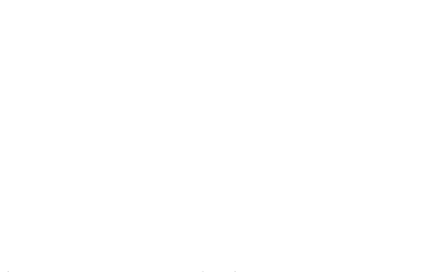
Figure 1: The two subsets $A_{\varepsilon}(x)$ and $A_{\varepsilon}(x^{\prime})$ for $\varepsilon=1/N$. The variance of the variables is given by the integral over $\theta(\mathrm{d}t,\mathrm{d}y)=y^{-2}\,\mathrm{d}t\,\mathrm{d}y$ of the lighter gray area above $\varepsilon=1/N$, and the covariance by the integral over the intersection of the subsets, the darker gray region.

The paper focuses on a discrete version of $\omega_{u}$. Let $N\in\mathbb{N}$, and take $\varepsilon=1/N$. Define the set

$$\mathcal{X}_{N}=\mathcal{X}_{\varepsilon}:=\biggl{\{}0,\frac{1}{N},\frac{2}{N},\ldots,\frac{i}{N},\ldots,\frac{N-1}{N}\biggr{\}}.$$

The notation $\mathcal{X}_{N}$ and $\mathcal{X}_{\varepsilon}$ will be used equally depending on the context. For a given $N$, the $\log$-correlated Gaussian field is the collection of Gaussian centered random variables $\omega_{\varepsilon}(x)$ for $x\in\mathcal{X}_{N}$,

$$X=(X_{x},x\in\mathcal{X}_{N})=\bigl{(}\omega_{\varepsilon}(x),x\in\mathcal{X}_{N}\bigr{)}.$$ (3)

A compelling feature of this construction is that a scale decomposition for $X$ is easily obtained from property (ii) above. Indeed, it suffices to write the variable $X_{x}$ as a sum of independent Gaussian fields corresponding to disjoint horizontal strips of $\mathcal{C}^{+}$. The $y$-axis then plays the role of the scale.

The covariances of the field are computed from (2) by straightforward integration; see also Figure 1.

Lemma 1.1

For any $0<\varepsilon=1/N<1/2$,

$$\mathbb{E}\bigl{[}X_{x}^{2}\bigr{]} = \sigma^{2}(\log N+1-\log 2),\qquad x\in\mathcal{X}_{N},$$

$$\mathbb{E}[X_{x}X_{x^{\prime}}] = \sigma^{2}\bigl{(}\log\bigl{(}1/\bigl{\|}x-x^{\prime}\bigr{\|}\bigr{)}-\log 2\bigr{)},\qquad x\neq x^{\prime}\in\mathcal{X}_{N}.$$

Similar constructions of log-correlated Gaussian fields using a random measure on cone-like subsets are also possible in two dimensions; see, for example, robert-vargas .

1.2 Main results

Without loss of generality, the results of this section are stated for the variance parameter $\sigma=1$. The points where the field is unusually high, the extremes or the high points, can be studied using a minor adaptation of the arguments of Daviaud for the two-dimensional discrete Gaussian free field daviaud . We denote by $|\mathcal{A}|$ the cardinality of a finite set $\mathcal{A}$.

Theorem 1.2 ((Daviaud daviaud ))

Let

$$\mathcal{H}_{N}(\gamma):=\{x\in\mathcal{X}_{N}\dvtx X_{x}\geq\sqrt{2}\gamma\log N\}$$

be the set of $\gamma$-high points. Then for any $0<\gamma<1$,

$$\lim_{N\to\infty}\frac{\log|\mathcal{H}_{N}(\gamma)|}{\log N}=1-\gamma^{2}\qquad\mbox{in probability.}$$

Moreover, for all $\rho>0$ there exists a constant $c=c(\rho)>0$ such that

$$\mathbb{P}\bigl{(}\bigl{|}\mathcal{H}_{N}(\gamma)\bigr{|}\leq N^{(1-\gamma^{2})-\rho}\bigr{)}\leq\exp\bigl{\{}-c(\log N)^{2}\bigr{\}}$$

for $N$ large enough.

The technique of Daviaud is based on a tree approximation introduced by Bolthausen, Deuschel and Giacomin bolthausen-deuschel-giacomin for the discrete two-dimensional Gaussian free field. There, the technique is used to obtain the first order of the maximum. The same argument applies here. Theorem 1.2 and simple Gaussian estimates yield

$$\lim_{N\to\infty}\frac{\max_{x\in\mathcal{X}_{N}}X_{x}}{\log N}=\sqrt{2}\qquad\mbox{a.s.}$$ (4)

The important feature of Theorem 1.2 and equation (4) is that they are identical to the results for $N$ i.i.d. Gaussian variables of variance $\log N$. In other words, the above observables of the high points are not affected by the correlations of the field. The i.i.d. case is called the random energy model (REM) in the spin glass literature.

The starting point of the paper is to understand to which extent i.i.d. statistics is a good approximation for more refined observables of the extremes of log-correlated Gaussian fields. To this end, we turn to tools of statistical physics which allow for a good control of the correlations.

First, consider the partition function $Z_{N}(\beta)$ of the model ($\beta$ stands for the inverse-temperature),

$$Z_{N}(\beta):=\sum_{x\in\mathcal{X}_{N}}\exp\{\beta X_{x}\}\qquad\forall\beta>0,$$

and the free energy

$$f_{N}(\beta):=\frac{1}{\log N}\log Z_{N}(\beta)\qquad\forall\beta>0.$$

Theorem 1.2 is used to compute the free energy of the model.

Corollary 1.3

Let $\beta_{c}:=\sqrt{2}$. Then, for all $\beta>0$

$$f(\beta):=\lim_{N\to\infty}f_{N}(\beta)=\cases{\displaystyle 1+\frac{\beta^{2}}{2},&\quad$\mbox{if }\beta<\beta_{c}$,\vspace*{2pt}\cr\sqrt{2}\beta,&\quad$\mbox{if }\beta\geq\beta_{c}$,}\qquad\mbox{a.s. and in $L^{1}$.}$$

The free energy is the same as for the REM with variance $\log N$. In particular, the model undergoes freezing above $\beta_{c}$ in the sense that the quantity $f(\beta)/\beta$ is constant.

More importantly, consider the normalized Gibbs weights or Gibbs measure

$$G_{\beta,N}(x):=\frac{\mathrm{e}^{\beta X_{x}}}{Z_{N}(\beta)},\qquad x\in\mathcal{X}_{N}.$$

By design, the Gibbs measure concentrates on the high points of the Gaussian field. The first main result of the paper is to achieve a control of the correlations at the level of the Gibbs measure. Precisely, with spin glasses in mind, we consider the normalized covariance or overlap

$$q(x,y)=q^{(N)}(x,y):=-\frac{\log\|y-x\|}{\log N},\qquad x,y\in\mathcal{X}_{N}.$$ (5)

Clearly, $\|x-y\|=\varepsilon^{q(x,y)}$ and $0\leq q(x,y)\leq 1$. Moreover, the overlap $q(x,y)$ is equal to the normalized correlations $\mathbb{E}[X_{x}X_{y}]/\mathbb{E}[X_{x}^{2}]$ plus a term that goes to zero as $N$ goes to infinity.

A fundamental object, that records the correlations of high points, is the distribution function of the overlap sampled from the Gibbs measure. Namely, denote by $G_{\beta,N}^{\times 2}$ the product measure on $\mathcal{X}_{N}\times\mathcal{X}_{N}$. Let $(x_{1},x_{2})\in\mathcal{X}_{N}^{2}$ be sampled from $G_{\beta,N}^{\times 2}$. Write for simplicity $q_{12}$ for $q(x_{1},x_{2})$. The averaged distribution function of the overlap is

$$x_{\beta}^{(N)}(q):={\mathbb{E}}\bigl{[}G_{\beta,N}^{\times 2}\{q_{12}\leq q\}\bigr{]},\qquad 0\leq q\leq 1.$$ (6)

The first result is the analogue of results of Derrida and Spohn for the Gibbs measure of branching Brownian motion (see equation (6.19) in derrida-spohn ), of Chauvin and Rouault on branching random walks chauvin-rouault and of Bovier and Kurkova on Derrida’s generalized random energy models (GREM) derrida , bovier-kurkova1 . It had been conjectured for nonhierarchical log-correlated Gaussian field by Carpentier and Le Doussal; see page 16 in carpentier-ledoussal .

Theorem 1.4

For $\beta>\beta_{c}$,

$$\lim_{N\to\infty}x_{\beta}^{(N)}(q)=\lim_{N\to\infty}{\mathbb{E}}\bigl{[}G_{\beta,N}^{\times 2}\{q_{12}\leq q\}\bigr{]}=\cases{\displaystyle\frac{\beta_{c}}{\beta},&\quad$\mbox{for $0\leq q<1$,}$\vspace*{2pt}\cr 1,&\quad$\mbox{for $q=1$.}$}$$

This result is the same as for the REM model talagrand . It is therefore consistent with rich statistics of extremes consisting of many high values order one away of each other and whose correlations are either very high or close to $0$. This result is in expectation. The typical behavior of the random variable $G_{\beta,N}^{{\times 2}}\{q_{12}\leq q\}$ for $q$ small in terms of $\beta$ should be exponentially small in $\beta$ rather than $1/\beta$. To see this, at the heuristic level, it is informative to consider the i.i.d. case where the same phenomenon occurs. Consider $N$ i.i.d. Gaussian random variables $(X_{i})_{1\leq i\leq N}$ of variance $\log N$ ordered in a decreasing way. In this case, $q_{ij}=0$ if $i\neq j$. The following inequality is easily verified:

$$G_{\beta,N}^{\times 2}\{q_{12}=0\}=\frac{\sum_{i\neq j}\mathrm{e}^{\beta X_{i}}\mathrm{e}^{\beta X_{j}}}{(\sum_{i}\mathrm{e}^{\beta X_{i}})^{2}}\leq 2\sum_{j\geq 2}\mathrm{e}^{\beta(X_{j}-X_{1})}.$$

In particular, since the gap $X_{1}-X_{2}$ is of order one in the limit and since the density of points at distance $x$ from the maximum is bounded by $\mathrm{e}^{Cx}$ for $C$ large enough (see bolthausen-sznitman for a precise statement in terms of extremal process), the typical behavior of $G_{\beta,N}^{{\times 2}}\{q_{12}=0\}$ is expected to be exponentially small in $\beta$.

We remark also that for $\beta\leq\beta_{c}$ the free energy contains all information about the two-overlap distribution. Indeed, since the free energy in Corollary 1.3 is differentiable for every $\beta>0$ including $\beta_{c}$, we have by the convexity of the free energy that the derivative of the limit is the limit of the derivatives. Hence

$$\lim_{N\to\infty}f^{\prime}_{N}(\beta)=\lim_{N\to\infty}\beta\bigl{(}1-\mathbb{E}G_{\beta,N}^{\times 2}[q_{12}]\bigr{)}=f^{\prime}(\beta).$$

The first equality is by Gaussian integration by part. It follows that$\lim_{N}\mathbb{E}[G_{\beta,N}^{\times 2}(q_{12})]=0$ for $\beta\leq\beta_{c}$. In particular, since the correlations are positive, the overlap of two sampled points is $0$ almost surely for every $\beta\leq\beta_{c}$.

In the case of $\beta>\beta_{c}$, the first moment of the two-overlap distribution is strictly greater than $0$, therefore more information is needed to determine the distribution. One way to proceed would be to obtain enough expectations of functions of $q_{12}$ to determine the distribution. This can be done by adding parameters to the field and consider the appropriate derivative of the free energy of the perturbed model. This is similar in spirit to the $p$-spin perturbations for the Sherrington–Kirkpatrick model in spin glasses; see, for example, talagrand . It turns out that this kind of pertubative approach pioneered by Bovier and Kurkova in bovier-kurkova2 for Gaussian fields on trees can be generalized to log-correlated fields. The control of the correlations is achieved by introducing a perturbed version of the model at a specific scale; cf. Section 2.1. In the present case, the proof is more intricate since the structure of correlations of the Gaussian field for finite $N$ is not tree-like or ultrametric as in the cases of branching Brownian motion and GREM’s. For example, for branching Brownian motion, $q(x,y)$ corresponds to the branching time of the common ancestor of two particles at time $t$, $x$ and $y$, divided by $t$. Because of the branching structure,

$$\qquad\mbox{the inequality }q(x,y)\geq\min\bigl{\{}q(x,z),q(y,z)\bigr{\}}\mbox{ is satisfied for all $x,y,z$.}$$ (7)

[The terminology ultrametric comes from the fact that the distance induced by the form $q(\cdot,\cdot)$ is ultrametric when (7) holds.]

The Parisi ultrametricity conjecture in the spin-glass literature states that, even though tree-like correlations might not be present for finite $N$, ultrametric correlations are recovered in the limit $N\to\infty$ for a large class of Gaussian fields at the level of the Gibbs measure, that is,

$$\lim_{N\to\infty}{\mathbb{E}}\bigl{[}G_{\beta,N}^{\times 3}\bigl{\{}q_{12}\geq\min\{q_{13},q_{23}\}\bigr{\}}\bigr{]}=1.$$ (8)

It is not hard to see that Theorem 1.4 implies the ultrametricity conjecture for the Gaussian field considered, since the overlaps can only take value $0$ or $1$. (In the language of spin glasses, the field is said to admit a one-step replica symmetry breaking at low temperature.)

The second main result describes the joint distribution of overlaps sampled from the Gibbs measure. To this end, for $s\geq 2$, we denote the product of Gibbs measure on $\mathcal{X}_{N}^{s}$ by $G_{\beta,N}^{\times s}$. We consider the class of continuous functions $F\dvtx[0,1]^{{s(s-1)}/{2}}\to\mathbb{R}$. We write $\mathbb{E}G_{\beta,N}^{\times s}[F(q_{ll^{\prime}})]$ for $\mathbb{E}G_{\beta,N}^{\times s}[F(\{q(x_{l},x_{l^{\prime}})\}_{1\leq l<l^{\prime}\leq s})]$, that is, the averaged expectation of $F(\{q(x_{l},x_{l^{\prime}})\}_{1\leq l<l^{\prime}\leq s})$ when $(x_{1},\ldots,x_{s})$ is sampled from $G_{\beta,N}^{\times s}$. We recall the definition of a Poisson–Dirichlet variable. For $0<\alpha<1$, let $\eta=(\eta_{i},i\in\mathbb{N})$ be the atoms of a Poisson random measure on $(0,\infty)$ of intensity measure $s^{-\alpha-1}\,\mathrm{d}s$. A Poisson–Dirichlet variable $\xi$ of parameter $\alpha$ is a random variable on the space of decreasing weights $\vec{s}=(s_{1},s_{2},\ldots)$ with $1\geq s_{1}\geq s_{2}\geq\cdots\geq 0$ and $\sum_{i}s_{i}\leq 1$ which has the same law as

$$\xi\,{\stackrel{{\scriptstyle\mathrm{law}}}{{=}}}\,\biggl{(}\frac{\eta_{i}}{\sum_{j}\eta_{j}},i\in\mathbb{N}\biggr{)}_{\downarrow},$$

where $\downarrow$ stands for the decreasing rearrangement.

Theorem 1.5

Let $\beta>\beta_{c}$ and $\xi=(\xi_{k},k\in\mathbb{N})$ be a Poisson–Dirichlet variable of parameter $\beta_{c}/\beta$. Denote by $E$ the expectation with respect to $\xi$. For any continuous function $F\dvtx[0,1]^{{s(s-1)}/{2}}\to\mathbb{R}$ of the overlaps of $s$ points,

$$\lim_{N\to\infty}{\mathbb{E}}G_{\beta,N}^{\times s}\bigl{[}F(q_{ll^{\prime}})\bigr{]}=E\biggl{[}\sum_{k_{1}\in\mathbb{N},\ldots,k_{s}\in\mathbb{N}}\xi_{k_{1}}\cdots\xi_{k_{s}}F(\delta_{k_{l}k_{l^{\prime}}})\biggr{]}.$$

It is important to stress that, as in the case of branching Brownian motion and unlike the REM, it is not the collection $(G_{\beta,N}(x),x\in\mathcal{X}_{N})_{\downarrow}$ per se that converges to a Poisson–Dirichlet variable. Rather, the result suggests that the Poisson–Dirichlet weights are formed by the sum of the Gibbs weights of high points that are arbitrarily close to each other because the continuity of the function $F$ naturally identifies points $x,y$ for which $q(x,y)$ tends to $1$ in the limit $N\to\infty$. In the theory of spin glasses, these clusters of high points are often called pure states. For more on the connection with spin glasses, the reader is referred to talagrand-pure where the pure states are constructed explicitly for mean-field models.

1.3 Relation to previous results

Bolthausen and Kistler have studied a family of models called generalized GREMs for which the correlations are not ultrametric bolthausen-kistler1 , bolthausen-kistler2 for finite $N$. By construction, the overlaps of these models can only take a finite number of values (uniformly in $N$, the number of variables). They compute the free energies and the Gibbs measure and prove the Parisi ultrametricity conjecture for these. Bovier and Kurkova bovier-kurkova1 , bovier-kurkova2 have obtained the distribution of the Gibbs measure for Gaussian fields, called the CREMs, where the values of the overlaps are not a priori restricted. Their analysis is restricted to models with ultrametric correlations and include the case of branching Brownian motion.

The works of Bolthausen, Deuschel and Zeitouni bolthausen-deuschel-zeitouni , Bramson and Zeitouni bramson-zeitouni and Ding ding establish the tightness of the recentered maximum of the two-dimensional discrete Gaussian free field. We expect that their method can be applied to the Gaussian field we consider.

We note that Fang and Zeitouni fang-zeitouni have studied a branching random walk model where the variance of the motion is time-dependent. This model is related to the simpler GREM model of spin glasses and to the CREM of Bovier and Kurkova. The family of log-correlated Gaussian fields introduced in Section 2.2 is akin to these hierarchical models, where the scale parameter replaces the time parameter.

2 Outline of the proof

The proof is split in three steps, and each can be adapted (with different correlation estimates) to other log-correlated Gaussian fields. The Gaussian field we study has a graphical representation of its correlations as well as no boundary effect which help in illustrating the method.

2.1 A family of perturbed models

In this section, we define a family of Gaussian fields for which the variance parameter $\sigma$ is scale-dependent. It can be seen as the GREM analogue for the nonhierarchical Gaussian field considered here. We restrict ourselves to the case where $\sigma$ takes two values, which is the one needed for the proof of Theorem 1.4. However, the construction and the results can hold for any finite number of values.

Fix $\varepsilon=1/N$. We introduce a scale (or time) parameter $t$ by defining for any $t\in[0,1]$,

$$X_{x}(t):=\omega_{\varepsilon^{t}}(x),\qquad x\in\mathcal{X}_{\varepsilon}.$$

Observe that for any fixed $x$, the process $(X_{x}(t))_{0\leq t\leq 1}$ has independent increments and is a martingale for the filtration $(\mathcal{F}_{\varepsilon^{t}},t\geq 0)$,

$$\mathbb{E}\bigl{[}X_{x}(t)|\mathcal{F}_{\varepsilon^{s}}\bigr{]}=X_{x}(s)\qquad\mbox{for $t>s$}.$$

This is a consequence of the defining property (ii) of the random measure $\mu$.

The parameters of the family of perturbed models are $\alpha$ where $0<\alpha<1$ and $\vec{\sigma}=(\sigma_{1},\sigma_{2})$ with $\sigma_{i}>0$, $i=1,2$. For the sake of clarity and to avoid repetitive trivial corrections, it is assumed throughout the paper that $N^{\alpha}$ and $N^{1-\alpha}$ are integers. The Gaussian field $Y^{(\vec{\sigma},\alpha)}(t)=(Y^{(\vec{\sigma},\alpha)}_{x}(t),x\in\mathcal{X}_{\varepsilon})$ is defined from the field $X$ as follows:

$$Y^{(\vec{\sigma},\alpha)}_{x}(t)=\cases{\sigma_{1}X_{x}(t),&\quad$\mbox{if }0<t\leq\alpha,$\vspace*{2pt}\cr\sigma_{1}X_{x}(\alpha)+\sigma_{2}\bigl{(}X_{x}(t)-X_{x}(\alpha)\bigr{)},&\quad$\mbox{if }\alpha<t\leq 1.$}$$ (9)

The construction is depicted in Figure 2. We write $Y^{(\vec{\sigma},\alpha)}$ for the field $(Y^{(\vec{\sigma},\alpha)}_{x}(1),x\in\mathcal{X}_{\varepsilon})$. The dependence on $\vec{\sigma}$ and $\alpha$ will sometimes be dropped in the notation of $Y$ for simplicity.

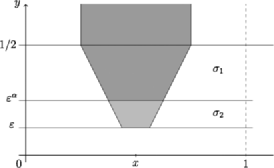
Figure 2: The cone associated with the process $Y_{x}(\cdot)$.

Consider the partition function $Z^{(\vec{\sigma},\alpha)}_{N}(\beta)$ of the perturbed model

$$Z_{N}^{(\vec{\sigma},\alpha)}(\beta):=\sum_{x\in\mathcal{X}_{N}}\exp(\beta Y_{x}),$$ (10)

and the free energy

$$f^{(\vec{\sigma},\alpha)}_{N}(\beta):=\frac{1}{\log N}\log Z_{N}^{(\vec{\sigma},\alpha)}(\beta)\qquad\forall\beta>0.$$

The log number of high points can be computed for the Gaussian field $Y$ using Daviaud’s technique recursively. The free energy is then obtained by doing an explicit sum on these high points. This is the object of Sections 3 and 4. The result is better expressed in terms of the free energy of the REM with $N$ i.i.d. Gaussian variables of variance $\sigma^{2}\log N$,

$$f\bigl{(}\beta;\sigma^{2}\bigr{)}:=\cases{\displaystyle 1+\frac{\beta^{2}\sigma^{2}}{2},&\quad$\mbox{if $\beta\leq\beta_{c}\bigl{(}\sigma^{2}\bigr{)}:=\displaystyle\frac{\sqrt{2}}{{\sigma}},$}$\vspace*{2pt}\cr\sqrt{2}\sigma\beta,&\quad$\mbox{if $\beta\geq\beta_{c}\bigl{(}\sigma^{2}\bigr{)}.$}$}$$

Corollary 1.3 follows from the next result with the choice $\sigma_{1}=\sigma_{2}$.

Proposition 2.1

Let $V_{12}:=\sigma_{1}^{2}\alpha+\sigma_{2}^{2}(1-\alpha)$. Then:

• Case 1: If $\sigma_{1}\leq\sigma_{2}$,

  $$\lim_{N\to\infty}f^{(\vec{\sigma},{\alpha})}_{N}(\beta)=f(\beta;V_{12}).$$

• Case 2: If $\sigma_{1}\geq\sigma_{2}$,

  $$\lim_{N\to\infty}f_{N}^{(\vec{\sigma},{\alpha})}(\beta)=\alpha f\bigl{(}\beta;\sigma_{1}^{2}\bigr{)}+(1-\alpha)f\bigl{(}\beta;\sigma_{2}^{2}\bigr{)},$$

where the convergence holds almost surely and in $L^{1}$.

The expressions are identical to the free energy of a GREM with two levels. In case 1, it is reduced to a REM. The conditions can be rewritten by defining a piecewise linear function of slopes $\sigma_{1}^{2}$ and $\sigma_{2}^{2}$ on the intervals $[0,\alpha]$, $[\alpha,1]$, respectively. In case 1, this function fails to be concave. However, it is easily verified that the effective parameters define the concave hull of the function. The reader is referred to capocaccia-cassandro-picco and bovier-kurkova1 for more details on the concavity conditions which is very general for the family of GREM models. In case 1 there is one critical value for $\beta$, and in case 2 there are two critical values for $\beta$ corresponding to the respective $\beta_{c}(\sigma^{2})$ of the two effective parameters $\sigma^{2}$. In case 1, the critical $\beta$ is $\sqrt{2/V_{12}}$, whereas the two critical $\beta$’s are $\sqrt{2}/\sigma_{1}$ and $\sqrt{2}/\sigma_{2}$ in case 2.

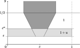
Figure 3: The perturbed model where the variance parameter is $(1+u)$ on the strip $[\varepsilon,\varepsilon^{\alpha}]$ where $\varepsilon=1/N$.

2.2 The Bovier–Kurkova technique

The proof of Theorem 1.4 relies on determining the overlap distribution of the original model from the free energy of the perturbed ones. This approach has been used by Bovier and Kurkova in the case of the GREM-type models bovier-kurkova1 , bovier-kurkova2 .

For $u\in(-1,1)$ and $\alpha\in(0,1)$, consider the field $(Y_{x},x\in\mathcal{X}_{\varepsilon})$ defined in (9) with the choice of parameters $\vec{\sigma}=(1,(1+u))$; see Figure 3. (Recall that, for the sake of clarity, it is assumed that $N^{\alpha}$ and $N^{1-\alpha}$ are integers.) The original Gaussian field $(X_{x})$ is recovered at $u=0$. Note that if $u>0$, the parameters correspond to the first case of Proposition 2.1 and if $u<0$, to the second. The field $Y$ can also be represented as follows:

$$Y_{x}=X_{x}+u\bigl{(}X_{x}-X_{x}(\alpha)\bigr{)},\qquad 1\leq i\leq N.$$ (11)

The proof of the next lemma is a simple integration and is postponed to the Appendix; see Appendix .2.

Lemma 2.2

Fix $0<\varepsilon=1/N<1/2$, and $\alpha\in(0,1)$. Let $\tilde{X}_{x}:=X_{x}-X_{x}(\alpha)$. Then, for $x\in\mathcal{X}_{\varepsilon}$

$$\mathbb{E}\bigl{[}\tilde{X}_{x}^{2}\bigr{]}=\mathbb{E}[\tilde{X}_{x}X_{x}]=(1-\alpha)\log N,\qquad x\in\mathcal{X}_{\varepsilon},$$

and, for $x,x^{\prime}\in\mathcal{X}_{\varepsilon}$,

$$\qquad\mathbb{E}[\tilde{X}_{x}X_{x^{\prime}}]=\cases{\bigl{(}q\bigl{(}x,x^{\prime}\bigr{)}-\alpha\bigr{)}\log N+O_{N}(1),&\quad$\mbox{if }\alpha<q\bigl{(}x,x^{\prime}\bigr{)}\leq 1,$\vspace*{2pt}\cr 0,&\quad$\mbox{if }0\leq q\bigl{(}x,x^{\prime}\bigr{)}\leq\alpha,$}$$ (12)

where $O_{N}(1)$ is a term uniformly bounded in $N$, and we recall that $\|x-x^{\prime}\|=\varepsilon^{q(x,x^{\prime})}$.

This result and a Gaussian integration by parts yield an important lemma.

Lemma 2.3

For all $\alpha\in(0,1)$, we have

$$\beta\int_{\alpha}^{1}x_{\beta}^{(N)}(s)\,\mathrm{d}s+o_{N}(1)=\frac{1}{\log N}{\mathbb{E}}\biggl{[}\sum_{x\in\mathcal{X}_{\varepsilon}}G_{\beta,N}(x)\bigl{(}X_{x}-X_{x}(\alpha)\bigr{)}\biggr{]},$$

where $o_{N}(1)$ stands for a term that goes to $0$ as $N$ goes to $\infty$.

Fix $\varepsilon=1/N$ and $\alpha\in(0,1)$. Note that $(\tilde{X}_{x};(X_{x^{\prime}},x^{\prime}\in\mathcal{X}_{\varepsilon}))$ is a Gaussian vector of $N+1$ variables. Therefore, Gaussian integration by parts (see Lemma .3) yields, for all $x\in\mathcal{X}_{\varepsilon}$,

$$\beta^{-1}{\mathbb{E}}\biggl{[}\frac{\tilde{X}_{x}\mathrm{e}^{\beta X_{x}}}{\sum_{x^{\prime}\in\mathcal{X}_{\varepsilon}}\mathrm{e}^{\beta X_{x^{\prime}}}}\biggr{]} = -\sum_{x^{\prime}\in\mathcal{X}_{\varepsilon}}{\mathbb{E}}[\tilde{X}_{x}X_{x^{\prime}}]{\mathbb{E}}\biggl{[}\frac{\mathrm{e}^{\beta(X_{x}+X_{x^{\prime}})}}{(\sum_{z\in\mathcal{X}_{\varepsilon}}\mathrm{e}^{\beta X_{z}})^{2}}\biggr{]}$$

$${}+{\mathbb{E}}[\tilde{X}_{x}X_{x}]{\mathbb{E}}\biggl{[}\frac{\mathrm{e}^{\beta X_{x}}}{\sum_{z\in\mathcal{X}_{\varepsilon}}\mathrm{e}^{\beta X_{z}}}\biggr{]}.$$

Lemma 2.2 and elementary manipulations imply

$$(\beta\log N)^{-1}{\mathbb{E}}\biggl{[}\sum_{x\in\mathcal{X}_{\varepsilon}}\tilde{X}_{x}G_{\beta,N}(x)\biggr{]}$$

$$\qquad=\sum_{x,x^{\prime}\in\mathcal{X}_{\varepsilon}}\biggl{(}\int_{\alpha}^{1}\mathbf{1}_{\{q(x,x^{\prime})\leq s\}}\,\mathrm{d}s\biggr{)}{\mathbb{E}}\bigl{[}G_{\beta,N}(x)G_{\beta,N}\bigl{(}x^{\prime}\bigr{)}\bigr{]}+O\biggl{(}\frac{1}{\log N}\biggr{)}$$

$$\qquad=\int_{\alpha}^{1}{\mathbb{E}}\bigl{[}G_{\beta,N}^{\times 2}\{q_{12}\leq s\}\bigr{]}\,\mathrm{d}s+O\biggl{(}\frac{1}{\log N}\biggr{)},$$

which concludes the proof of the lemma.

Proof of Theorem 1.4 Fix $\beta>\beta_{c}=\sqrt{2}$. Write $Z_{N}^{(u,\alpha)}(\beta)$ for the partition function (10) for the choice $\vec{\sigma}=(1,(1+u))$. Direct differentiation and equation (11) give

$$\frac{\mathrm{d}}{\mathrm{d}u}\bigl{(}{\mathbb{E}}\log Z_{N}^{(u,\alpha)}(\beta)\bigr{)}_{u=0}=\beta{\mathbb{E}}\biggl{[}\sum_{x\in\mathcal{X}_{\varepsilon}}\bigl{(}X_{x}-X_{x}(\alpha)\bigr{)}G_{\beta,N}(x)\biggr{]},$$

which, together with Lemma 2.3, yields

$$\int_{\alpha}^{1}x_{\beta}^{(N)}(s)\,\mathrm{d}s=\beta^{-2}(\log N)^{-1}\frac{\mathrm{d}}{\mathrm{d}u}\bigl{(}{\mathbb{E}}\log Z_{N}^{(u,\alpha)}(\beta)\bigr{)}_{u=0}+o_{N}(1).$$ (13)

Observe that ${\mathbb{E}}f_{N}^{(u,\alpha)}(\beta)=(\log N)^{-1}{\mathbb{E}}\log Z_{N}^{(u,\alpha)}(\beta)$ is a convex function of $u$. Moreover, by Proposition 2.1, ${\mathbb{E}}f_{N}^{(u,\alpha)}(\beta)$ converges. The limit, that we denote $f^{(u,\alpha)}(\beta)$, is also convex in the parameter $u$. In particular, by a standard result of convexity (see, e.g., Proposition I.3.2 in simon ), at every point of differentiability, the derivative of the limit equals the limit of the derivative

$$\lim_{N\to\infty}\frac{\mathrm{d}}{\mathrm{d}u}{\mathbb{E}}f_{N}^{(u,\alpha)}(\beta)=\frac{\mathrm{d}}{\mathrm{d}u}f^{(u,\alpha)}(\beta)$$

(14)

$$\eqntext{\mbox{$\forall u$ where $u\mapsto f^{(u,\alpha)}(\beta)$ is differentiable}.}$$ (15)

We show $f^{(u,\alpha)}(\beta)$ is differentiable at $u=0$. The derivative can be computed by Proposition 2.1. For $u$ small enough, $\beta$ is larger than all critical $\beta$’s. Thus

$$\frac{\mathrm{d}}{\mathrm{d}u}f^{(u,\alpha)}(\beta)=\cases{\displaystyle\sqrt{2}\beta\frac{(1-\alpha)(1+u)}{\sqrt{\alpha+(1-\alpha)(1+u)^{2}}},&\quad$\mbox{if }u>0,$\vspace*{2pt}\cr\sqrt{2}\beta(1-\alpha),&\quad$\mbox{if }u<0.$}$$ (16)

From this, it is easily verified that $f^{(u,\alpha)}(\beta)$ is differentiable at $u=0$ and

$$\frac{\mathrm{d}}{\mathrm{d}u}\bigl{(}f^{(u,\alpha)}(\beta)\bigr{)}_{u=0}=\sqrt{2}\beta(1-\alpha).$$ (17)

Equations (13), (2.2) and (17) together imply

$$\lim_{N\to\infty}\int_{\alpha}^{1}x^{(N)}_{\beta}(s)\,\mathrm{d}s=\frac{\sqrt{2}}{\beta}(1-\alpha)\qquad\mbox{for all $\alpha\in(0,1)$}.$$ (18)

Therefore, any weak limit $x_{\beta}$ must satisfy $x_{\beta}(\alpha)\leq\sqrt{2}/\beta$ for any point of continuity $\alpha<1$, since $x_{\beta}$ is nondecreasing. If there exists $0<\alpha<1$ such that $x_{\beta}(\alpha)<\frac{\sqrt{2}}{\beta}$, there would be a contradiction with (18), since by right-continuity and monotonicity of $x_{\beta}$ we could find $\alpha^{\prime}>\alpha$ such that

$$\lim_{N\to\infty}\int_{\alpha}^{\alpha^{\prime}}x^{(N)}_{\beta}(s)\,\mathrm{d}s<\frac{\sqrt{2}}{\beta}\bigl{(}\alpha^{\prime}-\alpha\bigr{)}.$$

This proves that any weak limit $x_{\beta}$ of $(x^{(N)}_{\beta},N\in\mathbb{N})$ is the same and equals $\frac{\sqrt{2}}{\beta}$ on $(0,1)$. The subsequential limits being the same, this proves in particular convergence of the sequence to the desired distribution function.

2.3 A spin-glass approach to Poisson–Dirichlet variables

In this section, the link between Theorems 1.4 and 1.5 is explained. The technique, inspired from the study of spin glasses in particular arguin-chatterjee , is general and is of independent interest to prove convergence to Poisson–Dirichlet statistics.

The first step is to find a good space for the convergence of $G_{\beta,N}$. Let $C$ be the compact metric space of $\mathbb{N}\times\mathbb{N}$ covariance matrices with $1$ on the diagonal endowed with the product topology on the entries. For a given $N$, consider the mapping

$$\mathcal{X}_{N}^{\times\infty} \to C,$$

$$(x_{l},l\in\mathbb{N}) \mapsto R^{(N)},$$

where for $l,l^{\prime}\in\mathbb{N}$

$$R^{(N)}_{l,l^{\prime}}:=\cases{q_{ll^{\prime}}=q\bigl{(}x_{l},x_{l}^{\prime}\bigr{)},&\quad$\mbox{if $l\neq l^{\prime}$}$\vspace*{2pt}\cr 1,&\quad$\mbox{if $l=l^{\prime}$.}$}$$

Consider the probability measure $\mathbb{E}G_{\beta,N}^{\times\infty}$ on $\mathcal{X}_{N}^{\times\infty}$. The push-forward of this probability measure under the above mapping defines a random element of $C$ that we denote $\vec{R}^{(N)}$. Since each point is sampled independently from the same measure, the law of $\vec{R}^{(N)}$ is weakly exchangeable, that is, for any permutation $\pi$ of a finite number of indices,

$$\bigl{(}\vec{R}^{(N)}_{\pi(l)\pi(l^{\prime})}\bigr{)}\,{\stackrel{{\scriptstyle\mathrm{law}}}{{=}}}\,\bigl{(}\vec{R}^{(N)}_{ll^{\prime}}\bigr{)}.$$

The sequence of random matrices $(\vec{R}^{(N)},N\in\mathbb{N})$ is tight by Prokhorov’s theorem since the space $C$ is a compact metric space. Hence, there exists a subsequence $\{\vec{R}^{(N_{m})}\}_{m\in\mathbb{N}}$ that converges weakly. Denote the subsequential limit by $\vec{R}$. Observe that $\vec{R}$ is also weakly exchangeable since the mappings on $C$ induced by a finite permutation is continuous. Therefore, by the representation theorem of Dovbysh and Sudakov dovbysh-sudakov , $\vec{R}$ is constructed like $\vec{R}^{(N)}$ by sampling from a random measure. Precisely, the theorem states that there exists a random probability measure $\mu_{\beta}$ on a Hilbert space $\mathcal{H}$, with law $P$ and corresponding expectation $E$, such that the random matrix $\vec{R}$ has the same law as the Gram matrix of a sequence of vectors $(v_{l},l\in\mathbb{N})$ that are sampled under $E\mu_{\beta}^{\times\infty}$. [In other words, the vectors $(v_{l},l\in\mathbb{N})$ are i.i.d. conditionally on $\mu_{\beta}$.] The equality in law can be expressed as follows: for any continuous function $F$ on $C$,

$$\lim_{m\to\infty}\mathbb{E}G_{\beta,N_{m}}^{\times\infty}\bigl{[}F(q_{ll^{\prime}})\bigr{]}=E\mu_{\beta}^{\times\infty}\bigl{[}F\bigl{(}v_{l}\cdot v_{l}^{\prime}\bigr{)}\bigr{]}.$$ (19)

Note that, since $q(x,x^{\prime})\leq 1$, the random measure $\mu_{\beta}$ is supported on the unit ball. The first consequence of Theorem 1.4 is that for any subsequential limit $\mu_{\beta}$,

$$E\bigl{[}\mu_{\beta}^{\times 2}\{v_{1}\cdot v_{2}\leq q\}\bigr{]} = \lim_{N\to\infty}{\mathbb{E}}\bigl{[}G_{\beta,N}^{\times 2}\{q_{12}\leq q\}\bigr{]}$$

$$= \frac{\beta_{c}}{\beta}1_{[0,1)}(q)+1_{\{1\}}(q).$$

The first equality is obtained by bounding $1_{[0,q]}(q_{ll^{\prime}})$ by continuous functions on $q_{ll^{\prime}}$ above and below and by applying (19). In view of equations (19) and (2.3), we see the random measures $\mu_{\beta}$ as limit points of $(G_{\beta,N})_{N\in\mathbb{N}}$.

The main ingredient to prove Poisson–Dirichlet statistics is a general property of the Gibbs measure $(G_{\beta,N}(x),x\in\mathcal{X}_{N})$ of centered Gaussian fields known as the Ghirlanda–Guerra identities. They were introduced in ghirlanda-guerra and were proved in a general setting by Panchenko panchenko_gg .

Theorem 2.4

Let $\mu_{\beta}$ be a subsequential limit of $(G_{\beta,N})_{N\in\mathbb{N}}$ inthe sense of (19). Then for any $s\in\mathbb{N}$ and any continuous functions $F\dvtx\break[-1,1]^{s(s-1)/2}\to\mathbb{R}$

$$E\mu_{\beta}^{\times s+1}\bigl{[}v_{1}\cdot v_{s+1}F(v_{l}\cdot v_{l^{\prime}})\bigr{]} = \frac{1}{s}E\mu_{\beta}^{\times 2}[v_{1}\cdot v_{2}]E\mu_{\beta}^{\times s}\bigl{[}F(v_{l}\cdot v_{l^{\prime}})\bigr{]}$$

$${}+\frac{1}{s}\sum_{k=2}^{s}E\mu_{\beta}^{\times s}\bigl{[}v_{1}\cdot v_{k}F(v_{l}\cdot v_{l^{\prime}})\bigr{]}.$$

Recall that we write $G_{\beta,N}^{\times s}$ for the product measure on $\mathcal{X}_{N}^{s}$. Also for $(x_{1},\ldots,x_{s})\in\mathcal{X}_{N}^{s}$, the overlaps $q(x_{l},x_{l}^{\prime})$, $1\leq l,l^{\prime}\leq s$, are denoted $q_{ll^{\prime}}$. In a similar way, we write $X_{1}$ for the field $X_{x_{1}}$ of the first point sampled from $G_{\beta,N}$. It is shown in panchenko_gg that, for any $\beta$ where the free energy $f(\beta)$ is differentiable, the following concentration holds:

$$\lim_{N\to\infty}\frac{1}{\log N}\mathbb{E}G_{\beta,N}\bigl{[}\bigl{|}X_{1}-\mathbb{E}G_{\beta,N}(X_{1})\bigr{|}\bigr{]}=0.$$ (22)

Note that by Corollary 1.3, differentiability holds at all $\beta$ for the Gaussian field considered. Since the function $F$ is bounded, (22) implies

$$\quad\lim_{N}\frac{1}{\log N}\bigl{(}\mathbb{E}G_{\beta,N}^{\times s}\bigl{[}X_{1}F(q_{ll^{\prime}})\bigr{]}-\mathbb{E}G_{\beta,N}[X_{1}]\mathbb{E}G_{\beta,N}^{\times s}\bigl{[}F(q_{ll^{\prime}})\bigr{]}\bigr{)}=0.$$ (23)

The two terms can be evaluated by Gaussian integrations by part (see Lemma .3),

$$\frac{1}{\beta\log N}\mathbb{E}G_{\beta,N}[X_{1}]=1-\mathbb{E}G_{\beta,N}^{\times 2}[q_{12}]+O\biggl{(}\frac{1}{\log N}\biggr{)}$$ (24)

and

$$\frac{1}{\beta\log N}\mathbb{E}G_{\beta,N}^{\times s}\bigl{[}X_{1}F(q_{ll^{\prime}})\bigr{]}$$

$$\qquad=-s\mathbb{E}G_{\beta,N}^{\times s+1}\bigl{[}q_{1,s+1}F(q_{ll^{\prime}})\bigr{]}+\sum_{1\leq k\leq s}\mathbb{E}G_{\beta,N}^{\times s}\bigl{[}q_{1k}F(q_{ll^{\prime}})\bigr{]}$$ (25)

$$\qquad\quad{}+O\biggl{(}\frac{1}{\log N}\biggr{)}.$$

Finally recalling (23) and assembling (24)–(2.3) yields the Ghirlanda–Guerra identities (see equation (16) in ghirlanda-guerra ),

$$\mathbb{E}G_{\beta,N}^{\times s+1}\bigl{[}q_{1,s+1}F(q_{ll^{\prime}})\bigr{]}$$

$$\qquad=\frac{1}{s}\mathbb{E}G_{\beta,N}^{\times 2}[q_{12}]\mathbb{E}G_{\beta,N}^{\times s}\bigl{[}F(q_{ll^{\prime}})\bigr{]}+\frac{1}{s}\sum_{k=2}^{s}\mathbb{E}G_{\beta,N}^{\times s}\bigl{[}q_{1k}F(q_{ll^{\prime}})\bigr{]}$$ (26)

$$\qquad\quad{}+o_{N}(1).$$

[Note that the term for $k=1$ cancels with the 1 since $q_{11}=1+o_{N}(1)$.] In particular, for any subsequential limit $\mu_{\beta}$ of $(G_{\beta,N})_{N}$ in the sense of (19), one obtains (2.4) by taking the limit $N\to\infty$ and applying the definition of convergence in the sense of (19).

Equation (2.3) and the Ghirlanda–Guerra identities imply that $\mu_{\beta}$ is atomic.

Corollary 2.5

Let $\mu_{\beta}$ be a subsequential limit of $(G_{\beta,N})_{N\in\mathbb{N}}$ in the sense of (19). Then there exist random weights $\xi=(\xi_{i};i\in\mathbb{N})_{\downarrow}$ with $\xi_{i}\geq 0$, $\sum_{i\in\mathbb{N}}\xi_{i}=1$ and orthonormal vectors $(e_{i};i\in\mathbb{N})\subset\mathcal{H}$ such that

$$\mu_{\beta}=\sum_{i\in\mathbb{N}}\xi_{i}\delta_{e_{i}},\qquad P\mbox{-a.s.}$$

Moreover, from (2.3), $E[\sum_{i\in\mathbb{N}}\xi_{i}^{2}]=1-\frac{\beta_{c}}{\beta}$.

Let $(v_{l},l\in\mathbb{N})$ be a sequence sampled from $E\mu_{\beta}^{\times\infty}$. From $(v_{l},l\in\mathbb{N})$, we reconstruct $\mu_{\beta}$ up to isometry. For a fixed $l$ consider the sequence $(v_{l}\cdot v_{l^{\prime}},l^{\prime}>l)$. This is a sequence of 0’s and 1’s by (2.3). We first show that, almost surely, for every $l\in\mathbb{N}$, there exists $l^{\prime}>l$ such that $v_{l}\cdot v_{l^{\prime}}=1$; in particular, since all vectors are in the unit ball, $v_{l}=v_{l^{\prime}}$ and $\|v_{l}\|=1$. For this, we proceed as in Lemma 1 in panchenko_gg2 . Write $F_{s}(v_{l}\cdot v_{l^{\prime}})=\prod_{l=2}^{s}(1-v_{1}\cdot v_{l})$. In other words, $F_{s}(v_{l}\cdot v_{l^{\prime}})$ is $1$ if $v_{1}\cdot v_{l}=0$ for $l=2,\ldots,s$, otherwise it is $0$. Denote for short $\alpha=1-E\mu_{\beta}^{\times 2}[v_{1}\cdot v_{2}]$. Equation (2.4) implies

$$E\mu_{\beta}^{\times s+1}\{v_{1}\cdot v_{l}=0,2\leq l\leq s+1\}$$

$$\qquad=E\mu_{\beta}^{\times s+1}\bigl{[}(1-v_{1}\cdot v_{s+1})F_{s}(v_{l}\cdot v_{l^{\prime}})\bigr{]}$$

$$\qquad=\frac{\alpha}{s}E\mu_{\beta}^{\times s}\{v_{1}\cdot v_{l}=0,2\leq l\leq s\}+\frac{1}{s}\sum_{l=2}^{s}E\mu_{\beta}^{\times s}\{v_{1}\cdot v_{l}=0,2\leq l\leq s\}$$

$$\qquad=\frac{s-1+\alpha}{s}E\mu_{\beta}^{\times s}\{v_{1}\cdot v_{l}=0,2\leq l\leq s\}=\frac{(s-1+\alpha)\cdots(1+\alpha)\alpha}{s!},$$

where the last equality is obtained by induction. The last term goes to $0$ as $s\to\infty$ since $\alpha<1$, hence

$$E\mu_{\beta}^{\times\infty}\{v_{1}\cdot v_{l}=0,l\geq 2\}=0,$$

from which we deduce that, $P$-a.s., $\mu_{\beta}^{\times\infty}\{v_{1}\cdot v_{l}=0,l\geq 2\}=0$ and then that, for $\mu_{\beta}$-almost all $v$,

$$\mu_{\beta}^{\times\infty}\{v\cdot v_{l}=0,l\geq 2\}=0.$$

Since the vectors $v_{l}$ are i.i.d. $\mu_{\beta}$-sampled, it follows that, $P$-a.s., for $\mu_{\beta}$-almost all $v$, $\mu_{\beta}(v\cdot v_{1}=0)<1$, thus $\mu_{\beta}(v\cdot v_{1}=1)>0$ as claimed.

By the reasoning above, a vector that is sampled once in $(v_{l},l\in\mathbb{N})$ is sampled infinitely many times $E\mu_{\beta}^{\times\infty}$-a.s. Moreover, since the vectors are conditionally i.i.d., for $l\in\mathbb{N}$, the following limit exists and must be nonzero:

$$\lim_{n\to\infty}\frac{1}{n}\sum_{j=l+1}^{l+n}1_{v_{l}}(v_{j})>0,\qquad\mbox{$E\mu_{\beta}^{\times\infty}$-a.s.}$$ (27)

In particular, every sampled vector $v_{l}$ is an atom a.s. and its weight is measurable with respect to $(v_{l},l\in\mathbb{N})$. Moreover, if $v_{l}\neq v_{l^{\prime}}$, then $v_{l}\cdot v_{l^{\prime}}=0$ $E\mu_{\beta}^{\times\infty}$-a.s. Therefore the atoms are orthogonal. It remains to consider the different atoms without repetitions and reorder the weights. Let $e_{1}=v_{1}$, $e_{2}=v_{l_{2}}$ where $l_{2}=\inf\{l\geq 1\dvtx v_{l}\cdot e_{1}=0\}$, $e_{3}=v_{l_{3}}$ where $l_{3}=\inf\{l\geq l_{2}\dvtx v_{l}\cdot e_{i}=0,i=1,2\}$ , and so forth. By construction, $(e_{j},j\geq 1)$ are orthonormal vectors. (The collection is not necessarily infinite at this point.) We can assign to each vector $e_{j}$ its weight $\mu_{\beta}(\{e_{j}\})$ by (27). The collection can then be ordered in decreasing order to get the result.

The fact that $E[\sum_{i\in\mathbb{N}}\xi_{i}^{2}]=1-\frac{\beta_{c}}{\beta}$ is straightforward from (2.3).

To finish the proof of Theorem 1.5, it remains to show that the random weights $\xi$ are distributed like a Poisson–Dirichlet variable of parameter $\frac{\beta_{c}}{\beta}$. In fact, the parameter is already determined by Corollary 2.5, since for a Poisson–Dirichlet variable $\xi^{\prime}$ of parameter $x$, $E[\sum_{k}(\xi_{k}^{\prime})^{2}]=1-x$ holds; see, for example, Corollary 2.2 in ruelle . This will also imply that for any converging sequence of $(G_{\beta,N})$ in the sense of (19), the limit is the same. In particular, it implies convergence of the whole sequence by compactness.

To prove the Poisson–Dirichlet statistics of the weights $\xi$, we use the following characterization theorem of the law; see talagrand , page 22 for details. Define for all $m\in\mathbb{N}$ the joint moments of the weights

$$S(n_{1},\ldots,n_{m})=E\sum_{k_{1},\ldots,k_{m}}\xi_{k_{1}}^{n_{1}}\cdots\xi_{k_{m}}^{n_{m}}\qquad\mbox{for $n_{1},\ldots,n_{m}\geq 1$}.$$ (28)

The collection of $S(n_{1},\ldots,n_{m})$, $m\in\mathbb{N}$, determines the law of a random mass-partition, that is, a random variable on ordered sequences $1\geq r_{1}\geq r_{2}\geq\cdots\geq 0$ with $\sum_{i\in\mathbb{N}}r_{i}\leq 1$. If $\xi$ is a Poisson–Dirichlet variable, it is shown in talagrand , Proposition 1.2.8, that the moments satisfy the recursion relations

$$\qquad S(n_{1}+1,\ldots,n_{m}) = \frac{S(2)}{s}S(n_{1},\ldots,n_{m})+\frac{n_{1}-1}{s}S(n_{1},\ldots,n_{m})$$

$${}+\sum_{2\leq l\leq m}\frac{n_{l}}{s}S(n_{1}+n_{l},n_{2},\ldots,n_{l-1},n_{l+1},\ldots,n_{m}),$$

where $s=n_{1}+\cdots+n_{m}$. It is not hard to verify that all moments $S(n_{1},\ldots,n_{m})$ (and thus the law of $\xi$) are determined by recursion from $S(2)$ and the identities (2.3).

It turns out that these identities are satisfied by $\xi$ defined by Theorem 2.4 and Corollary 2.5.

Theorem 2.6

Let $\xi$ be a random mass-partition satisfying the assumptions of Corollary 2.5. The moments $S(n_{1},\ldots,n_{m})$ of $\xi$ satisfy (2.3) for any $m\in\mathbb{N}$ and any $n_{1},\ldots,n_{m}\in\mathbb{N}$. In particular, $\xi$ has the law of a Poisson–Dirichlet variable of parameter $1-S(2)$.

To deduce (2.3) from (2.4), we follow talagrand , pages 24–25. The set $\{1,\ldots,s\}$ can be decomposed into the disjoint union of sets $I_{1},\ldots,I_{m}$ with $|I_{j}|=n_{j}$ for all $1\leq j\leq m$. Consider the functions $(F_{j})_{1\leq j\leq m}$ given by $F_{j}(\delta_{k_{l}k_{l^{\prime}}}):=\prod_{k_{l},k_{l^{\prime}}\in I_{j}}\delta_{k_{l}k_{l^{\prime}}}$ and define $F:=\prod_{1\leq j\leq m}F_{j}$. Then elementary manipulations imply (2.3). Note that the second term on the right-hand side of (2.4) yields the last two terms of (2.3).

3 High points of the perturbed models

In this section, the log-number of high points at a given level is computed for the perturbed models introduced in Section 2. The focus is on the Gaussian field introduced in Section 2.1, though the technique applies to any perturbed model with a finite number of parameters. The free energies of the models are computed in Section 4.

Let $Y=(Y_{x},x\in\mathcal{X}_{\varepsilon})$ be the Gaussian field introduced in Section 2.1. Recall the notation and the two choices of parameters in Proposition 2.1:

$$\mathit{Case}\ 1\dvtx\qquad\sigma_{1}\leq\sigma_{2};$$

(30)

$$\mathit{Case}\ 2\dvtx\qquad\sigma_{1}\geq\sigma_{2}.$$

Define also as before $V_{12}:=\sigma_{1}^{2}\alpha+\sigma_{2}^{2}(1-\alpha)$.

Proposition 3.1

$$\lim_{N\to\infty}\mathbb{P}\Bigl{(}\max_{x\in\mathcal{X}_{\varepsilon}}Y_{x}\geq\sqrt{2}\gamma_{\mathrm{max}}\log N\Bigr{)}=0,$$

where

$$\gamma_{\mathrm{max}}=\gamma_{\mathrm{max}}(\vec{\sigma},\alpha):=\cases{\sqrt{V_{12}},&\quad$\mbox{for case 1;}$\vspace*{2pt}\cr\sigma_{1}\alpha+\sigma_{2}(1-\alpha),&\quad$\mbox{for case 2.}$}$$

Proposition 3.2

Let $\mathcal{H}_{N}^{Y}(\gamma):=\{x\in\mathcal{X}_{\varepsilon}:Y_{x}\geq\sqrt{2}\gamma\log N\}$ be the set of $\gamma$-high points. Then, for all $0<\gamma<\gamma_{\mathrm{max}}$,

$$\lim_{N\to\infty}\frac{\log|\mathcal{H}_{N}^{Y}(\gamma)|}{\log N}=\mathcal{E}^{(\vec{\sigma},\alpha)}(\gamma)\qquad\mbox{in probability,}$$

where in case 1,

$$\mathcal{E}^{(\vec{\sigma},\alpha)}(\gamma):=1-\frac{\gamma^{2}}{V_{12}};$$

and in case 2,

$$\mathcal{E}^{(\vec{\sigma},\alpha)}(\gamma):=\cases{\displaystyle 1-\frac{\gamma^{2}}{V_{12}},&\quad$\mbox{if $\displaystyle\gamma<\frac{V_{12}}{\sigma_{1}}$}$,\vspace*{2pt}\cr\displaystyle(1-\alpha)-\frac{(\gamma-\sigma_{1}\alpha)^{2}}{\sigma_{2}^{2}(1-\alpha)},&\quad$\mbox{if $\displaystyle\gamma\geq\frac{V_{12}}{\sigma_{1}}$.}$}$$

Moreover, for any $\mathcal{E}<\mathcal{E}^{(\vec{\sigma},\alpha)}(\gamma)$, there exists $c$ such that

$$\mathbb{P}\bigl{(}\bigl{|}\mathcal{H}_{N}^{Y}(\gamma)\bigr{|}\leq N^{\mathcal{E}}\bigr{)}\leq\exp\bigl{\{}-c(\log N)^{2}\bigr{\}}.$$

3.1 Proof of Proposition 3.1

The proof of case 1 is by a union bound,

$$\mathbb{P}\Bigl{(}\max_{x\in\mathcal{X}_{\varepsilon}}Y_{x}\geq\sqrt{2}\gamma_{\mathrm{max}}\log N\Bigr{)}\leq N\mathbb{P}(Y_{x}\geq\sqrt{2}\gamma_{\mathrm{max}}\log N),$$

which goes to zero by a Gaussian estimate; see Lemma .1. For case 2, we construct a Gaussian field with hierarchical correlations that dominates $Y$ at the level of the covariances. The result will follow by comparison using Slepian’s lemma.

Notice that if $\varepsilon<\|x-x^{\prime}\|\leq\varepsilon^{\alpha}$, the corresponding cone-like sets for $Y_{x}$ and $Y_{x^{\prime}}$ in $\mathcal{C}^{+}$ intersect between the lines $y=\varepsilon$ and $y=\varepsilon^{\alpha}$. Therefore the covariance of the variables satisfies, writing $\ell:=\|x-x^{\prime}\|$,

$$\mathbb{E}[Y_{x}Y_{x^{\prime}}] = \sigma_{2}^{2}\int_{\ell}^{\varepsilon^{\alpha}}\frac{y-\ell}{y^{2}}\,\mathrm{d}y+\sigma_{1}^{2}\biggl{(}\int_{\varepsilon^{\alpha}}^{1/2}\frac{y-\ell}{y^{2}}\,\mathrm{d}y+\int_{1/2}^{\infty}\frac{1/2-\ell}{y^{2}}\,\mathrm{d}y\biggr{)}$$

$$\geq \sigma_{1}^{2}\biggl{(}\log\frac{1/2}{\varepsilon^{\alpha}}-1\biggr{)}.$$

By applying the same reasoning when $\varepsilon^{\alpha}<\|x-x^{\prime}\|\leq 1/2$, one obtains the following lower bound for the covariance:

$$\mathbb{E}[Y_{x}Y_{x^{\prime}}]\geq\cases{0,&\quad$\mbox{if $\bigl{\|}x-x^{\prime}\bigr{\|}>\varepsilon^{\alpha},$}$\vspace*{2pt}\cr\displaystyle\sigma_{1}^{2}\biggl{(}\log\frac{1/2}{\varepsilon^{\alpha}}-1\biggr{)},&\quad$\mbox{if $\varepsilon<\bigl{\|}x-x^{\prime}\bigr{\|}\leq\varepsilon^{\alpha}.$}$}$$ (31)

Equation (31) is used to construct a Gaussian field $\tilde{Y}$. Define the map

$$\pi\dvtx\mathcal{X}_{\varepsilon} \to \mathcal{X}_{\varepsilon^{\alpha}},$$

$$x \mapsto \pi(x),$$

where $\pi(x)$ is the unique $y\in\mathcal{X}_{\varepsilon^{\alpha}}$ such that $\|x-y\|\leq\frac{\varepsilon^{\alpha}}{2}$. (If $\|x-y\|=\frac{\varepsilon^{\alpha}}{2}$, there are two possibilities for $y$. We take the right point.) The pre-image of $y\in\mathcal{X}_{\varepsilon^{\alpha}}$ under $\pi$ are exactly the points in $\mathcal{X}_{\varepsilon}$ that are at a distance less than $\frac{\varepsilon^{\alpha}}{2}$ from $y$. One can think of $\pi(x)$ as the ancestor of $x$ at the scale $\varepsilon^{\alpha}$.

Consider the following Gaussian variables

$$\bigl{(}g^{(1)}_{x},x\in\mathcal{X}_{\varepsilon^{\alpha}}\bigr{)}\qquad\mbox{i.i.d. Gaussians of variance $\sigma_{1}^{2}\alpha\log N-\sigma_{1}^{2}\log 2-\sigma_{1}^{2}$,}$$

(32)

$$\bigl{(}g^{(2)}_{x},x\in\mathcal{X}_{\varepsilon}\bigr{)}\qquad\mbox{i.i.d. Gaussians of variance $\sigma_{2}^{2}(1-\alpha)\log N+2\sigma_{1}^{2}$.}$$

These two families are also assumed independent. Then, the field $\tilde{Y}$ is defined, using the map $\pi$ above and the Gaussian random variables $g_{x}^{(i)}$, by

$$\tilde{Y}_{x}=g_{\pi(x)}^{(1)}+g_{x}^{(2)}.$$ (33)

This construction and equation (31) directly imply the following comparison lemma.

Lemma 3.3

$$\mathbb{E}\bigl{[}\tilde{Y}_{x}^{2}\bigr{]} = \mathbb{E}\bigl{[}Y_{x}^{2}\bigr{]}\qquad\mbox{$\forall x\in\mathcal{X}_{\varepsilon}$},$$

$$\mathbb{E}[\tilde{Y}_{x}\tilde{Y}_{y}] \leq \mathbb{E}[Y_{x}Y_{y}]\qquad\mbox{$\forall$ $x\neq y$, $x,y\in\mathcal{X}_{\varepsilon}$.}$$

The following corollary is a straightforward consequence of the above lemma and Slepian’s lemma; see Corollary 3.12 in ledoux-talagrand .

Corollary 3.4

For any $\lambda>0$,

$$\mathbb{P}\Bigl{(}\max_{x\in\mathcal{X}_{\varepsilon}}Y_{x}\geq\lambda\Bigr{)}\leq\mathbb{P}\Bigl{(}\max_{x\in\mathcal{X}_{\varepsilon}}\tilde{Y}_{x}\geq\lambda\Bigr{)}.$$ (35)

The Gaussian field $\tilde{Y}$ is almost identical to a GREM model with two levels with parameters $0<\alpha<1$ and $\sigma_{1},\sigma_{2}$; see, for example, derrida , bovier-kurkova1 . In fact the only aspect different from an exact GREM are the terms of order one in the variances of the Gaussian random variables $g_{x}^{(i)}$’s. However, these do not affect the first order of the maximum. The proof of Proposition 3.1 is concluded by the following standard GREM result. The proof of the lemma is not hard and is omitted for conciseness. The reader is referred to Theorem 1.1 in bovier-kurkova1 where a stronger result on the maximum is given and to bolthausen-sznitman , Lecture 9, for more details on the free energy and on the log-number of high points of a two-level GREM.

Lemma 3.5

Let $\tilde{Y}$ be the Gaussian field constructed above. Then

$$\mathbb{P}\Bigl{(}\max_{x\in\mathcal{X}_{\varepsilon}}\tilde{Y}_{x}\geq\sqrt{2}\gamma_{\mathrm{max}}\log N\Bigr{)}\to 0,\qquad N\to\infty,$$

where $\gamma_{\mathrm{max}}$ is defined in Proposition 3.1.

3.1.1 Proof of the upper bound in Proposition 3.2

The goal is to get an upper bound in probability) for $|\mathcal{H}^{Y}_{N}(\gamma)|$ where $\mathcal{H}^{Y}_{N}(\gamma)=\{x\in\mathcal{X}_{\varepsilon}\dvtx Y_{x}\geq\sqrt{2}\gamma\log N\}$.

In case 1, a first moment computation gives the result. Indeed, a Gaussian estimate (see Lemma .1) gives

$$\mathbb{E}\bigl{[}\bigl{|}\mathcal{H}_{N}^{Y}(\gamma)\bigr{|}\bigr{]}=N\mathbb{P}(Y_{1}\geq\sqrt{2}\gamma\log N)\leq CN^{\mathcal{E}^{(\vec{\sigma},\alpha)}(\gamma)},$$

where $\mathcal{E}^{(\vec{\sigma},\alpha)}(\gamma)=1-\gamma^{2}/V_{12}$. Therefore, by Markov’s inequality, for any $\rho>0$,

$$\mathbb{P}\bigl{(}\bigl{|}\mathcal{H}_{N}^{Y}(\gamma)\bigr{|}\geq N^{\mathcal{E}^{(\vec{\sigma},\alpha)}(\gamma)+\rho}\bigr{)}\leq CN^{-\rho}\to 0,\qquad N\to 0.$$

In case 2, if $0<\gamma<V_{12}/\sigma_{1}=:\gamma_{\mathrm{crit}}$ the same argument gives the correct bound.

It remains to bound the case $\gamma\geq\gamma_{\mathrm{crit}}$. The argument is essentially an explicit comparison with a 2-level GREM. For the scale $\alpha$, define

$$\mathcal{H}_{N^{\alpha}}^{Y}(\gamma):=\bigl{\{}x\in\mathcal{X}_{\varepsilon^{\alpha}}\dvtx Y_{x}(\alpha)\geq\sqrt{2}\gamma\log N\bigr{\}},\qquad\mathcal{E}_{1}(\gamma):=\alpha-\frac{\gamma^{2}}{\sigma_{1}^{2}\alpha}.$$

A first moment computation yields, for any $0<\gamma_{1}<\sigma_{1}\alpha$ and any $\rho>0$,

$$\mathbb{P}\bigl{(}\bigl{|}\mathcal{H}_{N^{\alpha}}^{Y}(\gamma_{1})\bigr{|}\geq N^{\mathcal{E}_{1}(\gamma_{1})+\rho}\bigr{)}\leq CN^{-\rho}\to 0,\qquad N\to 0.$$ (36)

Similarly, a union bound gives

$$\mathbb{P}\Bigl{(}\max_{x\in\mathcal{X}_{\varepsilon^{\alpha}}}Y_{x}(\alpha)\geq\sqrt{2}\sigma_{1}\alpha\log N\Bigr{)}\to 0.$$ (37)

Recall that, for any $x\in\mathcal{X}_{\varepsilon}$, we denote by $\pi(x)$ the closest point in $\mathcal{X}_{\varepsilon^{\alpha}}$, hence $\|x-\pi(x)\|\leq\varepsilon^{\alpha}/2$. We define for all $N$ and $\nu>0$,

$$A_{N,\nu}:=\bigcup_{x\in\mathcal{X}_{\varepsilon}}\bigl{\{}\bigl{|}Y_{x}(\alpha)-Y_{\pi(x)}(\alpha)\bigr{|}\geq\nu\log N\bigr{\}}.$$

The parameter $\nu$ will be fixed later and will depend on $\rho$. Using a union bound together with Lemma .4, we obtain, for all $\nu>0$,

$$\mathbb{P}(A_{N,\nu})\leq CN\mathrm{e}^{-c(\log N)^{2}}\to 0,\qquad N\to 0.$$ (38)

We also consider the events giving the log-number of high points at scale $\alpha$. Precisely, we divide $[0,\sigma_{1}\alpha]$ in intervals of size $\sigma_{1}\alpha/M$ where $M$ will be fixed later. Define $\eta_{i}:=i\sigma_{1}\alpha/M$, for $0\leq i\leq M$ and

$$I^{(i)}:=[\sqrt{2}\eta_{i-1}\log N;\sqrt{2}\eta_{i}\log N],\qquad 1\leq i\leq M.$$

By (36), the events

$$B_{N,i}:=\bigl{\{}\bigl{|}\mathcal{H}_{N^{\alpha}}^{Y}(\eta_{i-1})\bigr{|}\geq N^{\mathcal{E}_{1}(\eta_{i-1})+\rho/2}\bigr{\}},\qquad 1\leq i\leq M$$

are such that

$$\mathbb{P}\Biggl{(}\bigcup_{i=1}^{M}B_{N,i}\Biggr{)}\to 0,\qquad N\to 0.$$ (39)

Therefore, by (38) and (39), we are reduced to estimate

$$\mathbb{P}\Biggl{(}\bigl{\{}\bigl{|}\mathcal{H}_{N}^{Y}(\gamma)\bigr{|}\geq N^{\mathcal{E}^{(\vec{\sigma},\alpha)}(\gamma)+\rho}\bigr{\}}\cap A_{N,\nu}^{c}\cap\bigcap_{i=1}^{M}B_{N,i}^{c}\Biggr{)},$$

which is smaller than

$$\frac{1}{N^{\mathcal{E}^{(\vec{\sigma},\alpha)}(\gamma)+\rho}}\mathbb{E}\Biggl{[}\bigl{|}\mathcal{H}_{N}^{Y}(\gamma)\bigr{|};A_{N,\nu}^{c},\bigcap_{i=1}^{M}B_{N,i}^{c}\Biggr{]}.$$ (40)

We split the set $\mathcal{H}_{N}^{Y}(\gamma)$ into the possible value of the field at scale $\alpha$

$$\mathcal{H}^{(i)}_{N}(\gamma) := \bigl{\{}x\in\mathcal{X}_{\varepsilon}\dvtx Y_{x}\geq\sqrt{2}\gamma\log N;Y_{\pi(x)}(\alpha)\in I^{(i)}\bigr{\}},\qquad 1\leq i\leq M,$$

$$\mathcal{H}^{(0)}_{N}(\gamma) := \bigl{\{}x\in\mathcal{X}_{\varepsilon}\dvtx Y_{x}\geq\sqrt{2}\gamma\log N;Y_{\pi(x)}(\alpha)\leq 0\bigr{\}}.$$

The term in (40) can then be bounded above by

$$\frac{1}{N^{\mathcal{E}^{(\vec{\sigma},\alpha)}(\gamma)+\rho}}\sum_{i=0}^{M}\mathbb{E}\bigl{[}\bigl{|}\mathcal{H}^{(i)}_{N}(\gamma)\bigr{|};A_{N,\nu}^{c}\cap B_{N,i}^{c}\bigr{]}.$$

If $0\leq\gamma\leq\gamma_{\mathrm{max}}$, note that $\mathcal{E}^{(\vec{\sigma},\alpha)}(\gamma)$ satisfies $\mathcal{E}^{(\vec{\sigma},\alpha)}(\gamma)=\max_{0\leq\eta\leq\sigma_{1}\alpha}Q(\eta)$ where

$$Q(\eta):=1-\frac{\eta^{2}}{\sigma_{1}^{2}\alpha}-\frac{(\gamma-\eta)^{2}}{\sigma_{2}^{2}(1-\alpha)}.$$

Moreover, if $\gamma_{\mathrm{crit}}\leq\gamma\leq\gamma_{\mathrm{max}}$, the maximum is attained at $\eta=\sigma_{1}\alpha$, thus $Q(\eta)\leq\mathcal{E}^{(\vec{\sigma},\alpha)}(\gamma)$ for all $\eta\in[0,\sigma_{1}\alpha]$. For $1\leq i\leq M$, one gets

$$\mathbb{E}\bigl{[}\bigl{|}\mathcal{H}^{(i)}_{N}(\gamma)\bigr{|};A_{N,\nu}^{c}\cap B_{N,i}^{c}\bigr{]}$$

$$\qquad=\mathbb{E}\biggl{[}\sum_{x\in\mathcal{X}_{\varepsilon}}\mathbf{1}_{\{Y_{x}\geq\sqrt{2}\gamma\log N,Y_{\pi(x)}(\alpha)\in I^{(i)}\}};A_{N,\nu}^{c}\cap B_{N,i}^{c}\biggr{]}$$

$$\qquad\leq\mathbb{E}\biggl{[}\sum_{x\in\mathcal{X}_{\varepsilon}}\mathbf{1}_{\{Y_{x}-Y_{x}(\alpha)\geq\sqrt{2}(\gamma-\eta_{i}-\nu)\log N,Y_{\pi(x)}(\alpha)\geq\sqrt{2}\eta_{i-1}\log N\}};B_{N,i}^{c}\biggr{]}$$

$$\qquad\leq CN^{\mathcal{E}_{1}(\eta_{i-1})+\rho/2}N^{1-\alpha}N^{-{(\gamma-\eta_{i}-\nu)^{2}}/{(\sigma_{2}^{2}(1-\alpha))}}$$

$$\qquad=CN^{\rho/2}N^{1-{(\eta_{i-1})^{2}}/{(\sigma_{1}^{2}\alpha)}-{(\gamma-\eta_{i}-\nu)^{2}}/{(\sigma_{2}^{2}(1-\alpha))}},$$

where the last inequality follows by the definition of $B_{N,i}$ the independence of the field at different scales and a Gaussian estimate. Since $Q(\eta)\leq\mathcal{E}^{(\vec{\sigma},\alpha)}(\gamma)$ for all $\eta\in[0,\sigma_{1}\alpha]$, the last term is smaller than $CN^{\mathcal{E}^{(\vec{\sigma},\alpha)}(\gamma)+3\rho/4}$ by taking $\nu$ small enough and $M$ large enough, but fixed. For $i=0$, a similar argument gives also the bound $CN^{\mathcal{E}^{(\vec{\sigma},\alpha)}(\gamma)+\rho/2}$. Putting this back in (40) shows that the term goes to $0$ as $N\to\infty$ as desired.

3.1.2 Proof of the lower bound in Proposition 3.2

The proof of the lower bound is two-step recursion. Two lemmas are needed. The first is a generalization of the lower bound in Daviaud’s theorem; see Theorem 1.2 or daviaud .

Lemma 3.6

Let $0<\alpha^{\prime}<\alpha^{\prime\prime}\leq 1$. Suppose that the parameter $\sigma$ is constant on the strip $[0,1]_{\sim}\times[\varepsilon^{\alpha^{\prime\prime}},\varepsilon^{\alpha^{\prime}}]$, and that the event

$$\Xi:=\bigl{\{}\#\bigl{\{}x\in\mathcal{X}_{\varepsilon^{\alpha^{\prime}}}\dvtx Y_{x}\bigl{(}\alpha^{\prime}\bigr{)}\geq\sqrt{2}\gamma^{\prime}\log N\bigr{\}}\geq N^{\mathcal{E}^{\prime}}\bigr{\}}$$

is such that

$$\mathbb{P}\bigl{(}\Xi^{c}\bigr{)}\leq\exp\bigl{\{}-c^{\prime}(\log N)^{2}\bigr{\}}$$

for some $\gamma^{\prime}\geq 0$, $\mathcal{E}^{\prime}>0$ and $c^{\prime}>0$.

Let

$$\mathcal{E}(\gamma):=\mathcal{E}^{\prime}+\bigl{(}\alpha^{\prime\prime}-\alpha^{\prime}\bigr{)}-\frac{(\gamma-\gamma^{\prime})^{2}}{\sigma^{2}(\alpha^{\prime\prime}-\alpha^{\prime})}>0.$$

Then, for any $\gamma^{\prime\prime}$ such that $\mathcal{E}(\gamma^{\prime\prime})>0$ and any $\mathcal{E}<\mathcal{E}(\gamma^{\prime\prime})$, there exists $c$ such that

$$\mathbb{P}\bigl{(}\#\bigl{\{}x\in\mathcal{X}_{\varepsilon^{\alpha^{\prime\prime}}}\dvtx Y_{x}\bigl{(}\alpha^{\prime\prime}\bigr{)}\geq\sqrt{2}\gamma^{\prime\prime}\log N\bigr{\}}\leq N^{\mathcal{E}}\bigr{)}\leq\exp\bigl{\{}-c(\log N)^{2}\bigr{\}}.$$

We stress that $\gamma^{\prime\prime}$ may be such that $\mathcal{E}(\gamma^{\prime\prime})<\mathcal{E}^{\prime}$. The second lemma, which follows, serves as the starting point of the recursion and is analogous to Lemma 8 in bolthausen-deuschel-giacomin .

Lemma 3.7

For any $\alpha_{0}$ such that $0<\alpha_{0}<\alpha$, there exists $\mathcal{E}_{0}=\mathcal{E}_{0}(\alpha_{0})>0$ and $c=c(\alpha_{0})$ such that

$$\mathbb{P}\bigl{(}\#\bigl{\{}x\in\mathcal{X}_{\varepsilon^{\alpha_{0}}}\dvtx Y_{x}(\alpha_{0})\geq 0\bigr{\}}\leq N^{\mathcal{E}_{0}}\bigr{)}\leq\exp\bigl{\{}-c(\log N)^{2}\bigr{\}}.$$

We first conclude the proof of the lower bound in Proposition 3.2 using the two above lemmas.

Proof of the lower bound of Proposition 3.2 Let $\gamma$ such that $0<\gamma<\gamma_{\mathrm{max}}$. Choose $\mathcal{E}$ such that $\mathcal{E}<\mathcal{E}^{(\vec{\sigma},\alpha)}(\gamma)$. It will be shown that for some $c>0$

$$\mathbb{P}\bigl{(}\bigl{|}\mathcal{H}_{N}^{Y}(\gamma)\bigr{|}\leq N^{\varepsilon}\bigr{)}\leq\exp\bigl{\{}-c(\log N)^{2}\bigr{\}}.$$ (41)

By Lemma 3.7, for $\alpha_{0}<\alpha$ arbitrarily close to $0$, there exists $\mathcal{E}_{0}=\mathcal{E}_{0}(\alpha_{0})>0$ and $c_{0}=c_{0}(\alpha_{0})>0$, such that

$$\mathbb{P}\bigl{(}\#\bigl{\{}x\in\mathcal{X}_{\varepsilon^{\alpha_{0}}}\dvtx Y_{x}(\alpha_{0})\geq 0\bigr{\}}\leq N^{\mathcal{E}_{0}}\bigr{)}\leq\exp\bigl{\{}-c_{0}(\log N)^{2}\bigr{\}}.$$ (42)

Observe that we have $0\leq\mathcal{E}_{0}\leq\alpha_{0}$. Moreover, let

$$\mathcal{E}_{1}(\gamma_{1}):=\mathcal{E}_{0}+(\alpha-\alpha_{0})-\frac{\gamma_{1}^{2}}{\sigma_{1}^{2}(\alpha-\alpha_{0})}.$$ (43)

Lemma 3.6 is applied from $\alpha_{0}$ to $\alpha$. For any $\gamma_{1}$ with $\mathcal{E}_{1}(\gamma_{1})>0$ and any $\mathcal{E}_{1}<\mathcal{E}_{1}(\gamma_{1})$, there exists $c_{1}>0$ such that

$$\mathbb{P}\bigl{(}\#\bigl{\{}x\in\mathcal{X}_{\varepsilon^{\alpha}}\dvtx Y_{x}(\alpha)\geq\sqrt{2}\gamma_{1}\log N\bigr{\}}\leq N^{\mathcal{E}_{1}}\bigr{)}\leq\exp\bigl{\{}-c_{1}(\log N)^{2}\bigr{\}}.$$

Therefore, Lemma 3.6 can be applied from $\alpha$ to $1$ for any $\gamma_{1}$ with $\mathcal{E}_{1}(\gamma_{1})>0$. Define similarly

$$\mathcal{E}_{2}(\gamma_{1},\gamma_{2}):=\mathcal{E}_{1}(\gamma_{1})+(1-\alpha)-\frac{(\gamma_{2}-\gamma_{1})^{2}}{\sigma_{2}^{2}(1-\alpha)}.$$ (44)

Then, for any $\gamma_{2}$ with $\mathcal{E}_{2}(\gamma_{1},\gamma_{2})>0$ and $\mathcal{E}_{2}<\mathcal{E}_{2}(\gamma_{1},\gamma_{2})$, there exists $c_{2}>0$ such that

$$\mathbb{P}\bigl{(}\#\{x\in\mathcal{X}_{\varepsilon}\dvtx Y_{x}\geq\sqrt{2}\gamma_{2}\log N\}\leq N^{\mathcal{E}_{2}}\bigr{)}\leq\exp\bigl{\{}-c_{2}(\log N)^{2}\bigr{\}}.$$ (45)

Recalling that $0\leq\mathcal{E}_{0}\leq\alpha_{0}$, equation (41) follows from (45) if it is proved that $\lim_{\alpha_{0}\to 0}\mathcal{E}_{2}(\gamma_{1},\gamma)=\mathcal{E}^{(\vec{\sigma},{\alpha})}(\gamma)$ for an appropriate choice of $\gamma_{1}$ [in particular such that $\mathcal{E}_{1}(\gamma_{1})>0$]. It is easily verified that, for a given $\gamma$, the quantity $\mathcal{E}_{2}(\gamma_{1},\gamma)$ is maximized at

$$\gamma_{1}^{*}=\gamma\frac{\sigma_{1}^{2}(\alpha-\alpha_{0})}{V_{12}-\sigma_{1}^{2}\alpha_{0}}.$$

Plugging these back in (43) shows that $\mathcal{E}_{1}(\gamma_{1}^{*})>0$ provided that

$$\gamma<\frac{V_{12}}{\sigma_{1}}=:\gamma_{\mathrm{crit}},$$

with $\alpha_{0}$ small enough (depending on $\gamma$). Furthermore, since

$$\mathcal{E}_{2}\bigl{(}\gamma_{1}^{*},\gamma\bigr{)}=\mathcal{E}_{0}+(1-\alpha_{0})-\frac{\gamma^{2}}{V_{12}-\sigma_{1}^{2}\alpha_{0}},$$

we obtain $\lim_{\alpha_{0}\to 0}\mathcal{E}_{2}(\gamma_{1}^{*},\gamma)=\mathcal{E}^{(\vec{\sigma},{\alpha})}(\gamma)$, which completes the proof in the case $0<\gamma<\gamma_{\mathrm{crit}}$.

If $\gamma_{\mathrm{crit}}\leq\gamma<\gamma_{\mathrm{max}}$, the condition $\mathcal{E}_{1}(\gamma_{1}^{*})>0$ will be violated as $\alpha_{0}$ goes to zero. In this case, for $\nu>0$, pick $\gamma_{1}^{**}=\sigma_{1}\alpha-\nu$ such that $\mathcal{E}_{1}(\gamma_{1}^{**})>0$. The first term in $\gamma_{1}^{**}$ corresponds to $\gamma_{1}^{*}$ evaluated at $\gamma_{\mathrm{crit}}$ for $\alpha_{0}=0$. In particular, $\lim_{\alpha_{0}\to 0,\nu\to 0}\mathcal{E}_{1}(\gamma_{1}^{**})=0$. From (44), this shows that

$$\lim_{\alpha_{0}\to 0,\nu\to 0}\mathcal{E}_{2}\bigl{(}\gamma_{1}^{**},\gamma\bigr{)}=(1-\alpha)-\frac{(\gamma-\sigma_{1}\alpha)^{2}}{\sigma_{2}^{2}(1-\alpha)}=\mathcal{E}^{(\vec{\sigma},{\alpha})}(\gamma).$$

Note that $\mathcal{E}^{(\vec{\sigma},{\alpha})}(\gamma)$ is strictly positive if and only if $\gamma<\sigma_{1}\alpha+\sigma_{2}(1-\alpha)=\gamma_{\mathrm{max}}$. This concludes the proof of (41).

Proof of Lemma 3.6 Let $\gamma^{\prime\prime}$ such that $\mathcal{E}(\gamma^{\prime\prime})>0$ and $\mathcal{E}$ such that $0<\mathcal{E}<\mathcal{E}(\gamma^{\prime\prime})$. Pick $\overline{\gamma}>\gamma^{\prime\prime}$ such that

$$\mathcal{E}(\overline{\gamma})>\mathcal{E}>0.$$ (46)

Since $\overline{\gamma}>\gamma^{\prime\prime}$, there exists $\varsigma\in(0,1)$ such that

$$\overline{\gamma}(1-\varsigma)\geq\gamma^{\prime\prime}.$$ (47)

For $K\in{\mathbb{N}}$ (which will be fixed later), we set

$$\eta_{\ell} := \alpha^{\prime}+\frac{\ell-1}{K}\bigl{(}\alpha^{\prime\prime}-\alpha^{\prime}\bigr{)},\qquad 1\leq\ell\leq K+1,$$

$$\lambda_{\ell} := \gamma^{\prime}+\frac{\ell-1}{K}\bigl{(}\overline{\gamma}-\gamma^{\prime}\bigr{)}(1-\varsigma),\qquad 1\leq\ell\leq K+1.$$

Observe that the $\eta_{\ell}$’s and the $\lambda_{\ell}$’s satisfy $\eta_{1}=\alpha^{\prime}<\eta_{2}<\cdots<\eta_{K}<\eta_{K+1}=\alpha^{\prime\prime}$, and $\lambda_{1}=\gamma^{\prime}<\lambda_{2}<\cdots<\lambda_{K}<\lambda_{K+1}=(1-\varsigma)\overline{\gamma}+\varsigma\gamma^{\prime}$. Consider the sets $\mathcal{A}_{\ell}$ given by

$$\mathcal{A}_{\ell}:=\bigl{\{}\underline{x}^{(\ell)}=(x_{1},\ldots,x_{\ell})\dvtx x_{i}\in\mathcal{X}_{2\varepsilon^{\eta_{i}}},\forall 1\leq i\leq\ell\mbox{ and }\|x_{i+1}-x_{i}\|\leq\varepsilon^{\eta_{i}}/2\bigr{\}}$$

for $1\leq\ell\leq K+1$. Note that only half of the $x_{i}$’s in $\mathcal{X}_{\varepsilon^{\eta_{i}}}$’s are considered. Also, to each $x_{i}$ we consider the points $x_{i+1}$ in $\mathcal{X}_{2\varepsilon^{\eta_{i+1}}}$ that are close to $x_{i}$. By analogy with a branching process, these points can be thought of as the children of $x_{i}$. The reason for these two choices is that the cones corresponding to the variables $Y_{x_{i+1}}(\eta_{i+1})$ and $Y_{x^{\prime}_{i+1}}(\eta_{i+1})$ do not intersect below the line $y=\varepsilon^{\eta_{i}}$ if $x_{i}\neq x_{i}^{\prime}$; see Figure 4.

Figure 4: Approximation by a tree-like structure. The black circles symbolize the children of the white circle, while the black squares symbolize the children of the white square.

Now consider, the sets of high points of $\mathcal{A}_{\ell}$,

$$A_{\ell}:=\bigl{\{}\underline{x}^{(\ell)}\in\mathcal{A}_{\ell}\dvtx Y_{x_{i}}(\eta_{i})\geq\sqrt{2}\lambda_{i}\log N,\forall 1\leq i\leq\ell\bigr{\}},\qquad 1\leq\ell\leq K+1$$

and

$$B_{\ell}:=\{\#A_{\ell}\geq n_{\ell}\},\qquad 1\leq\ell\leq K+1,$$

where

$$\qquad n_{\ell}:=N^{\mathcal{E}^{\prime}+{(\ell-1)}/{K}((\alpha^{\prime\prime}-\alpha^{\prime})-({(\overline{\gamma}-\gamma^{\prime})^{2}}/{(\sigma^{2}(\alpha^{\prime\prime}-\alpha^{\prime}))}))},\qquad 1\leq\ell\leq K+1,$$ (48)

such that $N^{\mathcal{E}^{\prime}}=n_{1}$ and $n_{K+1}=N^{\mathcal{E}(\overline{\gamma})}$. Furthermore, with these definitions and the choice of $\overline{\gamma}$ in (47) and (46), we have for large $N$

$$B_{K+1} = \{\#A_{K+1}>n_{{K+1}}\}$$

$${}\subset\bigl{\{}\#\bigl{\{}x\in\mathcal{X}_{\varepsilon^{\alpha^{\prime\prime}}}\dvtx Y_{x}\bigl{(}\alpha^{\prime\prime}\bigr{)}\geq\sqrt{2}\bigl{(}(1-\varsigma)\overline{\gamma}+\varsigma\gamma^{\prime}\bigr{)}\log N\bigr{\}}>N^{\mathcal{E}(\overline{\gamma})}\bigr{\}}$$

$${}\subset\bigl{\{}\#\bigl{\{}x\in\mathcal{X}_{\varepsilon^{\alpha^{\prime\prime}}}\dvtx Y_{x}\bigl{(}\alpha^{\prime\prime}\bigr{)}\geq\sqrt{2}\gamma^{\prime\prime}\log N\bigr{\}}>N^{\mathcal{E}}\bigr{\}}.$$

It is thus sufficient to find a bound for $\mathbb{P}(B_{K+1}^{c})$ to prove the lemma. For events $C_{\ell}$ to be defined in (3.1.2), we use the elementary bound $\mathbb{P}(B_{K+1}^{c})\leq\mathbb{P}(B_{K+1}^{c}\cap B_{K}\cap C_{K}^{c})+\mathbb{P}(C_{K})+\mathbb{P}(B_{K}^{c})$ which applied recursively gives

$$\mathbb{P}\bigl{(}B_{K+1}^{c}\bigr{)}\leq\sum_{\ell=2}^{K+1}\bigl{(}\mathbb{P}\bigl{(}B_{\ell}^{c}\cap B_{\ell-1}\cap C_{\ell-1}^{c}\bigr{)}+\mathbb{P}(C_{\ell-1})\bigr{)}+\mathbb{P}\bigl{(}B_{1}^{c}\bigr{)}.$$ (49)

The last term has the correct bound by assumption. It remains to bound the ones appearing in the sum.

On the event $B_{\ell}$, there exist at least $n_{\ell}$ high $\ell$-branches $\underline{x}^{(\ell)}=(x_{1},\ldots,x_{\ell})$, these are branches that satisfy $Y_{x_{i}}(\eta_{i})\geq\sqrt{2}\lambda_{i}\log N$ for $1\leq i\leq\ell$. Select the first $n_{\ell}$ such $\ell$-branches, and denote them by $\underline{x}^{(\ell)}_{j}=(x_{j,1},\ldots,x_{j,\ell})$, for all $1\leq j\leq n_{\ell}$. Consider the set $\mathcal{A}_{j,\ell}$, the children of $x_{j,\ell}$ at level $\eta_{\ell+1}$: $\mathcal{A}_{j,\ell}:=\{x\in\mathcal{X}_{2\varepsilon^{\eta_{\ell+1}}}\dvtx\|x-x_{j,\ell}\|\leq\varepsilon^{\eta_{\ell}}/2\}$. It holds

$$B_{\ell}\cap B_{\ell+1}^{c} \subset B_{\ell}\cap\Biggl{\{}\sum_{j=1}^{n_{\ell}}\sum_{x\in\mathcal{A}_{j,\ell}}\mathbf{1}_{\{Y_{x}(\eta_{\ell+1})-Y_{x_{j,\ell}}(\eta_{\ell})\geq\sqrt{2}({(\overline{\gamma}-\gamma^{\prime})(1-\varsigma)}/{K})\log N\}}\leq n_{\ell+1}\Biggr{\}}$$

$$\subset B_{\ell}\cap\Biggl{\{}\sum_{j=1}^{n_{\ell}}\zeta_{j}\leq\frac{2n_{\ell+1}}{N^{(\alpha^{\prime\prime}-\alpha^{\prime})/K}}\Biggr{\}},$$

where

$$\zeta_{j}:=\frac{1}{|\mathcal{A}_{j,\ell}|}\sum_{x\in\mathcal{A}_{j,\ell}}\mathbf{1}_{\{Y_{x}(\eta_{\ell+1})-Y_{x_{j,\ell}}(\eta_{\ell})\geq\sqrt{2}({(\overline{\gamma}-\gamma^{\prime})(1-\varsigma)}/{K})\log N\}},$$ (50)

and $|\mathcal{A}_{j,\ell}|=N^{(\alpha^{\prime\prime}-\alpha^{\prime})/K}/2$. A crucial point is that $Y_{x_{j,\ell}}(\eta_{\ell})$ is not equal to $Y_{x}(\eta_{\ell})$ since $x\neq x_{j,\ell}$ in general. However, it turns out that their value must be very close since the variance of the difference is essentially a constant due to the logarithmic correlations. Precisely, let

$$C_{\ell} := \bigcup_{\underline{x}^{(\ell)}\in\mathcal{A}_{\ell}}\mathop{\bigcup_{x\in\mathcal{X}_{2\varepsilon^{\eta_{\ell+1}}}\dvtx}}_{\|x-x_{\ell}\|\leq\varepsilon^{\eta_{\ell}}/2}\biggl{\{}\bigl{|}Y_{\underline{x}^{\ell}}(\eta_{\ell})-Y_{x}(\eta_{\ell})\bigr{|}$$

$$\hskip 90.0pt{}\geq\sqrt{2}\nu\frac{(\overline{\gamma}-\gamma^{\prime})(1-\varsigma)}{K}\log N\biggr{\}}$$

for $\nu>0$ which is fixed and will be chosen small later. By Lemma .4 of the Appendix, $\operatorname{Var}(Y_{x}(\eta_{\ell})-Y_{x^{\prime}}(\eta_{\ell}))\leq\max\{\sigma^{2}_{1},\sigma_{2}^{2}\}<\infty$, for every $1\leq\ell\leq K$, and any $x\in\mathcal{X}_{2\varepsilon^{\eta_{\ell}}}$, $x^{\prime}\in\mathcal{X}_{2\varepsilon^{\eta_{\ell+1}}}$ such that $\|x^{\prime}-x\|\leq\varepsilon^{\eta_{\ell}}/2$. Therefore, a Gaussian estimate (see Lemma .1), together with the union-bound give

$$\mathbb{P}(C_{\ell})\leq\exp\bigl{\{}-d(\log N)^{2}\bigr{\}}$$ (52)

for all $1\leq\ell\leq K$ and some $d>0$.

It remains to bound the first term appearing in the sum of (49). On $C_{\ell}^{c}$, $Y_{x_{j,\ell}}(\eta_{\ell})$ can be replaced by $Y_{x}(\eta_{\ell})$ in (50), making a small error that depends on $\nu$. Namely, one has $\zeta_{j}\geq\tilde{\zeta}_{j}$, where

$$\tilde{\zeta}_{j}:=\frac{1}{|\mathcal{A}_{j,\ell}|}\sum_{x\in\mathcal{A}_{j,\ell}}\mathbf{1}_{\{Y_{x}(\eta_{\ell+1})-Y_{x}(\eta_{\ell})\geq\sqrt{2}(1+\nu)({(\overline{\gamma}-\gamma^{\prime})(1-\varsigma)}/{K})\log N\}}.$$

Note that conditionally on $\mathcal{F}_{\varepsilon^{\eta_{\ell}}}$, the $\tilde{\zeta}_{j}$’s are i.i.d. Moreover, since the $\tilde{\zeta}_{j}$’s are independent of $\mathcal{F}_{\varepsilon^{\eta_{\ell}}}$, they are also independent of each other. Lemma .2 of the Appendix guarantees that the sum of the $\tilde{\zeta}_{j}$ cannot be too low. Observe that

$${\mathbb{E}}[\tilde{\zeta}_{j}]=\mathbb{P}\biggl{(}z\geq\sqrt{2}(1+\nu)\frac{(\overline{\gamma}-\gamma^{\prime})(1-\varsigma)}{K}\log N\biggr{)},$$

where $z$ is a centered Gaussian with variance $\sigma^{2}\log(\frac{\varepsilon^{\eta_{\ell}}}{\varepsilon^{\eta_{\ell+1}}})=\sigma^{2}\frac{(\alpha^{\prime\prime}-\alpha^{\prime})}{K}\log N$. By a Gaussian estimate, Lemma .1,

$${\mathbb{E}}[\tilde{\zeta}_{j}]\geq\exp\biggl{\{}-\frac{1}{K}\frac{(1+2\nu)^{2}(\overline{\gamma}-\gamma^{\prime})^{2}(1-\varsigma)^{2}}{\sigma^{2}(\alpha^{\prime\prime}-\alpha^{\prime})}\log N\biggr{\}},$$

where $(1+\nu)$ has been replaced by $(1+2\nu)$ to absorb the $1/\sqrt{\log N}$ term in front of the exponential. Consequently, using elementary manipulations,

$$B_{\ell+1}^{c}\cap B_{\ell}\cap C_{\ell}^{c}$$

$$\qquad\subset\Biggl{\{}\sum_{j=1}^{n_{\ell}}\bigl{(}\tilde{\zeta}_{j}-{\mathbb{E}}[\tilde{\zeta}_{j}]\bigr{)}$$

$$\hskip 38.0pt{}\leq\frac{2n_{\ell+1}}{N^{(\alpha^{\prime\prime}-\alpha^{\prime})/K}}-n_{\ell}N^{-({1}/{K})({(1+2\nu)^{2}(\overline{\gamma}-\gamma^{\prime})^{2}(1-\varsigma)^{2}}/{(\sigma^{2}(\alpha^{\prime\prime}-\alpha^{\prime}))})}\Biggr{\}}$$

$$\qquad\subset\Biggl{\{}\Biggl{|}\sum_{j=1}^{n_{\ell}}\bigl{(}\tilde{\zeta}_{j}-{\mathbb{E}}[\tilde{\zeta}_{j}]\bigr{)}\Biggr{|}\geq\frac{1}{2}n_{\ell}N^{-({1}/{K})({(1+2\nu)^{2}(\overline{\gamma}-\gamma^{\prime})^{2}(1-\varsigma)^{2}}/{(\sigma^{2}(\alpha^{\prime\prime}-\alpha^{\prime}))})}\Biggr{\}},$$

provided

$$\frac{1}{K}\frac{(1+2\nu)^{2}(\overline{\gamma}-\gamma^{\prime})^{2}(1-\varsigma)^{2}}{\sigma^{2}(\alpha^{\prime\prime}-\alpha^{\prime})}<\frac{1}{K}\frac{(\overline{\gamma}-\gamma^{\prime})^{2}}{\sigma^{2}(\alpha^{\prime\prime}-\alpha^{\prime})},$$

that is

$$(1+2\nu)(1-\varsigma)<1.$$ (53)

Fix $\nu$ small enough such that (53) is satisfied. Write for short

$$\mu:=\frac{1}{K}\frac{(1+2\nu)^{2}(\overline{\gamma}-\gamma^{\prime})^{2}(1-\varsigma)^{2}}{\sigma^{2}(\alpha^{\prime\prime}-\alpha^{\prime})}.$$

Then, taking $n=n_{\ell}$ and $t=n_{\ell}N^{-\mu}$ in Lemma .2, we get

$$\mathbb{P}\bigl{(}B_{\ell+1}^{c}\cap B_{\ell}\cap C_{\ell}^{c}\bigr{)} \leq 2\exp\biggl{\{}\frac{n_{\ell}^{2}N^{-2\mu}}{2n_{\ell}+({2}/{3})n_{\ell}N^{-\mu}}\biggr{\}}.$$

By the form of $n_{\ell}$ in (48), $K$ can be taken large enough so that $n_{\ell}N^{-2\mu}>N^{\delta}$ for some $\delta>0$ and all $\ell=1,\ldots,K+1$. This completes the proof of the lemma.

Proof of Lemma 3.7 Take $\alpha^{\prime}<\alpha_{0}$ in such a way that $\mathcal{X}_{\varepsilon^{\alpha^{\prime}}}\subset\mathcal{X}_{\varepsilon^{\alpha_{0}}}$. Consider the set

$$\Lambda:=\bigl{\{}x\in\mathcal{X}_{\varepsilon^{\alpha^{\prime}}}\dvtx Y_{x}\bigl{(}\alpha^{\prime}\bigr{)}\geq-\sigma_{1}\bigl{(}\alpha_{0}-\alpha^{\prime}\bigr{)}\log N\bigr{\}},$$

and the event

$$A=A_{\delta}:=\bigl{\{}|\Lambda|\geq N^{\delta}\bigr{\}},\qquad\delta>0.$$

The parameters ${\mathcal{E}_{0}}$, $\delta$ and $\alpha^{\prime}$ will be chosen later as a function of $\alpha_{0}$. By splitting the probability on the event $A$,

$$\mathbb{P}\bigl{(}\#\bigl{\{}x\in\mathcal{X}_{\varepsilon^{\alpha_{0}}}\dvtx Y_{x}(\alpha_{0})\geq 0\bigr{\}}\leq N^{\mathcal{E}_{0}}\bigr{)}$$

$$\qquad\leq\mathbb{P}\bigl{(}\#\bigl{\{}x\in\mathcal{X}_{\varepsilon^{\alpha_{0}}}\dvtx Y_{x}(\alpha_{0})\geq 0\bigr{\}}\leq N^{\mathcal{E}_{0}};A\bigr{)}+\mathbb{P}\bigl{(}A^{c}\bigr{)}$$

$$\qquad\leq{\mathbb{E}}\bigl{[}\mathbb{P}\bigl{(}\#\bigl{\{}x\in\Lambda\dvtx Y_{x}(\alpha_{0})-Y_{x}\bigl{(}\alpha^{\prime}\bigr{)}\geq\sigma_{1}\bigl{(}\alpha_{0}-\alpha^{\prime}\bigr{)}\log N\bigr{\}}\leq N^{\mathcal{E}_{0}}|{\mathcal{F}}_{\varepsilon^{\alpha^{\prime}}}\bigr{)};A\bigr{]}$$

$$\qquad\quad{}+\mathbb{P}\bigl{(}A^{c}\bigr{)},$$

where the second inequality is obtained by restricting to the set $\Lambda\subset\mathcal{X}_{\varepsilon^{\alpha_{0}}}$.

First we prove that the definition of $A$ yields a super-exponential decay of the first term for ${\mathcal{E}_{0}}$ and $\delta$ depending on $\alpha_{0}-\alpha^{\prime}$. The variables $Y_{x}(\alpha_{0})-Y_{x}(\alpha^{\prime})$, $x\in\mathcal{X}_{\varepsilon^{\alpha^{\prime}}}$, are i.i.d. Gaussians of variance $\sigma_{1}^{2}(\alpha_{0}-\alpha^{\prime})\log N$. Write for simplicity $(z_{i},i=1,\ldots,N^{\delta})$ for i.i.d. Gaussians random variables with variance $\sigma_{1}^{2}(\alpha_{0}-\alpha^{\prime})\log N$. A Gaussian estimate (see Lemma .1) implies

$$\mathbb{P}\bigl{(}z_{i}\geq\sigma_{1}\bigl{(}\alpha_{0}-\alpha^{\prime}\bigr{)}\log N\bigr{)}\geq\frac{1}{2}\frac{\mathrm{e}^{-({1}/{2})(\alpha_{0}-\alpha^{\prime})\log N}}{\sqrt{(\alpha_{0}-\alpha^{\prime})\log N}}\geq\mathrm{e}^{-({2}/{3})(\alpha_{0}-\alpha^{\prime})\log N}.$$

Therefore

$${\mathbb{E}}\bigl{[}\mathbb{P}\bigl{(}\#\bigl{\{}x\in\Lambda\dvtx Y_{x}(\alpha_{0})-Y_{x}\bigl{(}\alpha^{\prime}\bigr{)}\geq\sigma_{1}\bigl{(}\alpha_{0}-\alpha^{\prime}\bigr{)}\log N\bigr{\}}\leq N^{\mathcal{E}_{0}}|{\mathcal{F}}_{\varepsilon^{\alpha^{\prime}}}\bigr{)};A\bigr{]}$$

$$\qquad\leq\mathbb{P}\Biggl{(}\sum_{i=1}^{N^{\delta}}\bigl{(}\mathbf{1}_{\{z_{i}\geq\sigma_{1}(\alpha_{0}-\alpha^{\prime})\log N\}}-\mathbb{P}\bigl{(}z_{i}\geq\sigma_{1}\bigl{(}\alpha_{0}-\alpha^{\prime}\bigr{)}\log N\bigr{)}\bigr{)}$$

$$\hskip 166.0pt{}\leq N^{\mathcal{E}_{0}}-N^{\delta-({2}/{3})(\alpha_{0}-\alpha^{\prime})}\Biggr{)}.$$

Lemma .2 in the Appendix gives a super-exponential decay of the above probability for the choice $\delta>\frac{4}{3}(\alpha_{0}-\alpha^{\prime})$ and ${\mathcal{E}_{0}}-\delta+\frac{2}{3}(\alpha_{0}-\alpha^{\prime})<0$, for example, $\delta=2(\alpha_{0}-\alpha^{\prime})$ and ${\mathcal{E}_{0}}=\alpha_{0}-\alpha^{\prime}$.

It remains to show that $\mathbb{P}(A^{c})$ has super-exponential decay. We have

$$\mathbb{P}\bigl{(}A^{c}\bigr{)}\leq P\Bigl{(}A^{c},\max_{x\in\mathcal{X}_{\varepsilon^{\alpha^{\prime}}}}Y_{x}\bigl{(}\alpha^{\prime}\bigr{)}\leq(\log N)^{2}\Bigr{)}+P\Bigl{(}\max_{x\in\mathcal{X}_{\varepsilon^{\alpha^{\prime}}}}Y_{x}\bigl{(}\alpha^{\prime}\bigr{)}>(\log N)^{2}\Bigr{)}.$$

The second term is easily shown to have the desired decay. We focus on the first. On the event $A^{c}\cap\{\max_{x\in\mathcal{X}_{\alpha^{\prime}}}Y_{x}(\alpha^{\prime})\leq(\log N)^{2}\}$,

$$\frac{1}{|\mathcal{X}_{\varepsilon^{\alpha^{\prime}}}|}\sum_{x\in\mathcal{X}_{\varepsilon^{\alpha^{\prime}}}}\omega_{\alpha^{\prime}}(x)$$

$$\qquad=\frac{1}{|\mathcal{X}_{\varepsilon^{\alpha^{\prime}}}|}\sum_{x\in\Lambda}\omega_{\alpha^{\prime}}(x)+\frac{1}{|\mathcal{X}_{\varepsilon^{\alpha^{\prime}}}|}\sum_{x\in\Lambda^{c}}\omega_{\alpha^{\prime}}(x)$$ (54)

$$\qquad\leq\frac{|\Lambda|}{|\mathcal{X}_{\varepsilon^{\alpha^{\prime}}}|}(\log N)^{2}+\biggl{(}1-\frac{|\Lambda|}{|\mathcal{X}_{\varepsilon^{\alpha^{\prime}}}|}\biggr{)}\bigl{(}-\sigma_{1}\bigl{(}\alpha_{0}-\alpha^{\prime}\bigr{)}\log N\bigr{)}.$$

Since $|\mathcal{X}_{\varepsilon^{\alpha^{\prime}}}|=N^{\alpha^{\prime}}$, it is easily checked that for $\delta=2(\alpha_{0}-\alpha^{\prime})<\alpha^{\prime}$, the above is smaller than $-\frac{2}{3}\sigma_{1}(\alpha_{0}-\alpha^{\prime})\log N$. Therefore we choose $\alpha^{\prime}$ such that $\alpha_{0}<3\alpha^{\prime}/2$. Finally the left-hand side of (3.1.2) is a Gaussian random variable, whose variance is of order $1$. Therefore the probability that it is smaller than $-\frac{2}{3}\sigma_{1}(\alpha_{0}-\alpha^{\prime})\log N$ is super-exponentially small. This completes the proof of the lemma.

4 The free energy from the high points: Proof of Proposition 2.1

In this section, we compute the free energy of the perturbed models introduced in Section 2.1. The free energy $f^{(\vec{\sigma},\alpha)}_{N}(\beta)$ is shown to converge in probability to the claimed expression. The $L^{1}$-convergence then follows from the fact that the variables $(f^{(\vec{\sigma},\alpha)}_{N}(\beta))_{N\geq 1}$ are uniformly integrable. This is a consequence of Borell-TIS inequality. (Another more specific approach used by Capocaccia, Cassandro and Picco capocaccia-cassandro-picco for the GREM models could also have been applied here; see Section 3.1 in capocaccia-cassandro-picco . Indeed, we clearly have

$$\beta\frac{\max_{x\in\mathcal{X}_{N}}Y_{x}}{\log N}\leq f^{(\vec{\sigma},\alpha)}_{N}(\beta)\leq 1+\beta\frac{\max_{x\in\mathcal{X}_{N}}Y_{x}}{\log N}.$$

Therefore, uniform integrability follows if it is proved that $\frac{1}{(\log N)^{2}}\times\break\mathbb{E}[(\max_{x\in\mathcal{X}_{N}}Y_{x})^{2}]$ is uniformly bounded. It equals

$$\frac{1}{(\log N)^{2}}\mathbb{E}\Bigl{[}\Bigl{(}\max_{x\in\mathcal{X}_{N}}Y_{x}-\mathbb{E}\Bigl{[}\max_{x\in\mathcal{X}_{N}}Y_{x}\Bigr{]}\Bigr{)}^{2}\Bigr{]}+\frac{1}{(\log N)^{2}}\mathbb{E}\Bigl{[}\max_{x\in\mathcal{X}_{N}}Y_{x}\Bigr{]}^{2}.$$

The first term is bounded by the Borell-TIS inequality (see adler-taylor , page 50)

$$\mathbb{P}\Bigl{(}\Bigl{|}\max_{x\in\mathcal{X}_{N}}Y_{x}-\mathbb{E}\max_{x\in\mathcal{X}_{N}}Y_{x}\Bigr{|}>r\Bigr{)}\leq 2\mathrm{e}^{-{r^{2}}/{(2V_{12}\log N)}}\qquad\forall r>0,$$

which gives

$$\mathbb{E}\biggl{[}\biggl{(}\frac{\max_{x\in\mathcal{X}_{N}}Y_{x}-\mathbb{E}[\max_{x\in\mathcal{X}_{N}}Y_{x}]}{\log N}\biggr{)}^{2}\biggr{]}\leq 4\int_{0}^{\infty}r\mathrm{e}^{-{r^{2}}/{(2V_{12})}\log N}\,\mathrm{d}r.$$

The right-hand side goes to zero for $N\to\infty$. The term $\frac{1}{\log N}\mathbb{E}[\max_{x\in\mathcal{X}_{N}}Y_{x}]$ can be bounded uniformly by comparing with i.i.d. centered Gaussian random variables of variance $V_{12}\log N$ and using Slepian’s inequality; see, for example, adler-taylor , page 57. Equivalently, one can reason as follows. It is easily checked that the probability that the maximum be negative decreases exponentially with $N$. Thus to control the second term it suffices to control

$$\frac{1}{\log N}\int_{0}^{\infty}\mathbb{P}\Bigl{(}\max_{x\in\mathcal{X}_{N}}Y_{x}>r\Bigr{)}\,\mathrm{d}r.$$

It suffices to split the integral in two intervals: $[0,\sqrt{2V_{12}}\log N)$ and$[\sqrt{2V_{12}}\log N,+\infty)$. The first integral divided by $\log N$ is evidently of order $1$. The second integral divided by $\log N$ tends to $0$ by a union bound and a Gaussian estimate. The almost-sure convergence is straightforward from the $L^{1}$-convergence and the almost-sure self-averaging property of the free energy

$$\lim_{N\to\infty}\bigl{|}f^{(\vec{\sigma},\alpha)}_{N}(\beta)-\mathbb{E}f^{(\vec{\sigma},\alpha)}_{N}(\beta)\bigr{|}=0\qquad\mbox{a.s. }$$

This is a standard consequence of concentration of measure (see talagrand , page 32) since the free energy is a Lipschitz function of i.i.d. Gaussian variables of Lipschitz constant smaller than $\beta/\sqrt{\log N}$. (Note that the $Y_{x}$’s can be written as a linear combination of i.i.d. standard Gaussians with coefficients chosen to get the correct covariances.)

It remains to prove that the free energy $f^{(\vec{\sigma},\alpha)}_{N}(\beta)$ converges in probability to the claimed expression in Proposition 2.1. For fixed $\beta>0$ and $\nu>0$, we prove that

$$\lim_{N\to\infty}\mathbb{P}\bigl{(}f^{(\vec{\sigma},\alpha)}_{N}(\beta)\leq f^{(\vec{\sigma},\alpha)}(\beta)-\nu\bigr{)} = 0,$$ (55)

$$\lim_{N\to\infty}\mathbb{P}\bigl{(}f^{(\vec{\sigma},\alpha)}_{N}(\beta)\geq f^{(\vec{\sigma},\alpha)}(\beta)+\nu\bigr{)} = 0.$$ (56)

First, we introduce some notation and give a preliminary result. For simplicity, we will write $\mathcal{E}$ for $\mathcal{E}^{(\vec{\sigma},\alpha)}$ throughout the proof. For any $M\in{\mathbb{N}}$, consider the partition of $[0,\gamma_{\mathrm{max}}]$ into $M$ intervals $[\gamma_{i-1},\gamma_{i}[$, where the $\gamma_{i}$’s are given by

$$\gamma_{i}:=\frac{i}{M}\gamma_{\mathrm{max}},\qquad i=0,1,\ldots,M.$$

Moreover for any $N\geq 2$, any $M\in{\mathbb{N}}$ and any $\delta>0$, define the random variable

$$K_{N,M}(i):=\#\biggl{\{}x\in\mathcal{X}_{N}\dvtx\frac{Y_{x}}{\sqrt{2}\log N}\in[\gamma_{i-1},\gamma_{i}[\biggr{\}},\qquad 1\leq i\leq M,$$

and the events

$$B_{N,M,\delta} := \bigcap_{i=1}^{M}\bigl{\{}N^{\mathcal{E}(\gamma_{i-1})-\delta}-N^{\mathcal{E}(\gamma_{i})+\delta}\leq K_{N,M}(i)\leq N^{\mathcal{E}(\gamma_{i-1})+\delta}-N^{\mathcal{E}(\gamma_{i})-\delta}\bigr{\}}$$

$${}\cap\bigl{\{}\#\{x\in\mathcal{X}_{N}\dvtx Y_{x}\geq{\sqrt{2}\gamma_{\mathrm{max}}\log N}\}=0\bigr{\}}.$$

The next result is a straightforward consequence of Propositions 3.1 and 3.2.

Lemma 4.1

For any $M\in{\mathbb{N}}$ and any $\delta>0$, we have

$$\lim_{N\to\infty}\mathbb{P}(B_{N,M,\delta})=1.$$

Define the continuous function

$$P_{\beta}(\gamma):=\mathcal{E}(\gamma)+\sqrt{2}\beta\gamma\qquad\forall\gamma\in[0,\gamma_{\mathrm{max}}].$$

Using the expression of $\mathcal{E}$ in Proposition 3.2 on the different intervals, it is easily checked by differentiation that

$$\max_{\gamma\in[0,\gamma_{\mathrm{max}}]}P_{\beta}(\gamma)=f^{(\vec{\sigma},\alpha)}(\beta).$$ (57)

Furthermore, the continuity of $\gamma\mapsto P_{\beta}(\gamma)$ on $[0,\gamma_{\mathrm{max}}]$ yields

$$\max_{0\leq i\leq M-1}P_{\beta}(\gamma_{i})\longrightarrow\max_{\gamma\in[0,\gamma_{\mathrm{max}}]}P_{\beta}(\gamma)=f^{(\vec{\sigma},\alpha)}(\beta),\qquad M\to\infty.$$

Fix $M\in{\mathbb{N}}$ large enough and $\delta>0$ small enough, such that

$$\max_{0\leq i\leq M-1}P_{\beta}(\gamma_{i}) \geq f^{(\vec{\sigma},\vec{\alpha})}(\beta)-\frac{\nu}{3},$$ (58)

$$\frac{\sqrt{2}\beta}{M} < \frac{\nu}{3},$$ (59)

$$\delta < \min\biggl{\{}-\frac{1}{2}\max_{1\leq i\leq M}\bigl{\{}\mathcal{E}(\gamma_{i})-\mathcal{E}(\gamma_{i-1})\bigr{\}},\frac{\nu}{3},\sqrt{2}\gamma_{1}\beta\biggr{\}}.$$ (60)

Note that for fixed $M$, $\max_{1\leq i\leq M}\{\mathcal{E}(\gamma_{i})-\mathcal{E}(\gamma_{i-1})\}<0$ since $\gamma\mapsto\mathcal{E}(\gamma)$ is a decreasing function on $[0,\gamma_{\mathrm{max}}]$.

Proof of the lower bound (55). Observe that the partition function$Z^{(\vec{\sigma},\alpha)}_{N}(\beta)$ associated with the perturbed model satisfies $Z^{(\vec{\sigma},\alpha)}_{N}(\beta)\geq\break\sum_{i=1}^{M}K_{N,M}(i)N^{\sqrt{2}\gamma_{i-1}\beta}$. Therefore on $B_{N,M,\delta}$ we get

$$Z^{(\vec{\sigma},\alpha)}_{N}(\beta)\geq\sum_{i=1}^{M}\bigl{(}1-N^{\mathcal{E}(\gamma_{i})-\mathcal{E}(\gamma_{i-1})+2\delta}\bigr{)}N^{P_{\beta}(\gamma_{i-1})-\delta}.$$

This yields on $B_{N,M,\delta}$

$$f^{(\vec{\sigma},\alpha)}_{N}(\beta)\geq\frac{\log(1-N^{\max_{1\leq i\leq M}\{\mathcal{E}(\gamma_{i})-\mathcal{E}(\gamma_{i-1})\}+2\delta})}{\log N}+\max_{0\leq i\leq M-1}P_{\beta}(\gamma_{i})-\delta.$$

Since for $\delta$ in (60)

$$\lim_{N\to\infty}(\log N)^{-1}\log\bigl{(}1-N^{\max_{1\leq i\leq M}\{\mathcal{E}(\gamma_{i})-\mathcal{E}(\gamma_{i-1})\}+2\delta}\bigr{)}=0,$$

the choices of $M$, $\delta$ in (58) and (60) give that $f^{(\vec{\sigma},\alpha)}_{N}(\beta)-f^{(\vec{\sigma},\alpha)}(\beta)>-\nu$ on $B_{N,M,\delta}$ for $N$ large enough. Therefore, (55) is a consequence of Lemma 4.1.

Proof of the upper bound (56). Observe first that the partition function $Z^{(\vec{\sigma},\alpha)}_{N}(\beta)$ satisfies on $B_{N,M,\delta}$

$$Z^{(\vec{\sigma},\alpha)}_{N}(\beta)\leq\sum_{i=1}^{M}K_{N,M}(i)N^{\sqrt{2}\gamma_{i}\beta}+N,$$

the second term coming from the negative values of the field. Since $\mathcal{E}(0)=1$, on $B_{N,M,\delta}$ and for $N$ large enough, we have using (60)

$$K_{N,M}(1)\geq N^{1-\delta}-N^{\mathcal{E}(\gamma_{1})+\delta}\geq\tfrac{1}{2}N^{1-\delta},$$

thus $N\leq 2K_{N,M}(1)N^{\delta}$. Moreover, on $B_{N,M,\delta}$ the random variable $K_{N,M}(i)$ are less than $N^{\mathcal{E}(\gamma_{i-1})+\delta}$ for all $1\leq i\leq M$. The two last observations imply by the choice of $\delta$

$$Z^{(\vec{\sigma},\alpha)}_{N}(\beta)\leq\sum_{i=1}^{M}K_{N,M}(i)N^{\sqrt{2}\gamma_{i}\beta}+2K_{N,M}(1)N^{\delta}\leq 3\sum_{i=1}^{M}N^{\mathcal{E}(\gamma_{i-1})+\sqrt{2}\gamma_{i}\beta+\delta}.$$

Therefore, on the event $B_{N,M,\delta}$, we get

$$f^{(\vec{\sigma},\alpha)}_{N}(\beta)\leq\frac{\log(3M)}{\log N}+\max_{\gamma\in[0,\gamma_{\mathrm{max}}]}P_{\beta}(\gamma)+\frac{\sqrt{2}\beta}{M}+\delta.$$

Recalling (57) and since $\lim_{N\to\infty}(\log N)^{-1}\log(2M)=0$, the choices of $M$ and $\delta$ in (59) and (60) imply that $f^{(\vec{\sigma},\alpha)}_{N}(\beta)-f^{(\vec{\sigma},\alpha)}(\beta)<\nu$ on $B_{N,M,\delta}$ for $N$ large enough. Therefore (56) is a consequence of Lemma 4.1.

Appendix

.1 Gaussian estimates, large deviation result and integration by part

Lemma .1 ((see, e.g., durrett ))

Let $X$ be a standard Gaussian random variable. For any $a>0$, we have

$$\frac{(1-2a^{-2})}{\sqrt{2\pi}a}\mathrm{e}^{-a^{2}/2}\leq\mathbb{P}(X\geq a)\leq\frac{1}{\sqrt{2\pi}a}\mathrm{e}^{-a^{2}/2}.$$

Lemma .2 ((see, e.g., bennett ))

Let $Z_{1},\ldots,Z_{n}$ be i.i.d. real valued random variables satisfying ${\mathbb{E}}[Z_{i}]=0$, $\sigma^{2}={\mathbb{E}}[Z_{i}^{2}]$ and $\|Z_{i}\|_{\infty}\leq 1$. Then for any $t>0$,

$$\mathbb{P}\Biggl{(}\Biggl{|}\sum_{i=1}^{n}Z_{i}\Biggr{|}\geq t\Biggr{)}\leq 2\exp\biggl{\{}-\frac{t^{2}}{2n\sigma^{2}+2t/3}\biggr{\}}.$$

Lemma .3 ((see, e.g., the Appendix of talagrand ))

Let $(X,Z_{1},\ldots,Z_{d})$ be a centered Gaussian random vector. Then, for any $C^{1}$ function $F\dvtx{\mathbb{R}}^{d}\mapsto{\mathbb{R}}$, of moderate growth at infinity, we have

$${\mathbb{E}}\bigl{[}XF(Z_{1},\ldots,Z_{d})\bigr{]}=\sum_{i=1}^{d}{\mathbb{E}}[XZ_{i}]{\mathbb{E}}\biggl{[}\frac{\partial F}{\partial z_{i}}(Z_{1},\ldots,Z_{d})\biggr{]}.$$

.2 Proof of Lemma 2.2

Recall that $0<\varepsilon=1/N<1/2$, and $\alpha\in(0,1)$. Also by definition, $\|x^{\prime}-x\|=\varepsilon^{q(x,x^{\prime})}$.

It is clear that $\mathbb{E}[\tilde{X}_{x}X_{x}]=E[(\tilde{X}_{x})^{2}]$, which is the variance of the centered Gaussian random variable $\mu(A_{\varepsilon}(x)\setminus A_{\varepsilon^{\alpha}}(x))$. This variance can be computed and equals

$$\int_{\varepsilon}^{\varepsilon^{\alpha}}y^{-1}\,\mathrm{d}y=[\log y]_{\varepsilon}^{\varepsilon^{\alpha}}=(1-\alpha)\log N.$$

For the covariance, observe that $\mathbb{E}[\tilde{X}_{x}X_{x^{\prime}}]$ is equal to the variance of the random variable $\mu((A_{\varepsilon}(x)\setminus A_{\varepsilon^{\alpha}}(x))\cap A_{\varepsilon}(x^{\prime}))$. If $\varepsilon<\ell=\|x^{\prime}-x\|<\varepsilon^{\alpha}$ [i.e., $\alpha<q(x,x^{\prime})\leq 1$], then the subsets intersect in between the lines $y=\varepsilon$ and $y=\varepsilon^{\alpha}$, thus

$$\mathbb{E}[\tilde{X}_{x}X_{x^{\prime}}]=\int_{\ell}^{\varepsilon^{\alpha}}\frac{y-\ell}{y^{2}}\,\mathrm{d}y=[\log y]_{\ell}^{\varepsilon^{\alpha}}+\ell\biggl{[}\frac{1}{y}\biggr{]}_{\ell}^{\varepsilon^{\alpha}}=\bigl{(}q\bigl{(}x,x^{\prime}\bigr{)}-\alpha\bigr{)}\log N+O_{N}(1).$$

Finally, if $\ell=\|x^{\prime}-x\|\geq\varepsilon^{\alpha}$ [i.e., $0\leq q(x,x^{\prime})\leq\alpha$], then the set $(A_{\varepsilon}(x)\setminus A_{\varepsilon^{\alpha}}(x))\cap A_{\varepsilon}(x^{\prime})$ is empty and thus $\mathbb{E}[\tilde{X}_{x}X_{x^{\prime}}]=0$.

.3 A key property of the perturbed models

The following lemma is a key tool to approximate the Gaussian field we consider by a tree. Indeed the difference between the contribution to the Gaussian field at a certain scale for two points that are close can be explicitly computed by integrating parallelograms (see Figure 5 below) and is shown to be small.

Lemma .4

Fix $\alpha^{\prime},\alpha^{\prime\prime}$ as in Lemma 3.6, $u$ such that $\alpha^{\prime}<u<\alpha^{\prime\prime}$ and $\delta\in(0,1)$. Then for all $x,x^{\prime}\in\mathcal{X}_{\varepsilon}$ such that $\|x-x^{\prime}\|\leq\delta\varepsilon^{u}$, we have

$$\operatorname{Var}\bigl{(}Y_{x}(u)-Y_{x^{\prime}}(u)\bigr{)}\leq 2\overline{\sigma}^{2}\delta,$$

where $\overline{\sigma}$ denotes an upper bound for the $\sigma_{i}$’s.

Writing $A:=A_{\varepsilon^{u}}(x)\Delta A_{\varepsilon^{u}}(x^{\prime})$, we have

$$\operatorname{Var}\bigl{(}Y_{x}(u)-Y_{x^{\prime}}(u)\bigr{)} \leq \overline{\sigma}^{2}\int_{A}y^{-2}\,\mathrm{d}s\,\mathrm{d}y=2\overline{\sigma}^{2}\bigl{\|}x-x^{\prime}\bigr{\|}\int_{\varepsilon^{u}}^{\infty}y^{-2}\,\mathrm{d}y$$

$$= 2\overline{\sigma}^{2}\frac{\|x-x^{\prime}\|}{\varepsilon^{u}}\leq 2\overline{\sigma}^{2}\delta,$$

which completes the proof of the lemma.

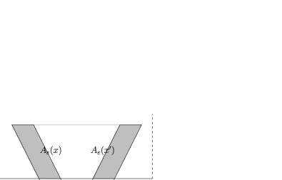
Figure 5: The error terms in the tree approximation correspond to the two grey parallelograms in Lemma .4.

References

- (1) {bbook}[mr] \bauthor\bsnmAdler, \bfnmRobert J.\binitsR. J. and \bauthor\bsnmTaylor, \bfnmJonathan E.\binitsJ. E. (\byear2007). \btitleRandom Fields and Geometry. \bpublisherSpringer, \blocationNew York. \bidmr=2319516 \bptokimsref\endbibitem
- (2) {barticle}[mr] \bauthor\bsnmArguin, \bfnmLouis-Pierre\binitsL.-P. and \bauthor\bsnmChatterjee, \bfnmSourav\binitsS. (\byear2013). \btitleRandom overlap structures: Properties and applications to spin glasses. \bjournalProbab. Theory Related Fields \bvolume156 \bpages375–413. \biddoi=10.1007/s00440-012-0431-6, issn=0178-8051, mr=3055263 \bptnotecheck year \bptokimsref\endbibitem
- (3) {barticle}[mr] \bauthor\bsnmBacry, \bfnmE.\binitsE. and \bauthor\bsnmMuzy, \bfnmJ. F.\binitsJ. F. (\byear2003). \btitleLog-infinitely divisible multifractal processes. \bjournalComm. Math. Phys. \bvolume236 \bpages449–475. \biddoi=10.1007/s00220-003-0827-3, issn=0010-3616, mr=2021198 \bptokimsref\endbibitem
- (4) {barticle}[mr] \bauthor\bsnmBarral, \bfnmJulien\binitsJ. and \bauthor\bsnmMandelbrot, \bfnmBenoît B.\binitsB. B. (\byear2002). \btitleMultifractal products of cylindrical pulses. \bjournalProbab. Theory Related Fields \bvolume124 \bpages409–430. \biddoi=10.1007/s004400200220, issn=0178-8051, mr=1939653 \bptokimsref\endbibitem
- (5) {barticle}[auto:STB—2013/12/09—07:59:19] \bauthor\bsnmBennett, \bfnmG.\binitsG. (\byear1962). \btitleProbability inequalities for the sum of independent random variables. \bjournalJ. Amer. Statist. Assoc. \bvolume57 \bpages33–45. \bptokimsref\endbibitem
- (6) {barticle}[mr] \bauthor\bsnmBolthausen, \bfnmErwin\binitsE., \bauthor\bsnmDeuschel, \bfnmJean-Dominique\binitsJ.-D. and \bauthor\bsnmGiacomin, \bfnmGiambattista\binitsG. (\byear2001). \btitleEntropic repulsion and the maximum of the two-dimensional harmonic crystal. \bjournalAnn. Probab. \bvolume29 \bpages1670–1692. \biddoi=10.1214/aop/1015345767, issn=0091-1798, mr=1880237 \bptokimsref\endbibitem
- (7) {barticle}[mr] \bauthor\bsnmBolthausen, \bfnmErwin\binitsE., \bauthor\bsnmDeuschel, \bfnmJean Dominique\binitsJ. D. and \bauthor\bsnmZeitouni, \bfnmOfer\binitsO. (\byear2011). \btitleRecursions and tightness for the maximum of the discrete, two dimensional Gaussian free field. \bjournalElectron. Commun. Probab. \bvolume16 \bpages114–119. \biddoi=10.1214/ECP.v16-1610, issn=1083-589X, mr=2772390 \bptokimsref\endbibitem
- (8) {barticle}[mr] \bauthor\bsnmBolthausen, \bfnmErwin\binitsE. and \bauthor\bsnmKistler, \bfnmNicola\binitsN. (\byear2006). \btitleOn a nonhierarchical version of the generalized random energy model. \bjournalAnn. Appl. Probab. \bvolume16 \bpages1–14. \biddoi=10.1214/105051605000000665, issn=1050-5164, mr=2209333 \bptokimsref\endbibitem
- (9) {barticle}[mr] \bauthor\bsnmBolthausen, \bfnmErwin\binitsE. and \bauthor\bsnmKistler, \bfnmNicola\binitsN. (\byear2009). \btitleOn a nonhierarchical version of the generalized random energy model. II. Ultrametricity. \bjournalStochastic Process. Appl. \bvolume119 \bpages2357–2386. \biddoi=10.1016/j.spa.2008.12.002, issn=0304-4149, mr=2531095 \bptokimsref\endbibitem
- (10) {bbook}[mr] \bauthor\bsnmBolthausen, \bfnmErwin\binitsE. and \bauthor\bsnmSznitman, \bfnmAlain-Sol\binitsA.-S. (\byear2002). \btitleTen Lectures on Random Media. \bseriesDMV Seminar \bvolume32. \bpublisherBirkhäuser, \blocationBasel. \biddoi=10.1007/978-3-0348-8159-3, mr=1890289 \bptokimsref\endbibitem
- (11) {barticle}[mr] \bauthor\bsnmBovier, \bfnmAnton\binitsA. and \bauthor\bsnmKurkova, \bfnmIrina\binitsI. (\byear2004). \btitleDerrida’s generalised random energy models. I. Models with finitely many hierarchies. \bjournalAnn. Inst. Henri Poincaré Probab. Stat. \bvolume40 \bpages439–480. \biddoi=10.1016/j.anihpb.2003.09.002, issn=0246-0203, mr=2070334 \bptokimsref\endbibitem
- (12) {barticle}[mr] \bauthor\bsnmBovier, \bfnmAnton\binitsA. and \bauthor\bsnmKurkova, \bfnmIrina\binitsI. (\byear2004). \btitleDerrida’s generalized random energy models. II. Models with continuous hierarchies. \bjournalAnn. Inst. Henri Poincaré Probab. Stat. \bvolume40 \bpages481–495. \biddoi=10.1016/j.anihpb.2003.09.003, issn=0246-0203, mr=2070335 \bptokimsref\endbibitem
- (13) {barticle}[mr] \bauthor\bsnmBramson, \bfnmMaury\binitsM. and \bauthor\bsnmZeitouni, \bfnmOfer\binitsO. (\byear2012). \btitleTightness of the recentered maximum of the two-dimensional discrete Gaussian free field. \bjournalComm. Pure Appl. Math. \bvolume65 \bpages1–20. \biddoi=10.1002/cpa.20390, issn=0010-3640, mr=2846636 \bptnotecheck year \bptokimsref\endbibitem
- (14) {barticle}[mr] \bauthor\bsnmCapocaccia, \bfnmD.\binitsD., \bauthor\bsnmCassandro, \bfnmM.\binitsM. and \bauthor\bsnmPicco, \bfnmP.\binitsP. (\byear1987). \btitleOn the existence of thermodynamics for the generalized random energy model. \bjournalJ. Stat. Phys. \bvolume46 \bpages493–505. \biddoi=10.1007/BF01013370, issn=0022-4715, mr=0883541 \bptokimsref\endbibitem
- (15) {barticle}[auto:STB—2013/12/09—07:59:19] \bauthor\bsnmCarpentier, \bfnmD.\binitsD. and \bauthor\bparticleLe \bsnmDoussal, \bfnmP.\binitsP. (\byear2001). \btitleGlass transition for a particle in a random potential, front selection in nonlinear renormalization group, and entropic phenomena in Liouville and Sinh-Gordon models. \bjournalPhys. Rev. E (3) \bvolume63 \bpages026110. \bptokimsref\endbibitem
- (16) {bincollection}[mr] \bauthor\bsnmChauvin, \bfnmB.\binitsB. and \bauthor\bsnmRouault, \bfnmA.\binitsA. (\byear1997). \btitleBoltzmann–Gibbs weights in the branching random walk. In \bbooktitleClassical and Modern Branching Processes (Minneapolis, MN, 1994) (\beditor\binitsK. B.\bfnmK. B. \bsnmAthreya and \beditor\binitsP.\bfnmP. \bsnmJagers, eds.). \bseriesIMA Vol. Math. Appl. \bvolume84 \bpages41–50. \bpublisherSpringer, \blocationNew York. \biddoi=10.1007/978-1-4612-1862-3_3, mr=1601693 \bptnotecheck year \bptokimsref\endbibitem
- (17) {barticle}[mr] \bauthor\bsnmDaviaud, \bfnmOlivier\binitsO. (\byear2006). \btitleExtremes of the discrete two-dimensional Gaussian free field. \bjournalAnn. Probab. \bvolume34 \bpages962–986. \biddoi=10.1214/009117906000000061, issn=0091-1798, mr=2243875 \bptokimsref\endbibitem
- (18) {barticle}[auto:STB—2013/12/09—07:59:19] \bauthor\bsnmDerrida, \bfnmB.\binitsB. (\byear1985). \btitleA generalisation of the random energy model that includes correlations between the energies. \bjournalJ. Phys. Lett. \bvolume46 \bpages401–407. \bptokimsref\endbibitem
- (19) {barticle}[mr] \bauthor\bsnmDerrida, \bfnmB.\binitsB. and \bauthor\bsnmSpohn, \bfnmH.\binitsH. (\byear1988). \btitlePolymers on disordered trees, spin glasses, and traveling waves. \bjournalJ. Stat. Phys. \bvolume51 \bpages817–840. \biddoi=10.1007/BF01014886, issn=0022-4715, mr=0971033 \bptokimsref\endbibitem
- (20) {barticle}[mr] \bauthor\bsnmDing, \bfnmJian\binitsJ. (\byear2013). \btitleExponential and double exponential tails for maximum of two-dimensional discrete Gaussian free field. \bjournalProbab. Theory Related Fields \bvolume157 \bpages285–299. \biddoi=10.1007/s00440-012-0457-9, issn=0178-8051, mr=3101848 \bptnotecheck year \bptokimsref\endbibitem
- (21) {barticle}[mr] \bauthor\bsnmDovbysh, \bfnmL. N.\binitsL. N. and \bauthor\bsnmSudakov, \bfnmV. N.\binitsV. N. (\byear1982). \btitleGram–de Finetti matrices. \bjournalJ. Soviet. Math. \bvolume24 \bpages3047–3054. \bptokimsref\endbibitem
- (22) {bbook}[mr] \bauthor\bsnmDurrett, \bfnmRichard\binitsR. (\byear2004). \btitleProbability: Theory and Examples, \bedition3rd ed. \bpublisherDuxbury Press, \blocationBelmont, CA. \bptokimsref\endbibitem
- (23) {barticle}[mr] \bauthor\bsnmFang, \bfnmMing\binitsM. and \bauthor\bsnmZeitouni, \bfnmOfer\binitsO. (\byear2012). \btitleBranching random walks in time inhomogeneous environments. \bjournalElectron. J. Probab. \bvolume17 \bpages1–18. \biddoi=10.1214/EJP.v17-2253, issn=1083-6489, mr=2968674 \bptokimsref\endbibitem
- (24) {barticle}[mr] \bauthor\bsnmFyodorov, \bfnmYan V.\binitsY. V. and \bauthor\bsnmBouchaud, \bfnmJean-Philippe\binitsJ.-P. (\byear2008). \btitleFreezing and extreme-value statistics in a random energy model with logarithmically correlated potential. \bjournalJ. Phys. A \bvolume41 \bpages372001, 12. \biddoi=10.1088/1751-8113/41/37/372001, issn=1751-8113, mr=2430565 \bptokimsref\endbibitem
- (25) {bmisc}[auto:STB—2013/12/09—07:59:19] \bauthor\bsnmFyodorov, \bfnmY. V.\binitsY. V., \bauthor\bparticleLe \bsnmDoussal, \bfnmP.\binitsP. and \bauthor\bsnmRosso, \bfnmA.\binitsA. (\byear2009). \bhowpublishedStatistical mechanics of logarithmic REM: Duality, freezing and extreme value statistics of noises generated by Gaussian free fields. J. Stat. Mech. 2009 P10005. \bptokimsref\endbibitem
- (26) {barticle}[mr] \bauthor\bsnmGhirlanda, \bfnmStefano\binitsS. and \bauthor\bsnmGuerra, \bfnmFrancesco\binitsF. (\byear1998). \btitleGeneral properties of overlap probability distributions in disordered spin systems. Towards Parisi ultrametricity. \bjournalJ. Phys. A \bvolume31 \bpages9149–9155. \biddoi=10.1088/0305-4470/31/46/006, issn=0305-4470, mr=1662161 \bptokimsref\endbibitem
- (27) {bbook}[mr] \bauthor\bsnmLedoux, \bfnmMichel\binitsM. and \bauthor\bsnmTalagrand, \bfnmMichel\binitsM. (\byear1991). \btitleProbability in Banach Spaces: Isoperimetry and Processes. \bseriesErgebnisse der Mathematik und Ihrer Grenzgebiete (3) \bvolume23. \bpublisherSpringer, \blocationBerlin. \bidmr=1102015 \bptokimsref\endbibitem
- (28) {barticle}[mr] \bauthor\bsnmPanchenko, \bfnmDmitry\binitsD. (\byear2010). \btitleA connection between the Ghirlanda–Guerra identities and ultrametricity. \bjournalAnn. Probab. \bvolume38 \bpages327–347. \biddoi=10.1214/09-AOP484, issn=0091-1798, mr=2599202 \bptokimsref\endbibitem
- (29) {barticle}[mr] \bauthor\bsnmPanchenko, \bfnmDmitry\binitsD. (\byear2010). \btitleThe Ghirlanda–Guerra identities for mixed -spin model. \bjournalC. R. Math. Acad. Sci. Paris \bvolume348 \bpages189–192. \biddoi=10.1016/j.crma.2010.02.004, issn=1631-073X, mr=2600075 \bptokimsref\endbibitem
- (30) {barticle}[mr] \bauthor\bsnmRobert, \bfnmRaoul\binitsR. and \bauthor\bsnmVargas, \bfnmVincent\binitsV. (\byear2010). \btitleGaussian multiplicative chaos revisited. \bjournalAnn. Probab. \bvolume38 \bpages605–631. \biddoi=10.1214/09-AOP490, issn=0091-1798, mr=2642887 \bptokimsref\endbibitem
- (31) {barticle}[mr] \bauthor\bsnmRuelle, \bfnmDavid\binitsD. (\byear1987). \btitleA mathematical reformulation of Derrida’s REM and GREM. \bjournalComm. Math. Phys. \bvolume108 \bpages225–239. \bidissn=0010-3616, mr=0875300 \bptokimsref\endbibitem
- (32) {bbook}[mr] \bauthor\bsnmSimon, \bfnmBarry\binitsB. (\byear1993). \btitleThe Statistical Mechanics of Lattice Gases. Vol. I. \bpublisherPrinceton Univ. Press, \blocationPrinceton, NJ. \bidmr=1239893 \bptokimsref\endbibitem
- (33) {bbook}[mr] \bauthor\bsnmTalagrand, \bfnmMichel\binitsM. (\byear2003). \btitleSpin Glasses: A Challenge for Mathematicians: Cavity and Mean Field Models. \bseriesErgebnisse der Mathematik und Ihrer Grenzgebiete. 3. Folge. \bvolume46. \bpublisherSpringer, \blocationBerlin. \bidmr=1993891 \bptokimsref\endbibitem
- (34) {barticle}[mr] \bauthor\bsnmTalagrand, \bfnmMichel\binitsM. (\byear2010). \btitleConstruction of pure states in mean field models for spin glasses. \bjournalProbab. Theory Related Fields \bvolume148 \bpages601–643. \biddoi=10.1007/s00440-009-0242-6, issn=0178-8051, mr=2678900 \bptokimsref\endbibitem