The Astro-WISE approach to quality control for astronomical data

Abstract

We present a novel approach to quality control during the processing of astronomical data. Quality control in the Astro-WISE Information System is integral to all aspects of data handing and provides transparent access to quality estimators for all stages of data reduction from the raw image to the final catalog. The implementation of quality control mechanisms relies on the core features in this Astro-WISE Environment(AWE): an object-oriented framework, full data lineage, and both forward and backward chaining. Quality control information can be accessed via the command-line awe-prompt and the web-based Quality-WISE service. The quality control system is described and qualified using archive data from the 8-CCD Wide Field Imager (WFI) instrument (http://www.eso.org/lasilla/instruments/wfi/) on the 2.2-m MPG/ESO telescope at La Silla and (pre-)survey data from the 32-CCD OmegaCAM instrument (http://www.astro-wise.org/$\sim$omegacam/) on the VST telescope at Paranal.

1 Introduction

Quality control is typically one of the greatest challenges in the chain from raw sensor data to scientific papers. This includes not only limited observations for an individual scientist such as subsets of archival WFI data, but also bulk observations of large astronomical surveys, such as those taken with OmegaCAM on the VST (VLT Survey Telescope). In such surveys, the human and financial resources required often dictate that not only the large survey teams are spread over many institutes in many countries, but also the required data storage and the parallel computing resources. Such a situation requires an environment in which all non-manual qualifications are automated and the scientist can graphically inspect where needed. This is easily achieved by going back and forth through the data and metadata of the whole processing chain for large numbers of data products, and for only those data products where it is necessary. Such efficiency is clearly as beneficial to individual scientists as it is to large survey teams.

These requirements force survey teams beyond the era of science on a desktop and dictate a paradigm in which astronomers, calibration scientists, and computer scientists spread over geographically distant locations in many countries share their work and latest results in a single environment that allows the optimized processing, quality control, and archiving of large data sets. This means a federated system of humans, databases, computing resources, and data storage yielding an integrated information system (Valentijn et al., 2007). This integrated information system, Astro-WISE, is introduced and described in detail in Begeman et al. (2011). It is assumed that the reader is familiar with the fundamental concepts described in these papers as only the most relevant concepts will be dealt with here.

1.1 Traditional quality control

The quality control of astronomical data is a key to success in obtaining necessary data for scientific use cases. Quality control allows scientists to verify observations, to improve observational plans, to correct the regime of observations, to check the data processing and, finally, to distinguish between an artifact and a real event detected during the observations.

Present day observations, especially the vast amounts in the case of large astronomical surveys, require complicated processing systems involving a number of data processing levels and programming efforts from many scientists and programmers, usually distributed over a number of institutions. Tracing data quality through the processing chain given the involvement of many scientists and institutions becomes a non-trivial but crucial task.

There are many efforts invested in checking the quality of data delivered by an instrument, but this quality control remains at the observation/reduction site and comes to the scientific user as a reduced set of parameters describing the quality of the observations (Hummel et al., 2010; Dobrzycka et al., 2008). There is no way for the user to return to the raw observational material and check the quality of a particular observation. In the case when the user does not process the data her/himself, but accesses only the final product, she/he has to rely on the model of the quality control chosen by the people behind the data processing. There is a general understanding that the quality control should be shared by the observers and scientists responsible for the data processing (Hanuschik, 2007). Nevertheless, this does not relieve the user from the task of making decision about the data quality based on incomplete and non-reproducible information provided with the end product.

One mechanism bulk data providers employ to describe the quality of data products is to introduce a number of attributes in the data model which will hold information related to the quality control. For example, in the case of 2MASS data products the quality control was performed during the observations and the data processing, and the final catalog was formed according to the algorithm described in Skrutskie et al. (2006). From 60 attributes of the Two Micron All Sky Survey Point Source Catalog (2MASS PSC), 31 attributes are related to data quality. This allows the user to create a subset according to his/her preferences for the quality of the data, but limits the user to the good quality data. The criteria for the data to be considered as good are defined for a survey, not for a user of its data. Similar approaches were used by SDSS and UKIDSS surveys. In all these cases, data are delivered in a catalog with uniform quality rather than optimizing quality for particular data subsets (Ivezić et al., 2004; Warren et al., 2007). This is contrary to the typical goal of an individual scientist using the final data products.

To make a sound decision about data quality, the user should be able to access quality control algorithms at any point from the observation to the creation of the end product. Thus, ideally, quality control should be performed on and reviewed at each processing step. As a result, the user can trace the origin of any problem associated with quality parameters back to the specific processing step and/or the data entity responsible for it.

1.2 Astro-WISE quality control

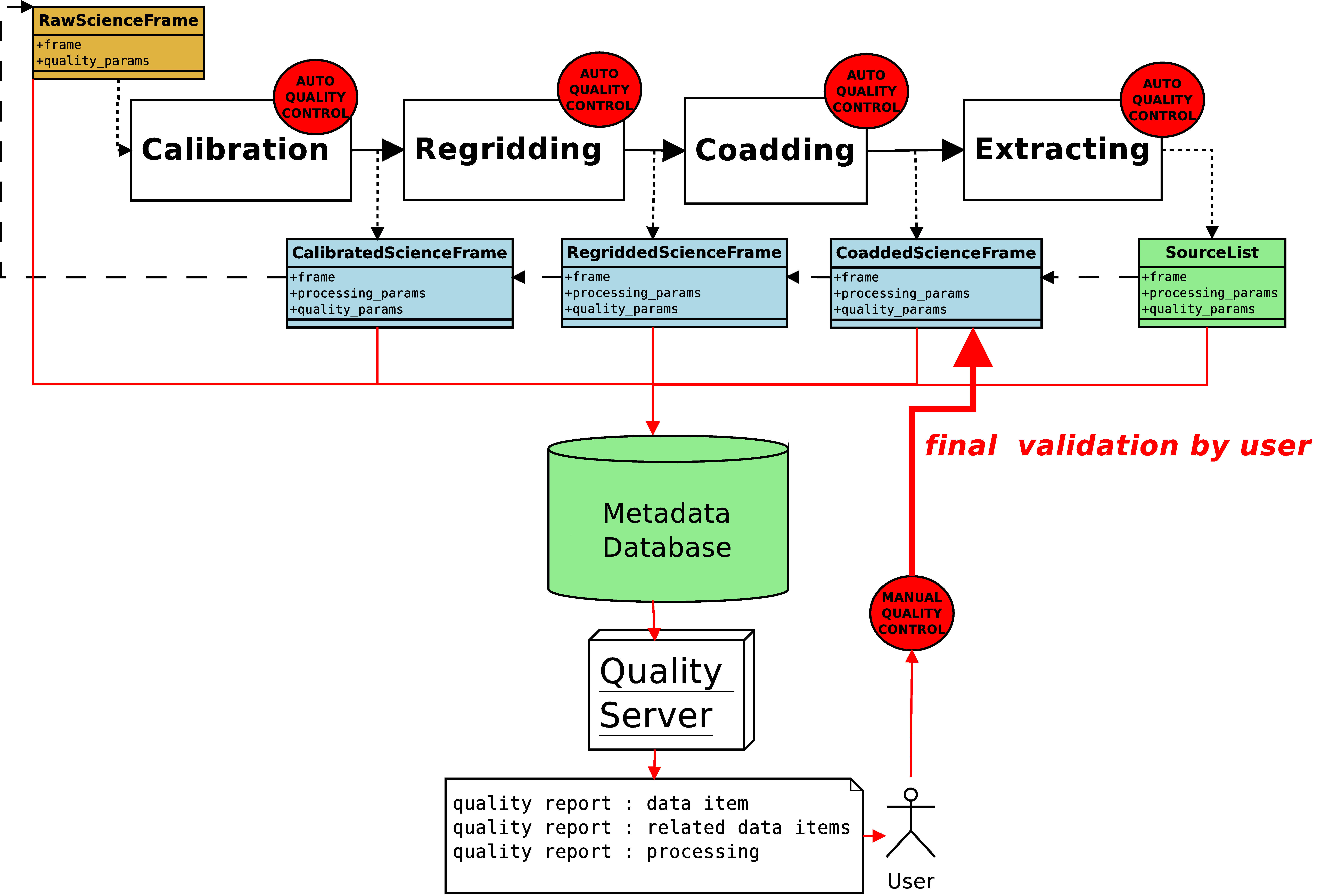
Figure 1: The quality control model in the Astro-WISE Information System. Shown is a schematic of the full data lineage with quality control at each processing step.

The core difference between this “traditional” quality control and the Astro-WISE approach to quality control is that the latter one uses features of Astro-WISE as an integrated information system to trace the quality at all stages of data production. These features are: data processing and quality control within the same system, an object-oriented framework, and full data lineage with both forward and backward chaining. Together, they allow testing of the quality of any data product, intermediate or final, from any other data product at any stage of processing or analysis. The advantages to this approach include allowing survey teams or individual scientists to inspect the quality of any data product, allowing reprocessing of all or only part of one or multiple data products in the most efficient way possible. In this way, the user knows exactly what the final quality means and can even reprocess any set of data to her/his needs.

Figure 1 shows an integral approach of quality control supported by the Astro-WISE Information System. There are two types of quality control at each stage of the data processing: automatic (default) and manual (optional). The user can visually inspect each data item and validate/invalidate it. All the information about the quality at every stage of data processing is saved in the database.

The object-oriented framework includes a set of parameters that are assigned to each data class, and forms a built-in system of general quality estimators. The following section describes these quality parameters used in the Astro-WISE Environment (AWE) and how they are connected between different types of data. Section 3 describes the quality control mechanisms built into AWE. Section 4 gives examples of how trends in any aspect of the data can be isolated using the command-line (awe-prompt). Finally, Section 5 describes the graphical interface for quality control in AWE.

2 Quality parameters

2.1 Data visibility

Visibility of data meeting the minimum level of quality to be processed in AWE is governed by privilege level and by validity (i.e., privileged data and data flagged as poor quality is hidden). Privileges in AWE are levels of accessibility for different groups, similar to permissions levels on a UNIX file system.

All data entities in AWE are instances of Object-Oriented Programming (OOP) objects. Validity, and thus the processability, is indicated by setting any or all of the following flag attributes of a given object:

1. is_valid – manual validity flag

2. quality_flags – automatic validity flag

3. timestamp_start/end – validity ranges in time (for calibrations only)

4. creation_date – the most recent valid data is the best

For instance, obviously poor quality data can be flagged by setting its is_valid attribute to 0, preventing it from ever being processed automatically. The calibrations used are determined by their timestamp_start, timestamp_end, and creation_date attributes (Which calibrations are valid for the given data?), and the quality of processed data by the automatic setting of its quality_flag attribute (Is the given data good enough?). Good quality data can then be flagged for promotion (is_valid $>1$) and eventually promoted in privilege by its creator (published from level 1 to 2) so it can be seen by the project manager who will decide if it is worthy to be promoted once again (published from level 2 to 3 or higher) to be seen by the greater community. In the end, publishing of data and results can be done by the manual setting of a single flag attribute.

The example below shows how the user can invalidate a particular bias frame for a particular instrument, detector and date using AWE.

awe> bias = BiasFrame.select(instrument=’WFI’, chip=’ccd57’,
....                         date=’2003-10-05’)
awe> print bias.is_valid
1
awe> context.update_is_valid(bias,0)
awe> print bias.is_valid
0

Note that the query returns the most recent, valid master bias object for the given criteria. This same mechanism is used to query for objects during processing.

2.2 Provenance: full dependency linking and data lineage

The Astro-WISE Environment uses its federated database (Begeman et al., 2011; Valentijn et al., 2007) to link all data products to their progenitors (dependencies), creating a full data lineage of the entire processing chain. This allows quick and simple troubleshooting of data results by looking at processing settings, calibrations and more. It also allows for direct monitoring of the progress of survey or individual observations, thus simplifying observation management. This data lineage also provides the ability to analyze trends in dependencies to aid in troubleshooting (see Sect. 4.1).

Raw data is linked to the final data product via database links within the data object, allowing all information about any piece of data to be accessed instantly. See Mwbaze et al. (2009) for a detailed description of AWE’s data lineage implementation. This data linking uses the power of OOP to create this framework in a natural and transparent way.

3 Built-in quality control mechanisms

In the Astro-WISE Environment, quality control permeates all aspects of the data reduction process. From the moment data enters the system, through all processing steps, to the final data product, data quality is retained and can be accessed transparently. This is accomplished by integrating quality control concepts at the lowest levels of the system.

3.1 Integrated quality control

Quality control of the reduction process in AWE is integrated directly into the objects. Three methods exist on all ProcessTargets (the afore mentioned OOP objects that describe data entities undergoing some level of processing):

• verify() compares values derived from the current ProcessTarget instance to known acceptable limits (e.g., image statistics) and automatically raises quality_flags if the limits are exceeded

• compare() compares values derived from the current ProcessTarget instance to those of the previous version and automatically raises quality_flags if the values are worse

• inspect() provides an interface for manual inspection of the current ProcessTarget instance (e.g., viewing the image pixels)

The quality control parameters are stored in two persistent properties of the object, is_valid and quality_flags. As mentioned before, the is_valid property is the manual flag used to validate or invalidate any ProcessTarget, and the quality_flags property stores the results of the automatic verification routines. This model shares similarities with other quality control “scoring” models (e.g., Hanuschik et al. (2008)) and is discussed in the processing context in Sect. 3.3.

To give examples in contrast to this model, the Sloan survey uses automated pipelines (e.g., runQA and matchQA) run separately from the processing pipeline to assess and report the quality of the data (Ivezić et al., 2004), and the UKIDSS survey employs the metadata storage of FITS images to convey quality parameters to the QC procedures (Warren et al. (2007) and reference D06 therein). The integrated nature of the quality parameters and procedures in AWE has clear advantages over these other models because the quality parameters are directly part of the ProcessTarget.

This integrated quality control is one of the simplest, yet most powerful aspects of AWE for survey operator and individual scientist alike. Both high and low quality data can be accessed via a simple query and the cause of the low quality can be known directly via the bit-masked value of its quality_flags attribute. Also, the nature of the queries in the processing recipes guarantees that low quality data is never processed unless it is manually specified.

This paradigm for quality control allows for construction of tools such as Quality-WISE that can act as the QC front-end of the entire system. Data quality (of both pixel data and its metadata) can be viewed through a simple interface. This interface allows access to flagging of data (triggering automatic reprocessing), to direct reprocessing of data and even to the quality of linked objects. This all exists within the information system allowing effective sharing of human resources.

Class	process_param	value	units
RawBiasFrame	max_bias_stdev	100.0	ADU
	max_bias_level	500.0	ADU
	max_bias_flatness	10.0	ADU
RawDomeFlatFrame	min_flat_mean	5000	ADU
	max_flat_mean	55000	ADU
RawTwilightFlatFrame	min_flat_mean	5000	ADU
	max_flat_mean	55000	ADU
ReadNoise	maximum_readnoise	5.0	ADU
	maximum_bias_difference	1.0	ADU
	maximum_readnoise_difference	0.5	ADU
GainLinearity	maximum_gain_difference	0.1	$e^{-}/$ADU
	minimum_gain	2.0	$e^{-}/$ADU
	maximum_gain	5.0	$e^{-}/$ADU
BiasFrame	maximum_stdev	10.0	ADU
	maximum_stdev_differ	10.0	ADU
	maximum_subwin_flatn	100000.0	ADU
	maximum_subwin_stdev	100000.0	ADU
HotPixelMap	maximum_hotpixelcount	50000
	maximum_hotpixelcount_difference	100
ColdPixelMap	maximum_coldpixelcount	80000
	maximum_coldpixelcount_difference	100
DomeFlatFrame	maximum_subwin_flatness	1000.0	ADU
	maximum_subwin_diff	1000.0	ADU
TwilightFlatFrame	maximum_subwin_flatness	1000.0	ADU
	maximum_subwin_diff	1000.0	ADU
	maximum_number_of_outliers	10000	ADU
MasterFlatFrame	maximum_subwin_diff	1000.0	ADU
PhotometricParameters	max_error	0.03	mag
AstrometricParameters	min_nref	15
	max_nref	1200
	max_sigma	1.0	arcsec
	max_rms	1.0	arcsec
	min_n_overlap	20
	max_n_overlap	20000
	max_sigma_overlap	0.1	arcsec
	max_rms_overlap	0.1	arcsec

Table 1: Representative examples of QC limits used by the automated verify() and compare() methods on the given class instances (objects). These examples are limited to calibration data and are derived from the requirements for the OmegaCAM instrument and updated based on experience with archive data of the WFI instrument. See the document page linked from the class name of appropriate links on http://doc.astro-wise.org/astro.main.html for more details.

3.2 Quality control during ingestion

A number of automatic, simple quality control procedures are executed at the lowest level of data interaction–ingestion into the system. These procedures are used to flag poor-quality data so they are excluded from further use. The procedures include checks on the median and standard deviation of the pixel values in bias exposures, and the exposure level of flat-fields. The levels at which flags are raised are instrument and detector chip dependent, as needed.

3.3 Quality control during processing

Quality control at the processing stage starts well before any actual processing is done. The selection of data to be processed is subject to the visibility mechanism (see Sect. 2.1). All processing tasks first check the validity and quality of candidate science data, and the validity, quality and timestamp ranges of applicable calibration data. This guarantees that only the highest quality data is considered for processing.

Once data processing is complete, the quality methods of data product object are run to verify that this is the highest quality product possible (see Sect. 3.1). The verify() and compare() methods are automatically run to check the data product against the accepted limits and to make sure the quality is higher than the previous version if one exists. If either test fails, one or more quality_flags are raised. Table 1 gives a representative sample of the limits tested via the verify() and compare() methods. Optionally, the inspect() method can be run manually to interactively check the data product. A non-interactive version of this method is always run to create and store a static version of the inspection plot for later perusal via the command-line or through the Quality-WISE service (see Sect. 5).

3.4 Inspection plots

During processing, quality control inspection plots are made as a matter of course. These can be viewed interactively during processing or saved for later viewing. As most processing is done in a parallel environment, these inspection plots tend to have a very low creation cost.

Inspection plots exist for many of the object types in AWE, particularly those critical for assessing the quality of major data products (e.g., science data quality, end-to-end detrending quality, astrometric and photometric calibration quality). See Fig. 2 through 6 for examples of such plots.

These static plots are simple snapshots of the most useful information to be inspected. In AWE, there exists the ability in most cases to interact with the inspection plot. This is done using the PyLab interface to MatPlotLib. This interface is integrated into AWE, and forms the backbone of all types of plotting, including post-processing analysis.

Figure 2: (left panel) A thumbnail representation of a WFI ReducedScienceFrame created by STIFF. The optimized intensity cuts and binning allow a quick assessment of the quality. This particular example shows an intensity gradient caused by either poor flat fielding, nebulosity from a galaxy at the center of the mosaic field (to the upper left), or simply a non-uniform illumination of the focal plane. The intensity values are inverted. (right panel) A thumbnail representation of a WFI WeightFrame created by STIFF. The optimized intensity cuts and binning allow a quick assessment of the quality. This particular example is associated with the thumbnail in the left panel. Saturated stellar peaks and bad columns are clearly visible in addition to “doughnuts” of the primary mirror of the telescope that are part of the flat field foundation of the WeightFrame. White pixels have values near 1, black pixels have values at or near 0. The horizontal lines are artifacts of the CCD manufacturing process. The higher weight of the pixels near some of the bad columns is an artifact caused by Fourier processing of input flat frames without properly taking into account bad pixels. It is possible to identify some of these defects with pixel statistics a priori, but these unusual cases are generally only identified through this type of inspection plot.

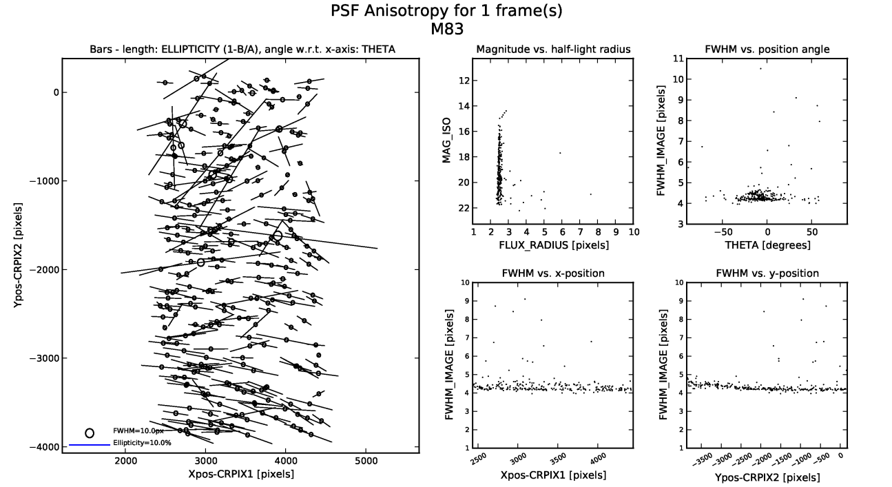
Figure 3: A PSF Anisotropy plot of the ReducedScienceFrame whose thumbnail is seen in Fig. 2. The left panel shows the two-dimensional anisotropy in the PSF (in both FWHM and in ellipticity) of the sources. The top-middle panel shows source magnitudes on an arbitrary scale versus flux radius and gives an indication of how “stellar” the sample is. The remaining panels plot FWHM of the sources versus ellipticity position angle, horizontal position and vertical position, respectively, clockwise from top-right.

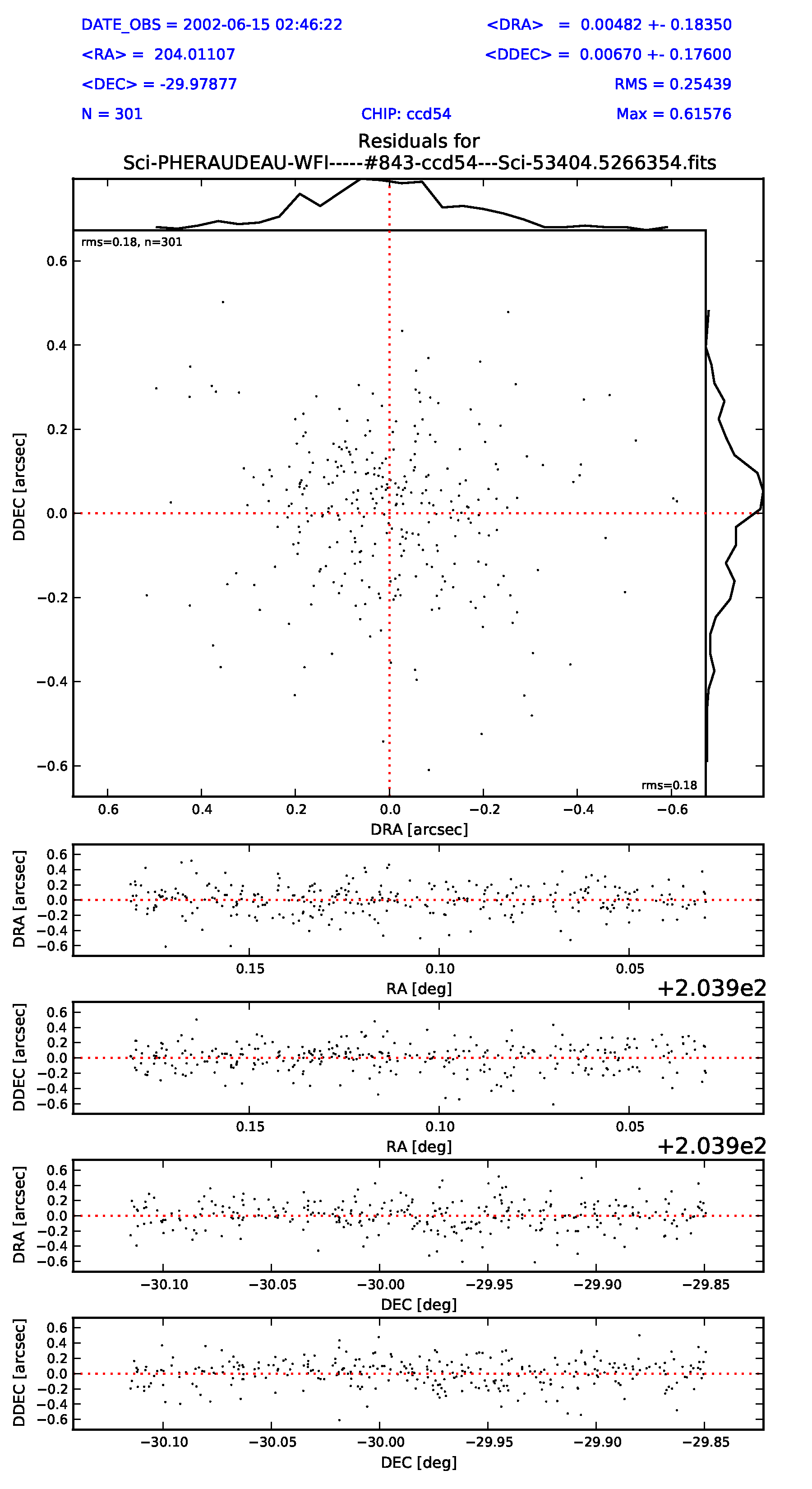
Figure 4: An AstrometricParameters inspection plot for a recent solution of the ReducedScienceFrame associated with the thumbnail in Fig. 2. The plot displays the statistics of the residuals (DRA and DDEC) between the RA and DEC of sources in a source catalog to which the local astrometric solution has been applied and the RA and DEC of those sources as listed in the reference catalog of astrometric standards, USNO-A2.0 in this case. The text in the top of the figure lists the observation date (DATE_OBS), the number (N) of sources pairs plotted, their average RA ($<$RA$>$) and DEC ($<$DEC$>$) in degrees, the average RA and DEC residuals ($<$DRA$>$ and $<$DDEC$>$) and their standard deviations in arcsec, and finally the root-mean-square (RMS) of the two-dimensional residual and the maximum two-dimensional residual (Max) in arcsec. The large upper panel plots DRA versus DDEC. The four panels below it show DRA and DDEC with respect to RA (with a constant offset of 203.9 degrees) and then to DEC.

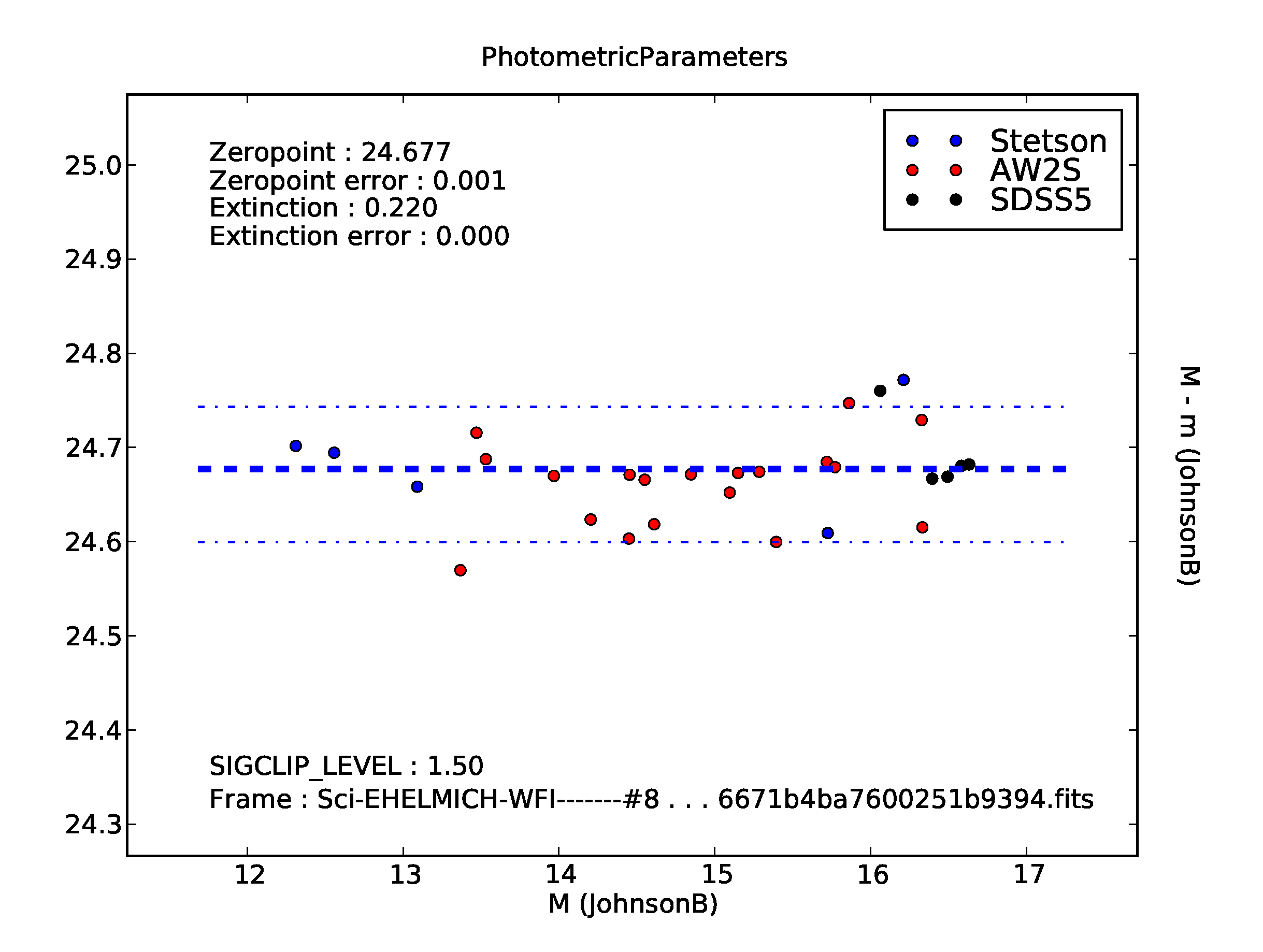
Figure 5: A PhotometricParameters inspection plot for a photometric observation comprising one WFI detector. A graphical representation of the data used to calculate the photometric zeropoint. In this plot, three photometric reference catalogs can be seen: Stetson (blue points), Astro-WISE secondary standards (red points) and Sloan Digital Sky Survey data release 5 (black points).

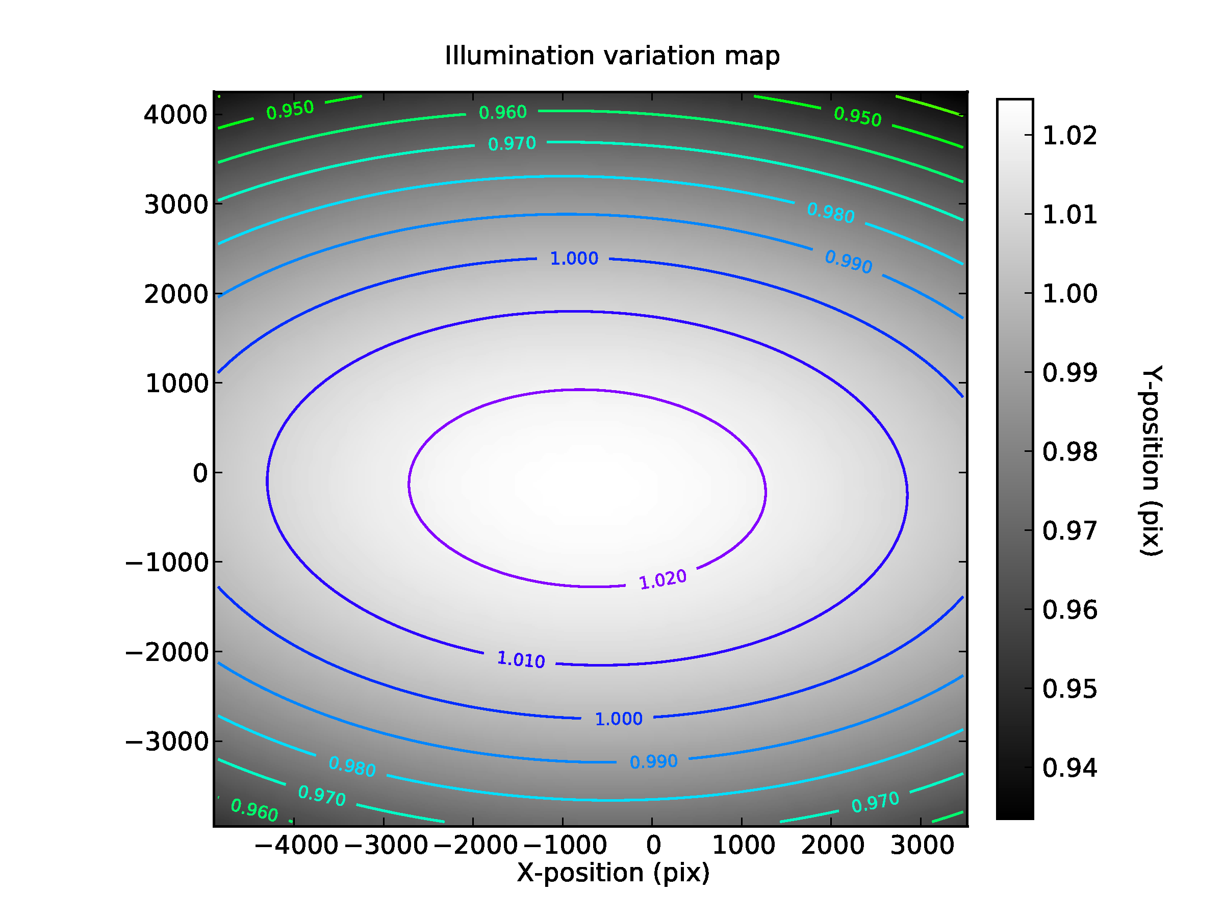
Figure 6: An IlluminationCorrection inspection plot for WFI data. This plot is a schematic representation of the illumination variations across the region of consideration, usually the entire field-of-view, eight 2k$\times$4k detectors in this case.

4 Trend analysis

Many powerful ways exist in the Astro-WISE Environment to examine both pixel data and metadata. One of these ways is through the use of the command-line interface, the awe-prompt. Through this interface, one can examine individual quality parameters and processing parameters of any object or linked object transparently.

4.1 Five-line script

AWE consists of Python classes representing ProcessTargets that can be created by scripts (called recipes or Tasks). The Tasks are simply sophisticated versions of what are termed five-line scripts (5LS). It is these 5LSs that do the bulk of the work of the data reduction and analysis for the user. The 5LS is also a powerful tool for quality control as atypical objects can be isolated easily.

This 5LS concept is a very simple and powerful way for users to interact with the data contained in the system. They can be “one-off”, “on-the-fly”, or “throw-away” scripts used to locate some interesting aspect of the data, can be written down in a source file for potential use at a later time, or can be integrated into an existing or future Task for the benefit of the system. One set of examples of 5LSs focuses on seeing how aspects of raw data in the system change over time, another gathers statistical data for comparison and outlier detection, and the last quickly investigates a scientific aspect of existing data in the system.

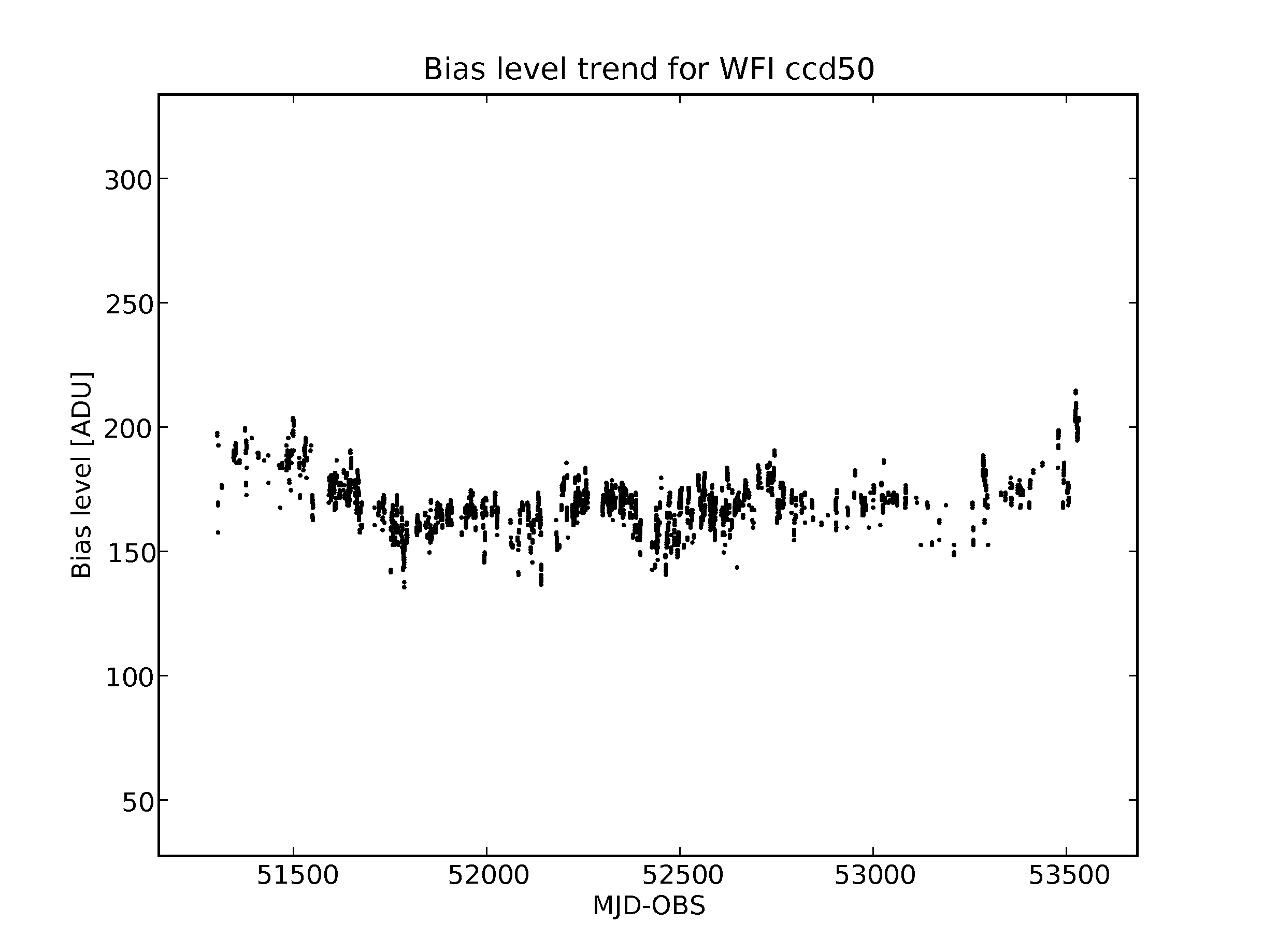
Figure 7: Plot of the bias level (median value of the science region) of ccd50 of the WFI instrument from May 1999 to June 2005.

4.2 Bias levels

Display the bias level as a function of time for chip ccd50 of the WFI camera:

awe> q = (RawBiasFrame.chip.name == ’ccd50’) &\
....     (RawBiasFrame.quality_flags == 0) &\
....     (RawBiasFrame.is_valid > 0)
....
awe> biases = list(q)  # instantiate all biases
awe> x = [b.MJD_OBS for b in biases]
awe> y = [b.imstat.median for b in biases]
awe> pylab.scatter(x,y,s=0.5)

This script will result in a plot similar to that seen in Fig. 7. It is important to note how the query is done. Not only are the objects of the desired detector queried for, the quality and validity (see Sect. 2.1) are also checked. This prevents any data that are out of specified ranges from being plotted, thus removing the worst outliers in the resulting plot before the data is even compiled. This lends significant efficiency to this method of visualization.

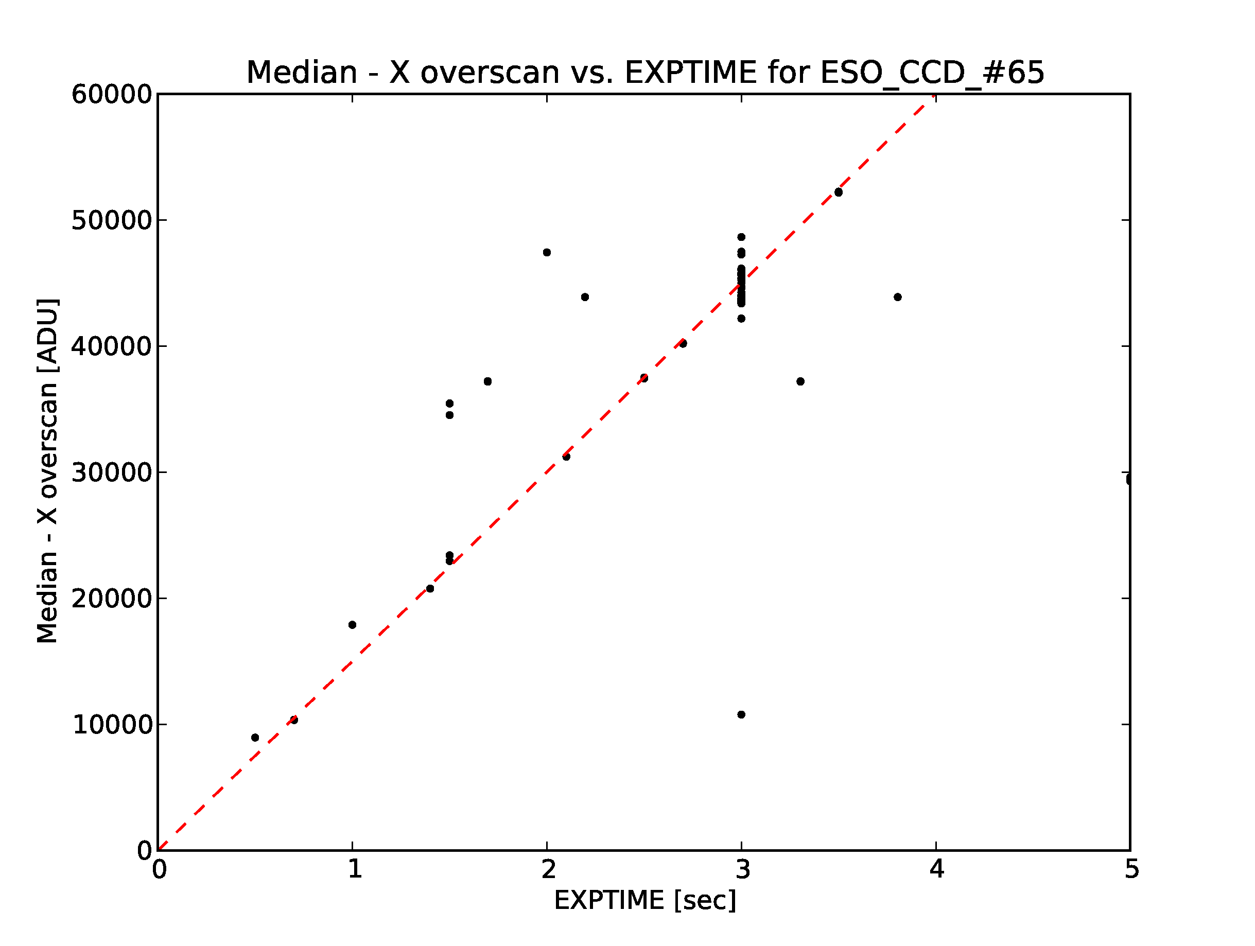
Figure 8: Plot of the dome flat exposure level (median value of the science region minus the median value of the X overscan region) versus exposure time of ESO_CCD_#65 of the OmegaCAM instrument from data taken in 2011. This plot gives a quick indication of how linear this detector is. The dashed red line is only an indication of the slope in the data. The cluster of points at EXPTIME$=$3 sec is from heavier sampling for diagnostic and detector health purposes.

4.3 Exposure levels

Not only can simple values be plotted over time as in the previous section, but more complex investigations of object attributes can be performed easily. In this set of examples, the linearity of an OmegaCAM detector is investigated:

awe> q = list((RawDomeFlatFrame.chip.name == ’ESO_CCD_#65’) &
....          (RawDomeFlatFrame.filter.name == ’OCAM_g_SDSS’) &
....          (RawDomeFlatFrame.quality_flags == 0) &
....          (RawDomeFlatFrame.is_valid > 0))
....
awe> exptime = [d.EXPTIME for d in q]
awe> med = [d.imstat.median-d.overscan_x_stat.median for d in q]
awe> pylab.plot(exptime, med, ’k.’)
awe> pylab.plot([0,4], [0,60000], ’r--’)

This first example gives a plot similar to that shown in Fig. 8. It is the overscan-corrected counts compared to the exposure time for one detector of the OmegaCAM mosaic. Simple arithmetic is seen in the list comprehension that creates the med list. The second example uses the data from the first, but adds the ability to perform array arithmetic using NumPy to plot the desired result (Fig. 9).

awe> med = numpy.array(med)
awe> exptime = numpy.array(exptime)
awe> pylab.plot(med, med/exptime, ’k.’)
awe> pylab.plot([0,60000], [15000,15000], ’r--’)

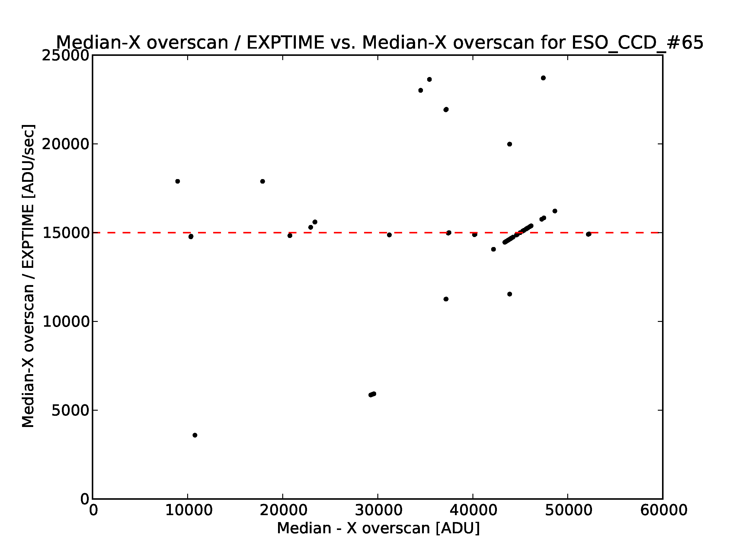
Figure 9: Plot of the dome flat exposure (median value of the science region minus the median value of the X overscan region divided by the exposure time) versus the dome flat exposure level (median value of the science region minus the median value of the X overscan region) of ESO_CCD_#65 of the OmegaCAM instrument from data taken in 2011. This plot quickly gives a different view of how linear this detector is. The dashed red line is only an indication of the mean detector exposure.

This second example gives a quick exposure time-independent view of the same data. As in the result of the previous script, outliers can easily be seen. It is now easy to isolate these outliers with NumPy methods using visually chosen limits:

awe> outlier_mask  = (med/exptime < 10000)
awe> outlier_mask |= (med/exptime > 20000)
awe> outliers = med[outlier_mask], exptime[outlier_mask]
awe> good_data = med[~outlier_mask], exptime[~outlier_mask]

4.4 Twenty thousand light curves

In the Fall of 2006, an investigation of light curves of the stars in the region of Centaurus-A was undertaken using pre-reduced data in the Astro-WISE system. The data was originally observed in the first half of 2005 with the WFI instrument. Only example scripts and resulting plots are reproduced here. The scripts have been updated and reformatted for inclusion.

The first example takes data from an association of two coadded frames. These data exist in the system as an AssociateList object. Some astrometric and photometric parameters are mined from the association data. This is plotted in such a way to test the astrometric accuracy of fainter sources (see Fig. 10). The plot clearly shows a slight degradation in this accuracy, but also shows that it is not a source of concern as the position of faintest sources is still generally well known.

awe> Al = (AssociateList.ALID == 1431)[0]
awe> arlist =  [’RA’, ’DEC’, ’MAG_ISO’, ’MAG_AUTO’, ’MAG_APER’]
awe> r = Al.get_data_on_associates(arlist,mask=3,mode=’ALL’)
awe> mag, dmag, ddec = [], [], []
awe> for aid in r.keys():
....     # index 0 = SLID, 1 = SID, # added automatically
....     # index 3 = DEC, 5 = MAG_AUTO
....     mag.append(r[aid][0][5])
....     dmag.append(r[aid][0][5] - r[aid][1][5])
....     ddec.append((r[aid][0][3] - r[aid][1][3])*3600)
....
awe> pylab.plot(mag, dmag, ’b.’, ms=0.5)
awe> pylab.plot(mag, ddec, ’r.’, ms=0.2)
awe> pylab.ylim([-2,2])

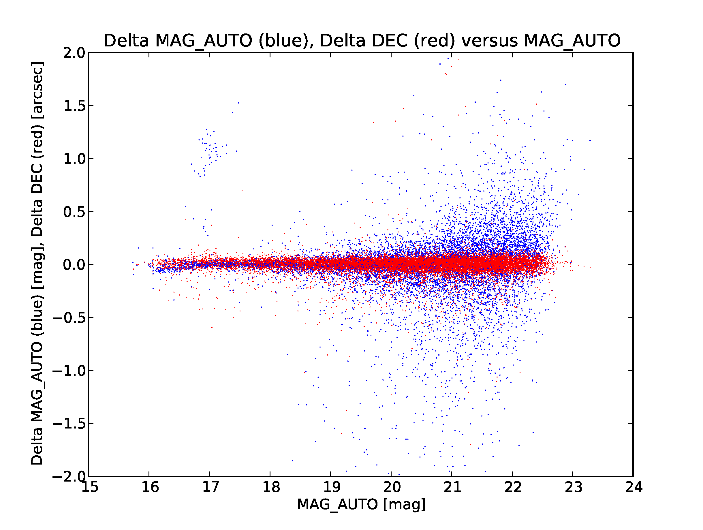
Figure 10: A plot of delta MAG_AUTO (blue points) over-plotted with delta DEC (red points) versus MAG_AUTO. The increase in scatter of the astrometric residuals is far lower than that of the photometric residual, a qualitative indication that astrometry for faint sources is at acceptable levels.

The next example mines data and creates a plot of light curves for approximately 7500 of the 20000 stars associated with at least one other star in one of the other observations. These 7500 are the stars that were associated for all 12 observations (i.e., where photometric data exists for all 12 observations). For brevity and clarity, only the first 100 of these are plotted by the script and shown in the accompanying plot (see Fig. 11).

awe> Al = (AssociateList.ALID == 1534)[0]
awe> sls = Al.sourcelists
awe> dates = [sl.frame.observing_block.start for sl in sls]
awe> arlist =  [’RA’, ’DEC’, ’MAG_ISO’, ’MAG_AUTO’, ’MAG_APER’]
awe> r = Al.get_data_on_associates(arlist, count=len(dates))
awe> #for aid in r.keys():      # plots eveything
awe> for aid in r.keys()[:100]: # plots only first 100 stars
....     # index 5 = MAG_AUTO
....     mags = [r[aid][i][5] for i in range(len(r[aid]))]
....     datesmags = zip(dates,mags) # sort by obsdate
....     datesmags.sort()
....     date = [datemag[0] for datemag in datesmags]
....     mag = [datemag[1] for datemag in datesmags]
....     l = pylab.plot(date, mag ,’k.’, date, mag, ’-’)
....
awe> dt1 = datetime.datetime(2005,3,1)
awe> dt2 = datetime.datetime(2005,6,15)
awe> pylab.xlim(dt1, dt2)

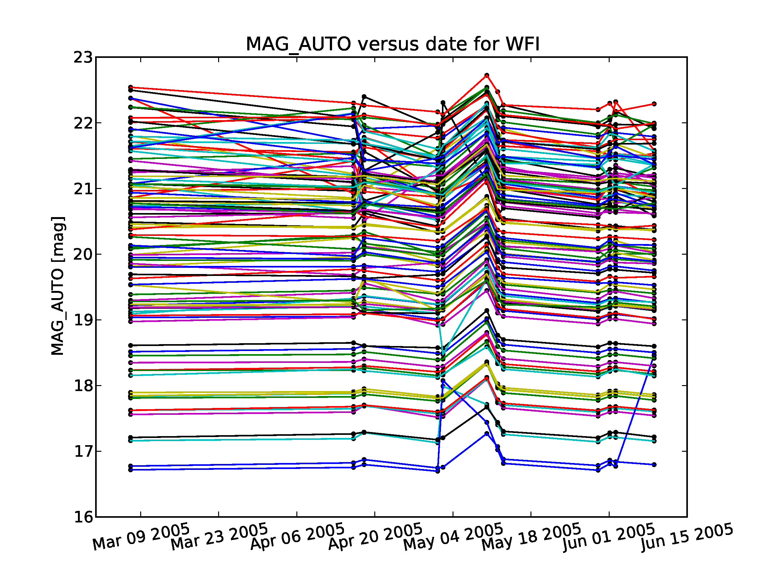
Figure 11: A plot of MAG_AUTO versus the date for 100 of approximately 7500 light-curves containing 12 photometric data points. It is obvious that there remain systematic offsets in the zeropoints.

In this last example, the zeropoint of each chip is compared over time with the zeropoints of all the other chips. The results can be seen in Fig. 12.

awe> for chip in context.get_chips_for_instrument(’WFI’):
....     zeropnts = []
....     for sl in sls:
....         for reg in sl.frame.regridded_frames:
....             if reg.chip.name == chip:
....                 red = reg.reduced
....                 break
....         pht = PhotometricParameters.select_for_reduced(red)
....         zeropnts.append(pht.zeropnt.value)
....     dateszps = zip(dates, zeropnts)
....     dateszps.sort()
....     date = [datezp[0] for datezp in dateszps]
....     zeropnt = [datezp[1] for datezp in dateszps]
....     pylab.plot(date, zeropnt, ’k.’, date, zeropnt, ’-’)
....
awe> pylab.xlim(dt1, dt2)

Zeropoint residuals with respect to that of any chip or to the mean zeropoint per day can easily be obtained with only slight additions to the example code presented above. This can give a clearer view of how the zeropoint of the set of chips evolves over time.

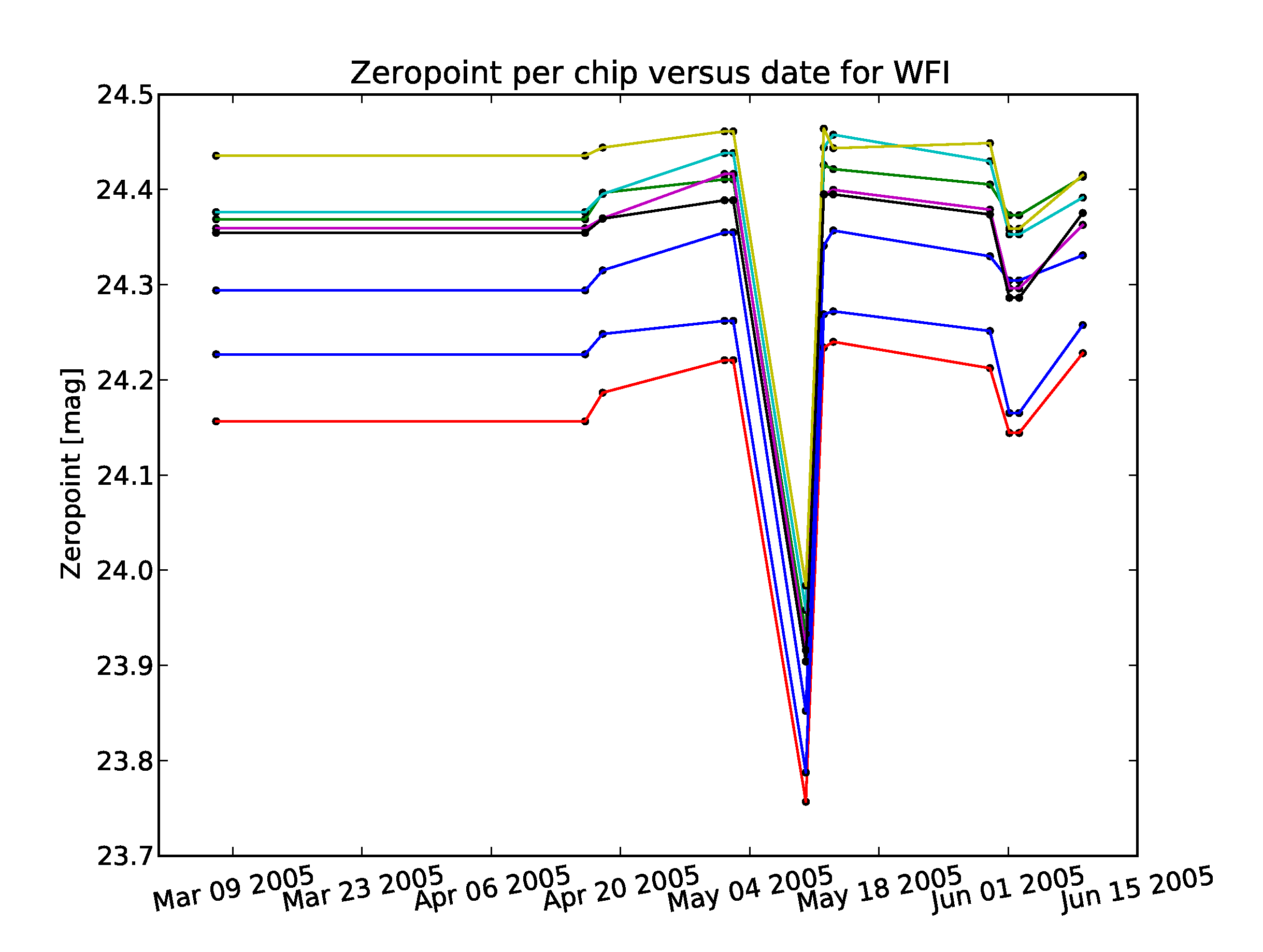
Figure 12: A plot of zeropoint versus the date for all 8 WFI detectors. The systematic offsets in zeropoint from night to night is clearly seen.

5 Quality-WISE web service

All objects stored in the Astro-WISE database are stored with their processing and quality parameters. These parameters can be accessed in many ways: from the command-line interface queries, from direct access to the database, or from web services such as CalTS (calts.astro-wise.org) or DBView (dbview.astro-wise.org). In Astro-WISE Environment, we have implemented a quality web service that combines all three methods and collects the most relevant metadata for the purpose of quality control: quality.astro-wise.org.

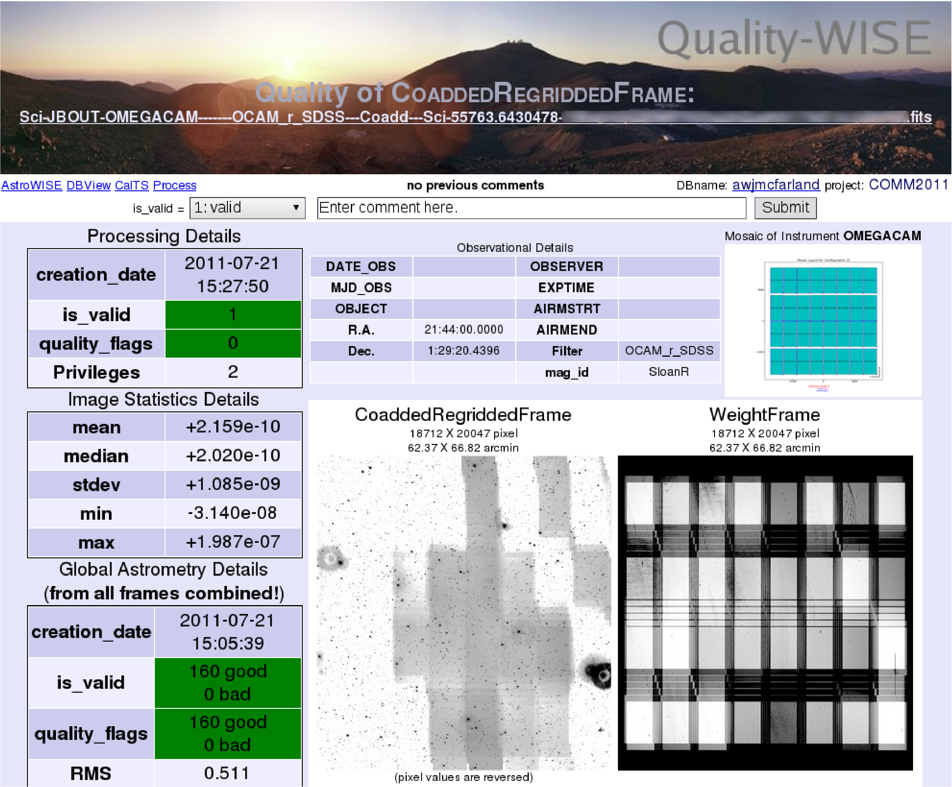
Figure 13: Screen-shot of the upper part of a Quality-WISE page. This view shows the quality of an OmegaCAM coadded frame. At the very top is the type of object and a link to the file on the dataserver (a unique hash value in the filename link is purposely obscured for security reasons). Directly below the banner is the top bar with links and basic actions. Below this is tabular information about the object and graphical inspection plots (a thumbnail of the image on the left and its weights on the right, cf. Fig. 2). Note that green fields indicate values within specified ranges that will be red when out of specified ranges.

The Quality-WISE interface is accessed primarily through the DBView service by clicking on the quality links associated with science data objects. The linked quality pages summarize observational and statistical details and add a schematic representation of the detector, thumbnails of pixel data, and various derived inspection plots (see Sect. 3.4). A basic interface is also included to flag or to publish data directly. Links to the quality pages of associated objects (e.g., progenitor or derived data products) also exist. Details of how the Quality-WISE service can be applied to real-world applications can be found in Verdoes et al. (2009).

5.1 Quality-WISE top bar

At the top of every Quality-WISE page is the class name of the object and a link to the associated data file on a data server (see Fig. 13). There is a bar below the banner image with links on the left to the Astro-WISE homepage and to the database viewer, calibration timestamps and target processor web services. On the right is the currently logged-in user and project name. These link to interfaces to change the user and/or the project via browser cookies. In the center, there is an indication of comments associated with the object and an interface to add comments. This is typically done when the validity of the object is changed using the is_valid interface. This interface allows one of 3 levels of validity to be assigned: $0=invalid$, $1=valid$ or $2=publishable$ (see Sect. 2.1). Pressing the Submit button stores the validity value and comment, where applicable, prior to reloading the quality page. For special purposes such as surveys, the validity choices can be expanded and the comment interface can have pre-specified strings included for efficiency.

5.2 Observational details

The observational details for the object being inspected are directly below the top bar of a Quality-WISE page (see Fig. 13). The values are taken directly from the object stored in the database and include: date of the observation in human readable and modified Julian date (DATE_OBS and MJD_OBS, respectively), the name of the object observed (OBJECT), right ascension and declination coordinates (R.A. and Dec., respectively), the observer responsible for the observation (OBSERVER), the exposure time (EXPTIME), the airmass at the start and end of the observation (AIRMSTRT and AIRMEND, respectively), the filter used for the observation (Filter), and the magnitude identifier of the filter, i.e., the photometric system (mag_id).

To the right of the observational details table is a graphical representation of the detector-plane layout for the individual detectors. The detectors highlighted in light blue are those that participated in the current data object. In the example of a CoaddedRegriddedFrame here, all detectors are highlighted as all detectors are represented in the data.

5.3 Processing and statistical details

On the left side of every Quality-WISE page are processing details and statistics of the main and associated objects (see Fig. 13). The main characteristic of this side bar is the highlighting of important quality parameters (see Table 1). When a parameter is within a specified range indicating good quality, the entire cell is colored green, when the parameter is outside this range, the entire cell is colored red. In addition, when the cursor is positioned over any of these cells, the reason for the indicated quality is displayed.

Processing details show when the object was created (creation_date), its validity (is_valid), if any quality flags have been set (quality_flags), and to what level it has been published (Privileges). See Sect. 2.1 for more on these last three parameters. Furthermore, statistics of the main object and associated astrometric and photometric objects, if any, are also listed (see also Fig. 14).

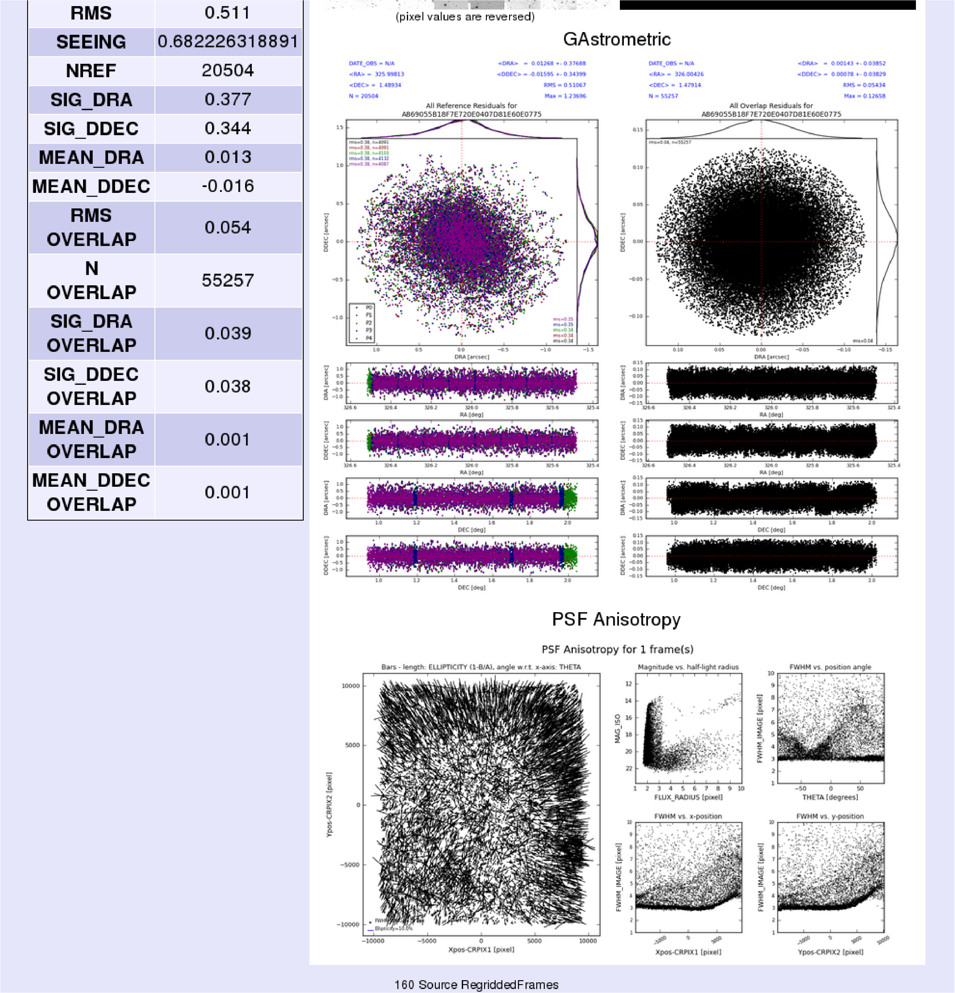
Figure 14: Screen-shot of the middle part of the Quality-WISE page shown in Fig. 13. The remainder of the statistical information of the combined global astrometric solution can be seen on the left. The astrometric residuals plots representing the quality of the solutions used to make the coadded frame are on the top-right. The PSF anisotropy plot for the coadded frame is at the bottom.

5.4 Inspection plots

The main body of each Quality-WISE page is dominated by the inspection plots. These plots are of the sort described in Sect. 3.4. They always start with an image thumbnail (with reverse pixel values) and a weight thumbnail (when applicable) showing lower weights as darker values (see Fig. 13). Below this is the astrometric reference residuals plot of the individual reduced frame local solution, or the astrometric reference and overlap residuals plots of the composite global solution for coadded frames (see Fig. 14). In this latter case, the additional plot shows the internal accuracy of the global solution. Below the astrometric plots can be the photometric plots showing the data used to derive the zero point and the results of the illumination correction derivation (see Figures 5 and 6). These are only shown for non-coadded objects. The last plot shown is the PSF anisotropy of the sources in the observation shown at the bottom of Fig. 14.

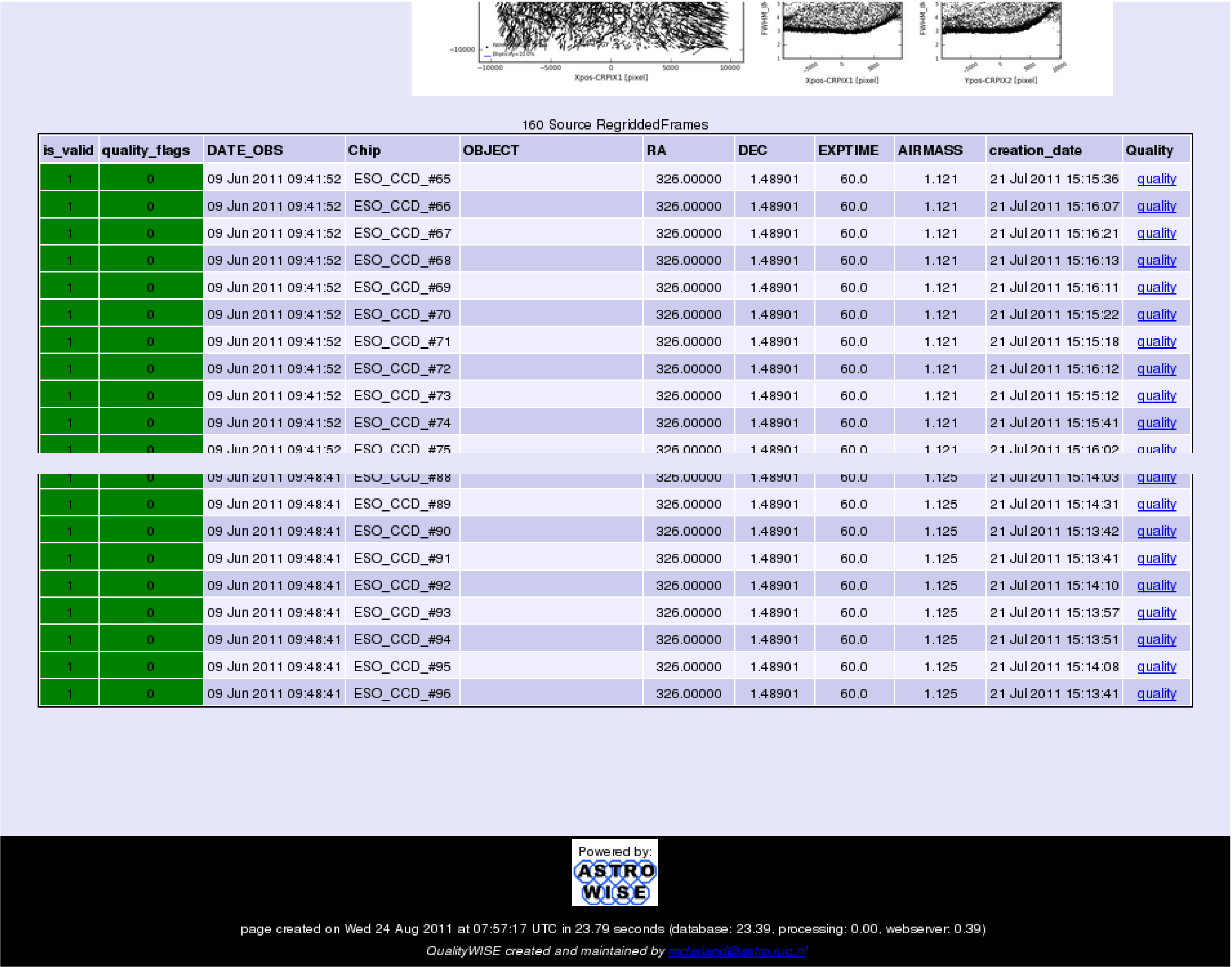
Figure 15: Screen-shot of the lower part of the Quality-WISE page shown in Figures 13 and 14. Near the top is the list of progenitor frames’ information. This list contains 160 entries and is truncated here. Basic information about the progenitor frames is provided in this list along with links to their quality pages (far right). Page creation information is presented at the very bottom including a breakdown of creation times into three bins: database time, processing time and web server time.

5.5 Progenitor/derived quality

For science data, each data product has progenitor data and derived data. The quality pages for these data are linked near the bottom. In the case of the CoaddedRegriddedFrame quality page in Fig. 15, there is only progenitor data. This consists of a list of 160 RegriddedFrames. The information listed is nearly identical to that described in the observational details table (see Sect. 5.2). At the far right of each entry is the link to the quality page of the progenitor object.

6 Summary

The approach for quality control of astronomical data in the Astro-WISE Information System has been described. The comparison to quality control techniques used in other systems has been presented. It was shown that the Astro-WISE approach has advantages for any individual user or group of users in that it allows the quality to be assessed for not only the final data product, but also any other progenitor data product in a simple and transparent way through database linking of all data objects (ProcessTargets).

This quality control is built into all aspects of the Astro-WISE information system. From the point where raw data enters the system, through all processing steps to the final data product, quality control mechanisms permeate throughout. Moreover, the quality of any stage of data processing can be assessed with quality parameters and inspection plots.

Using metadata (quality- or non-quality-related) stored in all linked objects, diagnostic plots can be created quickly using a relatively small amount of command-line code. This has been shown with examples using archive data from the WFI instrument at La Silla Observatory and (pre-)survey data from the newly commissioned OmegaCAM instrument at the Paranal Observatory. The code can be added to simple scripts for the benefit of the individual user, or eventually find its way into the core of the system benefiting all users alike.

All the quality control aspects of the Astro-WISE Environment have been gathered into a webservice called Quality-WISE. This service allows quick viewing of the metadata and inspection plots of the data in question and of any progenitor or derived data. It also provides a simple interface for a user or group of users to validate data and comment on its quality.

Taken as a whole, the Astro-WISE approach to quality control is a comprehensive and efficient method to perform quality checks on individual users’ data or on the data from large astronomical surveys. It is constantly being updated as newer, better quality control methods are discovered or derived, and will always stay on the cutting edge to maintain its advantages.