Low Complexity Turbo-Equalization: A Clustering Approach

Abstract

We introduce a low complexity approach to iterative equalization and decoding, or “turbo equalization”, that uses clustered models to better match the nonlinear relationship that exists between likelihood information from a channel decoder and the symbol estimates that arise in soft-input channel equalization. The introduced clustered turbo equalizer uses piecewise linear models to capture the nonlinear dependency of the linear minimum mean square error (MMSE) symbol estimate on the symbol likelihoods produced by the channel decoder and maintains a computational complexity that is only linear in the channel memory. By partitioning the space of likelihood information from the decoder, based on either hard or soft clustering, and using locally-linear adaptive equalizers within each clustered region, the performance gap between the linear MMSE equalizer and low-complexity, LMS-based linear turbo equalizers can be dramatically narrowed.

I Introduction

Digital communication receivers typically employ a symbol detector to estimate the transmitted channel symbols and a channel decoder to decode the error correcting code that was used to protect the information bits before transmission. There has been great interest in enabling interaction between the symbol estimation task and the channel decoding task, which is often termed “turbo equalization” for digital communication over channels with inter-symbol-interference (ISI). This interest is due to the dramatic performance gains that can be obtained with modest complexity[1] over performing these tasks separately. Turbo equalization methods employing maximum-a-posteriori probability (MAP) detectors demonstrate excellent bit-error-rate (BER) performance, however their computational complexity often renders their application impractical [1]. As an alternative, linear MMSE-based methods offer comparable performance to MAP-based approaches, with dramatically reduced complexity [1], compared with the exponential complexity of the MAP-based approach. However, MMSE-based approaches still require quadratic computational complexity in the channel length per output symbol and require adequate channel knowledge or estimation. To further reduce computational complexity and improve efficacy over unknown or time-varying channels, “direct” LMS-adaptive linear equalizers are often used, employing only linear complexity [2] in the regressor vector length, which is often on the order of the channel delay spread.

While these direct-adaptive methods may reduce computational complexity and can be shown to converge to their Wiener (MMSE) solution under stationary environments, they usually deliver inferior performance compared to linear MMSE-based methods. A primary reason for this performance loss is that the Wiener solution is not time-adaptive, but rather corresponds to the solution of the “stationarized problem” where the likelihood information from the decoder (which is by definition a sample-by-sample probability distribution over the transmitted data sequence and hence non-stationary) is replaced by a suitable time-averaged quantity [2]. On the other hand, both the linear MMSE and MAP-based turbo equalizer (TEQ) consider the log-likelihood ratio (LLR) sequence as time-varying a priori statistics over the transmitted symbols. This LLR information is used to construct the linear MMSE equalizer, which depends nonlinearly and in a time dependent manner on the LLR sequence.

In order to reduce the performance gap between LMS-adaptive linear TEQ and linear MMSE TEQ, we introduce an adaptive approach that can readily follow the time variation of the soft decision data and respect the nonlinear dependence of the MMSE symbol estimates on this LLR sequence while maintaining the low computational complexity of the LMS-adaptive approach. Specifically, we introduce an adaptive, piecewise linear equalizer that partitions the space of LLR vectors from the channel decoder into sets, within which, low complexity LMS-adaptive TEQs can be used. We use a deterministic annealing (DA) algorithm [3] for soft clustering the symbol-by-symbol variances of the transmitted symbols, calculated from the soft information. These variances are partitioned into $K$ regions with a partial membership according to their assigned association probabilities [3]. For hard clustering, the association probabilities are either 1 or 0. In each cluster, a local linear filter is updated where the contribution to the local update is weighted by the association probabilities [3]. In addition, we also quantify the mean square error (MSE) of the approach employing hard clustering and show that it converges to the MSE of the linear MMSE equalizer as the number of regions and the data length increase. In our simulations, we observe that the clustered TEQ significantly improves performance over traditional LMS-adaptive linear equalizers without any significant computational complexity increase.

In Section II, we provide a system description for the communication link under study. The clustering approach and the corresponding clustered equalization algorithms are introduced in Section III. The performance of these algorithms is demonstrated in Section IV. We conclude the letter with certain remarks in Section V.

II System Description Under Study

We consider the linear turbo equalization system shown in Fig. 1. Information bits at the transmitter are encoded using forward error correction, interleaved in time, mapped to channel symbols and transmitted through an ISI channel with impulse response $h_{l}$, of length $L$, $l=0,\ldots,L-1$ and additive noise $w[n]$. The received signal $y[n]$ is given by $y[n]=\sum_{l=0}^{L-1}{h_{l}x[n-l]}+w[n]$, where $h_{l}$ is assumed time invariant for notational ease. In Fig. 1, the decoder and equalizer pass extrinsic log-likelihood ratio information on the information bits to iteratively improve detection and decoding. The equalizer produces a priori information $L_{a}^{E}$ and the decoder computes the extrinsic information $L_{e}^{D}$ which are fed back to the equalizer [1].

 

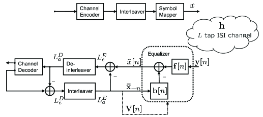
Figure 1: System block diagram for a bit interleaved coded modulation transmitter and receiver with a linear TEQ

For a linear equalizer with a feedforward filter ${f}$ and feedback filter ${b}$, an estimate of the transmitted signal can be given by

$$\hat{x}[n]=\mbox{\boldmath${f}$}^{H}[n]{\mathbf{y}}[n]-\mbox{\boldmath${b}$}^{H}[n]\bar{{\mathbf{x}}}_{-n}[n],$$ (1)

where $\mbox{\boldmath${y}$}[n]=[y[n-N_{2}],\cdots,y[n+N_{1}]]^{T}$, $\bar{{\mathbf{x}}}_{-n}[n]=[\bar{x}[n-N_{2}-L+1],\cdots,\bar{x}[n-1],\bar{x}[n+1],\cdots,\bar{x}[n+N_{1}]]^{T}$. The mean symbol values are calculated using the a priori information $L_{a}^{E}$ provided by the SISO decoder, i.e., $\bar{x}[n]=E[x[n]:\{L_{a}^{E}\}]$ and $E[|x[n]|^{2}:\{L_{a}^{E}\}]=1$ [1], where we assumed BPSK signaling for notational simplicity. If a linear MMSE equalizer is used in (1), we get

$${\mathbf{f}}[n]=({\mathbf{H}}_{-0}{\mathbf{V}}[n]{\mathbf{H}}_{-0}^{H}+{\mbox{\boldmath${s}$}}{\mbox{\boldmath${s}$}}^{H}+\sigma_{w}^{2}{\mathbf{I}})^{-1}{\mbox{\boldmath${s}$}},\mbox{\boldmath${b}$}[n]={\mathbf{H}}_{-0}^{H}{\mathbf{f}}[n],$$ (2)

where ${H}$ is the channel convolution matrix of size $N\times(N+L-1)$, ${s}$ is the $(N_{2}+L)$th column of ${\mathbf{H}}$, ${\mathbf{H}}_{-0}$ is the matrix where the $(N_{2}+L)$th column of ${\mathbf{H}}$ is eliminated, ${\mathbf{V}}[n]=\text{diag}([v[n-N_{2}-L+1],\cdots,v[n-1],v[n+1],\cdots,v[n+N_{1}]])$, $v[n]=E[|x[n]|^{2}:L_{a}^{E}]-|\bar{x}[n]|^{2}$ and $\sigma_{w}^{2}$ is the additive noise variance assuming fixed transmit signal power of $1$.

Remark 1

The linear MMSE equalizer in (2) is time varying due to the symbol-by-symbol variation of the soft input variance, ${\mathbf{V}}[n]$, even if $h_{l}$ is time invariant. The linear MMSE equalizer is a nonlinear function of ${\mathbf{V}}[n]$. If $h_{l}$ is also time varying, then (2) could be readily updated by including this time variation.

Unlike the linear MMSE equalizer, “direct” adaptive linear TEQs use adaptive updates (e.g. using LMS or RLS), for direct estimation of the transmitted symbols by processing the received signal and LLR information without the need for channel estimation [2]. In general, these approaches use only the mean vector $\bar{{\mathbf{x}}}_{-n}$ as feedback, i.e., soft decision data are not considered as a priori probabilities, where each component of $\bar{x}$ is taken as a random variable with zero mean and variance $\sigma_{\bar{x}}^{2}$. As an example, if one uses the NLMS direct adaptive linear equalizer, we have the update

$$e[n]=\tilde{x}[n]-{\mathbf{w}}^{H}[n]{\mathbf{u}}[n],{}$$

$${\mathbf{w}}[n+1]={\mathbf{w}}[n]+\mu e^{*}[n]{{\mathbf{u}}[n]}/{\|{\mathbf{u}}[n]\|^{2}},{}$$

where ${\mathbf{w}}[n+1]=[{\mathbf{f}}^{H}[n+1]\;-{\mathbf{b}}^{H}[n+1]]^{H}$, ${\mathbf{u}}[n]=[{\mathbf{y}}^{H}[n]\;\bar{{\mathbf{x}}}_{-n}^{H}]^{H}$, $\mu$ is the step size and $\tilde{x}[n]$ is equal to the mean $\bar{x}[n]$. Under this stationarity assumption on $\bar{x}$ and LLRs, the feedforward filter using $\bar{{\mathbf{x}}}_{-n}$ converges to the MSE optimal Wiener (stationary MMSE) solution

$${\mathbf{f}}=((1-\sigma_{\bar{x}}^{2}){\mathbf{H}}_{-0}{\mathbf{H}}_{-0}^{H}+{\mbox{\boldmath${s}$}}{\mbox{\boldmath${s}$}}^{H}+\sigma_{w}^{2}{\mathbf{I}})^{-1}{\mbox{\boldmath${s}$}}$$ (3)

and ${\mathbf{b}}={\mathbf{H}}_{-0}^{H}{\mathbf{f}}$, assuming zero variance at convergence [1]. The resulting filter in (3) at convergence is time invariant and is identical to (2) with time averaged soft information [1]. The linear MMSE in (2) requires $O((N+L)^{2})$ computations per output, however, (3) requires only $O(N+L)$. Since (3) is not time varying and implicitly assumes that the soft information is stationary, there is a large performance gap between linear MMSE in (2) and (3) [1]. We seek to reduce this performance gap between the direct adaptive methods with respect to the linear MMSE approach, by capturing the nonlinear dependence of the MMSE solution on the soft-information, without capturing the associated computational complexity of (2).

III Adaptive Turbo Equalization Using Hard or Soft Clustered Linear Models

We propose to use adaptive local linear filters to model the nonlinear dependence of the linear MMSE equalizer on the variance computed from the soft information generated by the SISO decoder in (2). We do this by partitioning the space of variances in (2) into a set of regions within each of which a single direct adaptive linear filter is used. As a result, we can retain the computational efficiency of the direct adaptive methods, while capturing the nonlinear dependence (and hence sample-by-sample variation) of the MMSE optimal TEQ.

III-A Adaptive Nonlinear Turbo Equalization Based on Hard Clustering

Suppose a hard clustering algorithm is applied to $\{\mbox{\boldmath${v}$}[n]\}_{n\geq 1}$ after the first turbo iteration to yield $K$ regions ${\mathcal{R}}_{k}$, with the corresponding centroids $\tilde{\mbox{\boldmath${v}$}}_{k}$, $k=1,\ldots,K$. Here, $\mbox{$\mbox{\boldmath${v}$}$}[n]$ is the vector formed by the diagonal entries of ${\mathbf{V}}[n]$. As an example, one might use the $K$-means algorithm (LBG VQ)[3]. In the LBG VQ algorithm, the centroids and the corresponding regions are determined as $\tilde{\mbox{$\mbox{\boldmath${v}$}$}}_{k}\stackrel{{\scriptstyle\bigtriangleup}}{{=}}\sum_{n,\mbox{$\mbox{\boldmath${v}$}$}[n]\in{\mathcal{R}}_{k}}\mbox{$\mbox{\boldmath${v}$}$}[n]/\left(\sum_{n,\mbox{$\mbox{\boldmath${v}$}$}[n]\in{\mathcal{R}}_{k}}1\right),$ and ${\mathcal{R}}_{k}\stackrel{{\scriptstyle\bigtriangleup}}{{=}}\{\mbox{$\mbox{\boldmath${v}$}$}:\|\mbox{$\mbox{\boldmath${v}$}$}-\tilde{\mbox{$\mbox{\boldmath${v}$}$}}_{k}\|\leq\|\mbox{$\mbox{\boldmath${v}$}$}-\tilde{\mbox{$\mbox{\boldmath${v}$}$}}_{i}\|,i=1,\ldots,K,i\neq k\}$, where the regions ${\mathcal{R}}_{k}$ are selected using a greedy algorithm [3]. After the regions are constructed using the VQ algorithm, the corresponding filters in each region are trained with an appropriate direct adaptive method, and the estimate of $x[n]$ at each time $n$ is computed as $\hat{x}[n]=\hat{x}_{i}[n]$ if $i=\arg\min_{k}\|\mbox{$\mbox{\boldmath${v}$}$}[n]-\tilde{\mbox{$\mbox{\boldmath${v}$}$}}_{k}\|$. For the adaptive algorithms to converge in each of these regions, we put a constraint on the cluster-size such that each cluster contains at least $N_{\min}$ (the minimum required data length for suitable convergence) elements and the quantization level is equal to or less than that of the original LBG VQ. At each time $n$, the received data is assigned to one of the regions and used in an adaptive algorithm to train a locally linear direct adaptive equalizer. For a locally NLMS direct adaptive linear equalizer, we have the update

$$e_{k}[n]=\tilde{x}[n]-{\mathbf{w}}_{k}^{H}[n]{\mathbf{u}}[n],$$ (4)

$${\mathbf{w}}_{k}[n+1]={\mathbf{w}}_{k}[n]+\mu e_{k}^{*}[n]{\mathbf{u}}[n]/(\|{\mathbf{u}}[n]\|^{2}),~{}{\mathbf{v}}[n]\in{\mathcal{R}}_{k},{}$$

$${\mathbf{w}}_{i}[n+1]={\mathbf{w}}_{i}[n],i=1,\ldots,K,i\neq k,$$ (5)

$$\hat{x}[n]=\hat{x}_{k}[n],{}$$

where ${\mathbf{w}}_{k}[n+1]=[{\mathbf{f}}_{k}^{H}[n+1]\;-{\mathbf{b}}_{k}^{H}[n+1]]^{H}$, ${\mathbf{u}}[n]=[{\mathbf{y}}^{H}[n]\;\bar{{\mathbf{x}}}_{-n}^{H}]^{H}$, and $\tilde{x}[n]$ in (4) is equal to either the hard quantized $\hat{x}[n]$ or the mean $\bar{x}[n]$ in decision directed (DD) mode. An algorithm description is given in Table I. Here, $L_{T}$ and $L_{D}$ are the length of training data and transmit data. During training period, perfect knowledge for the transmitted data $x[n]$ is available, so the $K$ adaptive filters can use weighted training symbols as input to the feedback filters in order to enable the filters to converge to a function of the quantized soft input variance. The weight matrices are selected as $(\mbox{\boldmath${I}$}-\tilde{\mbox{\boldmath${V}$}}_{k^{(i)}})$ at the $i$th turbo iteration.

TABLE I: Pseudocode for adaptive TEQ via hard clustering

Set $N_{\min}$. $K_{1}=\lfloor{L_{D}}/{N_{\min}}\rfloor$, (line A)

$i=1$, $\%$ First turbo iteration

for $k=1:K+1$; $\mbox{\boldmath${w}$}_{k^{(1)}}=\mbox{\boldmath${0}$}$, endfor

for $n=1:L_{T}$;

$e[n]=x[n]-\mbox{\boldmath${w}$}_{(k+1)^{(1)}}^{H}[n]{\mbox{\boldmath${u}$}}[n]$,

$\mbox{\boldmath${w}$}_{(k+1)^{(1)}}[n+1]=\mbox{\boldmath${w}$}_{(k+1)^{(1)}}[n]+\mu e^{*}[n]{\mbox{\boldmath${u}$}}[n]$, endfor

for $n=L_{T}+1:L_{T}+L_{D}$;

$e[n]=\tilde{x}[n]-\mbox{\boldmath${w}$}_{(k+1)^{(1)}}^{H}[n]{\mbox{\boldmath${u}$}}[n]$,

$\mbox{\boldmath${w}$}_{(k+1)^{(1)}}[n+1]=\mbox{\boldmath${w}$}_{(k+1)^{(1)}}[n]+\mu e^{*}[n]{\mbox{\boldmath${u}$}}[n]$, endfor

for $i=2,\ldots,$ $\%$ turbo iterations,

Perform hard clustering, based on modified LBG algorithm. (line B)

Outputs: $K_{i}=K$, $\mbox{\boldmath${V}$}_{k^{(i)}}=\mbox{\boldmath${V}$}_{k}$, (line C)

for $k^{(i)}=1:K_{i}$, $\%$ Filter initialization

if $i==2$; ${\mathbf{f}}_{k^{(i)}}[1]={\mathbf{f}}_{K_{1}+1}[L_{T}+L_{D}]$,

else $k^{*}=\underset{k^{(i-1)}}{\operatorname{argmin\,}}{\|\tilde{{\mathbf{V}}}_{k^{(i)}}-\tilde{{\mathbf{V}}}_{k^{(i-1)}}\|^{2}}$,

$k^{(i-1)}=1,\ldots,K_{i-1}$, ${\mathbf{f}}_{k^{(i)}}[1]={\mathbf{f}}_{k^{*}}[L_{T}+L_{D}]$,

${\mathbf{b}}_{k^{(i)}}[1]={\mathbf{b}}_{k^{*}}[L_{T}+L_{D}]$, endfor

for $n=1:L_{T}$, $\%$ Training period.

${\mbox{\boldmath${w}$}}_{k}[n+1]={\mbox{\boldmath${w}$}}_{k}[n]+\mu_{k}e_{k}^{*}[n]({\mathbf{I}}-\tilde{{\mathbf{V}}}_{k^{(i)}})^{1/2}\mbox{\boldmath${u}$}[n]$, endfor

for $n=L_{T}+1:L_{T}+L_{D}$;

$k^{*}=\underset{k^{(i-1)}}{\operatorname{argmin\,}}{\|\tilde{{\mathbf{V}}}_{k^{(i)}}-{{\mathbf{V}}}[n]\|^{2}}$ (line D)

${\mathbf{w}}_{k^{*}}[n+1]={\mathbf{w}}_{k^{*}}[n]+\mu_{k}[n]e_{k}^{*}[n]{{\mathbf{u}}[n]}/{\|{\mathbf{u}}[n]\|^{2}}$, (line E)

$\mu_{k}[n]=\left\{\begin{array}[]{l}{\mu\text{ for }k=k^{*}}\\ {0}\\ \end{array}\right.$, $\hat{x}[n]={\mathbf{w}}_{k^{*}}^{T}[n]{\mathbf{u}}[n]$ endfor (line F)

Go to the Clustering step: Until desired turbo iterations or error rate

Note that the complexity of the locally linear adaptive filters are higher than direct equalization due to the clustering step. Since the clustering is only performed at the start of each iteration with $O(N+L-1)$ complexity per data symbol, the equalization complexity is effectively unchanged per output symbol. If the regions are dense enough such that $\mbox{\boldmath${v}$}[n]\approx\tilde{\mbox{\boldmath${v}$}}_{k}$ for all regions, then the adaptive filter in the $k$th region converges to ${\mathbf{f}}_{k}=({\mathbf{H}}_{-0}\tilde{{\mathbf{V}}}_{k}{\mathbf{H}}_{-0}^{H}+{\mbox{\boldmath${s}$}}{\mbox{\boldmath${s}$}}^{H}+\sigma_{w}^{2}{\mathbf{I}})^{-1}{\mbox{\boldmath${s}$}},$ $\tilde{\mbox{\boldmath${V}$}}_{k}=\mathrm{diag}(\tilde{\mbox{\boldmath${v}$}}_{k})$, assuming zero variance at convergence. The difference between the MSE of the converged filter ${\mathbf{f}}_{k}$ and the MSE of the linear MMSE equalizer is given as [1]

$${\mathbf{f}}_{k}^{H}{\mathbf{H}}_{-0}({\mathbf{V}}[n]-\tilde{{\mathbf{V}}}_{k}){\mathbf{H}}_{-0}^{H}{\mathbf{f}}_{k}+(1-{\mathbf{f}}_{k}^{H}{\mbox{\boldmath${s}$}})-(1-{\mathbf{f}}_{n}^{H}{\mbox{\boldmath${s}$}}).\vspace{-0.05cm}$$ (6)

By defining ${\mathbf{A}}=({\mathbf{H}}_{-0}\tilde{{\mathbf{V}}}{\mathbf{H}}_{-0}^{H}+{\mbox{\boldmath${s}$}}{\mbox{\boldmath${s}$}}^{H}+\sigma_{w}^{2}{\mathbf{I}})$, ${\mathbf{B}}={\mathbf{A}}+{\mathbf{H}}_{-0}{\mathbf{E}}{\mathbf{H}}_{-0}^{H}$ and ${\mathbf{E}}={\mathbf{V}}-\tilde{{\mathbf{V}}}$, the difference (6) yields

$${\mbox{\boldmath${s}$}}^{H}{\mathbf{A}}^{-1}{\mathbf{H}}_{-0}{\mathbf{E}}{\mathbf{H}}_{-0}^{H}{\mathbf{A}}^{-1}{\mbox{\boldmath${s}$}}+{\mbox{\boldmath${s}$}}^{H}({\mathbf{B}}^{-1}-{\mathbf{A}}^{-1}){\mbox{\boldmath${s}$}}{}$$

$$={\mbox{\boldmath${s}$}}^{H}{\mathbf{A}}^{-1}{\mathbf{H}}_{-0}{\mathbf{E}}{\mathbf{H}}_{-0}^{H}{\mathbf{B}}^{-1}{\mathbf{H}}_{-0}{\mathbf{E}}{\mathbf{H}}_{-0}^{H}{\mathbf{A}}^{-1}{\mbox{\boldmath${s}$}}$$ (7)

$$\leq\lambda_{\mathrm{max}}({\mathbf{H}}_{-0}{\mathbf{E}}{\mathbf{H}}_{-0}^{H}{\mathbf{B}}^{-1}{\mathbf{H}}_{-0}{\mathbf{E}}{\mathbf{H}}_{-0}^{H}){\mbox{\boldmath${s}$}}^{H}{\mathbf{A}}^{-2}{\mbox{\boldmath${s}$}}$$ (8)

$$\leq e_{\mathrm{max}}^{2}\lambda_{\mathrm{max}}^{2}({\mathbf{H}}_{-0}{\mathbf{H}}_{-0}^{H}){\lambda_{\mathrm{min}}({\mathbf{B}})}{\mbox{\boldmath${s}$}}^{H}{\mathbf{A}}^{-2}{\mbox{\boldmath${s}$}}{},$$

where $e_{\mathrm{max}}$ is the maximum element of the error diagonal matrix ${\mathbf{E}}$. Here, (7) follows from $({\mathbf{B}}^{-1}-{\mathbf{C}}^{-1})={\mathbf{B}}^{-1}({\mathbf{C}}-{\mathbf{B}}){\mathbf{C}}^{-1}$, (8) follows from $\mathrm{tr}({\mathbf{C}}{\mathbf{D}})=\mathrm{tr}({\mathbf{D}}{\mathbf{C}})$ and $\mathrm{tr}({\mathbf{C}}{\mathbf{D}})\leq\lambda_{\mathrm{max}}({\mathbf{C}})\mathrm{tr}({\mathbf{D}})$, and the last line follows from $\lambda_{\mathrm{max}}({\mathbf{C}}{\mathbf{D}})\leq\lambda_{\mathrm{max}}({\mathbf{C}})\lambda_{\mathrm{max}}({\mathbf{D}})$. Since $\lambda_{\mathrm{min}}({\mathbf{B}})\geq\sigma_{w}^{2}$ and $\lambda_{\mathrm{max}}({\mathbf{H}}_{-0}{\mathbf{H}}_{-0}^{H})\leq\lambda_{\mathrm{max}}({\mathbf{H}}{\mathbf{H}}^{H})\leq(\sum_{m}{|h_{m}|})$ for the Toeplitz matrix ${\mathbf{H}}$, the MSE difference in (6) is bounded by $Ce_{\mathrm{max}}^{2}$ for some $C<\infty$. Hence, the MSE of the hard clustered linear equalizer converges to the MSE of the linear MMSE equalizer as the number of the regions increase provided there is enough data for training.

III-B Adaptive Nonlinear Turbo Equalization Based on Soft Clustering

Suppose the deterministic annealing (DA) algorithm described in Table II is used for soft clustering [3] on $\{\mbox{\boldmath${v}$}[n]\}_{n\geq 1}$ after the first turbo iteration, to give $K$ clusters with the corresponding centroids $\tilde{\mbox{\boldmath${v}$}}_{k}$ and association probabilities $P(v[n]|\tilde{\mbox{\boldmath${v}$}}_{k})$, $k=1,\ldots,K$. Then, at each time $n$, the vector $\mbox{\boldmath${v}$}[n]$ can be partially assigned to all $K$ regions using conditional probabilities yielding the update

$$e_{k}[n]=\tilde{x}[n]-\mbox{\boldmath${w}$}_{k}^{H}[n]\mbox{\boldmath${u}$}[n],{}$$

$${\mathbf{w}}_{k}[n+1]={\mathbf{w}}_{k}[n]+\mu_{k}[n]e_{k}^{*}[n]{\mathbf{u}}[n]/(\|{\mathbf{u}}[n]\|^{2}),$$ (9)

$$\mu_{k}[n]=\mu P\left({\mathbf{v}}[n]|\tilde{{\mathbf{v}}}_{k}\right),$$ (10)

where ${\mathbf{w}}_{k}[n+1]=[{\mathbf{f}}_{k}^{H}[n+1]\;\;-{\mathbf{b}}_{k}^{H}[n+1]]^{H}$, ${\mathbf{u}}[n]=[{\mathbf{y}}^{H}[n]\;\;\bar{{\mathbf{x}}}_{-n}^{H}]^{H}$ and $\mu_{k}[n]$ is the fractional step size. To generate the final output, outputs of $K$ linear filters can be combined by either using another adaptive algorithm [4] or other combination methods [3]. We use the method in [4] as follows. At each time $n$, we construct $\mbox{\boldmath${y}$}[n]=[\hat{x}_{1}[n],\ldots,\hat{x}_{K}[n]]^{T}$ and produce the final output and update the weight vectors as

$$\hat{x}[n]=\mbox{\boldmath${w}$}^{T}[n]\mbox{\boldmath${y}$}[n],$$ (11)

$$e[n]=\tilde{x}[n]-\mbox{\boldmath${w}$}^{T}[n]\mbox{\boldmath${y}$}[n],$$ (12)

$${\mathbf{w}}[n+1]={\mathbf{w}}[n]+\mu[n]e^{*}[n]{\mbox{\boldmath${y}$}[n]}/{\|\mbox{\boldmath${y}$}[n]\|^{2}},$$ (13)

and $\mu$ is a learning rate for this combining step. An update as in (13) can provide improved steady-state MSE and convergence speed exceeding that of any of the constituent filters, i.e., $\hat{x}_{k}[n]$, $k=1,\ldots,K$, under certain conditions [4].

The algorithm description is the same as in Table I, except that line A is removed and $K_{1}$ is set to $K_{\mathrm{max}}$, and soft clustering [3] is used in line B. In line C, we add an $L_{D}\times K_{i}$ probability matrix corresponding to $P\left({\mathbf{v}}[n]|\tilde{{\mathbf{v}}}_{k}\right)$ to the outputs. Line D and E are removed, (9) and (10) for all $k$ are used instead. Line F is also removed and replaced by (11), (12) and (13), respectively.

TABLE II: Soft Clustering based on Deterministic Annealing

$\%$ Set the maximum number of code vectors, the maximum number of iterations

$\%$ and a minimum temperature, i.e., $K_{\mathrm{max}}$, $I_{\mathrm{max}}$ and $T_{\mathrm{min}}$.

$K=1$, $\tilde{{\mathbf{v}}}_{1}=\frac{1}{N}\sum_{n}{\mathbf{v}}[n]$ and $P(\tilde{{\mathbf{v}}}_{1})=1$.

$T=T_{0}$ $\%$ An initial temperature, $T_{0}$, should be larger than $\lambda_{\mathrm{max}}\left(\mathrm{cov}\left({\mathbf{v}},{\mathbf{v}}\right)\right)$.

for $n=1:N$;   $P(\tilde{{\mathbf{v}}}_{k}|{\mathbf{v}}[n])=\frac{1}{N}$ endfor

$D=\frac{1}{N}\sum_{n}{d({\mathbf{v}}[n],\tilde{v}_{1})}$

if $T\geq T_{\min}$;

$T=aT$ for $a<1$ $\%$ Cooling Step

if $K\leq K_{\mathrm{max}}$; $j=0$.

for $k=1:K$;

if $T>Tc_{k}$; $\%$ Split the $k$th cluster with slight perturbation

elseif $j=j+1$ endfor

if $j==K$; finish DA.

elseif; finish DA

elseif; finish DA

$i=1$

while converged or $i<I_{\mathrm{max}}$;

for $k=1:K$;

for $n=1:N$;

$P(\tilde{{\mathbf{v}}}_{k}|{\mathbf{v}}[n])=P(\tilde{{\mathbf{v}}}_{k})exp(-\frac{\|{\mathbf{v}}[n]-\tilde{{\mathbf{v}}}_{k}\|^{2}}{T})/\sum_{k}{P(\tilde{{\mathbf{v}}}_{k})exp(-\frac{\|{\mathbf{v}}[n]-\tilde{{\mathbf{v}}}_{k}\|^{2}}{T})}$

$P(\tilde{{\mathbf{v}}}_{k})=\sum_{n}P({\mathbf{v}}[n])P(\tilde{{\mathbf{v}}}_{k}|{\mathbf{v}}[n])$, $\tilde{{\mathbf{v}}}_{k}=\frac{\sum_{n}{{\mathbf{v}}[n]P\left(\tilde{{\mathbf{v}}}_{k}|{\mathbf{v}}[n]\right)P\left({\mathbf{v}}[n]\right)}}{P\left(\tilde{{\mathbf{v}}}_{k}\right)}$

endfor $\%$ calculate distortion and check convergence

endwhile $\%$ Go to Cooling Step

IV Simulation Results

Throughout the simulations, a time invariant ISI channel given by $h_{l}=[0.227,0.46,0.688,0.46,0.227]$ is used. We use rate $1/2$ convolutional code with constraint length $3$, random interleaving and BPSK signaling. We choose $L_{T}=1024$, $L_{D}=4096$, $N_{\mathrm{min}}=500$ and $K_{\mathrm{max}}=8$. Each NLMS filter has a length 15 feedforward and length 19 feedback filter ($N_{1}=9,N_{2}=5$) where $\mu=0.03$. For an NLMS filter with soft clustered TEQ, the filter length is less than $K_{\mathrm{max}}$ and $\mu=0.1$. Fig. 4 and Fig. 4 show EXIT charts for a conventional NLMS TEQ [2] (LMSTEQ), the switched NLMS TEQ based on hard clustering with restriction on the number of data samples in each cluster (QLMSTEQ) and an NLMS TEQ based on soft clustering (SQLMSTEQ). In Fig. 4, hard decision data are used to learn the NLMS filter, while in Fig. 4 the transmitted signals are used during data the data transmission period. In Fig. 4, we provide the corresponding BERs.

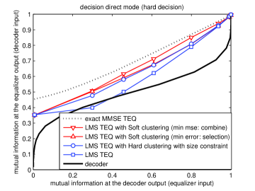
Figure 2: EXIT chart comparison in DD mode. ($Eb/N0=10dB$)

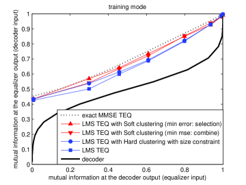
Figure 3: EXIT chart comparison in training mode. ($Eb/N0=10dB$)

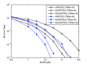
Figure 4: BER comparison in DD mode, where soft decision value from the decoder is used and TBiter is the turbo iteration count.

For the soft clustering based NLMS TEQ, the final output is given by either adaptively combining to minimize combined MSE with another NLMS filtering as given in Section III-B or selecting one of the outputs to minimize instantaneous residual error after filtering.

In all simulations, adaptive TEQs based on soft clustering showed significantly better performance to hard clustered adaptive TEQ and direct adaptive TEQ. In Fig. 4, (i.e., in the DD mode with hard decision data), the adaptive combination of adaptive filters showed better performance than selecting a single filter, since the combination method can mitigate the worst-case selection [4]. However, in a dynamically changing feature domain, combining the outputs of the constituent filters in MSE can loose the benefit from the local linear models [4]. As shown in Fig. 4, selecting one filter among $K$ filters shows better performance than the combination of the filters. As discussed in Section III, the DD-NLMS TEQ can achieve “ideal” performance, i.e. time-average MMSE TEQ, as the decision data becomes more reliable. However, there is still a mutual information gap between the exact MMSE TEQ and the NLMS adaptive TEQ. As an example, the NLMS TEQ in Fig. 4 cannot converge to its ideal performance if the tunnel between the transfer function of equalizer and that of the decoder is closed. This point can be identified by measuring the signal to noise ratio (SNR) threshold. If the SNR is higher than the SNR threshold, turbo equalization can converge to near error-free operation. Otherwise, turbo equalization stalls, and fails to improve after a few iterations. The $\frac{Eb}{N0}$s corresponding to the SNR thresholds by equalization algorithm are given in Table III. Adaptive nonlinear TEQs based on soft clustering yielded $0.5dB\frac{Eb}{N0}$ gain in SNR threshold compared to adaptive nonlinear TEQ based on hard clustering and about $1dB\frac{Eb}{N0}$ gain compared to the conventional adaptive linear TEQ.

TABLE III: SNR thresholds in $dB$ of several algorithms

mode	decision directed	training
original NLMS TEQ	10.9	6.0
NLMS TEQ w/ hard clustering	6.5	5.5
NLMS TEQ w/ soft clustering (combine)	5.3	5.0
NLMS TEQ w/ soft clustering (selection)	5.9	4.8

V Conclusion

We introduced adaptive locally linear filters based on hard and soft clustering to model the nonlinear dependency of the linear MMSE turbo-equalizer on soft information from the decoder. The adaptive equalizers have computational complexity on the order of an ordinary direct adaptive linear equalizer. The local adaptive filters are updated either based on their associated region using hard clustering or fractionally based on association probabilities in soft clustering. Through simulations, the superiority of the proposed algorithms are demonstrated.

References

• [1] M. Tüchler, R. Koetter, and A. Singer, “Turbo equalization: principles and new results,” IEEE Trans. Commun., vol. 50, no. 5, pp. 754–767, May 2002.
• [2] C. Laot, A. Glavieux, and J. Labat, “Turbo equalization: adaptive equalization and channel decoding jointly optimized,” IEEE Jour. Select. Areas in Commun., vol. 19, no. 9, pp. 1744–1752, Sep 2001.
• [3] A. Gersho and R. M. Gray, Vector Quantization and Signal Compression.   Kluwer Academic Pub. Co., 1992.
• [4] S. S. Kozat, A. E. Erdogan, A. C. Singer, and A. H. Sayed, “Steady-state MSE performance analysis of mixture approaches to adaptive filtering,” IEEE Trans. Sig. Proc., vol. 58, pp. 4050–4063, Aug. 2010.