Clustering Using Isoperimetric Number of Trees

Abstract

In this paper we propose a graph-based data clustering algorithm which is based on exact clustering of a minimum spanning tree in terms of a minimum isoperimetry criteria. We show that our basic clustering algorithm runs in $O(n\log n)$ and with post-processing in $O(n^{2})$ (worst case) time where $n$ is the size of the data set. We also show that our generalized graph model which also allows the use of potentials at vertices can be used to extract a more detailed pack of information as the outlier profile of the data set. In this direction we show that our approach can be used to define the concept of an outlier-set in a precise way and we propose approximation algorithms for finding such sets. We also provide a comparative performance analysis of our algorithm with other related ones and we show that the new clustering algorithm (without the outlier extraction procedure) behaves quite effectively even on hard benchmarks and handmade examples.

I Introduction

I-A A concise survey of main results

Data clustering, as the unsupervised grouping of similar patterns into clusters, is a central problem in engineering disciplines and applied sciences which is also constantly under theoretical and practical development and verification. In this article we are concerned with graph based data clustering methods which are extensively studied and developed mainly because of their simple implementation and acceptable efficiency in a number of different fields as signal and image processing, computer vision, computational biology, machine learning and networking to name a few.

The main contribution in this article can be described as a general graph-based data clustering algorithm which falls into the category of such algorithms that use a properly defined sparsest cut problem as the clustering criteria. In this regard, it is instructive to note some highlights of our approach before we delve into the details in subsequent sections (details of our approach as well as a survey of related contributions will appear in the second part of this introduction).

It has been already verified that graph-based clustering methods that operate in terms of non-normalized cuts are not suitable for general data clustering and behave poorly in comparison to the normalized versions (e.g. see [29]). Moreover, it is well known that there is a close relationship between the minimizers of the normalized cut problem, spectral clustering solutions, mixing rates of random walks, the minimizers of the K-means cost function, kernel PCA and low dimensional embedding, while the corresponding decision problems are known to be NP-complete in general (e.g. see [5, 4, 1, 19, 24, 3] and references therein).

In this article, we will provide an efficient clustering algorithm which is based on a relaxation of the feasible space of solutions from the set of partitions to the larger set of subpartitions (i.e. mutually disjoint subsets of the domain). From one point of view, our algorithm can be considered as a generalization of Grady and Schwartz approach [11, 10] based on isoperimetry problems while we extensively rely on the results of [5] and [4]. Also, we believe that this relaxation which is based on moving from the space of partitions to the space of subpartitions not only provides a chance of making the problem easier to solve but also is in coherence with the natural phenomena of having undesirable data or outliers. We will use this property to show that our algorithm can be enhanced to a more advanced procedure which is capable of presenting a hierarchy of data similarity profile which can lead to the extraction of outliers.

In this regard, one may comment on some different aspects of this approach as follows.

Theoretical aspects: From a theoretical point of view, it is proved in [4] that the normalized cut criteria is not formally well defined in the sense that it does not admit a variational description through a real function relaxation of the problem (i.e. it does not admit a Federer-Fleming type theorem). However, for $k\geq 2$, the well-defined version, known as the $k$-isoperimetry problem (defined in [4]), whose definition is in terms of normalized-flow minimization on $k$-subpartitions, actually admits such a relaxation. It should be noted that although there are some approaches to clustering which are based on the classical $2$-isoperimetry (i.e. Cheeger constant) on weighted graphs (e.g. see [11]), but as it follows from the results of [4], in the classical model the difference between the cases of partitions and subpartitions only is observable when $k\geq 3$, and consequently, our approach is completely different in nature from iterative $2$-partitioning or spectral approximation methods based on eigenmaps already existing in the literature.

Also, as a bit of a surprise (see Theorem 1), it turns out that a special version of the $k$-isoperimetry problem is efficiently solvable for trees. This fact along with a well-known approach of finding an approximate graph partitioning through minimum spanning trees constitute the core of our algorithm.

Practical aspects: There are different practical aspects of the proposed algorithm that one may comment on. Firstly, the proposed approximation algorithm run-time is almost linear in terms of the size of input-data which provides an opportunity to cluster large data sets. Also, it should be noted that our algorithm for $k$-clustering obtains an exact optimal clustering of a suitably chosen subtree in a global approach and does not apply an iterative two-partitioning or an approximation through eigenmaps. This in a way is one of the reasons supporting a better approximation of our algorithm compared to the other existing ones. In this regard, we also present a number of experimental results justifying a better performance of our algorithm in practice (see Tables I, II and Section III).

Secondly, we should note that approximation through the isoperimetry criteria provides an extra piece of information as a (possibly nonempty) subset of the domain (since the union of subpartitions may not be a covering). This piece of information makes it possible to obtain the almost minimal clustering as well as to extract deviated data and outliers, at the same time. In order to handle this extra information, we have generalized our graph model to the case of a weighted graph with potential. This generalization of the graph representation model is another original aspect of our contribution where we rely on results of [5] and [4] in this more general setting (see Theorem 1). It is interesting to note that in this more general setting our results presented in Section IV show that not only we can handle the case of outlier extraction with clustering at the same time, but also the new set up will make it possible to extract outliers even in the case of $2$-clusterings (which is theoretically meaningless by definition when one is using the classical isoperimetry or $2$-normalized cuts). Using this setting we propose a formal definition for the outlier profile of a data set and, moreover, we provide a couple of examples to study the efficiency of the proposed method in extracting outliers.

I-B Background and related contributions

Unsupervised grouping of data based on a predefined similarity criteria is usually referred to as data clustering in general, where in some more specific applications one may encounter some other terms as segmentation in image processing or grouping in data mining. Based on its importance and applicability, there exists a very vast literature related to this subject (e.g. see [13, 6] for some general background), however, in this article we are mainly concerned with clustering algorithms that rely on a representation of data as a simple weighted graph in which the edge-weights are tuned, using a predefined similarity measure (e.g. see Section II, [28] and references therein).

Graph-based data clustering is usually reduced to the graph partitioning problem on the corresponding weighted graph which is also well-studied in the literature. To this end, it is instructive to note that from this point of view and if one considers a weighted graph as a geometric object, then the partitioning problem can be linked to a couple of very central and extensively studied problems in geometry as isoperimetry problem, concentration of measure and estimation of diffusion rates (e.g. see [4, 1] and references therein).

A graph-based clustering or a graph partitioning problem is usually reduced to an optimization problem where the cost function is a measure of sparsity or density related to the corresponding classes of data. From this point of view, it is not a surprise to see a variety of such measures in the literature, however, from a more theoretical standpoint such similarity measures are well-studied and, at least, the most geometrically-important classes of them are characterized (e.g. see [27] for a very general setting). In this context such measures usually appear as norms or their normalized versions that should be minimized or maximized to lead to the expected answer.

What is commonly refereed to as spectral clustering is the case in which the corresponding normalized norm is expressed as an $L^{2}$ (i.e. Euclidean) norm and admits a real-function relaxation whose minimum is actually an eigenvalue of the weight (or a related) matrix of the graph. This special case along with the important fact that, the spectral properties (i.e. eigenvalues and eigenfunctions) of a finite matrix can be effectively (at most in $O(n^{3})$ time) computed, provides a very interesting setting for data clustering in which the corresponding optimization problem can be tackled with using the well-known tools of linear algebra and operator theory (e.g. see [17, 22, 21, 33, 31, 16, 20, 35] and references therein for a general background in spectral methods).

Although, applying spectral methods are quite effective and vastly applied in data clustering, but still the time complexity of the known algorithms and also the approximation factor of this approach in not as good as one expects when one is dealing with large data sets (e.g. see [26] that proves an approximation factor of at most $2$). On the other way round, these facts leads one to consider the original normalized versions of the $L^{1}$ norm that reduces clustering to the sparsest (or similar minimal) cut problems or their real-function relaxations as the corresponding approximations. It is proved in [4] that the most natural such normalized norms do not admit real-function relaxations when they are minimized over partitions of their domain. Moreover, it is shown in the same reference that such normalized norms do admit such real-function relaxations when they are minimized over subpartitions of their domain. In this new setting the minimum values, that correspond to the eigenvalues in the spectral $L^{2}$ setting, are usually referred to as isoperimetric constants.

Unfortunately, contrary to the case of $L^{2}$, decision problems corresponding to the isoperimetry problems are usually NP-hard (e.g. see [29, 5, 19, 15]), which shows that computing the exact value of the isoperimetric constants is not an easy task. There has been a number of contributions in the literature whose main objectives can be described as to proposing different methods to get around this hardness problem and find an approximation for the corresponding isoperimetry problem as a criteria of clustering, and consequently, obtaining an approximate clustering of the given data.

In this regard, one may at least note two different approaches as follows. In the one hand, there has been contributions who has tried to reduce the problem to the more tractable case of trees by first finding a suitable subtree of the graph and then try to approximately cluster the tree itself (e.g. see [2, 25, 12, 18, 8, 34, 32]). The difference between such contributions usually falls into the way of choosing the subtree and the method of their clustering. On the other hand, one may also try to obtain a global clustering by a mimic of spectral methods through solving not an eigenfunction problem but a similar problem in $L^{1}$ (e.g. see [11, 10]). These methods usually follow an iterative $2$-partitioning since there was not much information about approximations for higher order eigenfunctions or similar solutions in $L^{1}$ until recently (e.g. see [19, 11]).

Our main contribution in this article can be described as a culmination of above mentioned ideas that strongly rely on some recent studies of higher order solutions of isoperimetry problems (see [5, 4]), in which we first search for a suitable spanning subtree and after that we obtain the exact solution of the corresponding optimization problem for our suitably chosen isoperimetric constant (see Section II). Also, in this setting we will obtain a subset of unused data given as the complement of the obtained clustering as a subpartition and we will try to analyze this extra output of our algorithm as an outlier detection procedure (see Section IV). To do this we adopt a generalize graph model as a weighted graph with potential and we will be needing a generalization of some results of [5] and [4] that will be presented in Section II. Also, in Sections III and IV we provide experimental results to show the efficiency and the performance of our proposed algorithms.

II The clustering model and algorithm

In this section we introduce our graph based model and the proposed clustering algorithm.

Fix positive integers $d\geq 1$, $k$ and $n$ such that $2\leq k\leq n$ and let $X=\{x_{1},\ldots,x_{n}\}$ be a set of $n$ vectors in $\mathbb{R}^{d}$. A standard $k$-clustering problem for $X$ is to find a $k$-partition of $X$ with a high intra-clusters similarity as well as a low inter-clusters similarity (with respect to a predefined similarity measure).

In graph-based methods of clustering, the data-set $X$ is represented by a weighted graph on $n$ vertices, where each vertex corresponds to a vector in $X$ and the weight of an edge $x_{i}x_{j}$ reflects the similarity between vectors $x_{i}$ and $x_{j}$. In this article, our graph model consists of a simple graph $G=(X,E)$ on the vertex set $X:=\{x_{1},\ldots,x_{n}\}$ endowed with three weight functions, namely, a vertex-weight function $\omega:X\to\mathbb{R}^{+}$, an edge-weight function $\varphi:E\to\mathbb{R}^{+}$ called the flow and a function $p:X\to\mathbb{R}$ called the potential. The function $\omega$ is used for the weight of each element of the data-set $X$ and the similarities between pairs of elements are denoted by the flow function $\varphi$. The potential of a vertex $x_{i}\in X$, $p(x_{i})$, is used to represent the extent of isolation or alienation of $x_{i}$ from other elements. In this setting, the weighted graph is called the similarity or affinity graph and is denoted by $(G,\omega,\varphi,p)$ where, hereafter, the size of the data-set which is equal to the number of vertices is fixed to be $n:=|X|$. For instance, in a classic way of modelling similarities, one may define the flow and vertex weight functions as follows,

$$\begin{split}\forall\ 1\leq i\neq j\leq n,\ \varphi(x_{i}x_{j})&:=\exp(-\|x_{i}-x_{j}\|_{{}_{2}}/2\sigma^{2}),\\ \forall\ \leq i\leq n,\ \omega(x_{i})&:=\sum_{j=1}^{n}\varphi(x_{i}x_{j}).\end{split}$$ (1)

We do not elaborate on the more or less complex subject of proposing suitable methods for graphical presentation of data sets. The interested reader is referred to the existing literature (e.g. [36]) to see how the scale parameter $\sigma$ is chosen and how it affects the performance of graph based algorithms. However, in order to present a complete comparison in Section III we consider both global scaling and local scaling models in our performance analysis.

In the sequel we will discuss the important role of potentials in Section IV, when we elaborate on the capability of our algorithm to detect the outlier profile of the data set.

To describe our model of clustering, first we need to define a couple of notations. For a subset $A\subset X$, the boundary of $A$, denoted by $\partial A$, is defined as,

$$\partial A:=\{e=xy\in E\ |\ x\in A,y\in X\setminus A\}.$$

Also, for any given finite set $A$, a function $f:A\to\mathbb{R}$ and a subset $B\subseteq A$, we define

$$f(B):=\sum_{x\in B}f(x).$$

The collection of all $k$-partitions of the set $X$ is denoted by $\mathscr{P}_{k}(X)$. Given a weighted graph $(G,\omega,\varphi,p)$ and an integer $2\leq k\leq n$, (the maximum version of) the $k$-normalized cut problem seeks for a $k$-partition $\mathcal{A}:=\{A_{1},\ldots,A_{k}\}\in\mathscr{P}_{k}(X)$ that minimizes the following cost function,

$${\rm cost}(\mathcal{A}):=\max_{1\leq i\leq k}\frac{\varphi(\partial A_{i})+p(A_{i})}{\omega(A_{i})}.$$ (2)

We define

$${\rm MNC}_{k}(G):=\min_{\mathcal{A}\in\mathscr{P}_{k}(X)}{\rm cost}(\mathcal{A}).$$

The quotient ${(\varphi(\partial A_{i})+p(A_{i}))}/{\omega(A_{i})}$ is called normalized flow of the set $A_{i}$. The (max) normalized cut problem is known to be $NP$-hard for general graphs even when $k=2$ [23]. In [5] the same problem is investigated for weighted trees and it is proved that the corresponding decision problem for arbitrary $k$ remains $NP$-complete even for simple (unweighted) trees. In the same reference a tractable relaxation of the problem is also proposed which is based on the relaxation of the feasible set from the set of $k$-partitions to the set of $k$-subpartitions, i.e. $k$ disjoint subsets of the vertex set. The set of all $k$-subpartitions of $X$, denoted by $\mathscr{D}_{k}(X)$, is defined as follows,

$$\mathscr{D}_{k}(X):= \{\mathcal{A}:=\{A_{1},\ldots,A_{k}\}\ |\$$

$$\forall\ i,A_{i}\subset X,{\rm and}\ \forall\ i\neq j,A_{i}\cap A_{j}=\emptyset\}.$$

For a subpartition $\mathcal{A}=\{A_{1},\ldots,A_{k}\}\in\mathscr{D}_{k}(X)$, each element in $X\setminus\cup_{i=1}^{k}A_{i}$ is called a residue element (w.r.t. $\mathcal{A}$) and the number of residue elements is called the residue number of $\mathcal{A}$.

The (maximum version) of isoperimetric problem seeks for a minimizer of the cost function in (2) over the space of all $k$-subpartitions of $X$. We denote the minimum by ${\rm MISO}_{k}(G)$, i.e.

$${\rm MISO}_{k}(G):=\min_{\mathcal{A}\in\mathscr{D}_{k}(X)}{\rm cost}(\mathcal{A}).$$

It is not hard to check that there exist instances where the minimum ${\rm MISO}_{k}(G)$ occurs on a subpartition which is not actually a partition, and also it can be verified that ${\rm MNC}_{2}(G)={\rm MISO}_{2}(G)$ when the potential function is equal to zero (see [4]).

The idea of relaxing the normalized cut problem to the isoperimetric problem have a number of justifications from different points of view. On the one hand, from a computational viewpoint, the isoperimetric problem is more tractable in some special cases (e.g. see Theorem 1), while, on the other hand, from a theoretical viewpoint, it can be verified that the isoperimetry problem admits a Federer-Fleming-type theorem, while the normalized cut problem doesn’t satisfy such a relaxation in general (see Theorem II and [4]).

For two given real functions $f$ and $g$ on $X$ and a positive weight fuction $\omega:X\to\mathbb{R}^{+}$ define the weighted inner product as

$$\langle f_{i},f_{j}\rangle_{\omega}:=\displaystyle{\sum_{x\in X}}f(x)g(x)\omega(x).$$

Also, if $\mathscr{F}^{+}(X)$ is the set of all non-negative real functions on $X$ and $k>1$ is a positive integer, $\mathscr{O}_{{}_{k}}^{+}(X)$ stands for the set of $k$ mutually orthogonal functions in $\mathscr{F}^{+}(X)$, i.e.

$$\mathscr{O}_{{}_{k}}^{+}(X) :=\{\{f_{1},\ldots,f_{k}\}\ |\ f_{i}\in\mathscr{F}^{+}(X),$$

$$\quad\quad\quad\langle f_{i},f_{j}\rangle_{\omega}=0,\ \forall\ i\neq j\}.$$

Now, one may verify that the following Federer-Fleming-type theorem holds. We deliberately exclude the proof since it is essentially a straight forward generalization of the proof already presented in [4] for the standard case (i.e. when the potential function is equal to zero).

Theorem 1[14].
For every weighted graph $(G,\omega,\varphi,p)$ and integer $k$,

$$\begin{split}{\rm MISO}&{}_{k}(G)=\displaystyle{\inf_{\{f_{i}\}^{k}_{1}\in{\mathscr{O}}^{+}_{k}(G)}}\ \max_{1\leq i\leq k}\\[5.0pt] &\left(\frac{\displaystyle\sum_{xy\in E}\varphi(xy)\ |f_{i}(x)-f_{i}(y)|+\sum_{x\in V}p(x)\ |f_{i}(x)|}{\displaystyle\sum_{x\in V}\omega(x)\ |f_{i}(x)|}\right)\end{split}$$

It is shown in [5] that in the case of weighted trees, despite intractability of the normalized cut problem, the decision problem related to ${\rm MISO}_{k}(G)$ is efficiently solvable in the following sense.

Theorem 2[5].
For every weighted tree $(T,\omega,\varphi,p)$, the decision version of the (max) isoperimetry problem can be efficiently solved in linear time.

Since our proposed clustering method is based on the algorithm announced in Theorem II, we include the algorithm for completeness (see Algorithm 1). In what follows assume that a vertex $v$ is selected as the root and the vertices are ordered in a BFS order, as $x_{1},\ldots,x_{n}=v$.

Algorithm 1 Given a weighted tree $(T,\omega,\varphi,p)$, an integer $k$ and a rational number $N$, decide whether there exists some $\mathcal{A}\in\mathscr{D}_{k}(X)$ such that ${\rm cost}(\mathcal{A})\leq N$ as in (2).

  Initialize the set function $\eta:X\to\mathcal{P}(X)$ by $\eta(x_{i}):=\{x_{i}\}$ for each $1\leq i\leq n$.

  Define $i=j:=1$.

  while $j<k$ and $i\leq n$ do

     Let $u$ be the unique parent of $x_{i}$ and $e:=ux_{i}\in E$ (if $i=n$, then define $\varphi(e):=0$)

     if $p(x_{i})+\varphi(e)\leq N\omega(x_{i})$ then

        $j\leftarrow j+1$, $A_{j}\leftarrow\eta(x_{i})$,

        $\omega(A_{j})\leftarrow\omega(x_{i})$,

        $\varphi(\partial A_{j})\leftarrow\varphi(e)+p(x_{i})$,

        $p(u)\leftarrow p(u)+\varphi(e)$.

     else if $p(x_{i})-\varphi(e)<N\omega(x_{i})$ then

        $\eta(u)\leftarrow\eta(u)\cup\eta(x_{i})$,

        $\omega(u)\leftarrow\omega(u)+\omega(x_{i})$,

        $p(u)\leftarrow p(u)+p(x_{i})$.

     else {i.e. $p(x_{i})-\varphi(e)\geq N\omega(x_{i})$}

        $p(u)\leftarrow p(u)+\varphi(e)$

     end if

  end while

  if $j=k$ then

     

     return  YES and $\{A_{1},\ldots,A_{k}\}$

  else

     

     return  NO

  end if

In this article we provide an improved version of Theorem II as follows.

Theorem 3.
For every weighted tree $(T,\omega,\varphi,p)$ on $n$ vertices and every integer $2\leq k\leq n$, the value of ${\rm MISO}_{k}(T)$ and a minimizer in $\mathscr{D}_{k}(V)$ can be found in time $O(n\log n)$.

Proof:

Let $T=(V,E,\omega,\varphi,p)$ be a fixed weighted tree on $n$ vertices and $1\leq k\leq n$ be a fixed integer. Without loss of generality, assume that all the weights are integer. Define

$$\omega_{*}:=\min_{x\in V}\omega(x),\quad\omega^{*}:=\sum_{x\in V}\omega(x),$$

$$\varphi_{*}:=\min_{e\in E}\varphi(e),\quad\varphi^{*}:=\sum_{e\in E}\varphi(e),$$

$$p_{*}:=\min_{x\in V}p(x)\ \ {\rm and}\ \ p^{*}:=\sum_{x\in V}p(x).$$

Note that for every non-empty subset $A\subsetneq V$, the value of ${(\varphi(\partial A)+p(A))}/{\omega(A)}$ is a rational number within the interval $[{(\varphi_{*}+p_{*})}/{\omega^{*}},{(\varphi^{*}+p^{*})}/{\omega_{*}}]$. Furthermore, for two non-empty subsets $A,B\subsetneq V$, if $a:={(\varphi(\partial A)+p(A))}/{\omega(A)}$ and $b:={(\varphi(\partial B)+p(B))}/{\omega(B)}$ are distinct, then

$$|a-b|\geq\frac{\varphi_{*}+p_{*}}{{\omega^{*}}^{2}}.$$ (3)

Based on Algorithm 1, Algorithm 2 described below, finds a minimizer for ${\rm MISO}_{k}(T)$.

Input: data-set $X$ and integer $k>1$ $\stackrel{{\scriptstyle\rm\phantom{Approx.}}}{{\longrightarrow}}$ Pre-process: generate the affinity graph $G$ $\stackrel{{\scriptstyle\rm Approx.}}{{\longrightarrow}}$ Find: a minimum spanning tree $T$ $\stackrel{{\scriptstyle\rm Exact}}{{\longrightarrow}}$ Compute: ${\rm MISO}_{k}(T)$ and a minimizing subpartition $\stackrel{{\scriptstyle\rm Approx.}}{{\longrightarrow}}$ Post-process: reduce the residue number

Figure 1: An outline of the main algorithm.

Algorithm 2 Given a weighted tree $(T,\omega,\varphi,p)$ and an integer $k$, find a minimizer achieving ${\rm MISO}_{k}(T)$.

  Let $\alpha_{0}\leftarrow\frac{\varphi_{*}+p_{*}}{\omega^{*}}$ and $\beta_{0}\leftarrow\frac{\varphi^{*}+p^{*}}{\omega_{*}}$.

  Let $t\leftarrow\log({2{\omega^{*}}^{2}(\beta_{0}-\alpha_{0}}))-\log({\varphi_{*}+p_{*}})$.

  Initialize $\alpha\leftarrow\alpha_{0}$ and $\beta\leftarrow\beta_{0}$.

  for $i=1$ to $t$ do

     Applying Algorithm 1, decide if ${\rm MISO}_{k}(T)\leq\frac{\alpha+\beta}{2}$.

     if ${\rm MISO}_{k}(T)\leq\frac{\alpha+\beta}{2}$ then

        $\beta\leftarrow\frac{\alpha+\beta}{2}$

     else

        $\alpha\leftarrow\frac{\alpha+\beta}{2}$

     end if

  end for

  Let $\mathcal{A}$ be the $k$-subpartition output of Algorithm 1 for deciding ${\rm MISO}_{k}(T)\leq\beta$.

  

  return  ${\rm MISO}_{k}(T)={\rm cost}(\mathcal{A})$ and $\mathcal{A}$.

To prove the correctness of Algorithm 2, note that after the for loop, we obtain an interval $[\alpha,\beta]$, containing rational numbers ${\rm MISO}_{k}(T)$ and ${\rm cost(\mathcal{A})}$, whose length is equal to

$$\frac{\beta_{0}-\alpha_{0}}{2^{t}}=\frac{\varphi_{*}+p_{*}}{2{\omega^{*}}^{2}},$$

and consequently, by (3), ${\rm cost}(\mathcal{A})={\rm MISO}_{k}(T)$.

Finally, the runtime of this algorithm is verified to be in

$$O(nt) =O\left(n\left(\log({2{\omega^{*}}^{2}(\beta_{0}-\alpha_{0}}))-\log({\varphi_{*}+p_{*}})\right)\right)$$

$$=O(n\log n).$$

∎

Based on these facts, let us describe the main parts of our proposed clustering algorithm as follows. (The outline of the algorithm is depicted in Figure 1.)

1. Given the data-set of vectors $X$, construct the affinity graph $G$ on $X$ along with the weights
   $d(x_{i},x_{j}):=\|x_{i}-x_{j}\|_{{}_{2}}$.

2. Find a minimum spanning tree $T$ of $(G,d)$ and construct a weighted tree $(T,\omega,\varphi)$ using the similarity weights as in (1).

3. Apply Algorithm 2 to find ${\rm MISO}_{k}(T)$ along with a minimizing subpartition $\mathcal{A}\in\mathscr{D}_{k}(X)$.

4. Use a post-processing algorithm (Algoritm 3) to reduce the residue number of $\mathcal{A}$ and output the optimized clustering $\mathcal{A}^{*}$.

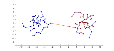
Figure 2: A simple 2-clustering problem and the associated tree and break edge.

The rest of this section is devoted to the post-processing algorithm that tries to reduce the residue number of the subpartition obtained as the output of Algorithm 2. For this it is natural to consider the following decision problem.

MINIMUM RESIDUE NUMBER
INSTANCE: A weighted tree $T=(V,E,\omega,\varphi)$ (without potentials) and two integers $k>1,N\geq 0$. QUERY: Does there exist a minimizing subpartition $\mathcal{A}\in\mathscr{D}_{k}(V)$ achieving ${\rm MISO}_{k}(T)$ whose residue number is at most $N$?

Unfortunately, the following proposition shows that one may just hope for an approximation of the above problem since the decision problem is actually $NP$-complete.

Proposition 4.
The decision problem MINIMUM RESIDUE NUMBER is $NP$-complete in the strong sense for weighted trees.

Proof:

See Appendix for a proof. ∎

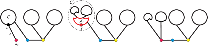
Figure 3: A typical scheme of the post-process subroutine.

In what follows we propose an approximation scheme for the above problem which will constitute the post-process part of the main algorithm (a schematic general case of this procedure is depicted in Figure 3 which can be helpful in following the details that will follow).

In order to ensure a high intra-cluster similarity we try to force the induced subgraph on each cluster to form a connected subgraph. Therefore, our basic strategy is to look for a minimizing subpartition with a small residue number whose parts induce connected subgraphs.

To find such a subpartition, with an initial good subpartition in hand, we follow the following post-processing procedure that checks the two following facts,

1. Each part of the subpartition induces connected subgraphs.

2. No subset of residue elements can be added to any part to make a better subpartition with the same connectivity property.

For this, assume that $\mathcal{A}=\{A_{1},\ldots,A_{k}\}\in\mathscr{D}_{k}(X)$ is the minimizing subpartition, obtained from Algorithm 2. Also, in order to keep the pseudo-code concise we introduce the following terms.

1. Non-residue vertex: A vertex in $\cup_{i=1}^{k}A_{i}$.

2. Break edge: An edge in $E(A_{i},A_{i}^{c})$ for some $i$.

3. Residue subtree: A subtree obtained by removing all break edges from the original tree whose all vertices are residue elements.

4. Start vertex of a residue subtree: A residue element in the residue subtree which is one end of a break edge.

Figure 2 shows a typical pattern of a break edge and the corresponding tree for a simple 2-clustering problem using the above algorithm.

The post-process algorithm can be summarized as follows (see Figure 3).

1. Compute all residue subtrees.

2. Contract each $A_{i}$ with the normalized flow $f_{i}$ to a single vertex $a_{i}$ and set $a_{t}:=a_{i}$ which has the maximum $f_{i}$.

3. Let $C$ be a non-flagged residue subtree connected to $a_{t}$ with start vertex $s$ and break edge $e$.

4. Contract edge $e$ to obtain a new residue subtree $C^{\prime}$ and start vertex $s^{\prime}$ and update the weights.

5. Run Algorithm 3 on $C^{\prime}$ with the root $s^{\prime}$ and $N:={\rm MISO}(T)$ and let $A^{\prime}_{t}$ be the output.

6. If $A^{\prime}_{t}$ is empty, flag $C$ and goto Step 3, otherwise:

   1. replace $A_{t}$ by $A^{\prime}_{t}$.

   2. update the residue subtree $C$.

   3. clear the flags of all residue subtrees.

   4. goto Step 2.

Algorithm 3 Post-process

  Input a subtree C with the root $s$ and rational number $N$.

  Order the vertices of $C$ in BFS order as $x_{1},x_{2},\ldots,x_{t}=s$.

  Set $i=1$ and initialize set function $\eta:V(C)\to\mathcal{P}(V(C))$ by $\eta(x_{i}):=\{x_{i}\}$.

  for $i=1$ to $t$ do

     $u=parent(x_{i})$.

     $e=\{x_{i},u\}$.

     if $p(x_{i})-\varphi(e)\leq N\ \omega(x_{i})$ then

        $p(u)\leftarrow p(u)+p(x_{i})$.

        $\omega(u)\leftarrow\omega(u)+\omega(x_{i})$.

        $\eta(u)\leftarrow\eta(u)\cup\eta(x_{i})$.

     else

        $p(u)\leftarrow p(u)+\varphi(e)$.

     end if

  end for

  return  $\eta(s)$

In order to prove that the procedure performs correctly, we should prove that searching inside each residue subtree is sufficient to ensure the properties mentioned before. For this, assume that $\mathcal{A}=\{A_{1},\ldots,A_{k}\}\in\mathscr{D}_{k}(X)$ is a minimizing subpartition. Let $C_{1}$ and $C_{2}$ be two residue subtrees and for each $i=1,2$, let $S_{i}\subset C_{i}$ be a subset connected to $A_{1}$. Then we have

$$\frac{\varphi(\partial A_{1})+p(A_{1})}{\omega(A_{1})}\leq{\rm MISO}_{k}(T).$$ (4)

Now, if

$$\forall\ i=1,2,\ \frac{\varphi(\partial(A_{1}\cup S_{i}))+p(A_{1}\cup S_{i})}{\omega(A_{1}\cup S_{i})}>{\rm MISO}_{k}(T),$$ (5)

then from (4) and (5), we conclude that

$$\frac{\varphi(\partial(A_{1}\cup S_{1}\cup S_{2}))+p(A_{1}\cup S_{1}\cup S_{2})}{\omega(A_{1}\cup S_{1}\cup S_{2})}>{\rm MISO}_{k}(T).$$

This clearly shows that searching inside each residue subtree for a good subset is sufficient to find all good subsets, and hence, the post-process algorithm performs correctly.

III Analysis and Experimental Comparison

In this section we go through the time complexity and performance analysis of our proposed algorithm.

TABLE I: Performance on UCI database (global scaling): NJW=Ng-Jordan-Weiss [24], LT=Li-Tian [19], GS=Grady-Schwartz [11], SM=Shi-Malik [29], WJHZQ=Wang et. al. [32], DJS=this paper.

					$\sigma=0.09$
Data set	Size	Cluster No.	Dim.	NJW	LT	GS	SM	WJHZQ	DJS
Wine	178	3	13	0.331461	0.286517	0.471910	0.297753	0.325843	0.280899
Iris	150	3	4	0.100000	0.066667	0.333333	0.100000	0.040000	0.040000
Breast	106	6	9	0.632075	0.594340	0.603774	0.698113	0.471698	0.500000
Segmentation	210	7	19	0.561905	0.476190	0.566667	0.371429	0.395238	0.409524
Glass	214	6	10	0.556075	0.457944	0.588785	0.467290	0.658879	0.528037
Average				0.4363	0.3763	0.5129	0.3869	0.3783	0.3573

TABLE II: Performance on UCI database (local scaling): NJW=Ng-Jordan-Weiss [24], LT=Li-Tian [19], GS=Grady-Schwartz [11], SM=Shi-Malik [29], WJHZQ=Wang et. al. [32], DJS=this paper.

					$\nu=30$
Data set	Size	Cluster No.	Dim.	NJW	LT	GS	SM	WJHZQ	DJS
Wine	178	3	13	0.280899	0.280899	0.280899	0.280899	0.308989	0.280899
Iris	150	3	4	0.086667	0.073333	0.333333	0.100000	0.040000	0.040000
Breast	106	6	9	0.622642	0.622642	0.622642	0.641509	0.471698	0.509434
Segmentation	210	7	19	0.404762	0.504762	0.609524	0.404762	0.347619	0.423810
Glass	214	6	10	0.560748	0.495327	0.504673	0.644860	0.658879	0.560748
Average				0.3911	0.3954	0.4702	0.4144	0.3654	0.3574

III-A Time complexity analysis

Based on the details presented in the previous section the algorithm consists of three phases:

• PHASE I: A pre-processing phase where an affinity graph is constructed from the input data and a minimum spanning tree of the graph is obtained.

• PHASE II: A tree-partitioning phase where the minimum spanning tree is sub-partitioned according to an isoperimetry criteria (Algorithm 2).

• PHASE III: A post-processing phase where residue subtrees are reprocessed in order to find a minimizing subpartition with the minimal residue number.

In what follows we elaborate on estimating the time complexity of each phase. We denote the time complexity function of the algorithm with $t(n)$ where $n$ is the size of the data set, where

$$t(n)=t_{1}(n)+t_{2}(n)+t_{3}(n),$$ (6)

in which $t_{i}(n)$ denotes the time complexity of the $i$’th phase. The following analysis will show that $t(n)\in O(n^{2})$ in the worst case for the global scaling scenario with a post-processing, where in the local scaling setting it is observed that the basic algorithm operates in $O(n\log n)$ time.

III-A1 PHASE I

It is supposed that the $i$’th object of interest is given in a vector representation $F_{[d\times 1]}^{i}$ where each element of the feature vector is a real number ($d$ is a fixed integer). Also, it is presumed that a similarity function $S:\mathbb{R}^{d}\times\mathbb{R}^{d}\rightarrow\mathbb{R}$ is given with computational complexity $O(t_{S}(d))=O(c)$ for a constant $c$.

In construction of a global scale affinity graph one needs $\binom{n}{2}\in O(n^{2})$ times computation of the similarity function. On the other hand, in a local scale affinity graph (e.g. see [36]) it is enough to focus on a fixed proximity of each vertex (e.g. as is the case in image segmentation application) and consequently, one may use any technique for nearest neighbour search problem as space partitioning, locality sensitive hashing, approximate nearest neighbour or other well-known methods to obtain the affinity graph of the input vectors in sub-polynomial time. Assuming that the input vectors belong to a space with a Minkowski metric (which is usually the case in real applications) one may use $\epsilon-$approximate nearest neighbour to find a fixed number $\nu$ of neighbours for each object that results in a graph with size $|E|\in O(n)$ which is constructed in time $O(n\log n)$ for a fixed $\epsilon$.

Given a graph of size $|E|\in O(n)$ one may easily find a minimum spanning tree using well-known algorithms in time at most $O(n\log n)$.

Hence, in a local scaling model we may assume that $t_{1}(n)\in O(n\log n)$ and in the global scaling model we have $t_{1}(n)\in O(n^{2})$ in the worst case.

III-A2 PHASE II

Time complexity of Algorithm 1 was shown to be linear in [5]. We verified within the proof of Theorem 1, that the runtime of Algorithm 2 lies in $O(n\log n)$. Thus, with the notations in the proof of Theorem 1, we have

$$t_{2}(n) \in O\left(n\left(\log({2{\omega^{*}}^{2}(\beta_{0}-\alpha_{0}}))-\log({\varphi_{*}+p_{*}})\right)\right)$$

$$=O(n\log n).$$

III-A3 PHASE III

By definitions the worst case time complexity of the post-processing algorithm is bounded by $O(n^{2})$, since one may think of a case where all connected components of the subgraph are of order one. However, it should be noted that in our real experiments the generic cases were observed to be far from the worst case.

III-B Experimental results

In this section we provide our experimental comparison of proposed algorithm with some similar algorithms on some well-known clustering datasets. In our experiments the edge weights are assumed to be equal to

$$\varphi(uv)=\exp(-\frac{S(u,v)}{\sigma})$$ (7)

following the convention in clustering literature, where $\sigma$ is the scaling parameter. Also, hereafter, $\nu$ stands for the neighbourhood parameter for local scaling.

III-B1 UCI benchmarks

Table I reports the outcome of the performance analysis of four algorithms on UCI machine-learning benchmark repository [30]. Each number in the table represents the misclassification rate (i.e. the ratio of incorrect labellings to the total number of objects) for the corresponding algorithm. For the algorithms that do not get the number of clusters as a part of the input a precision threshold is set and the algorithm is terminated after that stage. We should also report that the GS algorithm just terminated on the Iris data set with a $2$-clustering and this is the main reason for this algorithm relatively high misclassification rate in this case.

III-B2 Some hard instances

We have also considered the performance of our algorithm on a couple of hard artificial clustering problems as is depicted in Figure 4. As it is clear from the results the algorithm has been successful enough to extract the correct expected clusters.

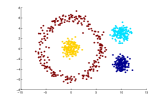
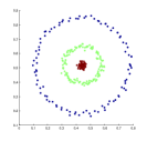
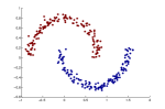
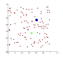
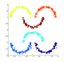
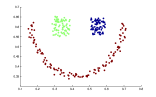
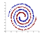
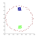
Figure 4: The first column contains a set of hard problems created artificially and the second column consists of four cases chosen from http://www.vision.caltech.edu/lihi/Demos/SelfTuningClustering.html where the local scaling parameter is set to $\nu=7$ ($\sigma=0.1$ for all problems).

IV The outlier profile of a data-set

In this section we try to show how our new extended model can be used to formalize the concept of an outlier set. First of all, it should be noted that the concept of an outlier is not easy to formalize since it certainly depends on the data scaling factors. Although, there has been very little on the formalization of this concept (e.g. see [7] as a very exceptional nice reference), we believe that one should try to define the concept of an outlier profile of a data set (to be made precise later) than trying to define the concept of an outlier set, since depending on ones precision about the concept of being far, one may come to very different conclusions about what an outlier is. Hence, in what follows we use the flexibility of potentials, already introduced in our model, to simulate this precision analysis, and consequently, we will be able to define the concept of an outlier set with respect to a precision parameter $\alpha$. Therefore, using this parametrization one comes to a varying family of sets that will be called the outlier profile of the data set. Using this we will also try to extract the best candidate for an outlier set and we will propose a criteria for extracting such a set while we will also provide an approximation algorithm to approach to a solution for the problem. We also provide experimental results that can serve as evidence to the correctness and applicability of our approach.

We would like to note that this section is just a starter to these ideas and we believe there is a lot more that should be investigated theoretically and experimentally.

Definition 5.
Let $G=(X,E,\omega,\varphi,p)$ be a weighted graph with potential. Then given $k\in\mathbb{N}$ and $\alpha\in\mathbb{R}^{+}$, for any $\mathcal{A}\in\mathscr{D}_{k}(X)$ define

$${\rm cost}_{k,\alpha}(\mathcal{A}):=\max_{1\leq i\leq k}\frac{\varphi(\partial A_{i})+\alpha\ p(A_{i})}{\omega(A_{i})},$$ (8)

and

$${\rm MISO}_{k,\alpha}(G):=\min_{\mathcal{A}\in\mathscr{D}_{k}(X)}{\rm cost}_{k,\alpha}(\mathcal{A}).$$

A subset $A\subset V$ is said to be a $(k,\alpha)$-outlier of $G$ if for any $\beta\geq\alpha$, the subset $A$ does not intersect any minimizer of ${\rm MISO}_{k,\beta}(G)$. It is clear by definition that any subset of a $(k,\alpha)$-outlier of $G$ is also a $(k,\alpha)$-outlier of $G$. Hence, we define the $(k,\alpha)$-outlier set of $G$, $O_{k,\alpha}(G)$, to be the union of all $(k,\alpha)$-outliers of $G$ which is itself a maximal $(k,\alpha)$-outlier of $G$.

Note that the concept of an $(k,\alpha)$-outlier also depends on the potential function $p$. Also, Now, as a direct consequence of definition we have,

Proposition 6.
Given positive real numbers $\alpha\leq\beta$ and a weighted graph $G=(X,E,\omega,\varphi,p)$, then $O_{k,\alpha}(G)\subseteq O_{k,\beta}(G).$

In order to match the definition with our intuition about outlier sets we should relate the potential function to the distance (i.e. the inverse of the similarity) function, and for this we adopt the special potential function for which the potential at each vertex is the mean of the distance of the vertex to the rest of the vertices.

$$p(x):=\frac{1}{n}\sum_{y\in X}\|x-y\|_{{}_{2}}.$$

To get a feeling about how this definition works one may refer to the artificial example depicted in Figure 6 in which one can see that the residue of the minimizing subpartition increases as a consequence of an increase in the potential function (i.e. an increase of $\alpha$).

Now, the main problem is how one may approximately compute the outlier profile of a best candidate for an outlier set based on the above mentioned definition. For this, consider Figure 5 that shows the way of increasing of the residue number as increasing of $\alpha$ for the graph of Figure 6. Hereafter, this function is called the outlier profile of the graph.

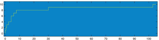
Figure 5: An approximation of the outlier profile of the graph depicted in Figure 6.

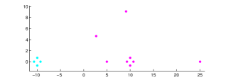
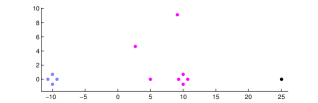
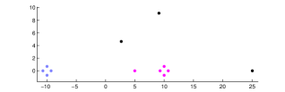
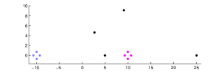
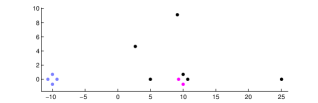
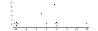
Figure 6: The increase of residues as $\alpha$ increases (residue vertices are depicted in black for $\alpha=0,0.6,0.8,2,5,50$).

Now, our main problem is to extract the best candidate for an outlier set. For this, one may note that a possible natural criteria for this is a relatively long delay in a constant value in the outlier profile which is also close to the origin. As it is clear, the two intuitive conditions namely, being close to the origin (i.e. small $\alpha$) and having a long stay in a constant value, are contradictory to each other and to set a criterion one needs an scaling factor. Hence we let the parameter $\sigma_{s}$ to be the desired scaling factor and define

$$sm(I_{i})=\exp(\frac{-\min(I_{i})}{\sigma_{s}})-\exp(\frac{-(\max(I_{i})}{\sigma_{s}}),$$ (9)

in which $I_{i}=[\min(I_{i}),\max(I_{i})]$ is the $i$’th interval on which the number of residues remains constant. Hence, we let the interval $I_{*}$ be the interval on which $sm(I_{i})$ is maximized and choose this interval as the space in which the best $\alpha$ lives. Following this idea we define

$$\alpha_{*}=\min(I_{*}).$$ (10)

Algorithm 4 HeuristicSearch

0:  BPs($1...n-k$) = [$\infty,-\infty$] , $a<b$, $n_{a}<n_{b}$

  Input $BPs,[a,b],[n_{a},n_{b}],T,P,\epsilon$

  if $b-a\leq\epsilon$ then

     return  BPs

  else

     $\alpha=\frac{a+b}{2}$

     subpartition = {The output of Algorithm 2}

     $resno$ =ResidueNumber(subpartition)

     if $resno\leq n_{a}$  then

        Update all BPs from index $resno+1$ to $n_{a}$

        BPs = HeuristicSearch($BPs,[\alpha,b],[resno,n_{b}],T,P,\epsilon$)

     else if resno $\geq n_{b}$ then

        Update all BPs from index $n_{b}+1$ to $resno$

        BPs = HeuristicSearch($BPs,[a,\alpha],[n_{a},n_{b}],T,P,\epsilon$)

     else

        Update BPs with index resno

        if resno $>n_{a}$ then

           BPs = HeuristicSearch($BPs,[a,\alpha],[n_{a},resno],T,P,\epsilon$)

        end if

        if resno $<n_{b}$ then

           BPs = HeuristicSearch($BPs,[\alpha,b],[resno,n_{b}],T,P,\epsilon$)

        end if

     end if

  end if

Since it is a hard problem to extract the whole outlier profile of a graph, we use our clustering algorithm to find an approximate minimizer for each $\alpha$ and we also apply a binary search on the spectrum of $\alpha$ to extract $I_{*}$ and $\alpha_{*}$ up to a predefined precision. Such an approximation algorithm is described in Algorithm 4. It is important to note that based on what follows we can deduce that the performance of our algorithm is acceptable despite approximation, however the effect of approximation on the final result are undeniable (e.g. see Figure 9). Also, it should be noted that making the precision factors finer (e.g. smaller steps in the binary search) will give rise to a longer runtime which is undesirable.

In order to evaluate the performance of the proposed algorithm we consider a couple of artificial problems. At first we applied the algorithm to the artificial clustering problems in Figure 7. As it is clear from the results, the algorithm has been able to correctly extract clusters as well as the outlier set.

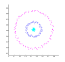
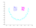
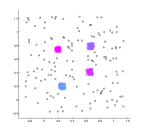
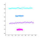
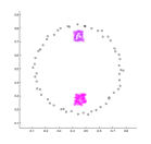
Figure 7: Performance of Algorithm 4 (black spots are extracted outlier data points and $\sigma_{s}$ = 0.1 for all problems).

In our final experimental evaluation we focus on the performance of the algorithm of Wang et. al. [32] since it has the best performance according to our analysis in Section III and also since using a proper local scaling parameter it is capable of extracting the outlier set as a cluster. In this direction we first consider a hard artificial clustering problem with outliers as depicted in Figure 8. As it is clear from the results our algorithm has been able to successfully extract the outliers.

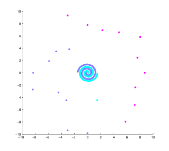
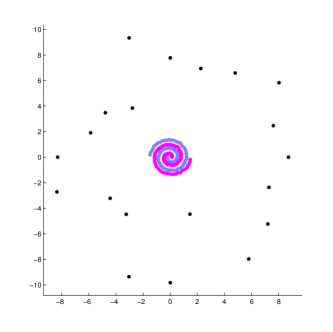
Figure 8: A problem with global affinity $\sigma=0.09$ and $\sigma_{s}=0.5$. First row contains the outcome of WJHZQ [32] Algorithm. Second row contains the outcome of our algorithm with $\alpha_{*}=0.25$.

On the other hand, in order to test the impact of the local scaling on the performance we also consider a hard artificial clustering problem as depicted in Figure 9 and as it is clear there are scaling parameters for which we can successfully extract the outlier set. In this regard it should be noted that in the local scaling setting for each individual case one can always find scaling parameters that works well, however, in our approach one may use the algorithm with as large a local scaling parameter as possible (considering ones runtime limits) without being concerned about the effect of this parameter on the performance of outlier extraction, while in the rest of the algorithms it is essentially this parameter which somehow tunes the algorithm to extract the outlier set as a cluster which is not consistent when one is dealing with a variety of different data sets.

Figure 9: A problem with local affinity parameter $\nu=20$ and $\sigma_{s}=0.5$ . First row contains the outcome of WJHZQ [32] Algorithm. Second row contains the outcome of our algorithm with $\alpha_{*}=0.24$.

[Proof of Proposition 2] Consider the following problem which is well-known to be $NP$-complete in the strong sense [9].

3-PARTITION
INSTANCE: A positive integer $B$ and $3m$ positive integers $w_{1},\ldots,w_{3m}$, such that $B/4<w_{i}<B/2$, for each $1\leq i\leq 3m$ and $\sum_{i=1}^{3m}w_{i}=mB$. QUERY: Is there an $m$-partition $\{S_{i}\}^{m}_{1}\in{\mathcal{P}}_{m}([3m])$ such that, for each $1\leq j\leq m$, $\sum_{i\in S_{j}}x_{i}=B$?

We provide a reduction from the 3-PARTITION problem. Assume that the integers $w_{1},\ldots,w_{3m}$ together with the integer $B$ is an instance of the problem 3-PARTITION. Let $t$ be a fixed positive integer and construct the weighted tree $T=(V,E,\omega,\varphi)$ as follows.

$$V :=\{x,x_{i},y_{j},z_{l}\ |\ 1\leq i\leq 3m,1\leq j\leq m,1\leq l\leq t\},$$

$$E :=\{xx_{i},xy_{j},xz_{l}\ |\ 1\leq i\leq 3m,1\leq j\leq m,1\leq l\leq t\}.$$

Vertex weights are defined as follows.

$$\omega(x):=1, \ \omega(x_{i}):=w_{i}+B+1,\ \forall\ 1\leq i\leq 3m,$$

$$\ \omega(y_{j}):=1,\ \forall\ 1\leq j\leq m,$$

$$\ \omega(z_{l}):=B+1,\ \forall\ 1\leq l\leq t.$$

All edge weights is set to be equal to $1$. Let $k=m+t$ and $N=1$ to get an instance of the problem MINIMUM RESIDUE NUMBER. We assume that $t$ is sufficiently large (e.g. $t>7m$). We are going to show that ${\rm MISO}_{k}(T)={1}/{(B+1)}$. First note that for the subpartition $\mathcal{A}:=\{\{x_{1}\},\ldots,\{x_{3m}\},\{z_{1}\},\ldots,\{z_{t}\}\}$, we have ${\rm cost}(\mathcal{A})={1}/{(B+1)}$ and thus ${\rm MISO}_{k}(T)\leq 1/(B+1)$. On the other hand, let $\mathcal{B}:=\{B_{1},\ldots,B_{k}\}$ be a minimizing subpartition achieving ${\rm MISO}_{k}(T)$. Then there is some $B_{i}$ which is completely included in the set $\{z_{1},\ldots,z_{t}\}$. Thus ${\rm cost}(\mathcal{B})\geq 1/(B+1)$. This shows that ${\rm MISO}_{k}(T)=1/(B+1)$.

Now assume that the answer to 3-PARTITION is positive and let $\{S_{1},\ldots,S_{m}\}$ be a partition of $[3m]$, where the sum of the elements of each $S_{i}$ is equal to $m$. Therefore each $S_{i}$ has exactly 3 elements. Now define the $k-$subpartition $\mathcal{A}:=\{A_{1},\ldots,A_{k}\}$ as follows,

$$A_{j} :=\{y_{j},x_{i}\ |\ i\in S_{j}\},\ \forall\ 1\leq j\leq m,$$

$$A_{j} :=\{z_{j-m}\},\ \forall\ m+1\leq j\leq t+m.$$

We have $\mathcal{A}$ is a minimizing subpartition achieving ${\rm MISO}_{k}(T)=1/(B+1)$ whose residue number is $1$.

Now, conversely, assume that there exists a minimizing subpartition $\mathcal{B}$ achieving ${\rm MISO}_{k}(T)=1/(B+1)$ whose residue number is at most $1$. Then the vertex $x$ is a residue element for $\mathcal{B}$. Because for each $i$, $|B_{i}|\leq 3m+2$ and if $x\in B_{1}$, then ${\rm cost}(\mathcal{B})\geq t/2(3m+1)(B+1)>1/(B+1)$. Hence $\mathcal{B}$ is a partition of the set $V\setminus\{x\}$. Since ${\rm cost}(\mathcal{B})=1/(B+1)$, for all $1\leq i\leq k$, the average of the weights of vertices in $B_{i}$ is at least $B+1$. Now delete all vertices $z_{1},\ldots,z_{t}$ from $B_{i}$’s to obtain $m$ nonempty subsets $B^{\prime}_{1},\ldots,B^{\prime}_{m}$ with the average weights of at least $B+1$. Since the average weight of all vertices $\{x_{i},y_{j}\ |\ 1\leq i\leq 3m,1\leq j\leq m\}$ is $B+1$, the average weight of each $B^{\prime}_{i}$ is exactly $B+1$. Now, since $w_{i}$’s are positive, each $B^{\prime}_{i}$ contains exactly one of the vertices $y_{1},\ldots,y_{m}$. Hence for each $1\leq i\leq m$, $\sum_{x_{p}\in B^{\prime}_{i}}w_{p}=B$. This finishes the reduction.

References

- [1] S. Arora, S. Rao, and U. Vazirani, “Expander flows, geometric embeddings and graph partitioning,” in Proceedings of the thirty-sixth annual ACM symposium on theory of computing, ser. STOC ’04. New York, NY, USA: ACM, 2004, pp. 222–231.
- [2] T. Asano, B. Bhattacharya, M. Keil, and F. Yao, “Clustering algorithms based on minimum and maximum spanning trees,” in Proceedings of the fourth annual symposium on computational geometry, ser. SCG ’88. New York, NY, USA: ACM, 1988, pp. 252–257.
- [3] Y. Bengio, O. Delalleau, N. Le Roux, J. . Paiement, P. Vincent, and M. Ouimet, “Learning eigenfunctions links spectral embedding and kernel pca,” Neural computation, vol. 16, no. 10, pp. 2197–2219, 2004.
- [4] A. Daneshgar, H. Hajiabolhassan, and R. Javadi, “On the isoperimetric spectrum of graphs and its approximations,” J. Comb. Theory Ser. B, vol. 100, pp. 390–412, July 2010.
- [5] A. Daneshgar and R. Javadi, “On the complexity of isoperimetric problems on trees,” Discrete Applied Mathematics, vol. 160, pp. 116–131, 2012.
- [6] E. D. Demaine, D. Emanuel, A. Fiat, and N. Immorlica, “Correlation clustering in general weighted graphs,” Theoretical Computer Science, vol. 361, no. 2-3, pp. 172–187, 2006.
- [7] J. Dunagan and S. Vempala, “Optimal outlier removal in high-dimensional spaces,” J. Comput. Syst. Sci., vol. 68, no. 2, pp. 335–373, 2004.
- [8] G. W. Flake, R. E. Tarjan, and K. Tsioutsiouliklis, “Graph clustering and minimum cut trees,” Internet Mathematics, vol. 1, no. 4, pp. 385–408, 2004.
- [9] M. R. Garey and D. S. Johnson, Computers and intractability, A guide to the theory of NP-completeness. San Francisco, Calif.: W. H. Freeman and Co., 1979.
- [10] L. Grady, “Fast, quality, segmentation of large volumes - isoperimetric distance trees,” in ECCV (3), 2006, pp. 449–462.
- [11] L. Grady and E. L. Schwartz, “Isoperimetric graph partitioning for image segmentation,” IEEE Trans. Pattern Anal. Mach. Intell., vol. 28, pp. 469–475, March 2006.
- [12] O. Grygorash, Y. Zhou, and Z. Jorgensen, “Minimum spanning tree based clustering algorithms,” in Proceedings of the 18th IEEE International Conference on Tools with Artificial Intelligence, ser. ICTAI ’06. Washington, DC, USA: IEEE Computer Society, 2006, pp. 73–81.
- [13] F. P. Jain A.K., Murty M.N., “Data clustering: a review,” ACM Computing Surveys, vol. 31, pp. 264–323, 1999.
- [14] R. Javadi, “Isoperimetric problems on graphs,” Ph.D. dissertation, Sharif University of Technology, Tehran, 2011.
- [15] D. S. Johnson, “The NP-completeness column: an ongoing guide,” Journal of Algorithms, vol. 6, pp. 434–451, 1985.
- [16] R. Kannan, S. Vempala, “Spectral algorithms,” Found. Trends Theor. Comput. Sci., vol. 4, no. 3-4, pp. front matter, 157–288 (2009), 2008.
- [17] R. Kannan, S. Vempala, and A. Vetta, “On clusterings: good, bad and spectral,” Journal of the ACM, vol. 51, pp. 497–515, May 2004.
- [18] M. Laszlo and S. Mukherjee, “Minimum spanning tree partitioning algorithm for microaggregation,” IEEE Transactions on Knowledge and Data Engineering, vol. 17, pp. 902–911, 2005.
- [19] X. Li and Z. Tian, “Optimum cut-based clustering,” Signal Process., vol. 87, pp. 2491–2502, November 2007.
- [20] A. Louis, P. Raghavendra, P. Tetali, and S. Vempala, Algorithmic extensions of Cheeger’s inequality to higher eigenvalues and partitions, ser. Lecture Notes in Computer Science (including subseries Lecture Notes in Artificial Intelligence and Lecture Notes in Bioinformatics), 2011, vol. 6845 LNCS.
- [21] U. Von Luxburg, “A tutorial on spectral clustering,” Statistics and Computing, vol. 17, no. 4, pp. 395–416, 2007.
- [22] U. Von Luxburg, M. Belkin, and O. Bousquet, “Consistency of spectral clustering,” Ann. Statist., vol. 36, no. 2, pp. 555–586, 2008.
- [23] B. Mohar, “Isoperimetric numbers of graphs,” Journal of Combinatorial Theory, Series B, vol. 47, no. 3, pp. 274 – 291, 1989.
- [24] A. Y. Ng, M. I. Jordan, and Y. Weiss, “On spectral clustering: analysis and an algorithm,” in Advances in Neural Information Processing Systems. MIT Press, 2001, pp. 849–856.
- [25] N. Päivinen, “Clustering with a minimum spanning tree of scale-free-like structure,” Pattern Recognition Letters, vol. 26, no. 7, pp. 921–930, 2005.
- [26] Y. W. J. Peng, “Approximating k-means-type clustering via semidefinite programming,” SIAM Journal on Optimization, vol. 18, no. 1, pp. 186–205, 2007.
- [27] O. S. Rothaus, “Analytic inequalities, isoperimetric inequalities and logarithmic Sobolev inequalities,” J. Funct. Anal., vol. 64, no. 2, pp. 296–313, 1985.
- [28] S. E. Schaeffer, “Graph clustering,” Computer Science Review, vol. 1, no. 1, pp. 27–64, 2007.
- [29] J. Shi and J. Malik, “Normalized cuts and image segmentation,” IEEE Trans. Pattern Anal. Mach. Intell., vol. 22, pp. 888–905, August 2000.
- [30] “UCI machine learning repository,” http://archive.ics.uci.edu/ml/.
- [31] S. S. Vempala, Spectral algorithms for learning and clustering, ser. Lecture Notes in Computer Science (including subseries Lecture Notes in Artificial Intelligence and Lecture Notes in Bioinformatics), 2007, vol. 4539 LNAI.
- [32] J. Wang, Y. Jia, X. . Hua, C. Zhang, and L. Quan, “Normalized tree partitioning for image segmentation,” in 26th IEEE Conference on Computer Vision and Pattern Recognition, CVPR, 2008, pp. 1–8.
- [33] Y. Weiss, “Segmentation using eigenvectors: a unifying view,” in Proceedings of the IEEE International Conference on Computer Vision, vol. 2, 1999, pp. 975–982.
- [34] Y. Xu and E. C. Uberbacher, “2d image segmentation using minimum spanning trees,” Image and Vision Computing, vol. 15, no. 1, pp. 47 – 57, 1997.
- [35] S. X. Yu and J. Shi, “Multiclass spectral clustering,” in Proceedings of the Ninth IEEE International Conference on Computer Vision - Volume 1, ser. ICCV ’03. Washington, DC, USA: IEEE Computer Society, 2003, pp. 313–319.
- [36] L. Zelnik-manor and P. Perona, “Self-tuning spectral clustering,” in Advances in Neural Information Processing Systems 17. MIT Press, 2004, pp. 1601–1608.