Linear MMSE-Optimal Turbo Equalization Using Context Trees

Nargiz Kalantarova, Kyeongyeon Kim, Suleyman S. Kozat, Senior Member, IEEE, and Andrew C. Singer, Fellow, IEEE Andrew C. Singer (acsinger@illinois.edu) is with the Electrical and Computer Engineering Department at University of Illinois at Urbana-Champaign. Suleyman S. Kozat and Nargiz Kalantarova ({skozat,nkalantarova}@ku.edu.tr) are with the Electrical Engineering Department at Koc University, Istanbul, tel: +902123381684, +902123381490. Kim Kyeongyeon (adrianakky@gmail.com) is with Samsung Electronics, Gyeonggi-do, Republic of Korea.
Abstract

Formulations of the turbo equalization approach to iterative equalization and decoding vary greatly when channel knowledge is either partially or completely unknown. Maximum aposteriori probability (MAP) and minimum mean square error (MMSE) approaches leverage channel knowledge to make explicit use of soft information (priors over the transmitted data bits) in a manner that is distinctly nonlinear, appearing either in a trellis formulation (MAP) or inside an inverted matrix (MMSE). To date, nearly all adaptive turbo equalization methods either estimate the channel or use a direct adaptation equalizer in which estimates of the transmitted data are formed from an expressly linear function of the received data and soft information, with this latter formulation being most common. We study a class of direct adaptation turbo equalizers that are both adaptive and nonlinear functions of the soft information from the decoder. We introduce piecewise linear models based on context trees that can adaptively approximate the nonlinear dependence of the equalizer on the soft information such that it can choose both the partition regions as well as the locally linear equalizer coefficients in each region independently, with computational complexity that remains of the order of a traditional direct adaptive linear equalizer. This approach is guaranteed to asymptotically achieve the performance of the best piecewise linear equalizer and we quantify the MSE performance of the resulting algorithm and the convergence of its MSE to that of the linear minimum MSE estimator as the depth of the context tree and the data length increase.

Index Terms:
Turbo equalization, piecewise linear, nonlinear equalization, context tree, decision feedback.

EDICS Category: MLR-APPL, MLR-SLER, ASP-APPL.

I Introduction

Iterative equalization and decoding methods, or so-called turbo equalization [1, 2, 3], have become increasingly popular methods for leveraging the power of forward error correction to enhance the performance of digital communication systems in which intersymbol interference or multiple access interference are present. Given full channel knowledge, maximum aposteriori probability (MAP) equalization and decoding give rise to an elegant manner in which the equlization and decoding problems can be (approximately) jointly resolved [1]. For large signal constellations or when the channel has a large delay spread resulting in substantial intersymbol interference, this approach becomes computationally prohibitive and lower complexity linear equalization strategies are often employed [4, 5, 6]. Computational complexity issues are also exacerbated by the use of multi-input/multi-output (MIMO) transmission strategies. It is important to note that MAP and MMSE formulations of the equalization component in such iterative receivers make explicit use of soft information from the decoder that is a nonlinear function of both the channel response and the soft information [5]. In a MAP receiver, soft information is used to weight branch metrics in the receiver trellis [7]. In an MMSE receiver, this soft information is used in the (recursive) computation of the filter coefficients and appears inside of a matrix that is inverted [5].

In practice, most communication systems lack precise channel knowledge and must make use of pilots or other means to estimate and track the channel if the MAP or MMSE formulations of turbo equalization are to be used [7, 5]. Increasingly, however, receivers based on direct adaptation methods are used for the equalization component, due to their attractive computational complexity [4, 8, 9]. Specifically, the channel response is neither needed nor estimated for direct adaptation equalizers, since the transmitted data symbols are directly estimated based on the signals received. This is often accomplished with a linear or decision feedback structure that has linear complexity in the channel memory, as opposed to the quadratic complexity of the MMSE formulation, and is invariant to the constellation size [8]. A MAP receiver not only needs a channel estimate, but also has complexity that is exponential in the channel memory, where the base of the exponent is the transmit constellation size [7]. For example, underwater acoustic communications links often have a delay spread in excess of several tens to hundreds of symbol periods, make use of 4 or 16 QAM signal constellations, and have multiple transmitters and receive hydrophones [9, 10]. In our experience, for such underwater acoustic channels, MAP-based turbo equalization is infeasible and MMSE-based methods are impractical for all but the most benign channel conditions [9]. As such, direct-adaptation receivers that form an estimate of the transmitted symbols as a linear function of the received data, past decided symbols, and soft information from the decoder have emerged as the most pragmatic solution. Least-mean square (LMS)-based receivers are used in practice to estimate and track the filter coefficients in these soft-input/soft-output decision feedback equalizer structures, which are often multi-channel receivers for both SIMO and MIMO transmissions [8, 4, 6].

While such linear complexity receivers have addressed the computational complexity issues that make MAP and MMSE formulations unattractive or infeasible, they have also unduly restricted the potential benefit of incorporating soft information into the equalizer. Although such adaptive linear methods may converge to their “optimal”, i.e., Wiener solution, they usually deliver inferior performance compared to a linear MMSE turbo receiver[11], since the Wiener solution for this stationarized problem, replaces the time-varying soft information by its time average [5, 12]. It is inherent in the structure of such adaptive approaches that an implicit assumption is made that the random process governing the received data and that of the soft-information sequence are both mean ergodic so that ensemble averages associated with the signal and soft information can be estimated with time averages. The primary source of performance loss of these adaptive algorithms is due to their implicit use of the log likelihood ratio (LLR) information from the decoder as stationary soft decision sequence [11], whereas a linear MMSE turbo equalizer considers this LLR information as nonstationary a priori statistics over the transmitted symbols [5].

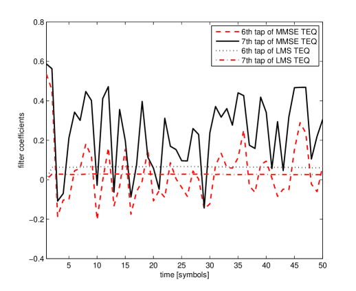
Indeed, one of the strengths of the linear MMSE turbo equalizer lies in its ability to employ a distinctly different linear equalizer for each transmitted symbol [5, 6]. This arises from the time-varying nature of the local soft information available to the receiver from the decoder. Hence, even if the channel response were known and fixed (i.e., time-invariant), the MMSE-optimal linear turbo equlizer correponds to a set of linear filter coefficients that are different for each and every transmitted symbol [13],[5]. This is due to the presence of the soft information inside a inverted matrix that is used to construct the MMSE-optimal equalizer coefficients. As a result, a time-invariant channel will still give rise to a recursive formulation of the equalizer coefficients that require quadratic complexity per output symbol. As an example in Fig. 1, we plot for a time invariant channel the time varying filter coefficients of the MMSE linear turbo equalizer, along with the filter coefficients of an LMS-based, direct adaptation turbo equalizer that has converged to its time invariant solution. This behavior is actually manifested due to the nonlinear relationship between the soft information and the MMSE filter coefficients.
Refer to caption

Figure 1: An example of time varying filter coefficients of an MMSE turbo equalizer (TEQ) and steady state filter coefficients of an LMS turbo equalizer (TEQ) in a time invariant ISI channel [0.227,0.46,0.688,0.46,0.227]0.2270.460.6880.460.227[0.227,0.46,0.688,0.46,0.227] at the second turbo iteration. (SNR=10dB𝑆𝑁𝑅10𝑑𝐵SNR=10dB, feedforward filter length =151515, step size = 0.0010.0010.001, BPSK, random interleaver and 1212\frac{1}{2} rate convolutional code with constraint length of 333 are used)

In this paper, we explore a class of equalizers that maintain the linear complexity adaptation of linear, direct adaptation equalizers [8], but attempt to circumvent the loss of this nonlinear dependence of the MMSE optimal equalizer on the soft information from the decoder [5]. Specifically, we investigate an adaptive, piecewise linear model based on context trees [14] that partition the space of soft information from the decoder, such that locally linear (in soft information space) models may be used. However instead of using a fixed piecewise linear equalizer, the nonlinear algorithm we introduce can adaptively choose the partitioning of the space of soft information as well as the locally linear equalizer coefficients in each region with computational complexity that remains on the order of a traditional adaptive linear equalizer [7]. The resulting algorithm can therefore successfully navigate the short-data record regime, by placing more emphasis on lower-order models, while achieving the ultimate precision of higher order models as the data record grows to accommodate them. The introduced equalizer can be shown to asymptotically (and uniformly) achieve the performance of the best piecewise linear equalizer that could have been constructed, given full knowledge of the channel and the received data sequence in advance. Furthermore, the mean square error (MSE) of this equalizer is shown to convergence to that of the minimum MSE (MMSE) estimator (which is a nonlinear function of the soft information) as the depth of the context tree and data length increase.

Context trees and context tree weighting are extensively used in data compression [14], coding and data prediction [15, 16, 17]. In the context of source coding and universal probability assignment, the context tree weighting method is mainly used to calculate a weighted mixture of probabilities generated by the piecewise Markov models represented on the tree [14]. In nonlinear prediction, context trees are used to represent piecewise linear models by partitioning the space of past regressors [15, 17], specifically for labeling the past observations. Note that although we use the notion of context trees for nonlinear modeling as in [14, 16, 17, 18, 19], our results and usage of context trees differ from [14, 16, 17, 18] in a number of important ways. The “context” used in our context trees correspond to a spatial parsing of the soft information space, rather than the temporal parsing as studied in [14, 16, 17]. In addition, the context trees used here are specifically used to represent the nonlinear dependency of equalizer coefficients on the soft information. In this sense, as an example, the time adaptation is mainly (in addition to learning) due to the time variation of the soft information coming from the decoder, unlike the time dependent learning in [18]. Hence, in here, we explicitly calculate the MSE performance and quantify the difference between the MSE of the context tree algorithm and the MSE of the linear MMSE equalizer, which is the main objective.

The paper is organized as follows. In Section II, we introduce the basic system description and provide the objective of the paper. The nonlinear equalizers studied are introduced in Section III. In Section III, we first introduce a partitioned linear turbo equalization algorithm, where the partitioning of the regions is fixed. We continue in Section III-B with the turbo equalization framework using context trees, where the corresponding algorithm with the guaranteed performance bounds is introduced. Furthermore, we provide the MSE performance of all the algorithms introduced and compare them to the MSE performance of the linear MMSE equalizer. The paper concludes with numerical examples demonstrating the performance gains and the learning mechanism of the algorithm.

II System Description

Throughout the paper, all vectors are column vectors and represented by boldface lowercase letters. Matrices are represented by boldface uppercase letters. Given a vector 𝒙𝒙{x}, 𝒙=𝒙H𝒙norm𝒙superscript𝒙𝐻𝒙\|\mbox{$\mbox{\boldmath${x}$}$}\|=\sqrt{\mbox{$\mbox{\boldmath${x}$}$}^{H}\mbox{$\mbox{\boldmath${x}$}$}} is the l2subscript𝑙2l_{2}-norm, where 𝒙Hsuperscript𝒙𝐻\mbox{$\mbox{\boldmath${x}$}$}^{H} is the conjugate transpose, 𝒙Tsuperscript𝒙𝑇\mbox{$\mbox{\boldmath${x}$}$}^{T} is the ordinary transpose and 𝒙superscript𝒙\mbox{$\mbox{\boldmath${x}$}$}^{*} is the complex conjugate. For a random variable x𝑥x (or a vector 𝒙𝒙{x}), E[x]=x¯𝐸delimited-[]𝑥¯𝑥E[x]=\bar{x} (or E[𝒙]=𝒙¯𝐸delimited-[]𝒙¯𝒙E[\mbox{$\mbox{\boldmath${x}$}$}]=\bar{\mbox{$\mbox{\boldmath${x}$}$}}) is the expectation. For a vector 𝒙𝒙{x}, diag(𝒙)diag𝒙\mathrm{diag}(\mbox{$\mbox{\boldmath${x}$}$}) is a diagonal matrix constructed from the entries of 𝒙𝒙{x} and x(i)𝑥𝑖x(i) is the i𝑖ith entry of the vector. For a square matrix 𝑴𝑴{M}, tr(𝑴)tr𝑴\mathrm{tr}(\mbox{\boldmath${M}$}) is the trace. The sequences are represented using curly brackets, e.g., {x(t)}𝑥𝑡\{x(t)\}. i=1NAisuperscriptsubscript𝑖1𝑁subscript𝐴𝑖\bigcup_{i=1}^{N}A_{i} denotes the union of the sets Aisubscript𝐴𝑖A_{i}, where i=1,,N𝑖1𝑁i=1,\ldots,N. The vec(.)\mathrm{vec}(.) operator stacks columns of a matrix of dimension m×n𝑚𝑛m\times n into a mn×1𝑚𝑛1mn\times 1 column vector [20].

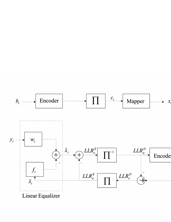
The block diagram of the system we consider with a linear turbo equalizer is shown in Fig. 2. The information bits {b(t)}𝑏𝑡\{b(t)\} are first encoded using an error correcting code (ECC) and then interleaved to generate {c(t)}𝑐𝑡\{c(t)\}. The interleaved code bits {c(t)}𝑐𝑡\{c(t)\} are transmitted after symbol mapping, e.g., x(t)=(1)c(t)𝑥𝑡superscript1𝑐𝑡x(t)=(-1)^{c(t)} for BPSK signaling, through a baseband discrete-time channel with a finite-length impulse response {h(t)}𝑡\{h(t)\}, t=0,1,,M1𝑡01𝑀1t=0,1,\ldots,M-1, represented by 𝒉=[h(M1),,h(0)]Tsuperscript𝒉superscript𝑀10𝑇\mbox{\boldmath${h}$}\stackrel{{\scriptstyle\bigtriangleup}}{{=}}[h(M-1),\ldots,h(0)]^{T}. The communication channel 𝒉𝒉{h} is unknown. The transmitted signal {x(t)}𝑥𝑡\{x(t)\} is assumed to be uncorrelated due to the interleaver. The received signal y(t)𝑦𝑡y(t) is given by

y(t)=k=0M1h(k)x(tk)+n(t),superscript𝑦𝑡superscriptsubscript𝑘0𝑀1𝑘𝑥𝑡𝑘𝑛𝑡y(t)\stackrel{{\scriptstyle\bigtriangleup}}{{=}}\sum_{k=0}^{M-1}h(k)x(t-k)+n(t),

where {n(t)}𝑛𝑡\{n(t)\} is the additive complex white Gaussian noise with zero mean and circular symmetric variance σn2superscriptsubscript𝜎𝑛2\sigma_{n}^{2}. If a linear equalizer is used to reduce the ISI, then the estimate of the desired data x(t)𝑥𝑡x(t) using the received data y(t)𝑦𝑡y(t) is given by

x^(t)=𝒘T(t)[𝒚(t)𝒚¯(t)]+x¯(t),^𝑥𝑡superscript𝒘𝑇𝑡delimited-[]𝒚𝑡¯𝒚𝑡¯𝑥𝑡\hat{x}(t)=\mbox{\boldmath${w}$}^{T}(t)[\mbox{\boldmath${y}$}(t)-\mbox{$\bar{\mbox{\boldmath${y}$}}$}(t)]+\mbox{$\bar{x}$}(t),

where 𝒘(t)=[w(t,N2),,w(t,N1)]T𝒘𝑡superscript𝑤𝑡subscript𝑁2𝑤𝑡subscript𝑁1𝑇\mbox{\boldmath${w}$}(t)=[w(t,N_{2}),\ldots,w(t,-N_{1})]^{T} is length N=N1+N2+1𝑁subscript𝑁1subscript𝑁21N=N_{1}+N_{2}+1 linear equalizer, 𝒚(t)=[y(tN2),,y(t+N1)]Tsuperscript𝒚𝑡superscript𝑦𝑡subscript𝑁2𝑦𝑡subscript𝑁1𝑇\mbox{$\mbox{\boldmath${y}$}$}(t)\stackrel{{\scriptstyle\bigtriangleup}}{{=}}[y(t-N_{2}),\ldots,y(t+N_{1})]^{T} and note that we use negative indices with a slight abuse of notation. The received data vector 𝒚(t)𝒚𝑡\mbox{$\mbox{\boldmath${y}$}$}(t) is given by 𝒚(t)=𝑯𝒙(t)+𝒏(t)𝒚𝑡𝑯𝒙𝑡𝒏𝑡\mbox{$\mbox{\boldmath${y}$}$}(t)=\mbox{\boldmath${H}$}\mbox{$\mbox{\boldmath${x}$}$}(t)+\mbox{$\mbox{\boldmath${n}$}$}(t), where 𝒙(t)=[x(tMN2+1),,x(t+N1)]Tsuperscript𝒙𝑡superscript𝑥𝑡𝑀subscript𝑁21𝑥𝑡subscript𝑁1𝑇\mbox{$\mbox{\boldmath${x}$}$}(t)\stackrel{{\scriptstyle\bigtriangleup}}{{=}}[x(t-M-N_{2}+1),\ldots,x(t+N_{1})]^{T} and 𝑯N×(N+M1)𝑯superscript𝑁𝑁𝑀1\mbox{\boldmath${H}$}\in\mathbbm{C}^{N\times(N+M-1)}

𝑯=[h(M1)h(M2)h(0)000h(M1)h(M2)h(0)0000h(M1)h(M2)h(0)]superscript𝑯delimited-[]𝑀1𝑀200missing-subexpression00𝑀1𝑀20000missing-subexpression0𝑀1𝑀20\mbox{\boldmath${H}$}\stackrel{{\scriptstyle\bigtriangleup}}{{=}}\left[\begin{array}[]{cccccccc}h(M-1)&h(M-2)&\ldots&h(0)&0&\ldots&&0\\ 0&h(M-1)&h(M-2)&\ldots&h(0)&0&\ldots&0\\ \ddots&\ddots&\ddots&\ddots&\ddots&\ddots&\ddots&\ddots\\ 0&\ldots&&0&h(M-1)&h(M-2)&\ldots&h(0)\end{array}\right]

is the convolution matrix corresponding to 𝒉=[h(M1),,h(0)]T𝒉superscript𝑀10𝑇\mbox{\boldmath${h}$}=[h(M-1),\ldots,h(0)]^{T}, the estimate of x(t)𝑥𝑡x(t) can be written as

x^(t)=𝒘T(t)[𝒚(t)𝑯𝒙¯(t)]+x¯(t),^𝑥𝑡superscript𝒘𝑇𝑡delimited-[]𝒚𝑡𝑯𝒙¯𝑡¯𝑥𝑡\hat{x}(t)=\mbox{\boldmath${w}$}^{T}(t)[\mbox{$\mbox{\boldmath${y}$}$}(t)-\mbox{\boldmath${H}$}\mbox{$\bar{\mbox{\boldmath${x}$}}$}(t)]+\mbox{$\bar{x}$}(t), (1)

given that the mean of the transmitted data is known.
Refer to caption

Figure 2: Block diagram for a bit interleaved coded modulation transmitter and receiver with a linear turbo equalizer.

However, in turbo equalization, instead of only using an equalizer, the equalizer and decoder are jointly performed iteratively at the receiver of Fig. 2. The equalizer computes the a posteriori information using the received signal, transmitted signal estimate, channel convolution matrix (if known) and a priori probability of the transmitted data. After subtracting the a priori information, LLRaEsuperscriptsubscriptLLR𝑎𝐸\mathrm{LLR}_{a}^{E}, and de-interleaving the extrinsic information LLReEsuperscriptsubscriptLLR𝑒𝐸\mathrm{LLR}_{e}^{E}, a soft input soft output (SISO) channel decoder computes the extrinsic information LLReDsuperscriptsubscriptLLR𝑒𝐷\mathrm{LLR}_{e}^{D} on coded bits, which are fed back to the linear equalizer as a priori information LLRaEsuperscriptsubscriptLLR𝑎𝐸\mathrm{LLR}_{a}^{E} after interleaving.

As the linear equalizer, if one uses the linear MMSE equalizer for 𝒘(t)𝒘𝑡\mbox{\boldmath${w}$}(t), the mean and the variance of x(t)𝑥𝑡x(t) are required to calculate 𝒘(t)𝒘𝑡\mbox{\boldmath${w}$}(t) and x^(t)^𝑥𝑡\hat{x}(t). These quantities are computed using the a priori information from the decoder as x¯(t)=E[x(t):{LLRaE(t)}]\mbox{$\bar{x}$}(t)\stackrel{{\scriptstyle\bigtriangleup}}{{=}}E[x(t):\{\mathrm{LLR}_{a}^{E}(t)\}]111With a slight abuse of notation, the expression E[x(t):y(t)]E[x(t):y(t)] is interpreted here and in the sequel as the expectation of x(t)𝑥𝑡x(t) with respect to the prior distribution y(t)𝑦𝑡y(t). and q(t)=E[x2(t):{LLRaE(t)}]x¯2(t)q(t)\stackrel{{\scriptstyle\bigtriangleup}}{{=}}E[x^{2}(t):\{\mathrm{LLR}_{a}^{E}(t)\}]-\mbox{$\bar{x}$}^{2}(t). As an example, for BPSK signaling, the mean and variance are given as x¯(t)=tanh(LLRaE(t)/2)¯𝑥𝑡superscriptsubscriptLLR𝑎𝐸𝑡2\bar{x}(t)=\tanh(\mathrm{LLR}_{a}^{E}(t)/2) and q(t)=1|x¯(t)|2𝑞𝑡1superscript¯𝑥𝑡2q(t)=1-|\bar{x}(t)|^{2}. However, to remove dependency of x^(t)^𝑥𝑡\hat{x}(t) to LLRaE(t)superscriptsubscriptLLR𝑎𝐸𝑡\mathrm{LLR}_{a}^{E}(t) due to using x¯(t)¯𝑥𝑡\mbox{$\bar{x}$}(t) and q(t)𝑞𝑡q(t) in (1), one can set LLRaE(t)=0superscriptsubscriptLLR𝑎𝐸𝑡0\mathrm{LLR}_{a}^{E}(t)=0 while computing x^(t)^𝑥𝑡\hat{x}(t), yielding x¯(t)=0¯𝑥𝑡0\mbox{$\bar{x}$}(t)=0 and q(t)=1𝑞𝑡1q(t)=1 [5]. Then, the linear MMSE equalizer is given by

𝒘(t)=[𝒗H(σn2𝑰+𝑯r𝑸(t)𝑯rH+𝒗𝒗H)1]T,𝒘𝑡superscriptdelimited-[]superscript𝒗𝐻superscriptsuperscriptsubscript𝜎𝑛2𝑰subscript𝑯𝑟𝑸𝑡superscriptsubscript𝑯𝑟𝐻superscript𝒗𝒗𝐻1𝑇\mbox{\boldmath${w}$}(t)=[\mbox{$\mbox{\boldmath${v}$}$}^{H}(\sigma_{n}^{2}\mbox{\boldmath${I}$}+\mbox{\boldmath${H}$}_{r}\mbox{\boldmath${Q}$}(t)\mbox{\boldmath${H}$}_{r}^{H}+\mbox{$\mbox{\boldmath${v}$}$}\mbox{$\mbox{\boldmath${v}$}$}^{H})^{-1}]^{T}, (2)

where 𝑸(t)=E[(𝒙(t)𝒙¯(t))(𝒙(t)𝒙¯(t))H:{LLRaE(t)}]\mbox{\boldmath${Q}$}(t)=E[(\mbox{$\mbox{\boldmath${x}$}$}(t)-\bar{\mbox{$\mbox{\boldmath${x}$}$}}(t))(\mbox{$\mbox{\boldmath${x}$}$}(t)-\bar{\mbox{$\mbox{\boldmath${x}$}$}}(t))^{H}:\{LLR_{a}^{E}(t)\}] is a diagonal matrix (due to uncorrelateness assumption on x(t)𝑥𝑡x(t)) with diagonal entries 𝑸(t)=diag(𝒒(t))𝑸𝑡diag𝒒𝑡\mbox{\boldmath${Q}$}(t)=\mathrm{diag}(\mbox{$\mbox{\boldmath${q}$}$}(t)), 𝒒(t)=[q(tMN2+1),,q(t1),q(t+1),,q(t+N1)]Tsuperscript𝒒𝑡superscript𝑞𝑡𝑀subscript𝑁21𝑞𝑡1𝑞𝑡1𝑞𝑡subscript𝑁1𝑇\mbox{$\mbox{\boldmath${q}$}$}(t)\stackrel{{\scriptstyle\bigtriangleup}}{{=}}[q(t-M-N_{2}+1),\ldots,q(t-1),q(t+1),\ldots,q(t+N_{1})]^{T}, 𝒗N𝒗superscript𝑁\mbox{$\mbox{\boldmath${v}$}$}\in\mathbbm{C}^{N} is the (M+N2)𝑀subscript𝑁2(M+N_{2})th column of 𝑯𝑯{H}, 𝑯rsubscript𝑯𝑟\mbox{\boldmath${H}$}_{r} is the reduced form of 𝑯𝑯{H} where the (M+N2)𝑀subscript𝑁2(M+N_{2})th column is removed. The linear MMSE equalizer in (1) yields

x^(t)^𝑥𝑡\displaystyle\hat{x}(t) =𝒘T(t)[𝒚(t)𝑯𝒙¯(t)]absentsuperscript𝒘𝑇𝑡delimited-[]𝒚𝑡𝑯𝒙¯𝑡\displaystyle=\mbox{\boldmath${w}$}^{T}(t)[\mbox{$\mbox{\boldmath${y}$}$}(t)-\mbox{\boldmath${H}$}\mbox{$\bar{\mbox{\boldmath${x}$}}$}(t)]
=𝒘T(t)𝒚(t)𝒇T(t)𝒙¯(t),absentsuperscript𝒘𝑇𝑡𝒚𝑡superscript𝒇𝑇𝑡¯𝒙𝑡\displaystyle=\mbox{\boldmath${w}$}^{T}(t)\mbox{$\mbox{\boldmath${y}$}$}(t)-\mbox{\boldmath${f}$}^{T}(t)\mbox{$\bar{\mbox{\boldmath${x}$}}$}(t), (3)

where 𝒇(t)=𝑯T𝒘(t)superscript𝒇𝑡superscript𝑯𝑇𝒘𝑡\mbox{\boldmath${f}$}(t)\stackrel{{\scriptstyle\bigtriangleup}}{{=}}\mbox{\boldmath${H}$}^{T}\mbox{\boldmath${w}$}(t). In this sense the linear MMSE equalizer can be decomposed into a feedforward filter 𝒘(t)𝒘𝑡\mbox{\boldmath${w}$}(t) processing 𝒚(t)𝒚𝑡\mbox{$\mbox{\boldmath${y}$}$}(t) and a feedback filter 𝒇(t)𝒇𝑡\mbox{\boldmath${f}$}(t) processing 𝒙¯(t)¯𝒙𝑡\mbox{$\bar{\mbox{\boldmath${x}$}}$}(t).

Remark 1: Both the linear MMSE feedforward and feedback filters are highly nonlinear functions of 𝒒𝒒{q}, i.e.,

𝒘𝒘{w} =𝒲(𝒒)=[𝒗H(σn2𝑰+𝑯rdiag(𝒒)𝑯rH+𝒗𝒗H)1]T,absent𝒲𝒒superscriptsuperscriptdelimited-[]superscript𝒗𝐻superscriptsuperscriptsubscript𝜎𝑛2𝑰subscript𝑯𝑟diag𝒒superscriptsubscript𝑯𝑟𝐻superscript𝒗𝒗𝐻1𝑇\displaystyle={\cal W}(\mbox{$\mbox{\boldmath${q}$}$})\stackrel{{\scriptstyle\bigtriangleup}}{{=}}[\mbox{$\mbox{\boldmath${v}$}$}^{H}(\sigma_{n}^{2}\mbox{\boldmath${I}$}+\mbox{\boldmath${H}$}_{r}\;\mathrm{diag}(\mbox{$\mbox{\boldmath${q}$}$})\;\mbox{\boldmath${H}$}_{r}^{H}+\mbox{$\mbox{\boldmath${v}$}$}\mbox{$\mbox{\boldmath${v}$}$}^{H})^{-1}]^{T}, (4)
𝒇𝒇{f} =(𝒒)=𝑯T𝒲(𝒒),absent𝒒superscriptsuperscript𝑯𝑇𝒲𝒒\displaystyle={\cal F}(\mbox{$\mbox{\boldmath${q}$}$})\stackrel{{\scriptstyle\bigtriangleup}}{{=}}\mbox{\boldmath${H}$}^{T}{\cal W}(\mbox{$\mbox{\boldmath${q}$}$}),

where 𝒲(),():N+M2N:𝒲superscript𝑁𝑀2superscript𝑁{\cal W}(\cdot),\;{\cal F}(\cdot):\mathbbm{C}^{N+M-2}\rightarrow\mathbbm{C}^{N}. We point out that time variation in (2) is due to the time variation in the vector of variances 𝒒𝒒{q}, (assuming 𝒉𝒉{h} is time-invariant).

To learn the corresponding feedforward and feedback filters that are highly nonlinear functions of 𝒒𝒒{q}, we use piecewise linear models based on vector quantization and context trees in the next section. The space spanned by 𝒒𝒒{q} is partitioned into disjoint regions and a separate linear model is trained for each region to approximate functions 𝒲()𝒲{\cal W}(\cdot) and (){\cal F}(\cdot) using piecewise linear models.

Note that if the channel is not known or estimated, one can directly train the corresponding equalizers in (3) using adaptive algorithms such as in [4, 11] without channel estimation or piecewise constant partitioning as done in this paper. In this case, one directly applies the adaptive algorithms to feedforward and feedback filters using the received data {y(t)}𝑦𝑡\{y(t)\} and the mean vector 𝒙¯(t)¯𝒙𝑡\mbox{$\bar{\mbox{\boldmath${x}$}}$}(t) as feedback without considering the soft decisions as a priori probabilities. Assuming stationarity of 𝒙¯(t)¯𝒙𝑡\mbox{$\bar{\mbox{\boldmath${x}$}}$}(t), such an adaptive feedforward and feedback filters have Wiener solutions [11]

𝒘𝒘{w} =[𝒗H(σn2𝑰+𝑯rE[𝑸(t)]𝑯rH+𝒗𝒗H)1]T,absentsuperscriptdelimited-[]superscript𝒗𝐻superscriptsuperscriptsubscript𝜎𝑛2𝑰subscript𝑯𝑟𝐸delimited-[]𝑸𝑡superscriptsubscript𝑯𝑟𝐻superscript𝒗𝒗𝐻1𝑇\displaystyle=[\mbox{$\mbox{\boldmath${v}$}$}^{H}(\sigma_{n}^{2}\mbox{\boldmath${I}$}+\mbox{\boldmath${H}$}_{r}E[\mbox{\boldmath${Q}$}(t)]\mbox{\boldmath${H}$}_{r}^{H}+\mbox{$\mbox{\boldmath${v}$}$}\mbox{$\mbox{\boldmath${v}$}$}^{H})^{-1}]^{T}, (5)
𝒇𝒇{f} =𝑯T𝒘.absentsuperscript𝑯𝑇𝒘\displaystyle=\mbox{\boldmath${H}$}^{T}\mbox{\boldmath${w}$}.

Note that assuming stationarity of the log likelihood ratios [11], E[𝑸(t)]𝐸delimited-[]𝑸𝑡E[\mbox{\boldmath${Q}$}(t)] is constant in time, i.e., no time index for 𝒘𝒘{w}, 𝒇𝒇{f} in (5). When PSK signaling is used such that E[|x(t)|2:{LLRaE(t)}]=1E[|x(t)|^{2}:\{\mathrm{LLR}_{a}^{E}(t)\}]=1, the filter coefficient vector in (5) is equal to the coefficient vector of the MMSE equalizer in [5] with the time averaged soft information, i.e., time average instead of an ensemble mean. Comparing (5) and (2), we observe that using the time averaged soft information does not degrade equalizer performance in the no a priori information, i.e., 𝑸(t)=𝑰𝑸𝑡𝑰\mbox{\boldmath${Q}$}(t)=\mbox{\boldmath${I}$} or perfect a priori information, i.e., 𝑸(t)=𝟎𝑸𝑡0\mbox{\boldmath${Q}$}(t)=\mbox{\boldmath${0}$}, cases. In addition, the performance degradation in moderate ISI channels is often small [5] when perfect channel knowledge is used. However, the performance gap increases in ISI channels that are more difficult to equalize, even in the high SNR region [11], since the effect of the filter time variation increases in the high SNR region.
Refer to caption

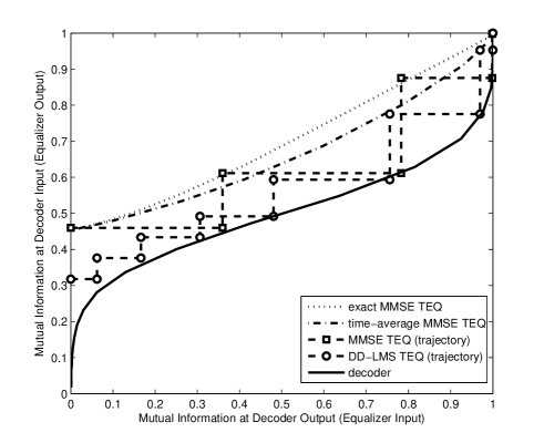
Figure 3: The EXIT chart for the exact MMSE turbo equalizer, the LMS turbo equalizer and their trajectory in a time invariant ISI channel [0.227,0.46,0.688,0.46,0.227]Tsuperscript0.2270.460.6880.460.227𝑇[0.227,0.46,0.688,0.46,0.227]^{T}. Here, we have SNR=10dBSNR10𝑑𝐵\mbox{SNR}=10dB, N1=9,N2=5formulae-sequencesubscript𝑁19subscript𝑁25N_{1}=9,N_{2}=5, feedback filter length N+M1=19𝑁𝑀119N+M-1=19, data block length =8192absent8192=8192, training data length =2048absent2048=2048, μ=0.001𝜇0.001\mu=0.001, BPSK signaling, random interleaver and 1212\frac{1}{2} rate convolutional code with constraint length of 333.

Comparison of an exact MMSE turbo equalizer with/without channel estimation error and an MMSE turbo equalizer with the time averaged soft variances (i.e. when an ideal filter for the converged adaptive turbo equalizer is used) via the EXIT chart [21] is given in Fig. 3. As the adaptive turbo equalizer, a decision directed (DD) LMS turbo equalizer is used in the data transmission period, while LMS is run on the received signals for the first turbo iteration and on the received signals and training symbols for the rest of turbo iterations in the training period. Note that the tentative decisions can be taken as the hard decisions at the output of the linear equalizer or as the soft decisions from the total LLRs at the output of decoder. When we consider nonideality, both of the MMSE turbo equalizer with channel estimation error and DD-LMS turbo equalizer loose mutual information at the equalizer in first few turbo iterations 222This performance loss in the first few turbo iterations can fail the iterative process in low SNR region. Even though there is a loss in mutual information at the equalizer in the first and second turbo iteration due to using decision directed data or channel estimation error, both algorithms follow their ideal performance at the end. (i.e., the DD LMS turbo equalizer can achieve the performance of the time-average MMSE turbo equalizer as the decision data gets more reliable). However, there is still a gap in achieved mutual information between the exact MMSE turbo equalizer and the LMS adaptive turbo equalizer except for the no a priori information and perfect a priori information cases. Note that such a gap can make an adaptive turbo equalizer become trapped at lower SNR region while an MMSE turbo equalizer converges as turbo iteration increases.

To remedy this, in the next section, we introduce piecewise linear equalizers to approximate 𝒲()𝒲{\cal W}(\cdot) and (){\cal F}(\cdot). We first discuss adaptive piecewise linear equalizers with a fixed partition of N+M2superscript𝑁𝑀2\mathbbm{C}^{N+M-2} (where 𝒒N+M2𝒒superscript𝑁𝑀2\mbox{$\mbox{\boldmath${q}$}$}\in\mathbbm{C}^{N+M-2}). Then, we introduce adaptive piecewise linear equalizers using context trees that can learn the best partition from a large class of possible partitions of N+M2superscript𝑁𝑀2\mathbbm{C}^{N+M-2}.

III Nonlinear Turbo Equalization Using Piecewise Linear Models

III-A Piecewise Linear Turbo Equalization with Fixed Partitioning

In this section, we divide the space spanned by 𝒒[0,1]N+M2𝒒superscript01𝑁𝑀2\mbox{$\mbox{\boldmath${q}$}$}\in[0,1]^{N+M-2} (assuming BPSK signaling for notational simplicity) into disjoint regions Vksubscript𝑉𝑘V_{k}, e.g., [0,1]N+M2=k=1KVksuperscript01𝑁𝑀2superscriptsubscript𝑘1𝐾subscript𝑉𝑘[0,1]^{N+M-2}=\bigcup_{k=1}^{K}V_{k} for some K𝐾K and train an independent linear equalizer in each region Vksubscript𝑉𝑘V_{k} to yield a final piecewise linear equalizer to approximate 𝒘=𝒲(𝒒)𝒘𝒲𝒒\mbox{\boldmath${w}$}={\cal W}(\mbox{$\mbox{\boldmath${q}$}$}) and 𝒇=(𝒒)𝒇𝒒\mbox{\boldmath${f}$}={\cal F}(\mbox{$\mbox{\boldmath${q}$}$}). As an example, given K𝐾K such regions, suppose a time varying linear equalizer is assigned to each region as 𝒘k(t)subscript𝒘𝑘𝑡\mbox{\boldmath${w}$}_{k}(t), 𝒇k(t)subscript𝒇𝑘𝑡\mbox{\boldmath${f}$}_{k}(t), k=1,,K𝑘1𝐾k=1,\ldots,K, such that at each time t𝑡t, if 𝒒(t)Vk𝒒𝑡subscript𝑉𝑘\mbox{$\mbox{\boldmath${q}$}$}(t)\in V_{k}, the estimate of the received signal is given as

x^k(t)=𝒘kT(t)𝒚(t)𝒇kT(t)𝒙¯(t)superscriptsubscript^𝑥𝑘𝑡superscriptsubscript𝒘𝑘𝑇𝑡𝒚𝑡superscriptsubscript𝒇𝑘𝑇𝑡¯𝒙𝑡\displaystyle\hat{x}_{k}(t)\stackrel{{\scriptstyle\bigtriangleup}}{{=}}\mbox{\boldmath${w}$}_{k}^{T}(t)\mbox{$\mbox{\boldmath${y}$}$}(t)-\mbox{\boldmath${f}$}_{k}^{T}(t)\mbox{$\bar{\mbox{\boldmath${x}$}}$}(t) (6)
x^(t)=x^k(t).^𝑥𝑡subscript^𝑥𝑘𝑡\displaystyle\hat{x}(t)=\hat{x}_{k}(t).

We emphasize that the time variations in 𝒘k(t)subscript𝒘𝑘𝑡\mbox{\boldmath${w}$}_{k}(t) and 𝒇k(t)subscript𝒇𝑘𝑡\mbox{\boldmath${f}$}_{k}(t) in (6) are not due to the time variation in 𝒒(t)𝒒𝑡\mbox{$\mbox{\boldmath${q}$}$}(t) unlike (3). The filters 𝒘k(t)subscript𝒘𝑘𝑡\mbox{\boldmath${w}$}_{k}(t) and 𝒇k(t)subscript𝒇𝑘𝑡\mbox{\boldmath${f}$}_{k}(t) are time varying since they are produced by adaptive algorithms sequentially learning the corresponding functions 𝒲()𝒲{\cal W}(\cdot) and (){\cal F}(\cdot) in region Vksubscript𝑉𝑘V_{k}. Note that if K𝐾K is large and the regions are dense such that 𝒲(𝒒)𝒲𝒒{\cal W}(\mbox{$\mbox{\boldmath${q}$}$}) (and (𝒒)𝒒{\cal F}(\mbox{$\mbox{\boldmath${q}$}$})) can be considered constant in Vksubscript𝑉𝑘V_{k}, say equal to 𝒲(𝒒k)𝒲subscript𝒒𝑘{\cal W}(\mbox{$\mbox{\boldmath${q}$}$}_{k}) for some 𝒒ksubscript𝒒𝑘\mbox{$\mbox{\boldmath${q}$}$}_{k} in region Vksubscript𝑉𝑘V_{k}, then if the adaptation method used in each region converges successfully, this yields 𝒘k(t)𝒲(𝒒k)subscript𝒘𝑘𝑡𝒲subscript𝒒𝑘\mbox{\boldmath${w}$}_{k}(t)\rightarrow{\cal W}(\mbox{$\mbox{\boldmath${q}$}$}_{k}) and 𝒇k(t)(𝒒k)subscript𝒇𝑘𝑡subscript𝒒𝑘\mbox{\boldmath${f}$}_{k}(t)\rightarrow{\cal F}(\mbox{$\mbox{\boldmath${q}$}$}_{k}) as t𝑡t\rightarrow\infty. Hence, if these regions are dense and there is enough data to learn the corresponding models in each region, then this piecewise model can approximate any smoothly varying 𝒲(𝒒)𝒲𝒒{\cal W}(\mbox{$\mbox{\boldmath${q}$}$}) and (𝒒)𝒒{\cal F}(\mbox{$\mbox{\boldmath${q}$}$}) [22].

In order to choose the corresponding regions V1,,VKsubscript𝑉1subscript𝑉𝐾V_{1},\ldots,V_{K}, we apply a vector quantization (VQ) algorithm to the sequence of {𝒒(t)}𝒒𝑡\{\mbox{\boldmath${q}$}(t)\}, such as the LBG VQ algorithm [23]. If a VQ algorithm with K𝐾K regions and Euclidean distance is used for clustering, then the centroids and the corresponding regions are defined as

𝒒~k=t,𝒒(t)Vk𝒒(t)t,𝒒(t)Vk1,superscriptsubscript~𝒒𝑘subscript𝑡𝒒𝑡subscript𝑉𝑘𝒒𝑡subscript𝑡𝒒𝑡subscript𝑉𝑘1\displaystyle\tilde{\mbox{\boldmath${q}$}}_{k}\stackrel{{\scriptstyle\bigtriangleup}}{{=}}\frac{\sum_{t,\mbox{$\mbox{\boldmath${q}$}$}(t)\in V_{k}}\mbox{$\mbox{\boldmath${q}$}$}(t)}{\sum_{t,\mbox{$\mbox{\boldmath${q}$}$}(t)\in V_{k}}1}, (7)
Vk={𝒒:𝒒𝒒~k𝒒𝒒~i,i=1,,K,ik},superscriptsubscript𝑉𝑘conditional-set𝒒formulae-sequencenorm𝒒subscript~𝒒𝑘norm𝒒subscript~𝒒𝑖formulae-sequence𝑖1𝐾𝑖𝑘\displaystyle V_{k}\stackrel{{\scriptstyle\bigtriangleup}}{{=}}\{\mbox{$\mbox{\boldmath${q}$}$}:\|\mbox{$\mbox{\boldmath${q}$}$}-\tilde{\mbox{\boldmath${q}$}}_{k}\|\leq\|\mbox{$\mbox{\boldmath${q}$}$}-\tilde{\mbox{\boldmath${q}$}}_{i}\|,i=1,\ldots,K,i\neq k\}, (8)

where 𝒒(t)=[q(tMN2+1),,q(t1),q(t+1),,q(t+N1)]T𝒒𝑡superscript𝑞𝑡𝑀subscript𝑁21𝑞𝑡1𝑞𝑡1𝑞𝑡subscript𝑁1𝑇\mbox{$\mbox{\boldmath${q}$}$}(t)=[q(t-M-N_{2}+1),\ldots,q(t-1),q(t+1),\ldots,q(t+N_{1})]^{T}, and 𝒒N+M2𝒒superscript𝑁𝑀2\mbox{$\mbox{\boldmath${q}$}$}\in\mathbbm{C}^{N+M-2}. We emphasize that we use a VQ algorithm on {𝒒(t)}𝒒𝑡\{\mbox{\boldmath${q}$}(t)\} to construct the corresponding partitioned regions in order to concentrate on 𝒒𝒒{q} vectors that are in {𝒒(t)}𝒒𝑡\{\mbox{\boldmath${q}$}(t)\} since 𝒲()𝒲{\cal W}(\cdot) and (){\cal F}(\cdot) should only be learned around 𝒒{𝒒(t)}𝒒𝒒𝑡\mbox{$\mbox{\boldmath${q}$}$}\in\mbox{$\{\mbox{\boldmath${q}$}(t)\}$}, not for all N+M2superscript𝑁𝑀2\mathbbm{C}^{N+M-2}. After the regions are constructed using the VQ algorithm and the corresponding filters in each region are trained with an appropriate adaptive method, the estimate of x(t)𝑥𝑡x(t) at each time t𝑡t is given as x^(t)=x^i(t)^𝑥𝑡subscript^𝑥𝑖𝑡\hat{x}(t)=\hat{x}_{i}(t) if i=argmink𝒒(t)𝒒~k𝑖subscript𝑘norm𝒒𝑡subscript~𝒒𝑘i=\arg\min_{k}\|\mbox{$\mbox{\boldmath${q}$}$}(t)-\tilde{\mbox{\boldmath${q}$}}_{k}\|.

A Pseudo-code of Piecewise Linear Turbo Equalizer:
% 111st iteration:
for t=1,,n𝑡1𝑛t=1,\ldots,n:
            x^(t)=𝒘(1)T(t)𝒚(t)^𝑥𝑡superscript𝒘1𝑇𝑡𝒚𝑡\hat{x}(t)=\mbox{\boldmath${w}$}^{(1)T}(t)\mbox{$\mbox{\boldmath${y}$}$}(t),
            if tT𝑡𝑇t\leq T: e(t)=x(t)x^(t)𝑒𝑡𝑥𝑡^𝑥𝑡e(t)=x(t)-\hat{x}(t), elseif t>T𝑡𝑇t>T: e(t)=Q(x^(t))x^(t)𝑒𝑡𝑄^𝑥𝑡^𝑥𝑡e(t)=Q(\hat{x}(t))-\hat{x}(t), Q()𝑄Q(\cdot) is a quantizer.
            𝒘(1)(t+1)=𝒘(1)(t)+μe(t)𝒚(t).superscript𝒘1𝑡1superscript𝒘1𝑡𝜇𝑒𝑡𝒚𝑡\mbox{\boldmath${w}$}^{(1)}(t+1)=\mbox{\boldmath${w}$}^{(1)}(t)+\mu e(t)\mbox{$\mbox{\boldmath${y}$}$}(t).
calculate 𝒒(t)𝒒𝑡\mbox{$\mbox{\boldmath${q}$}$}(t) using the SISO decoder for t>T𝑡𝑇t>T.
% 222nd iteration:
apply LBG VQ algorithm to {𝒒(t)}t>Tsubscript𝒒𝑡𝑡𝑇\mbox{$\{\mbox{\boldmath${q}$}(t)\}$}_{t>T} to generate 𝒒~k(2)superscriptsubscript~𝒒𝑘2\tilde{\mbox{\boldmath${q}$}}_{k}^{(2)}, k=1,,K𝑘1𝐾k=1,\ldots,K.
for k=1,,K𝑘1𝐾k=1,\ldots,K: 𝒘k(2)(0)=𝒘(1)(n)superscriptsubscript𝒘𝑘20superscript𝒘1𝑛\mbox{\boldmath${w}$}_{k}^{(2)}(0)=\mbox{\boldmath${w}$}^{(1)}(n), where 𝒘(1)(n)superscript𝒘1𝑛\mbox{\boldmath${w}$}^{(1)}(n) is from 1st iteration. (line A)
for t=1,,T𝑡1𝑇t=1,\ldots,T:
            for k=1,,K𝑘1𝐾k=1,\ldots,K:
                     ek(t)=x(t)𝒘k(2)T(t)𝒚(t)𝒇k(2)T(t)[𝑰diag(𝒒~k(2))]1/2𝒙(t)subscript𝑒𝑘𝑡𝑥𝑡subscriptsuperscript𝒘2𝑇𝑘𝑡𝒚𝑡subscriptsuperscript𝒇2𝑇𝑘𝑡superscriptdelimited-[]𝑰diagsuperscriptsubscript~𝒒𝑘212𝒙𝑡e_{k}(t)=x(t)-\mbox{\boldmath${w}$}^{(2)T}_{k}(t)\mbox{$\mbox{\boldmath${y}$}$}(t)-\mbox{\boldmath${f}$}^{(2)T}_{k}(t)[\mbox{\boldmath${I}$}-\mathrm{diag}(\tilde{\mbox{\boldmath${q}$}}_{k}^{(2)})]^{1/2}\mbox{$\mbox{\boldmath${x}$}$}(t), (line B)
                     𝒘k(2)(t+1)=𝒘k(2)(t)+μek(t)𝒚(t)superscriptsubscript𝒘𝑘2𝑡1superscriptsubscript𝒘𝑘2𝑡𝜇subscript𝑒𝑘𝑡𝒚𝑡\mbox{\boldmath${w}$}_{k}^{(2)}(t+1)=\mbox{\boldmath${w}$}_{k}^{(2)}(t)+\mu e_{k}(t)\mbox{$\mbox{\boldmath${y}$}$}(t), 𝒇k(2)(t+1)=𝒇k(2)(t)+μek(t)[𝑰diag(𝒒~k(2))]1/2𝒙(t).superscriptsubscript𝒇𝑘2𝑡1superscriptsubscript𝒇𝑘2𝑡𝜇subscript𝑒𝑘𝑡superscriptdelimited-[]𝑰diagsuperscriptsubscript~𝒒𝑘212𝒙𝑡\mbox{\boldmath${f}$}_{k}^{(2)}(t+1)=\mbox{\boldmath${f}$}_{k}^{(2)}(t)+\mu e_{k}(t)[\mbox{\boldmath${I}$}-\mathrm{diag}(\tilde{\mbox{\boldmath${q}$}}_{k}^{(2)})]^{1/2}\mbox{$\mbox{\boldmath${x}$}$}(t).
for t=T+1,,n𝑡𝑇1𝑛t=T+1,\ldots,n:
            i=argmink𝒒(t)𝒒~k(2)𝑖subscript𝑘norm𝒒𝑡superscriptsubscript~𝒒𝑘2i=\arg\min_{k}\|\mbox{$\mbox{\boldmath${q}$}$}(t)-\tilde{\mbox{\boldmath${q}$}}_{k}^{(2)}\|,
            x^(t)=𝒘i(2)T(t)𝒚(t)𝒇i(2)T(t)𝒙¯(t)^𝑥𝑡subscriptsuperscript𝒘2𝑇𝑖𝑡𝒚𝑡subscriptsuperscript𝒇2𝑇𝑖𝑡¯𝒙𝑡\hat{x}(t)=\mbox{\boldmath${w}$}^{(2)T}_{i}(t)\mbox{$\mbox{\boldmath${y}$}$}(t)-\mbox{\boldmath${f}$}^{(2)T}_{i}(t)\mbox{$\bar{\mbox{\boldmath${x}$}}$}(t),
            e(t)=Q(x^(t))x^(t)𝑒𝑡𝑄^𝑥𝑡^𝑥𝑡e(t)=Q(\hat{x}(t))-\hat{x}(t),
            𝒘i(2)(t+1)=𝒘i(2)(t)+μe(t)𝒚(t)superscriptsubscript𝒘𝑖2𝑡1superscriptsubscript𝒘𝑖2𝑡𝜇𝑒𝑡𝒚𝑡\mbox{\boldmath${w}$}_{i}^{(2)}(t+1)=\mbox{\boldmath${w}$}_{i}^{(2)}(t)+\mu e(t)\mbox{$\mbox{\boldmath${y}$}$}(t), 𝒇i(2)(t+1)=𝒇i(2)(t)+μe(t)𝒙¯(t).superscriptsubscript𝒇𝑖2𝑡1superscriptsubscript𝒇𝑖2𝑡𝜇𝑒𝑡¯𝒙𝑡\mbox{\boldmath${f}$}_{i}^{(2)}(t+1)=\mbox{\boldmath${f}$}_{i}^{(2)}(t)+\mu e(t)\mbox{$\bar{\mbox{\boldmath${x}$}}$}(t).
calculate {𝒒(t)}t>Tsubscript𝒒𝑡𝑡𝑇\mbox{$\{\mbox{\boldmath${q}$}(t)\}$}_{t>T} using the SISO decoder.
% m𝑚mth iteration:
apply LBG VQ algorithm to {𝒒(t)}t>Tsubscript𝒒𝑡𝑡𝑇\mbox{$\{\mbox{\boldmath${q}$}(t)\}$}_{t>T} to generate 𝒒~k(m)superscriptsubscript~𝒒𝑘𝑚\tilde{\mbox{\boldmath${q}$}}_{k}^{(m)}, k=1,,K𝑘1𝐾k=1,\ldots,K.
for k=1,,K𝑘1𝐾k=1,\ldots,K: 𝒘k(m)(0)=𝒘j(m1)(n)superscriptsubscript𝒘𝑘𝑚0superscriptsubscript𝒘𝑗𝑚1𝑛\mbox{\boldmath${w}$}_{k}^{(m)}(0)=\mbox{\boldmath${w}$}_{j}^{(m-1)}(n), 𝒇k(m)(0)=𝒇j(m1)(n)superscriptsubscript𝒇𝑘𝑚0superscriptsubscript𝒇𝑗𝑚1𝑛\mbox{\boldmath${f}$}_{k}^{(m)}(0)=\mbox{\boldmath${f}$}_{j}^{(m-1)}(n), where j=argmini𝒒~k(m)𝒒~i(m1)𝑗subscript𝑖normsuperscriptsubscript~𝒒𝑘𝑚superscriptsubscript~𝒒𝑖𝑚1j=\arg\min_{i}\|\tilde{\mbox{\boldmath${q}$}}_{k}^{(m)}-\tilde{\mbox{\boldmath${q}$}}_{i}^{(m-1)}\|. (line C)
for t=1,,T𝑡1𝑇t=1,\ldots,T:
            for k=1,,K𝑘1𝐾k=1,\ldots,K:
                     ek(t)=x(t)𝒘k(m)T(t)𝒚(t)𝒇k(m)T(t)[𝑰diag(𝒒~k)]1/2𝒙(t)subscript𝑒𝑘𝑡𝑥𝑡subscriptsuperscript𝒘𝑚𝑇𝑘𝑡𝒚𝑡subscriptsuperscript𝒇𝑚𝑇𝑘𝑡superscriptdelimited-[]𝑰diagsubscript~𝒒𝑘12𝒙𝑡e_{k}(t)=x(t)-\mbox{\boldmath${w}$}^{(m)T}_{k}(t)\mbox{$\mbox{\boldmath${y}$}$}(t)-\mbox{\boldmath${f}$}^{(m)T}_{k}(t)[\mbox{\boldmath${I}$}-\mathrm{diag}(\tilde{\mbox{\boldmath${q}$}}_{k})]^{1/2}\mbox{$\mbox{\boldmath${x}$}$}(t),
                     𝒘k(m)(t+1)=𝒘k(m)(t)+μek(t)𝒚(t)superscriptsubscript𝒘𝑘𝑚𝑡1superscriptsubscript𝒘𝑘𝑚𝑡𝜇subscript𝑒𝑘𝑡𝒚𝑡\mbox{\boldmath${w}$}_{k}^{(m)}(t+1)=\mbox{\boldmath${w}$}_{k}^{(m)}(t)+\mu e_{k}(t)\mbox{$\mbox{\boldmath${y}$}$}(t), 𝒇k(m)(t+1)=𝒇k(m)(t)+μek(t)[𝑰diag(𝒒~k(m))]1/2𝒙(t).superscriptsubscript𝒇𝑘𝑚𝑡1superscriptsubscript𝒇𝑘𝑚𝑡𝜇subscript𝑒𝑘𝑡superscriptdelimited-[]𝑰diagsuperscriptsubscript~𝒒𝑘𝑚12𝒙𝑡\mbox{\boldmath${f}$}_{k}^{(m)}(t+1)=\mbox{\boldmath${f}$}_{k}^{(m)}(t)+\mu e_{k}(t)[\mbox{\boldmath${I}$}-\mathrm{diag}(\tilde{\mbox{\boldmath${q}$}}_{k}^{(m)})]^{1/2}\mbox{$\mbox{\boldmath${x}$}$}(t).
for t=T+1,,n𝑡𝑇1𝑛t=T+1,\ldots,n,
            i=argmink𝒒(t)𝒒~k(m)𝑖subscript𝑘norm𝒒𝑡superscriptsubscript~𝒒𝑘𝑚i=\arg\min_{k}\|\mbox{$\mbox{\boldmath${q}$}$}(t)-\tilde{\mbox{\boldmath${q}$}}_{k}^{(m)}\|,
            x^(t)=𝒘i(m)T(t)𝒚(t)𝒇i(m)T(t)𝒙¯(t)^𝑥𝑡subscriptsuperscript𝒘𝑚𝑇𝑖𝑡𝒚𝑡subscriptsuperscript𝒇𝑚𝑇𝑖𝑡¯𝒙𝑡\hat{x}(t)=\mbox{\boldmath${w}$}^{(m)T}_{i}(t)\mbox{$\mbox{\boldmath${y}$}$}(t)-\mbox{\boldmath${f}$}^{(m)T}_{i}(t)\mbox{$\bar{\mbox{\boldmath${x}$}}$}(t),
            e(t)=Q(x^(t))x^(t)𝑒𝑡𝑄^𝑥𝑡^𝑥𝑡e(t)=Q(\hat{x}(t))-\hat{x}(t),
            𝒘i(m)(t+1)=𝒘i(m)(t)+μe(t)𝒚(t)superscriptsubscript𝒘𝑖𝑚𝑡1superscriptsubscript𝒘𝑖𝑚𝑡𝜇𝑒𝑡𝒚𝑡\mbox{\boldmath${w}$}_{i}^{(m)}(t+1)=\mbox{\boldmath${w}$}_{i}^{(m)}(t)+\mu e(t)\mbox{$\mbox{\boldmath${y}$}$}(t), 𝒇i(m)(t+1)=𝒇i(m)(t)+μe(t)𝒙¯(t).superscriptsubscript𝒇𝑖𝑚𝑡1superscriptsubscript𝒇𝑖𝑚𝑡𝜇𝑒𝑡¯𝒙𝑡\mbox{\boldmath${f}$}_{i}^{(m)}(t+1)=\mbox{\boldmath${f}$}_{i}^{(m)}(t)+\mu e(t)\mbox{$\bar{\mbox{\boldmath${x}$}}$}(t).
calculate {𝒒(t)}t>Tsubscript𝒒𝑡𝑡𝑇\mbox{$\{\mbox{\boldmath${q}$}(t)\}$}_{t>T} using the SISO decoder.
Figure 4: A piecewise linear equalizer for turbo equalization. This algorithm requires O(M+N)𝑂𝑀𝑁O(M+N) computations.

In Fig. 4, we introduce such a sequential piecewise linear equalizer that uses the LMS update to train its equalizer filters. Here, μ𝜇\mu is the learning rate of the LMS updates. One can use different adaptive methods instead of the LMS update, such as the RLS or NLMS updates [24], by only changing the filter update steps in Fig. 4. The algorithm of Fig. 4 has access to training data of size T𝑇T. After the training data is used, the adaptive methods work in decision directed mode [24]. Since there are no a priori probabilities in the first turbo iteration, this algorithm uses an LMS update to train a linear equalizer with only the feedforward filter, i.e., x^(t)=𝒘T(t)𝒚(t)^𝑥𝑡superscript𝒘𝑇𝑡𝒚𝑡\hat{x}(t)=\mbox{\boldmath${w}$}^{T}(t)\mbox{$\mbox{\boldmath${y}$}$}(t), without any regions or mean vectors. Note that an adaptive feedforward linear filter 𝒘(t)𝒘𝑡\mbox{\boldmath${w}$}(t) trained on only {y(t)}𝑦𝑡\{y(t)\} without a priori probabilities (as in the first iteration) converges to [11] (assuming zero variance in convergence)

limt𝒘(t)=𝒘o=[𝒗H(σn2𝑰+𝑯r𝑯rH+𝒗𝒗H)1]T,subscript𝑡𝒘𝑡subscript𝒘𝑜superscriptsuperscriptdelimited-[]superscript𝒗𝐻superscriptsuperscriptsubscript𝜎𝑛2𝑰subscript𝑯𝑟superscriptsubscript𝑯𝑟𝐻superscript𝒗𝒗𝐻1𝑇\lim_{t\rightarrow\infty}\mbox{\boldmath${w}$}(t)=\mbox{\boldmath${w}$}_{o}\stackrel{{\scriptstyle\bigtriangleup}}{{=}}[\mbox{$\mbox{\boldmath${v}$}$}^{H}(\sigma_{n}^{2}\mbox{\boldmath${I}$}+\mbox{\boldmath${H}$}_{r}\mbox{\boldmath${H}$}_{r}^{H}+\mbox{$\mbox{\boldmath${v}$}$}\mbox{$\mbox{\boldmath${v}$}$}^{H})^{-1}]^{T},

which is the linear MMSE feedforward filter in (2) with 𝑸(t)=𝑰𝑸𝑡𝑰\mbox{\boldmath${Q}$}(t)=\mbox{\boldmath${I}$}.

In the pseudo-code in Fig. 4, the iteration numbers are displayed as superscripts, e.g., 𝒘i(m)(t)subscriptsuperscript𝒘𝑚𝑖𝑡\mbox{\boldmath${w}$}^{(m)}_{i}(t), 𝒇i(m)(t)subscriptsuperscript𝒇𝑚𝑖𝑡\mbox{\boldmath${f}$}^{(m)}_{i}(t) are the feedforward and feedback filters for the m𝑚mth iteration corresponding to the i𝑖ith region, respectively. After the first iteration when {𝒒(t)}𝒒𝑡\{\mbox{\boldmath${q}$}(t)\} become available, we apply the VQ algorithm to get the corresponding regions and the centroids. Then, for each region, we run a separate LMS update to train a linear equalizer and construct the estimated data as in (6). In the start of the second iteration, in line A, each feedforward filter is initialized by the feedforward filter trained in the first iteration. Furthermore, although the linear equalizers should have the form 𝒘kT(t)𝒚(t)𝒇kT(t)𝒙¯(t)superscriptsubscript𝒘𝑘𝑇𝑡𝒚𝑡superscriptsubscript𝒇𝑘𝑇𝑡¯𝒙𝑡\mbox{\boldmath${w}$}_{k}^{T}(t)\mbox{$\mbox{\boldmath${y}$}$}(t)-\mbox{\boldmath${f}$}_{k}^{T}(t)\mbox{$\bar{\mbox{\boldmath${x}$}}$}(t), since we have the correct 𝒙(t)𝒙𝑡\mbox{$\mbox{\boldmath${x}$}$}(t) in the training mode for t=1,,T𝑡1𝑇t=1,\ldots,T, the algorithms are trained using 𝒘kT(t)𝒚(t)𝒇kT(t)[𝑰diag(𝒒~k)]1/2𝒙(t)superscriptsubscript𝒘𝑘𝑇𝑡𝒚𝑡superscriptsubscript𝒇𝑘𝑇𝑡superscriptdelimited-[]𝑰diagsubscript~𝒒𝑘12𝒙𝑡\mbox{\boldmath${w}$}_{k}^{T}(t)\mbox{$\mbox{\boldmath${y}$}$}(t)-\mbox{\boldmath${f}$}_{k}^{T}(t)[\mbox{\boldmath${I}$}-\mathrm{diag}(\tilde{\mbox{\boldmath${q}$}}_{k})]^{1/2}\mbox{$\mbox{\boldmath${x}$}$}(t) in (line B), i.e., 𝒙(t)𝒙𝑡\mbox{$\mbox{\boldmath${x}$}$}(t) is scaled using [𝑰diag(𝒒~k)]1/2superscriptdelimited-[]𝑰diagsubscript~𝒒𝑘12[\mbox{\boldmath${I}$}-\mathrm{diag}(\tilde{\mbox{\boldmath${q}$}}_{k})]^{1/2}, to incorporate the uncertainty during training [25]. After the second iteration, in the start of each iteration, in line C, the linear equalizers in each region, say k𝑘k, are initialized using the filters trained in the previous iteration that are closest to the k𝑘kth region, i.e., j=argmini𝒒~k(m)𝒒~i(m1)𝑗subscript𝑖normsuperscriptsubscript~𝒒𝑘𝑚superscriptsubscript~𝒒𝑖𝑚1j=\arg\min_{i}\|\tilde{\mbox{\boldmath${q}$}}_{k}^{(m)}-\tilde{\mbox{\boldmath${q}$}}_{i}^{(m-1)}\|, 𝒘k(m)(0)=𝒘j(m1)(n)superscriptsubscript𝒘𝑘𝑚0superscriptsubscript𝒘𝑗𝑚1𝑛\mbox{\boldmath${w}$}_{k}^{(m)}(0)=\mbox{\boldmath${w}$}_{j}^{(m-1)}(n), and 𝒇k(m)(0)=𝒇j(m1)(n)superscriptsubscript𝒇𝑘𝑚0superscriptsubscript𝒇𝑗𝑚1𝑛\mbox{\boldmath${f}$}_{k}^{(m)}(0)=\mbox{\boldmath${f}$}_{j}^{(m-1)}(n).

Assuming large K𝐾K with dense regions, we have 𝒒(t)𝒒~k𝒒𝑡subscript~𝒒𝑘\mbox{$\mbox{\boldmath${q}$}$}(t)\approx\tilde{\mbox{\boldmath${q}$}}_{k} when 𝒒(t)Vk𝒒𝑡subscript𝑉𝑘\mbox{$\mbox{\boldmath${q}$}$}(t)\in V_{k}. To get the vectors that the LMS trained linear filters in region k𝑘k eventually converge, i.e., the linear MMSE estimators assuming stationary 𝒙¯¯𝒙\bar{\mbox{\boldmath${x}$}}, we need to calculate E[(𝒙(t)𝒙¯(t))(𝒙(t)𝒙¯(t))H:𝒒(t)=𝒒~k]E[(\mbox{$\mbox{\boldmath${x}$}$}(t)-\mbox{$\bar{\mbox{\boldmath${x}$}}$}(t))(\mbox{$\mbox{\boldmath${x}$}$}(t)-\mbox{$\bar{\mbox{\boldmath${x}$}}$}(t))^{H}:\mbox{$\mbox{\boldmath${q}$}$}(t)=\tilde{\mbox{\boldmath${q}$}}_{k}], which is assumed to be diagonal due to the interleaving [11], yielding

E{[𝒙(t)𝒙¯(t)][𝒙(t)𝒙¯(t)]H:𝒒(t)=𝒒~k}𝐸conditional-setdelimited-[]𝒙𝑡¯𝒙𝑡superscriptdelimited-[]𝒙𝑡¯𝒙𝑡𝐻𝒒𝑡subscript~𝒒𝑘\displaystyle E\{[\mbox{$\mbox{\boldmath${x}$}$}(t)-\mbox{$\bar{\mbox{\boldmath${x}$}}$}(t)][\mbox{$\mbox{\boldmath${x}$}$}(t)-\mbox{$\bar{\mbox{\boldmath${x}$}}$}(t)]^{H}:\mbox{$\mbox{\boldmath${q}$}$}(t)=\tilde{\mbox{\boldmath${q}$}}_{k}\}
=E{E{[𝒙(t)𝒙¯(t)][𝒙(t)𝒙¯(t)]H:{LLRaE(t)},𝒒(t)=𝒒~k}:𝒒(t)=𝒒~k}absent𝐸conditional-set𝐸conditional-setdelimited-[]𝒙𝑡¯𝒙𝑡superscriptdelimited-[]𝒙𝑡¯𝒙𝑡𝐻superscriptsubscriptLLR𝑎𝐸𝑡𝒒𝑡subscript~𝒒𝑘𝒒𝑡subscript~𝒒𝑘\displaystyle=E\bigg{\{}E\big{\{}[\mbox{$\mbox{\boldmath${x}$}$}(t)-\mbox{$\bar{\mbox{\boldmath${x}$}}$}(t)][\mbox{$\mbox{\boldmath${x}$}$}(t)-\mbox{$\bar{\mbox{\boldmath${x}$}}$}(t)]^{H}\>:\>\{\mathrm{LLR}_{a}^{E}(t)\},\mbox{$\mbox{\boldmath${q}$}$}(t)=\tilde{\mbox{\boldmath${q}$}}_{k}\big{\}}\>:\>\mbox{$\mbox{\boldmath${q}$}$}(t)=\tilde{\mbox{\boldmath${q}$}}_{k}\bigg{\}}
=diag{[𝒒~k(1),,𝒒~k(M+N21),1,𝒒~k(M+N2),,𝒒~k(M+N2)]}absentdiagsubscript~𝒒𝑘1subscript~𝒒𝑘𝑀subscript𝑁211subscript~𝒒𝑘𝑀subscript𝑁2subscript~𝒒𝑘𝑀𝑁2\displaystyle=\mathrm{diag}\big{\{}[\tilde{\mbox{\boldmath${q}$}}_{k}(1),\ldots,\tilde{\mbox{\boldmath${q}$}}_{k}(M+N_{2}-1),1,\tilde{\mbox{\boldmath${q}$}}_{k}(M+N_{2}),\ldots,\tilde{\mbox{\boldmath${q}$}}_{k}(M+N-2)]\big{\}}

due to the definition of 𝒒(t)𝒒𝑡\mbox{$\mbox{\boldmath${q}$}$}(t) and assuming stationary distribution on x¯(t)¯𝑥𝑡\bar{x}(t). This yields that the linear filters in region k𝑘k converge to

limt𝒘k(t)=𝒘k,o=[𝒗H(σn2𝑰+𝑯r𝑸~k𝑯rH+𝒗𝒗H)1]T,subscript𝑡subscript𝒘𝑘𝑡subscript𝒘𝑘𝑜superscriptsuperscriptdelimited-[]superscript𝒗𝐻superscriptsuperscriptsubscript𝜎𝑛2𝑰subscript𝑯𝑟subscript~𝑸𝑘superscriptsubscript𝑯𝑟𝐻superscript𝒗𝒗𝐻1𝑇\displaystyle\lim_{t\rightarrow\infty}\mbox{\boldmath${w}$}_{k}(t)=\mbox{\boldmath${w}$}_{k,o}\stackrel{{\scriptstyle\bigtriangleup}}{{=}}[\mbox{$\mbox{\boldmath${v}$}$}^{H}(\sigma_{n}^{2}\mbox{\boldmath${I}$}+\mbox{\boldmath${H}$}_{r}\tilde{\mbox{\boldmath${Q}$}}_{k}\mbox{\boldmath${H}$}_{r}^{H}+\mbox{$\mbox{\boldmath${v}$}$}\mbox{$\mbox{\boldmath${v}$}$}^{H})^{-1}]^{T},
limt𝒇k(t)=𝒇k,o=𝑯T𝒘k,o,subscript𝑡subscript𝒇𝑘𝑡subscript𝒇𝑘𝑜superscriptsuperscript𝑯𝑇subscript𝒘𝑘𝑜\displaystyle\lim_{t\rightarrow\infty}\mbox{\boldmath${f}$}_{k}(t)=\mbox{\boldmath${f}$}_{k,o}\stackrel{{\scriptstyle\bigtriangleup}}{{=}}\mbox{\boldmath${H}$}^{T}\mbox{\boldmath${w}$}_{k,o}, (9)

where 𝑸~k=diag(𝒒~k)superscriptsubscript~𝑸𝑘diagsubscript~𝒒𝑘\tilde{\mbox{\boldmath${Q}$}}_{k}\stackrel{{\scriptstyle\bigtriangleup}}{{=}}\mathrm{diag}(\tilde{\mbox{\boldmath${q}$}}_{k}), assuming zero variance at convergence. Hence, at each time t𝑡t, assuming convergence, the difference between the MSE of the equalizer in (9) and the MSE of the linear MMSE equalizer in (2) is given by

𝒘k,oT𝑯r𝑸(t)𝑯rH𝒘k,o+σn2𝒘k,oT𝒘k,o[1𝒗H(σn2𝑰+𝑯r𝑸(t)𝑯rH+𝒗𝒗H)1𝒗]O(𝒒(t)𝒒~k),normsuperscriptsubscript𝒘𝑘𝑜𝑇subscript𝑯𝑟𝑸𝑡superscriptsubscript𝑯𝑟𝐻superscriptsubscript𝒘𝑘𝑜superscriptsubscript𝜎𝑛2superscriptsubscript𝒘𝑘𝑜𝑇superscriptsubscript𝒘𝑘𝑜delimited-[]1superscript𝒗𝐻superscriptsuperscriptsubscript𝜎𝑛2𝑰subscript𝑯𝑟𝑸𝑡superscriptsubscript𝑯𝑟𝐻superscript𝒗𝒗𝐻1𝒗𝑂norm𝒒𝑡subscript~𝒒𝑘\|\mbox{\boldmath${w}$}_{k,o}^{T}\mbox{\boldmath${H}$}_{r}\mbox{\boldmath${Q}$}(t)\mbox{\boldmath${H}$}_{r}^{H}\mbox{\boldmath${w}$}_{k,o}^{*}+\sigma_{n}^{2}\mbox{\boldmath${w}$}_{k,o}^{T}\mbox{\boldmath${w}$}_{k,o}^{*}-[1-\mbox{$\mbox{\boldmath${v}$}$}^{H}(\sigma_{n}^{2}\mbox{\boldmath${I}$}+\mbox{\boldmath${H}$}_{r}\mbox{\boldmath${Q}$}(t)\mbox{\boldmath${H}$}_{r}^{H}+\mbox{$\mbox{\boldmath${v}$}$}\mbox{$\mbox{\boldmath${v}$}$}^{H})^{-1}\mbox{$\mbox{\boldmath${v}$}$}]\|\leq O(\|\mbox{$\mbox{\boldmath${q}$}$}(t)-\tilde{\mbox{\boldmath${q}$}}_{k}\|), (10)

as shown in Appendix A. Due to (10) as the number of piecewise linear regions, i.e., K𝐾K, increases and 𝒒(t)𝒒~knorm𝒒𝑡subscript~𝒒𝑘\|\mbox{$\mbox{\boldmath${q}$}$}(t)-\tilde{\mbox{\boldmath${q}$}}_{k}\| approaches to 00, the MSE of the converged adaptive filter more accurately approximates the MSE of the linear MMSE equalizer.

In the algorithm of Fig. 4, the partition of the space of 𝒒[0,1]N+M2𝒒superscript01𝑁𝑀2\mbox{$\mbox{\boldmath${q}$}$}\in[0,1]^{N+M-2} is fixed, i.e., partitioned regions are fixed at the start of the equalization, after the VQ algorithm, and we sequentially learn a different linear equalizer for each region. Since the equalizers are sequentially learned with a limited amount of data, these may cause training problems if there is not enough data in each region. In other words, although one can increase K𝐾K to increase approximation power, if there is not enough data to learn the corresponding linear models in each region, this may deteriorate the performance. To alleviate this, one can try a piecewise linear model with smaller K𝐾K in the start of the learning and gradually increase K𝐾K to moderate values if enough data is available. In the next section, we examine the context tree weighting method that intrinsically does such weighting among different models based on their performance, hence, allowing the boundaries of the partition regions to be design parameters.

III-B Piecewise Linear Turbo Equalization Using Context Trees

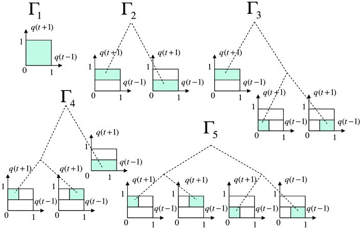
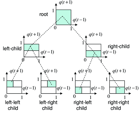
We first introduce a binary context tree to partition [0,1]N+M2superscript01𝑁𝑀2[0,1]^{N+M-2} into disjoint regions in order to construct a piecewise linear equalizer that can choose both the regions as well as the equalizer coefficients in these regions based on the equalization performance. On a context tree, starting from the root node, we have a left hand child and a right hand child. Each left hand child and right hand child have their own left hand and right hand children. This splitting yields a binary tree of depth D𝐷D with a total of 2Dsuperscript2𝐷2^{D} leaves at depth D𝐷D and 2D+11superscript2𝐷112^{D+1}-1 nodes. As an example, the context tree with D=2𝐷2D=2 in Fig. 5 partitions [0,1]2superscript012[0,1]^{2}, i.e., 𝒒=[q(t1),q(t+1)]T[0,1]2𝒒superscript𝑞𝑡1𝑞𝑡1𝑇superscript012\mbox{$\mbox{\boldmath${q}$}$}=[q(t-1),q(t+1)]^{T}\in[0,1]^{2}, into 444 disjoint regions. Each one of these 444 disjoint regions is assigned to a leaf on this binary tree. Then, recursively, each internal node on this tree represents a region (shaded areas in Fig. 5), which is the union of the regions assigned to its children.

On a binary context tree of depth D𝐷D, one can define a doubly exponential number, m1.52D𝑚superscript1.5superscript2𝐷m\approx 1.5^{2^{D}}, of “complete” subtrees as in Fig. 6. A complete subtree is constructed from a subset of the nodes of the original tree, starting from the same root node, and the union of the regions assigned to its leaves yields [0,1]N+M2superscript01𝑁𝑀2[0,1]^{N+M-2}. For example, for a subtree i𝑖i, if the regions assigned to its leaves are labeled as V1,i,,VKi,isubscript𝑉1𝑖subscript𝑉subscript𝐾𝑖𝑖V_{1,i},\ldots,V_{K_{i},i} where Kisubscript𝐾𝑖K_{i} is the number of leaves of the subtree i𝑖i, then [0,1]N+M2=k=1KiVk,isuperscript01𝑁𝑀2superscriptsubscript𝑘1subscript𝐾𝑖subscript𝑉𝑘𝑖[0,1]^{N+M-2}=\bigcup_{k=1}^{K_{i}}V_{k,i}. Each Vk,isubscript𝑉𝑘𝑖V_{k,i} of the subtree corresponds to a node in the original tree.
Refer to caption

Figure 5: A full binary context tree with depth, D=2𝐷2D=2, with 4 leaves. The leaves of this binary tree partitions [0,1]2superscript012[0,1]^{2}, i.e., [q(t1)q(t+1)][0,1]2delimited-[]𝑞𝑡1𝑞𝑡1superscript012[q(t-1)\;\;q(t+1)]\in[0,1]^{2}, into 4 disjoint regions.

Refer to caption

Figure 6: All partitions of [0,1]2superscript012[0,1]^{2} using binary context tree with D=2𝐷2D=2. Given any partition, the union of the regions represented by the leaves of each partition is equal to [0,1]2superscript012[0,1]^{2}.

With this definition, a complete subtree with the regions assigned to its leaves defines a complete “partition” of [0,1]N+M2superscript01𝑁𝑀2[0,1]^{N+M-2}. Continuing with our example, on a binary tree of depth D=2𝐷2D=2, we have 555 different partitions of [0,1]2superscript012[0,1]^{2} as shown in Fig. 6 labeled as Γ1,,Γ5subscriptΓ1subscriptΓ5{\Gamma}_{1},\ldots,{\Gamma}_{5}.

A Pseudo-code of Piecewise Linear Turbo Equalizer Using Context Trees:
% 111st iteration:
for t=1,,n𝑡1𝑛t=1,\ldots,n:
            x^ctw(t)=𝒘(1)T(t)𝒚(t)subscript^𝑥ctw𝑡superscript𝒘1𝑇𝑡𝒚𝑡\hat{x}_{\mathrm{ctw}}(t)=\mbox{\boldmath${w}$}^{(1)T}(t)\mbox{$\mbox{\boldmath${y}$}$}(t),
            if tT𝑡𝑇t\leq T: e(t)=x(t)x^(t)𝑒𝑡𝑥𝑡^𝑥𝑡e(t)=x(t)-\hat{x}(t).
            elseif t>T𝑡𝑇t>T: e(t)=Q(x^(t))x^(t)𝑒𝑡𝑄^𝑥𝑡^𝑥𝑡e(t)=Q(\hat{x}(t))-\hat{x}(t), Q()𝑄Q(\cdot) is a quantizer.
            𝒘(1)(t+1)=𝒘(1)(t)+μe(t)𝒚(t).superscript𝒘1𝑡1superscript𝒘1𝑡𝜇𝑒𝑡𝒚𝑡\mbox{\boldmath${w}$}^{(1)}(t+1)=\mbox{\boldmath${w}$}^{(1)}(t)+\mu e(t)\mbox{$\mbox{\boldmath${y}$}$}(t).
calculate 𝒒(t)𝒒𝑡\mbox{$\mbox{\boldmath${q}$}$}(t) using the SISO decoder for t>T𝑡𝑇t>T.
% m𝑚mth iteration:
apply LBG VQ algorithm to {𝒒(t)}t>Tsubscript𝒒𝑡𝑡𝑇\mbox{$\{\mbox{\boldmath${q}$}(t)\}$}_{t>T} to generate 𝒒~k(2)superscriptsubscript~𝒒𝑘2\tilde{\mbox{\boldmath${q}$}}_{k}^{(2)}, k=1,,2D𝑘1superscript2𝐷k=1,\ldots,2^{D} and 𝒒~k(2)superscriptsubscript~𝒒𝑘2\tilde{\mbox{\boldmath${q}$}}_{k}^{(2)}, k=2D+1,,2D+11𝑘superscript2𝐷1superscript2𝐷11k=2^{D}+1,\ldots,2^{D+1}-1.
if m==2m==2:
             for k=1,,2D+11𝑘1superscript2𝐷11k=1,\ldots,2^{D+1}-1: 𝒘k(2)(1)=𝒘(1)(n)superscriptsubscript𝒘𝑘21superscript𝒘1𝑛\mbox{\boldmath${w}$}_{k}^{(2)}(1)=\mbox{\boldmath${w}$}^{(1)}(n), where 𝒘(1)(n)superscript𝒘1𝑛\mbox{\boldmath${w}$}^{(1)}(n) is from 1st iteration.
if m3𝑚3m\geq 3:
             for i=1,,2D+11𝑖1superscript2𝐷11i=1,\ldots,2^{D+1}-1: 𝒘k(m)(1)=𝒘j(m1)(n)superscriptsubscript𝒘𝑘𝑚1superscriptsubscript𝒘𝑗𝑚1𝑛\mbox{\boldmath${w}$}_{k}^{(m)}(1)=\mbox{\boldmath${w}$}_{j}^{(m-1)}(n), 𝒇k(m)(1)=𝒇j(m1)(n)superscriptsubscript𝒇𝑘𝑚1superscriptsubscript𝒇𝑗𝑚1𝑛\mbox{\boldmath${f}$}_{k}^{(m)}(1)=\mbox{\boldmath${f}$}_{j}^{(m-1)}(n), where j=argmini𝒒~k(m)𝒒~i(m1)𝑗subscript𝑖normsuperscriptsubscript~𝒒𝑘𝑚superscriptsubscript~𝒒𝑖𝑚1j=\arg\min_{i}\|\tilde{\mbox{\boldmath${q}$}}_{k}^{(m)}-\tilde{\mbox{\boldmath${q}$}}_{i}^{(m-1)}\|.
for k=1,,2D+11𝑘1superscript2𝐷11k=1,\ldots,2^{D+1}-1: Ak(0)=1subscript𝐴𝑘01A_{k}(0)=1, Bk(0)=1subscript𝐵𝑘01B_{k}(0)=1. (line A)
for t=1,,T𝑡1𝑇t=1,\ldots,T:
            for i=1,,2D𝑖1superscript2𝐷i=1,\ldots,2^{D}:
                     𝒙¯(t)=[𝑰diag(𝒒~k(m))]1/2𝒙(t)superscript¯𝒙𝑡superscriptdelimited-[]𝑰diagsuperscriptsubscript~𝒒𝑘𝑚12𝒙𝑡\bar{\mbox{$\mbox{\boldmath${x}$}$}}(t)\stackrel{{\scriptstyle\bigtriangleup}}{{=}}[\mbox{\boldmath${I}$}-\mathrm{diag}(\tilde{\mbox{\boldmath${q}$}}_{k}^{(m)})]^{1/2}\mbox{$\mbox{\boldmath${x}$}$}(t) %to consider uncertainty during training
                     𝒍(1)=i𝒍1𝑖\mbox{\boldmath${l}$}(1)=i, where 𝒍𝒍{l} corresponds dark nodes starting from the leaf node i𝑖i
                     η1(t)=1/2subscript𝜂1𝑡12\eta_{1}(t)=1/2.
                     for l=2,,D+1𝑙2𝐷1l=2,\ldots,D+1:
                              ηl(t)=12As(t1)ηl1(t)subscript𝜂𝑙𝑡12subscript𝐴𝑠𝑡1subscript𝜂𝑙1𝑡\eta_{l}(t)=\frac{1}{2}A_{s}(t-1)\eta_{l-1}(t), where s𝑠s is a sibling node of 𝒍(l)𝒍𝑙\mbox{\boldmath${l}$}(l), i.e., VsV𝒍(l)=V𝒍(l1)subscript𝑉𝑠subscript𝑉𝒍𝑙subscript𝑉𝒍𝑙1V_{s}\bigcup V_{\mbox{\boldmath${l}$}(l)}=V_{\mbox{\boldmath${l}$}(l-1)},
                              βl(t)=ηl(t)B𝒍(l)(t1)A𝒍(1)(t1)subscript𝛽𝑙𝑡subscript𝜂𝑙𝑡subscript𝐵𝒍𝑙𝑡1subscript𝐴𝒍1𝑡1\beta_{l}(t)=\frac{\eta_{l}(t)B_{\mbox{\boldmath${l}$}(l)}(t-1)}{A_{\mbox{\boldmath${l}$}(1)}(t-1)}. (line B)
                     for l=D+1,,1𝑙𝐷11l=D+1,\ldots,1:
                              e𝒍(l)(t)=x(t)[𝒘𝒍(l)(m)T(t)𝒚(t)𝒇𝒍(l)(m)T(t)𝒙¯(t)]subscript𝑒𝒍𝑙𝑡𝑥𝑡delimited-[]subscriptsuperscript𝒘𝑚𝑇𝒍𝑙𝑡𝒚𝑡subscriptsuperscript𝒇𝑚𝑇𝒍𝑙𝑡¯𝒙𝑡e_{\mbox{\boldmath${l}$}(l)}(t)=x(t)-[\mbox{\boldmath${w}$}^{(m)T}_{\mbox{\boldmath${l}$}(l)}(t)\mbox{$\mbox{\boldmath${y}$}$}(t)-\mbox{\boldmath${f}$}^{(m)T}_{\mbox{\boldmath${l}$}(l)}(t)\mbox{$\bar{\mbox{\boldmath${x}$}}$}(t)],
                              B𝒍(l)(t)=B𝒍(l)(t1)exp(ce𝒍(l)(t)2)subscript𝐵𝒍𝑙𝑡subscript𝐵𝒍𝑙𝑡1𝑐superscriptnormsubscript𝑒𝒍𝑙𝑡2B_{\mbox{\boldmath${l}$}(l)}(t)=B_{\mbox{\boldmath${l}$}(l)}(t-1)\exp\left(-c\left\|{e_{\mbox{\boldmath${l}$}(l)}(t)}\right\|^{2}\right), % where c𝑐c is a positive constant, (line C)
                               if l=D+1𝑙𝐷1l=D+1: A𝒍(l)(t)=B𝒍(l)(t)subscript𝐴𝒍𝑙𝑡subscript𝐵𝒍𝑙𝑡A_{\mbox{\boldmath${l}$}(l)}(t)=B_{\mbox{\boldmath${l}$}(l)}(t), (line D)
                               else: A𝒍(l)(t)=12A𝒍(l),l(t1)A𝒍(l),r(t1)+12B𝒍(l)(t)subscript𝐴𝒍𝑙𝑡12subscript𝐴𝒍𝑙𝑙𝑡1subscript𝐴𝒍𝑙𝑟𝑡112subscript𝐵𝒍𝑙𝑡A_{\mbox{\boldmath${l}$}(l)}(t)=\frac{1}{2}A_{\mbox{\boldmath${l}$}(l),l}(t-1)A_{\mbox{\boldmath${l}$}(l),r}(t-1)+\frac{1}{2}B_{\mbox{\boldmath${l}$}(l)}(t), (line E)
                              % where (𝒍(l),l)𝒍𝑙𝑙(\mbox{\boldmath${l}$}(l),l) and (𝒍(l),r)𝒍𝑙𝑟(\mbox{\boldmath${l}$}(l),r) are the left and right hand children of 𝒍(l)𝒍𝑙\mbox{\boldmath${l}$}(l), respectively,
                              𝒘𝒍(l)(m)(t+1)=𝒘𝒍(l)(m)(t)+μe𝒍(l)(t)𝒚(t)superscriptsubscript𝒘𝒍𝑙𝑚𝑡1superscriptsubscript𝒘𝒍𝑙𝑚𝑡𝜇subscript𝑒𝒍𝑙𝑡𝒚𝑡\mbox{\boldmath${w}$}_{\mbox{\boldmath${l}$}(l)}^{(m)}(t+1)=\mbox{\boldmath${w}$}_{\mbox{\boldmath${l}$}(l)}^{(m)}(t)+\mu e_{\mbox{\boldmath${l}$}(l)}(t)\mbox{$\mbox{\boldmath${y}$}$}(t), 𝒇𝒍(l)(m)(t+1)=𝒇𝒍(l)(m)(t)+μe𝒍(l)(t)𝒙¯(t).superscriptsubscript𝒇𝒍𝑙𝑚𝑡1superscriptsubscript𝒇𝒍𝑙𝑚𝑡𝜇subscript𝑒𝒍𝑙𝑡¯𝒙𝑡\mbox{\boldmath${f}$}_{\mbox{\boldmath${l}$}(l)}^{(m)}(t+1)=\mbox{\boldmath${f}$}_{\mbox{\boldmath${l}$}(l)}^{(m)}(t)+\mu e_{\mbox{\boldmath${l}$}(l)}(t)\mbox{$\bar{\mbox{\boldmath${x}$}}$}(t).
for t=T+1,,n𝑡𝑇1𝑛t=T+1,\ldots,n:
            i=argmink𝒒(t)𝒒~k(m)𝑖subscript𝑘norm𝒒𝑡superscriptsubscript~𝒒𝑘𝑚i=\arg\min_{k}\|\mbox{$\mbox{\boldmath${q}$}$}(t)-\tilde{\mbox{\boldmath${q}$}}_{k}^{(m)}\|, k=1,,2D𝑘1superscript2𝐷k=1,\ldots,2^{D}.
            find nodes that i𝑖i belongs to and store them in 𝒍𝒍{l} starting from the leaf node i𝑖i, i.e., 𝒍(1)=i𝒍1𝑖\mbox{\boldmath${l}$}(1)=i.
            η1(t)=1/2subscript𝜂1𝑡12\eta_{1}(t)=1/2,
            for l=2,,D+1𝑙2𝐷1l=2,\ldots,D+1:
                     ηl(t)=12As(t)ηl1(t)subscript𝜂𝑙𝑡12subscript𝐴𝑠𝑡subscript𝜂𝑙1𝑡\eta_{l}(t)=\frac{1}{2}A_{s}(t)\eta_{l-1}(t).
                     βl(t)=ηl(t)B𝒍(l)(t1)A𝒍(1)(t1)subscript𝛽𝑙𝑡subscript𝜂𝑙𝑡subscript𝐵𝒍𝑙𝑡1subscript𝐴𝒍1𝑡1\beta_{l}(t)=\frac{\eta_{l}(t)B_{\mbox{\boldmath${l}$}(l)}(t-1)}{A_{\mbox{\boldmath${l}$}(1)}(t-1)}.
            x^ctw(t)=k=1D+1βk(t)[𝒘𝒍(k)(m)T(t)𝒚(t)𝒇𝒍(k)(m)T(t)𝒙¯(t)]subscript^𝑥ctw𝑡superscriptsubscript𝑘1𝐷1subscript𝛽𝑘𝑡delimited-[]subscriptsuperscript𝒘𝑚𝑇𝒍𝑘𝑡𝒚𝑡subscriptsuperscript𝒇𝑚𝑇𝒍𝑘𝑡¯𝒙𝑡\hat{x}_{\mathrm{ctw}}(t)=\sum_{k=1}^{D+1}\beta_{k}(t)[\mbox{\boldmath${w}$}^{(m)T}_{\mbox{\boldmath${l}$}(k)}(t)\mbox{$\mbox{\boldmath${y}$}$}(t)-\mbox{\boldmath${f}$}^{(m)T}_{\mbox{\boldmath${l}$}(k)}(t)\mbox{$\bar{\mbox{\boldmath${x}$}}$}(t)], (line F)
            for l=D+1,,1𝑙𝐷11l=D+1,\ldots,1:
                     e𝒍(l)(t)=Q(x^ctw(t))[𝒘𝒍(l)(m)T(t)𝒚(t)𝒇𝒍(l)(m)T(t)𝒙¯(t)]subscript𝑒𝒍𝑙𝑡𝑄subscript^𝑥ctw𝑡delimited-[]subscriptsuperscript𝒘𝑚𝑇𝒍𝑙𝑡𝒚𝑡subscriptsuperscript𝒇𝑚𝑇𝒍𝑙𝑡¯𝒙𝑡e_{\mbox{\boldmath${l}$}(l)}(t)=Q(\hat{x}_{\mathrm{ctw}}(t))-[\mbox{\boldmath${w}$}^{(m)T}_{\mbox{\boldmath${l}$}(l)}(t)\mbox{$\mbox{\boldmath${y}$}$}(t)-\mbox{\boldmath${f}$}^{(m)T}_{\mbox{\boldmath${l}$}(l)}(t)\mbox{$\bar{\mbox{\boldmath${x}$}}$}(t)], (line G)
                     B𝒍(l)(t+1)=B𝒍(l)(t1)exp(ce𝒍(l)(t)2)subscript𝐵𝒍𝑙𝑡1subscript𝐵𝒍𝑙𝑡1𝑐superscriptnormsubscript𝑒𝒍𝑙𝑡2B_{\mbox{\boldmath${l}$}(l)}(t+1)=B_{\mbox{\boldmath${l}$}(l)}(t-1)\exp\left(-c\left\|{e_{\mbox{\boldmath${l}$}(l)}(t)}\right\|^{2}\right),
                      if l=D+1𝑙𝐷1l=D+1: A𝒍(l)(t)=B𝒍(l)(t)subscript𝐴𝒍𝑙𝑡subscript𝐵𝒍𝑙𝑡A_{\mbox{\boldmath${l}$}(l)}(t)=B_{\mbox{\boldmath${l}$}(l)}(t),
                      else: A𝒍(l)(t)=12A𝒍(l),l(t1)A𝒍(l),r(t1)+12B𝒍(l)(t)subscript𝐴𝒍𝑙𝑡12subscript𝐴𝒍𝑙𝑙𝑡1subscript𝐴𝒍𝑙𝑟𝑡112subscript𝐵𝒍𝑙𝑡A_{\mbox{\boldmath${l}$}(l)}(t)=\frac{1}{2}A_{\mbox{\boldmath${l}$}(l),l}(t-1)A_{\mbox{\boldmath${l}$}(l),r}(t-1)+\frac{1}{2}B_{\mbox{\boldmath${l}$}(l)}(t),
                     𝒘𝒍(l)(m)(t+1)=𝒘𝒍(l)(m)(t)+μe𝒍(l)(t)𝒚(t)superscriptsubscript𝒘𝒍𝑙𝑚𝑡1superscriptsubscript𝒘𝒍𝑙𝑚𝑡𝜇subscript𝑒𝒍𝑙𝑡𝒚𝑡\mbox{\boldmath${w}$}_{\mbox{\boldmath${l}$}(l)}^{(m)}(t+1)=\mbox{\boldmath${w}$}_{\mbox{\boldmath${l}$}(l)}^{(m)}(t)+\mu e_{\mbox{\boldmath${l}$}(l)}(t)\mbox{$\mbox{\boldmath${y}$}$}(t), 𝒇𝒍(l)(m)(t+1)=𝒇𝒍(l)(m)(t)+μe𝒍(l)(t)𝒙¯(t).superscriptsubscript𝒇𝒍𝑙𝑚𝑡1superscriptsubscript𝒇𝒍𝑙𝑚𝑡𝜇subscript𝑒𝒍𝑙𝑡¯𝒙𝑡\mbox{\boldmath${f}$}_{\mbox{\boldmath${l}$}(l)}^{(m)}(t+1)=\mbox{\boldmath${f}$}_{\mbox{\boldmath${l}$}(l)}^{(m)}(t)+\mu e_{\mbox{\boldmath${l}$}(l)}(t)\mbox{$\bar{\mbox{\boldmath${x}$}}$}(t).
calculate {𝒒(t)}t>Tsubscript𝒒𝑡𝑡𝑇\mbox{$\{\mbox{\boldmath${q}$}(t)\}$}_{t>T} using the SISO decoder.
Figure 7: A context tree based turbo equalization. This algorithm requires O(D(M+N))𝑂𝐷𝑀𝑁O\big{(}D(M+N)\big{)} computations.

As in the previous section, we partition regions with the LBG VQ algorithm and then construct our context tree over these regions as follows. Suppose the LBG VQ algorithm is applied to {𝒒(t)}𝒒𝑡\{\mbox{\boldmath${q}$}(t)\} with K=2D𝐾superscript2𝐷K=2^{D} to generate 2Dsuperscript2𝐷2^{D} regions [23]. The LBG VQ algorithm uses a tree notion similar to the context tree introduced in Fig. 6 such that the algorithm starts from a root node which calculates the mean of all the vectors in {𝒒(t)}𝒒𝑡\{\mbox{\boldmath${q}$}(t)\} as the root codeword, and binary splits the data as well as the root codeword into two segments. Then, these newly constructed codewords are iteratively used as the initial codebook of the split segments. These two codewords are then split in four and the process is repeated until the desired number of regions are reached. At the end, this binary splitting and clustering yield 2Dsuperscript2𝐷2^{D} regions with the corresponding centroids 𝒒~isubscript~𝒒𝑖\tilde{\mbox{\boldmath${q}$}}_{i}, i=1,,2D𝑖1superscript2𝐷i=1,\ldots,2^{D}, which are assigned to the leaves of the context tree. Note that since each couple of the leaves (or nodes) come from a parent node after a binary splitting, these parent codewords are stored as the internal nodes of the context tree, i.e., the nodes that are generated by splitting a parent node are considered as siblings of this parent node where the centroid before splitting is stored. Hence, in this sense, the LBG VQ algorithm intrinsically constructs the context tree. However, note that, at each turn, even though the initial centroids at each splitting directly come from the parent node in the original LBG VQ algorithm, the final regions of the leaf nodes while minimizing distortion by iterating (7) and (8) may invade the regions of the other parents nodes, i.e., the union of regions assigned to the children of the split parent node can be different than the region assigned to the parent node. Note that one can modify the LBG algorithm with the constraint that the region of the children nodes should be optimized within the regions of the their parent nodes. However, this constraint may deteriorate the performance due to more quantization error.

Given such a context tree, one can define m(1.5)2D𝑚superscript1.5superscript2𝐷m\approx(1.5)^{2^{D}} different partitions of the space spanned by 𝒒𝒒{q} and construct a piecewise linear equalizer as in Fig. 4 for each such partition. For each such partition, one can train and use a piecewise linear model. Note that all these piecewise linear equalizers are constructed using subsets of nodes ρ{1,,2D+11}𝜌1superscript2𝐷11\rho\in\{1,\ldots,2^{D+1}-1\}. Hence, suppose we number each node on this context tree ρ=1,,2D+11𝜌1superscript2𝐷11\rho=1,\ldots,2^{D+1}-1 and assign a linear equalizer to each node as x^ρ(t)=𝒘ρT(t)𝒚(t)𝒇ρT(t)𝒙¯(t)subscript^𝑥𝜌𝑡superscriptsubscript𝒘𝜌𝑇𝑡𝒚𝑡superscriptsubscript𝒇𝜌𝑇𝑡¯𝒙𝑡\hat{x}_{\rho}(t)=\mbox{\boldmath${w}$}_{\rho}^{T}(t)\mbox{$\mbox{\boldmath${y}$}$}(t)-\mbox{\boldmath${f}$}_{\rho}^{T}(t)\mbox{$\bar{\mbox{\boldmath${x}$}}$}(t). The linear models 𝒘ρsubscript𝒘𝜌\mbox{\boldmath${w}$}_{\rho}, 𝒇ρsubscript𝒇𝜌\mbox{\boldmath${f}$}_{\rho} that are assigned to node ρ𝜌\rho, train only on the data assigned to that node as in Fig. 4, i.e., if 𝒒(t)𝒒𝑡\mbox{$\mbox{\boldmath${q}$}$}(t) is in the region that is assigned to the node Vρsubscript𝑉𝜌V_{\rho} then 𝒘ρsubscript𝒘𝜌\mbox{\boldmath${w}$}_{\rho} and 𝒇ρsubscript𝒇𝜌\mbox{\boldmath${f}$}_{\rho} are updated. Then, the piecewise linear equalizer corresponding to the partition Γi={V1,i,,VKi,i}subscriptΓ𝑖subscript𝑉1𝑖subscript𝑉subscript𝐾𝑖𝑖{{\Gamma}}_{i}=\{V_{1,i},\ldots,V_{K_{i},i}\} (where l=1KiVk,i=[0,1]N+M2superscriptsubscript𝑙1subscript𝐾𝑖subscript𝑉𝑘𝑖superscript01𝑁𝑀2\bigcup_{l=1}^{K_{i}}V_{k,i}=[0,1]^{N+M-2}), say x^Γi(t)subscript^𝑥subscriptΓ𝑖𝑡\hat{x}_{{{\Gamma}}_{i}}(t), is defined such that if 𝒒(t)Vk,i𝒒𝑡subscript𝑉𝑘𝑖\mbox{$\mbox{\boldmath${q}$}$}(t)\in V_{k,i} and ρ𝜌\rho is the node that is assigned to Vk,isubscript𝑉𝑘𝑖V_{k,i} then

x^Γi(t)subscript^𝑥subscriptΓ𝑖𝑡\displaystyle\hat{x}_{{{\Gamma}}_{i}}(t) =x^ρ(t)absentsubscript^𝑥𝜌𝑡\displaystyle=\hat{x}_{\rho}(t)
=𝒘ρT(t)𝒚(t)𝒇ρT(t)𝒙¯(t).absentsuperscriptsubscript𝒘𝜌𝑇𝑡𝒚𝑡superscriptsubscript𝒇𝜌𝑇𝑡¯𝒙𝑡\displaystyle=\mbox{\boldmath${w}$}_{\rho}^{T}(t)\mbox{$\mbox{\boldmath${y}$}$}(t)-\mbox{\boldmath${f}$}_{\rho}^{T}(t)\mbox{$\bar{\mbox{\boldmath${x}$}}$}(t). (11)

One of these partitions, with the given piecewise adaptive linear model x^Γi(t)subscript^𝑥subscriptΓ𝑖𝑡\hat{x}_{{{\Gamma}}_{i}}(t) achieves the minimal loss, e.g., the minimal accumulated squared error t=1n(x(t)x^Γi(t))2superscriptsubscript𝑡1𝑛superscript𝑥𝑡subscript^𝑥subscriptΓ𝑖𝑡2\sum_{t=1}^{n}(x(t)-\hat{x}_{{{\Gamma}}_{i}}(t))^{2}, for some n𝑛n. However, the best piecewise model with the best partition is not known a priori. We next introduce an algorithm that achieves the performance of the best partition with the best linear model that achieves the minimal accumulated square-error with complexity only linear in the depth of the context tree per sample, i.e., complexity O(D(2N+M))𝑂𝐷2𝑁𝑀O\left(D(2N+M)\right) instead of O((1.5)2DD(2N+M))𝑂superscript1.5superscript2𝐷𝐷2𝑁𝑀O\left((1.5)^{2^{D}}D(2N+M)\right), where D𝐷D is the depth of the tree.

Remark 2: We emphasize that the partitioned model that corresponds to the union of the leaves, i.e., the finest partition, has the finest partition of the space of variances. Hence, it has the highest number of regions and parameters to model the nonlinear dependency. However, note that at each such region, the finest partition needs to train the corresponding linear equalizer that belongs to that region. As an example, the piecewise linear equalizer with the finest partition may not yield satisfactory results in the beginning of the adaptation if there is not enough data to train all the model parameters. In this sense, the context tree algorithm adaptively weights coarser and finer models based on their performance.

To accomplish this, we introduce the algorithm in Fig. 7, i.e., x^ctw(t)subscript^𝑥ctw𝑡\hat{x}_{\mathrm{ctw}}(t), that is constructed using the context tree weighting method introduced in [14]. The context tree based equalization algorithm implicitly constructs all x^Γi(t)subscript^𝑥subscriptΓ𝑖𝑡\hat{x}_{{{\Gamma}}_{i}}(t), i=1,,m𝑖1𝑚i=1,\ldots,m, piecewise linear equalizers and acts as if it had actually run all these equalizers in parallel on the received data. At each time t𝑡t, the final estimation x^ctw(t)subscript^𝑥ctw𝑡\hat{x}_{\mathrm{ctw}}(t) is constructed as a weighted combination of all the outputs x^Γi(t)subscript^𝑥subscriptΓ𝑖𝑡\hat{x}_{{{\Gamma}}_{i}}(t) of these piecewise linear equalizers, where the combination weights are calculated proportional to the performance of each equalizer x^Γi(t)subscript^𝑥subscriptΓ𝑖𝑡\hat{x}_{{{\Gamma}}_{i}}(t) on the past data. However, as shown in (11), although there are m𝑚m different piecewise linear algorithms, at each time t𝑡t, each x^Γi(t)subscript^𝑥subscriptΓ𝑖𝑡\hat{x}_{{{\Gamma}}_{i}}(t) is equal to one of the D𝐷D node estimations to which 𝒒(t)𝒒𝑡\mbox{$\mbox{\boldmath${q}$}$}(t) belongs, e.g., if 𝒒(t)𝒒𝑡\mbox{$\mbox{\boldmath${q}$}$}(t) belongs to the left-left hand child on Fig. 5, x^Γi(t)subscript^𝑥subscriptΓ𝑖𝑡\hat{x}_{{{\Gamma}}_{i}}(t), i=1,,m𝑖1𝑚i=1,\ldots,m, use either the node estimations x^ρ(t)subscript^𝑥𝜌𝑡\hat{x}_{\rho}(t) that belong to the left-left hand child or the left-hand child or the root. How the context tree algorithm keeps the track of these m𝑚m piecewise linear models as well as their performance-based combination weights with computational complexity only linear in the depth of the context tree is explained in Appendix B.

For the context tree algorithm, since there are no a priori probabilities in the first iteration, the first iteration of Fig. 7 is the same as the first iteration of Fig. 4. After the first iteration, to incorporate the uncertainty during training as in Fig. 4, the context tree algorithm is run by using weighted training data [25]. At each time t>T𝑡𝑇t>T, x^ctw(t)subscript^𝑥ctw𝑡\hat{x}_{\mathrm{ctw}}(t) constructs its nonlinear estimation of x(t)𝑥𝑡x(t) as follows. We first find the regions to which 𝒒(t)𝒒𝑡\mbox{$\mbox{\boldmath${q}$}$}(t) belongs. Due to the tree structure, one needs only find the leaf node in which 𝒒(t)𝒒𝑡\mbox{$\mbox{\boldmath${q}$}$}(t) lies and collect all the parent nodes towards the root node. The nodes to which 𝒒(t)𝒒𝑡\mbox{$\mbox{\boldmath${q}$}$}(t) belongs are stored in 𝒍𝒍{l} in Fig. 7. The final estimate x^ctw(t)subscript^𝑥ctw𝑡\hat{x}_{\mathrm{ctw}}(t) is constructed as a weighted combination of the estimates generated in these nodes, i.e., x^ρ(t)subscript^𝑥𝜌𝑡\hat{x}_{\rho}(t), ρ𝒍𝜌𝒍\rho\in\mbox{\boldmath${l}$}, where the weights are functions of the performance of the node estimates in previous samples. At each time t𝑡t, x^ctw(t)subscript^𝑥ctw𝑡\hat{x}_{\mathrm{ctw}}(t) requires O(ln(D))𝑂𝐷O(\ln(D)) calculations to find the leaf to which 𝒒(t)𝒒𝑡\mbox{$\mbox{\boldmath${q}$}$}(t) belongs. Then, D+1𝐷1D+1 node estimations, x^ρ(t)subscript^𝑥𝜌𝑡\hat{x}_{\rho}(t), ρ𝒍𝜌𝒍\rho\in\mbox{\boldmath${l}$}, are calculated and the filters at these nodes should be updated with O(2N+M)𝑂2𝑁𝑀O(2N+M) computations. The final weighted combination is produced with O(D)𝑂𝐷O(D) computations. Hence, at each time the context tree algorithm requires O(D(2N+M))𝑂𝐷2𝑁𝑀O(D(2N+M)) computational complexity. For this algorithm, we have the following result.

Theorem 2: Let {x(t)}𝑥𝑡\{x(t)\}, {n(t)}𝑛𝑡\{n(t)\} and {y(t)}𝑦𝑡\{y(t)\} represent the transmitted, noise and received signals and {𝐪(t)}𝐪𝑡\{\mbox{\boldmath${q}$}(t)\} represents the sequence of variances constructed using the a priori probabilities for each constellation point produced by the SISO decoder. Let x^ρ(t)subscript^𝑥𝜌𝑡\hat{x}_{\rho}(t), ρ=1,,2D+11𝜌1superscript2𝐷11\rho=1,\ldots,2^{D+1}-1, are estimates of x(t)𝑥𝑡x(t) produced by the equalizers assigned to each node on the context tree. The algorithm x^ctw(t)subscript^𝑥ctw𝑡\hat{x}_{\mathrm{ctw}}(t), when applied to {y(t)}𝑦𝑡\{y(t)\}, for all n𝑛n achieves

t=1n(x(t)x^ctw(t))2minΓi{t=1n[x(t)x^Γi(t)]2+2Ki1},superscriptsubscript𝑡1𝑛superscript𝑥𝑡subscript^𝑥ctw𝑡2subscriptsubscriptΓ𝑖superscriptsubscript𝑡1𝑛superscriptdelimited-[]𝑥𝑡subscript^𝑥subscriptΓ𝑖𝑡22subscript𝐾𝑖1\sum_{t=1}^{n}\big{(}x(t)-\hat{x}_{\mathrm{ctw}}(t)\big{)}^{2}\leq\min_{{{\Gamma}}_{i}}\left\{\sum_{t=1}^{n}\big{[}x(t)-\hat{x}_{{\Gamma}_{i}}(t)\big{]}^{2}+2K_{i}-1\right\}, (12)

for all i𝑖i, i=1,,m(1.5)2Dformulae-sequence𝑖1𝑚superscript1.5superscript2𝐷i=1,\ldots,m\approx(1.5)^{2^{D}}, assuming perfect feedback in decision directed mode i.e., Q(x^(t))=x(t)𝑄^𝑥𝑡𝑥𝑡Q(\hat{x}(t))=x(t) when tT𝑡𝑇t\geq T, where x^Γi(t)subscript^𝑥subscriptΓ𝑖𝑡\hat{x}_{{{\Gamma}}_{i}}(t) is the equalizer constructed as

x^Γi(t)=x^ρ(t),subscript^𝑥subscriptΓ𝑖𝑡subscript^𝑥𝜌𝑡\hat{x}_{{{\Gamma}}_{i}}(t)=\hat{x}_{\rho}(t),

ρ𝜌\rho is the node assigned to the volume in Γi={V1,i,,VKi,i}subscriptΓ𝑖subscript𝑉1𝑖subscript𝑉subscript𝐾𝑖𝑖{{\Gamma}}_{i}=\{V_{1,i},\ldots,V_{K_{i},i}\} such that 𝐪(t)𝐪𝑡\mbox{$\mbox{\boldmath${q}$}$}(t) belongs and Kisubscript𝐾𝑖K_{i} is the number of regions in ΓisubscriptΓ𝑖{\Gamma}_{i}. If the estimation algorithms assigned to each node are selected as adaptive linear equalizers such as an RLS update based algorithm, (12) yields

t=1n[x(t)x^ctw(t)]2mini{\displaystyle\sum_{t=1}^{n}\big{[}x(t)-\hat{x}_{\mathrm{ctw}}(t)\big{]}^{2}\leq\min_{i}\Bigg{\{} min𝒘k,iN,𝒇k,iN+M1k=1,,Kit=1n[x(t)𝒘si(t),iT𝒚(t)𝒇si(t),iT𝒙¯(t)]2+limit-fromsubscript𝑘1subscript𝐾𝑖formulae-sequencesubscript𝒘𝑘𝑖superscript𝑁subscript𝒇𝑘𝑖superscript𝑁𝑀1superscriptsubscript𝑡1𝑛superscriptdelimited-[]𝑥𝑡superscriptsubscript𝒘subscript𝑠𝑖𝑡𝑖𝑇𝒚𝑡superscriptsubscript𝒇subscript𝑠𝑖𝑡𝑖𝑇¯𝒙𝑡2\displaystyle\min_{\underset{k=1,\ldots,K_{i}}{\mbox{\boldmath${w}$}_{k,i}\in\mathbbm{C}^{N},\mbox{\boldmath${f}$}_{k,i}\in\mathbbm{C}^{N+M-1}}}\sum_{t=1}^{n}\big{[}x(t)-\mbox{\boldmath${w}$}_{s_{i}(t),i}^{T}\mbox{$\mbox{\boldmath${y}$}$}(t)-\mbox{\boldmath${f}$}_{s_{i}(t),i}^{T}\mbox{$\bar{\mbox{\boldmath${x}$}}$}(t)]^{2}+
O((2N+M)ln(n))+2Ki1}.\displaystyle O\big{(}(2N+M)\ln(n)\big{)}+2K_{i}-1\Bigg{\}}. (13)

where si(t)subscript𝑠𝑖𝑡s_{i}(t) is an indicator variable for ΓisubscriptΓ𝑖{\Gamma}_{i} such that if 𝐪(t)Vk,i𝐪𝑡subscript𝑉𝑘𝑖\mbox{$\mbox{\boldmath${q}$}$}(t)\in V_{k,i}, then si(t)=ksubscript𝑠𝑖𝑡𝑘s_{i}(t)=k.

An outline of the proof of this theorem is given in Appendix B.

Remark 3: We observe from (12) that the context tree algorithm achieves the performance of the best sequential algorithm among a doubly exponential number of possible algorithms. Note that the bound in (12) holds uniformly for all i𝑖i, however the bound is the largest for the finest partition corresponding to all leaves. We observe from (13) that the context tree algorithm also achieves the performance of even the best piecewise linear model, independently optimized in each region, for all i𝑖i when the node estimators in each regions are adaptive algorithms that achieve the minimum least square-error.

III-B1 MSE Performance of the Context Tree Equalizer

To get the MSE performance of the context tree equalizer, we observe that the result (13) in the theorem is uniformly true for any sequence {x(t)}𝑥𝑡\{x(t)\}. Hence, as a corollary to the theorem, taking the expectation of both sides of (13) with respect to any distribution on {x(t)}𝑥𝑡\{x(t)\} yields the following corollary:
Corollary:

t=1nE{[x(t)x^ctw(t)]2}minΓi{\displaystyle\sum_{t=1}^{n}E\left\{\big{[}x(t)-\hat{x}_{\mathrm{ctw}}(t)\big{]}^{2}\right\}\leq\min_{{{\Gamma}}_{i}}\Bigg{\{} min𝒘k,iN,𝒇k,iN+M1k=1,,Kit=1nE{[x(t)𝒘si(t),iT𝒚(t)𝒇si(t1),iT𝒙¯(t)]2}+limit-fromsubscript𝑘1subscript𝐾𝑖formulae-sequencesubscript𝒘𝑘𝑖superscript𝑁subscript𝒇𝑘𝑖superscript𝑁𝑀1superscriptsubscript𝑡1𝑛𝐸superscriptdelimited-[]𝑥𝑡superscriptsubscript𝒘subscript𝑠𝑖𝑡𝑖𝑇𝒚𝑡superscriptsubscript𝒇subscript𝑠𝑖𝑡1𝑖𝑇¯𝒙𝑡2\displaystyle\min_{\underset{k=1,\ldots,K_{i}}{\mbox{\boldmath${w}$}_{k,i}\in\mathbbm{C}^{N},\mbox{\boldmath${f}$}_{k,i}\in\mathbbm{C}^{N+M-1}}}\sum_{t=1}^{n}E\left\{\big{[}x(t)-\mbox{\boldmath${w}$}_{s_{i}(t),i}^{T}\mbox{$\mbox{\boldmath${y}$}$}(t)-\mbox{\boldmath${f}$}_{s_{i}(t-1),i}^{T}\mbox{$\bar{\mbox{\boldmath${x}$}}$}(t)]^{2}\right\}+
O((N+M)ln(n))+2Ki1}.\displaystyle O\big{(}(N+M)\ln(n)\big{)}+2K_{i}-1\Bigg{\}}. (14)

Note that (13) is true for all i𝑖i, and given i𝑖i for any 𝒘k,isubscript𝒘𝑘𝑖\mbox{\boldmath${w}$}_{k,i}, 𝒇k,isubscript𝒇𝑘𝑖\mbox{\boldmath${f}$}_{k,i}, i=1,,Ki𝑖1subscript𝐾𝑖i=1,\ldots,K_{i}, i.e.,

t=1n[x(t)x^ctw(t)]2t=1n[x(t)𝒘si(t),iT𝒚(t)𝒇si(t1),iT𝒙¯(t)]2+O((N+M)ln(n))+2Ki1,superscriptsubscript𝑡1𝑛superscriptdelimited-[]𝑥𝑡subscript^𝑥ctw𝑡2superscriptsubscript𝑡1𝑛superscriptdelimited-[]𝑥𝑡superscriptsubscript𝒘subscript𝑠𝑖𝑡𝑖𝑇𝒚𝑡superscriptsubscript𝒇subscript𝑠𝑖𝑡1𝑖𝑇¯𝒙𝑡2𝑂𝑁𝑀𝑛2subscript𝐾𝑖1\sum_{t=1}^{n}\big{[}x(t)-\hat{x}_{\mathrm{ctw}}(t)\big{]}^{2}\leq\sum_{t=1}^{n}\big{[}x(t)-\mbox{\boldmath${w}$}_{s_{i}(t),i}^{T}\mbox{$\mbox{\boldmath${y}$}$}(t)-\mbox{\boldmath${f}$}_{s_{i}(t-1),i}^{T}\mbox{$\bar{\mbox{\boldmath${x}$}}$}(t)\big{]}^{2}+O\big{(}(N+M)\ln(n)\big{)}+2K_{i}-1, (15)

since (13) is true for the minimizing i𝑖i and equalizer vectors. Taking the expectation of both sides of (15) and minimizing with respect to i𝑖i and 𝒘k,isubscript𝒘𝑘𝑖\mbox{\boldmath${w}$}_{k,i}, 𝒇k,isubscript𝒇𝑘𝑖\mbox{\boldmath${f}$}_{k,i}, i=1,,Ki𝑖1subscript𝐾𝑖i=1,\ldots,K_{i} yields the corollary.

We emphasize that the minimizer vectors 𝒘k,isubscript𝒘𝑘𝑖\mbox{\boldmath${w}$}_{k,i} and 𝒇k,isubscript𝒇𝑘𝑖\mbox{\boldmath${f}$}_{k,i} at the right hand side of (14) minimize the sum of all the MSEs. Hence, the corollary does not relate the MSE performance of the CTW equalizer to the MSE performance of the linear MMSE equalizer given in (2). However, if we assume that the adaptive filters trained at each node converge to their optimal coefficient vectors with zero variance and for sufficiently large D𝐷D and n𝑛n, we have for piecewise linear models such as for the finest partition

t=1n(x(t)x^Γ|K|(t))2t=1n{[x(t)𝒘s|K|(t),|K|,oT𝒚(t)𝒇s|K(t),|K|,oT𝒙¯(t)]2},\sum_{t=1}^{n}\big{(}x(t)-\hat{x}_{{{\Gamma}}_{|K|}}(t)\big{)}^{2}\approx\sum_{t=1}^{n}\left\{\big{[}x(t)-\mbox{\boldmath${w}$}_{s_{|K|}(t),|K|,o}^{T}\mbox{$\mbox{\boldmath${y}$}$}(t)-\mbox{\boldmath${f}$}_{s_{|K}(t),|K|,o}^{T}\mbox{$\bar{\mbox{\boldmath${x}$}}$}(t)\big{]}^{2}\right\}, (16)

where we assumed that, for notational simplicity, the |K|𝐾|K|th partition is the finest partition, 𝒘s|K|(t),|K|,osubscript𝒘subscript𝑠𝐾𝑡𝐾𝑜\mbox{\boldmath${w}$}_{s_{|K|}(t),|K|,o} and 𝒇s|K|(t),|K|,osubscript𝒇subscript𝑠𝐾𝑡𝐾𝑜\mbox{\boldmath${f}$}_{s_{|K|}(t),|K|,o} are the MSE optimal filters (if defined) corresponding to the regions assigned to the leaves of the context tree. Note that we require D𝐷D to be large such that we can assume 𝒒(t)𝒒𝑡\mbox{$\mbox{\boldmath${q}$}$}(t) to be constant in each region such that these MSE optimal filters are well-defined. Since (13) is correct for all partitions and for the minimizing 𝒘𝒘{w}, 𝒇𝒇{f} vectors, (13) holds for any 𝒘𝒘{w} and 𝒇𝒇{f}’s pairs including 𝒘s|K|(t),|K|,osubscript𝒘subscript𝑠𝐾𝑡𝐾𝑜\mbox{\boldmath${w}$}_{s_{|K|}(t),|K|,o} and 𝒇s|K|(t),|K|,osubscript𝒇subscript𝑠𝐾𝑡𝐾𝑜\mbox{\boldmath${f}$}_{s_{|K|}(t),|K|,o} pair. Since (13) in the theorem is uniformly true, taking the expectation preserves the bound and using (16), we have

1nt=1nE{[x(t)x^ctw(t)]2}1nt=1nE{[x(t)𝒘s|K|(t),|K|,oT𝒚(t)𝒇s|K(t),|K|,oT𝒙¯(t)]2}+O(2D+1n),\frac{1}{n}\sum_{t=1}^{n}E\left\{\big{[}x(t)-\hat{x}_{\mathrm{ctw}}(t)\big{]}^{2}\right\}\leq\frac{1}{n}\sum_{t=1}^{n}E\left\{\big{[}x(t)-\mbox{\boldmath${w}$}_{s_{|K|}(t),|K|,o}^{T}\mbox{$\mbox{\boldmath${y}$}$}(t)-\mbox{\boldmath${f}$}_{s_{|K}(t),|K|,o}^{T}\mbox{$\bar{\mbox{\boldmath${x}$}}$}(t)\big{]}^{2}\right\}+O\left(\frac{2^{D+1}}{n}\right), (17)

since for the finest partition K|K|=2Dsubscript𝐾𝐾superscript2𝐷K_{|K|}=2^{D}. Using the MSE definition for each node in (17) yields

1nt=1nE{[x(t)x^ctw(t)]2}1𝑛superscriptsubscript𝑡1𝑛𝐸superscriptdelimited-[]𝑥𝑡subscript^𝑥ctw𝑡2\displaystyle\frac{1}{n}\sum_{t=1}^{n}E\left\{\big{[}x(t)-\hat{x}_{\mathrm{ctw}}(t)\big{]}^{2}\right\}
1nt=1n{𝒘s|K|(t),|K|,oT𝑯r𝑸(t)𝑯rH𝒘s|K|(t),|K|,o+σn2𝒘s|K|(t),|K|,oT𝒘s|K|(t),|K|,o}+O(2D+1n)absent1𝑛superscriptsubscript𝑡1𝑛superscriptsubscript𝒘subscript𝑠𝐾𝑡𝐾𝑜𝑇subscript𝑯𝑟𝑸𝑡superscriptsubscript𝑯𝑟𝐻superscriptsubscript𝒘subscript𝑠𝐾𝑡𝐾𝑜superscriptsubscript𝜎𝑛2superscriptsubscript𝒘subscript𝑠𝐾𝑡𝐾𝑜𝑇superscriptsubscript𝒘subscript𝑠𝐾𝑡𝐾𝑜𝑂superscript2𝐷1𝑛\displaystyle\leq\frac{1}{n}\sum_{t=1}^{n}\left\{\mbox{\boldmath${w}$}_{s_{|K|}(t),|K|,o}^{T}\mbox{\boldmath${H}$}_{r}\mbox{\boldmath${Q}$}(t)\mbox{\boldmath${H}$}_{r}^{H}\mbox{\boldmath${w}$}_{s_{|K|}(t),|K|,o}^{*}+\sigma_{n}^{2}\mbox{\boldmath${w}$}_{s_{|K|}(t),|K|,o}^{T}\mbox{\boldmath${w}$}_{s_{|K|}(t),|K|,o}^{*}\right\}+O\left(\frac{2^{D+1}}{n}\right) (18)
1nt=1n{min𝒘,𝒇E{[x(t)𝒘T𝒚(t)𝒇T𝒙¯(t)]2|𝒒(t)}+O(12D)}+O(2D+1n),absent1𝑛superscriptsubscript𝑡1𝑛subscript𝒘𝒇𝐸conditional-setsuperscriptdelimited-[]𝑥𝑡superscript𝒘𝑇𝒚𝑡superscript𝒇𝑇¯𝒙𝑡2𝒒𝑡𝑂1superscript2𝐷𝑂superscript2𝐷1𝑛\displaystyle\leq\frac{1}{n}\sum_{t=1}^{n}\left\{\min_{\mbox{\boldmath${w}$},\mbox{\boldmath${f}$}}E\left\{\big{[}x(t)-\mbox{\boldmath${w}$}^{T}\mbox{$\mbox{\boldmath${y}$}$}(t)-\mbox{\boldmath${f}$}^{T}\mbox{$\bar{\mbox{\boldmath${x}$}}$}(t)\big{]}^{2}|\mbox{$\mbox{\boldmath${q}$}$}(t)\right\}+O\left(\frac{1}{2^{D}}\right)\right\}+O\left(\frac{2^{D+1}}{n}\right), (19)

where (19) follows from assuming large D𝐷D, the MSE in each node is bounded as in (10). Note that O(𝒒(t)𝒒~k)𝑂norm𝒒𝑡subscript~𝒒𝑘O(\|\mbox{$\mbox{\boldmath${q}$}$}(t)-\tilde{\mbox{$\mbox{\boldmath${q}$}$}}_{k}\|) at the right hand side of (10) can further be upper bounded by O(12D)𝑂1superscript2𝐷O\left(\frac{1}{2^{D}}\right) assuming large enough D𝐷D with the partition given in Fig. 5 since we have 2Dsuperscript2𝐷2^{D} regions and 𝒒(t)N+M2norm𝒒𝑡𝑁𝑀2\|\mbox{$\mbox{\boldmath${q}$}$}(t)\|\leq\sqrt{N+M-2}. Hence, as D𝐷D\rightarrow\infty, the context tree algorithm asymptotically achieves the performance of the linear MMSE equalizer, i.e., the equalizer that is nonlinear in the variances of the soft information.

IV Numerical Examples

In the following, we simulate the performance of the algorithms introduced in this paper under different scenarios. A rate one half convolutional code with constraint length 333 and random interleaving is used. In the first set of experiments, we use the time invariant channel from [7] (Chapter 10)

𝒉=[0.227,0.46,0.688,0.46,0.227]T𝒉superscript0.2270.460.6880.460.227𝑇\mbox{\boldmath${h}$}=[0.227,0.46,0.688,0.46,0.227]^{T}

with the training size T=1024𝑇1024T=1024 and data length 512051205120 (excluding training). The BERs and MSE curves are calculated over 202020 independent trials. The decision directed mode is used for all the LMS algorithms, e.g., for the ordinary LMS turbo equalizer we compete against and for all the node filters on the context tree. Our calculation of the extrinsic LLR at the output of the ordinary LMS algorithm is based on [9]. For all LMS filters, we use N1=9subscript𝑁19N_{1}=9, N2=5subscript𝑁25N_{2}=5, length N+M1=19𝑁𝑀119N+M-1=19 feedback filter. The learning rates for the LMS algorithms are set to μ=0.001𝜇0.001\mu=0.001. This learning rate is selected to guarantee the convergence of the ordinary LMS filter in the training part. The same learning rate is used directly on the context tree without tuning. In Fig. 8a, we demonstrate the time evaluation of the weight vector for the ordinary LMS turbo equalization algorithm in the first turbo iteration. We also plot the convolution of the channel 𝒉𝒉{h} and the converged weight vector of the LMS algorithm at the end of the first iteration in Fig. 8b. In Fig. 10, we plot BERs for an ordinary LMS algorithm, a context-tree equalization algorithm with D=2𝐷2D=2 given in Fig. 7 and the piecewise linear equalization algorithm with the finest partition, i.e., x^Γ|K|(t)subscript^𝑥subscriptΓ𝐾𝑡\hat{x}_{{{\Gamma}}_{|K|}}(t), on the same tree. Note that the piecewise linear equalizer with the finest partition, i.e., Γ5subscriptΓ5{\Gamma}_{5}, in Fig. 6, has the finest partition with the highest number of linear models, i.e., 2Dsuperscript2𝐷2^{D} independent filters, for equalization. However, we emphasize that all the linear filters in the leaves should be sequentially trained for the finest partition. Hence, as explained in Section III-B, the piecewise linear model with the finest partition may yield inferior performance compared to the CTW algorithm that adaptively weights all the models based on their performance. We observe that the context tree equalizer outperforms the ordinary LMS equalizer and the equalizer corresponding to the finest partition for these simulations. In Fig. 10, we plot the weight evaluation of the context tree algorithm, i.e., the combined weight in line F of Fig. 7, to show the convergence of the CTW algorithm. Note that the combined weight vector for the CTW algorithm is only defined over the data length period 512051205120 at each turbo iteration, i.e., the combined weight vector is not defined in the training period. We collect the combined weight vectors for the CTW algorithm in the data period for all iterations and plot them in Fig. 10. This results jumps in the figure, since at each discontinuity, i.e., after the data period, we switch to the training period and continue to train the node filters. The context tree algorithm, unlike the finest partition model, adaptively weights different partitions in each level. To see this, in Fig. 11a, we plot weights assigned to each level in a depth D=2𝐷2D=2 context tree. We also plot the time evaluation of the performance measures Aρ(t)subscript𝐴𝜌𝑡A_{\rho}(t) in Fig. 11b. We observe that the context tree algorithm, as expected, at the start of the equalization divides the weights fairly uniformly among the partitions or node equalizers. However, naturally, as the training size increases, when there is enough data to train all the node filters, the context tree algorithm favors models with better performance. Note that at each iteration, we reset node probabilities Aρ(t)=1subscript𝐴𝜌𝑡1A_{\rho}(t)=1 since a new tree is constructed using clustering.

To see the effect of depth on the performance of the context tree equalizer, we plot the for the same channel, BERs corresponding to context tree equalizers of depth, D=1𝐷1D=1, D=2𝐷2D=2 and D=3𝐷3D=3 in Fig. 13. We observe that as the depth of the tree increases the performance of the tree equalizer improves for these depth ranges. However, note that the computational complexity of the CTW equalizer is directly proportional to depth. As the last set of experiments, we perform the same set of experiments on a randomly generated channel of length 777 and plot the BERs in Fig. 13. We observe similar improvement in BER for this randomly generated channel for these simulations.
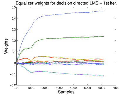
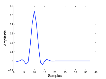
Refer to caption Refer to caption

                                   (a)                                                                      (b)

Figure 8: (a) Ensemble averaged weight vector for the DD LMS algorithm in the first turbo iteration, where μ=0.001𝜇0.001\mu=0.001, T=1024𝑇1024T=1024 and data length 512051205120. (b) Convolution of the trained weight vector of the DD LMS algorithm at sample 512051205120 and the channel 𝒉𝒉{h}.

Refer to caption

Figure 9: BERs for an ordinary DD LMS algorithm, a CTW equalizer with D=2𝐷2D=2 and tree given in Fig. 5, the piecewise equalizer with the finest partition, i.e., x^Γ5(t)subscript^𝑥subscriptΓ5𝑡\hat{x}_{{{\Gamma}}_{5}}(t), where μ=0.001𝜇0.001\mu=0.001, N1=9subscript𝑁19N_{1}=9, N2=5subscript𝑁25N_{2}=5, N+M1=19𝑁𝑀119N+M-1=19.

Refer to caption

Figure 10: Ensemble averaged combined weight vector for the CTW equalizer over 777 turbo iterations. Here, we have μ=0.001𝜇0.001\mu=0.001, T=1024𝑇1024T=1024, data length 512051205120 and 777 turbo iterations.

Refer to caption         Refer to caption

                                   (a)                                                                      (b)

Figure 11: (a) The distribution of the weights, i.e., values assigned to βi(t)subscript𝛽𝑖𝑡\beta_{i}(t), i=1,2,3𝑖123i=1,2,3, such that βi(t)subscript𝛽𝑖𝑡\beta_{i}(t) belongs to i𝑖ith level. (b) Time evaluation of Aρ(t)subscript𝐴𝜌𝑡A_{\rho}(t) which represents the performance of the linear equalizer assigned to node ρ𝜌\rho. Note that at each iteration, we reset Aρ(t)subscript𝐴𝜌𝑡A_{\rho}(t) since a new tree is constructed using clustering.

Refer to caption

Figure 12: BERs corresponding to CTW equalizers of depth D=1𝐷1D=1, D=2𝐷2D=2 and D=3𝐷3D=3.

Refer to caption

Figure 13: BERs for an ordinary DD LMS algorithm, a CTW equalizer with D=2𝐷2D=2 and tree given in Fig. 5, the piecewise equalizer with the finest partition, i.e., x^Γ5(t)subscript^𝑥subscriptΓ5𝑡\hat{x}_{{{\Gamma}}_{5}}(t), where μ=0.001𝜇0.001\mu=0.001, N1=9subscript𝑁19N_{1}=9, N2=5subscript𝑁25N_{2}=5, N+M1=19𝑁𝑀119N+M-1=19.

V Conclusion

In this paper, we introduced an adaptive nonlinear turbo equalization algorithm using context trees to model the nonlinear dependency of the linear MMSE equalizer on the soft information generated from the decoder. We use the CTW algorithm to partition the space of variances, which are time dependent and generated from the soft information. We demonstrate that the algorithm introduced asymptotically achieves the performance of the best piecewise linear model defined on this context tree with a computational complexity only of the order of an ordinary linear equalizer. We also demonstrate the convergence of the MSE of the CTW algorithm to the MSE of the linear minimum MSE estimator as the depth of the context tree and the data length increase. A) To calculate the difference between the MSE of the equalizer in (9) and the MSE of the linear MMSE equalizer in (2), we start with

𝒘k,oT𝑯r𝑸(t)𝑯rH𝒘k,o+σn2𝒘k,oT𝒘k,o[1𝒗H(σn2𝑰+𝑯r𝑸(t)𝑯rH+𝒗𝒗H)1𝒗]normsuperscriptsubscript𝒘𝑘𝑜𝑇subscript𝑯𝑟𝑸𝑡superscriptsubscript𝑯𝑟𝐻superscriptsubscript𝒘𝑘𝑜superscriptsubscript𝜎𝑛2superscriptsubscript𝒘𝑘𝑜𝑇superscriptsubscript𝒘𝑘𝑜delimited-[]1superscript𝒗𝐻superscriptsuperscriptsubscript𝜎𝑛2𝑰subscript𝑯𝑟𝑸𝑡superscriptsubscript𝑯𝑟𝐻superscript𝒗𝒗𝐻1𝒗\displaystyle\|\mbox{\boldmath${w}$}_{k,o}^{T}\mbox{\boldmath${H}$}_{r}\mbox{\boldmath${Q}$}(t)\mbox{\boldmath${H}$}_{r}^{H}\mbox{\boldmath${w}$}_{k,o}^{*}+\sigma_{n}^{2}\mbox{\boldmath${w}$}_{k,o}^{T}\mbox{\boldmath${w}$}_{k,o}^{*}-[1-\mbox{$\mbox{\boldmath${v}$}$}^{H}(\sigma_{n}^{2}\mbox{\boldmath${I}$}+\mbox{\boldmath${H}$}_{r}\mbox{\boldmath${Q}$}(t)\mbox{\boldmath${H}$}_{r}^{H}+\mbox{$\mbox{\boldmath${v}$}$}\mbox{$\mbox{\boldmath${v}$}$}^{H})^{-1}\mbox{$\mbox{\boldmath${v}$}$}]\|
=𝒘k,oT𝑯rΔ𝑸~k𝑯rH𝒘k,o+[1𝒗H(σn2𝑰+𝑯r𝑸~k𝑯rH+𝒗𝒗H)1𝒗][1𝒗H(σn2𝑰+𝑯r𝑸(t)𝑯rH+𝒗𝒗H)1𝒗]absentsuperscriptsubscript𝒘𝑘𝑜𝑇subscript𝑯𝑟Δsubscript~𝑸𝑘superscriptsubscript𝑯𝑟𝐻superscriptsubscript𝒘𝑘𝑜delimited-[]1superscript𝒗𝐻superscriptsuperscriptsubscript𝜎𝑛2𝑰subscript𝑯𝑟subscript~𝑸𝑘superscriptsubscript𝑯𝑟𝐻superscript𝒗𝒗𝐻1𝒗delimited-[]1superscript𝒗𝐻superscriptsuperscriptsubscript𝜎𝑛2𝑰subscript𝑯𝑟𝑸𝑡superscriptsubscript𝑯𝑟𝐻superscript𝒗𝒗𝐻1𝒗\displaystyle=\mbox{\boldmath${w}$}_{k,o}^{T}\mbox{\boldmath${H}$}_{r}\Delta\tilde{\mbox{\boldmath${Q}$}}_{k}\mbox{\boldmath${H}$}_{r}^{H}\mbox{\boldmath${w}$}_{k,o}^{*}+[1-\mbox{$\mbox{\boldmath${v}$}$}^{H}(\sigma_{n}^{2}\mbox{\boldmath${I}$}+\mbox{\boldmath${H}$}_{r}\tilde{\mbox{\boldmath${Q}$}}_{k}\mbox{\boldmath${H}$}_{r}^{H}+\mbox{$\mbox{\boldmath${v}$}$}\mbox{$\mbox{\boldmath${v}$}$}^{H})^{-1}\mbox{$\mbox{\boldmath${v}$}$}]-[1-\mbox{$\mbox{\boldmath${v}$}$}^{H}(\sigma_{n}^{2}\mbox{\boldmath${I}$}+\mbox{\boldmath${H}$}_{r}\mbox{\boldmath${Q}$}(t)\mbox{\boldmath${H}$}_{r}^{H}+\mbox{$\mbox{\boldmath${v}$}$}\mbox{$\mbox{\boldmath${v}$}$}^{H})^{-1}\mbox{$\mbox{\boldmath${v}$}$}]
=𝒘k,oT𝑯rΔ𝑸~k𝑯rH𝒘k,o+𝒗H[(𝑴+𝑯rΔ𝑸~k𝑯rH)1𝑴1]𝒗,absentsuperscriptsubscript𝒘𝑘𝑜𝑇subscript𝑯𝑟Δsubscript~𝑸𝑘superscriptsubscript𝑯𝑟𝐻superscriptsubscript𝒘𝑘𝑜superscript𝒗𝐻delimited-[]superscript𝑴subscript𝑯𝑟Δsubscript~𝑸𝑘superscriptsubscript𝑯𝑟𝐻1superscript𝑴1𝒗\displaystyle=\mbox{\boldmath${w}$}_{k,o}^{T}\mbox{\boldmath${H}$}_{r}\Delta\tilde{\mbox{\boldmath${Q}$}}_{k}\mbox{\boldmath${H}$}_{r}^{H}\mbox{\boldmath${w}$}_{k,o}^{*}+\mbox{$\mbox{\boldmath${v}$}$}^{H}\left[(\mbox{\boldmath${M}$}+\mbox{\boldmath${H}$}_{r}\Delta\tilde{\mbox{\boldmath${Q}$}}_{k}\mbox{\boldmath${H}$}_{r}^{H})^{-1}-\mbox{\boldmath${M}$}^{-1}\right]\mbox{$\mbox{\boldmath${v}$}$}, (20)

where Δ𝑸~k=𝑸(t)𝑸~ksuperscriptΔsubscript~𝑸𝑘𝑸𝑡subscript~𝑸𝑘\Delta\tilde{\mbox{\boldmath${Q}$}}_{k}\stackrel{{\scriptstyle\bigtriangleup}}{{=}}\mbox{\boldmath${Q}$}(t)-\tilde{\mbox{\boldmath${Q}$}}_{k} (and the time index in Δ𝑸~kΔsubscript~𝑸𝑘\Delta\tilde{\mbox{\boldmath${Q}$}}_{k} is omitted for presentation purposes) and 𝑴=(σn2𝑰+𝑯r𝑸~k𝑯rH+𝒗𝒗H)superscript𝑴superscriptsubscript𝜎𝑛2𝑰subscript𝑯𝑟subscript~𝑸𝑘superscriptsubscript𝑯𝑟𝐻superscript𝒗𝒗𝐻\mbox{\boldmath${M}$}\stackrel{{\scriptstyle\bigtriangleup}}{{=}}(\sigma_{n}^{2}\mbox{\boldmath${I}$}+\mbox{\boldmath${H}$}_{r}\tilde{\mbox{\boldmath${Q}$}}_{k}\mbox{\boldmath${H}$}_{r}^{H}+\mbox{$\mbox{\boldmath${v}$}$}\mbox{$\mbox{\boldmath${v}$}$}^{H}). To simplify the second term in (20), we use the first order expansion from the Lemma in the last part of Appendix A to yield

𝒗H(𝑴+𝑯rΔ𝑸~k𝑯rH)1𝒗superscript𝒗𝐻superscript𝑴subscript𝑯𝑟Δsubscript~𝑸𝑘superscriptsubscript𝑯𝑟𝐻1𝒗\displaystyle\mbox{$\mbox{\boldmath${v}$}$}^{H}(\mbox{\boldmath${M}$}+\mbox{\boldmath${H}$}_{r}\Delta\tilde{\mbox{\boldmath${Q}$}}_{k}\mbox{\boldmath${H}$}_{r}^{H})^{-1}\mbox{$\mbox{\boldmath${v}$}$} (21)
=𝒗H𝑴1𝒗+tr{Δ𝑸~kH[𝒗H(𝑴+𝑯rΔ𝑸~k𝑯rH)1𝒗]|Δ𝑸~k=𝟎Δ𝑸~k}+O(tr[Δ𝑸~kHΔ𝑸~k]),absentsuperscript𝒗𝐻superscript𝑴1𝒗trevaluated-atsuperscriptsubscriptΔsubscript~𝑸𝑘𝐻superscript𝒗𝐻superscript𝑴subscript𝑯𝑟Δsubscript~𝑸𝑘superscriptsubscript𝑯𝑟𝐻1𝒗Δsubscript~𝑸𝑘0Δsubscript~𝑸𝑘𝑂trdelimited-[]Δsuperscriptsubscript~𝑸𝑘𝐻Δsubscript~𝑸𝑘\displaystyle=\mbox{$\mbox{\boldmath${v}$}$}^{H}\mbox{\boldmath${M}$}^{-1}\mbox{$\mbox{\boldmath${v}$}$}+\mathrm{tr}\left\{\nabla_{\Delta\tilde{\mbox{\boldmath${Q}$}}_{k}}^{H}\left[\mbox{$\mbox{\boldmath${v}$}$}^{H}(\mbox{\boldmath${M}$}+\mbox{\boldmath${H}$}_{r}\Delta\tilde{\mbox{\boldmath${Q}$}}_{k}\mbox{\boldmath${H}$}_{r}^{H})^{-1}\mbox{$\mbox{\boldmath${v}$}$}\right]|_{\Delta\tilde{\mbox{\boldmath${Q}$}}_{k}=\mbox{\boldmath${0}$}}\Delta\tilde{\mbox{\boldmath${Q}$}}_{k}\right\}+O(\mathrm{tr}[\Delta\tilde{\mbox{\boldmath${Q}$}}_{k}^{H}\Delta\tilde{\mbox{\boldmath${Q}$}}_{k}]),
=𝒗H𝑴1𝒗+tr(𝑴1𝒗𝒗H𝑴1Δ𝑸~k)+O(tr[Δ𝑸~kHΔ𝑸~k]),absentsuperscript𝒗𝐻superscript𝑴1𝒗trsuperscript𝑴1superscript𝒗𝒗𝐻superscript𝑴1Δsubscript~𝑸𝑘𝑂trdelimited-[]Δsuperscriptsubscript~𝑸𝑘𝐻Δsubscript~𝑸𝑘\displaystyle=\mbox{$\mbox{\boldmath${v}$}$}^{H}\mbox{\boldmath${M}$}^{-1}\mbox{$\mbox{\boldmath${v}$}$}+\mathrm{tr}(\mbox{\boldmath${M}$}^{-1}\mbox{$\mbox{\boldmath${v}$}$}\mbox{$\mbox{\boldmath${v}$}$}^{H}\mbox{\boldmath${M}$}^{-1}\Delta\tilde{\mbox{\boldmath${Q}$}}_{k})+O(\mathrm{tr}[\Delta\tilde{\mbox{\boldmath${Q}$}}_{k}^{H}\Delta\tilde{\mbox{\boldmath${Q}$}}_{k}]), (22)

around Δ𝑸~k=𝟎Δsubscript~𝑸𝑘0\Delta\tilde{\mbox{\boldmath${Q}$}}_{k}=\mbox{\boldmath${0}$}. Hence using (22) in (20) yields

𝒘k,oT𝑯rΔ𝑸~k𝑯rH𝒘k,o+𝒗H[(𝑴+𝑯rΔ𝑸~k𝑯rH)1𝑴1]𝒗superscriptsubscript𝒘𝑘𝑜𝑇subscript𝑯𝑟Δsubscript~𝑸𝑘superscriptsubscript𝑯𝑟𝐻superscriptsubscript𝒘𝑘𝑜superscript𝒗𝐻delimited-[]superscript𝑴subscript𝑯𝑟Δsubscript~𝑸𝑘superscriptsubscript𝑯𝑟𝐻1superscript𝑴1𝒗\displaystyle\mbox{\boldmath${w}$}_{k,o}^{T}\mbox{\boldmath${H}$}_{r}\Delta\tilde{\mbox{\boldmath${Q}$}}_{k}\mbox{\boldmath${H}$}_{r}^{H}\mbox{\boldmath${w}$}_{k,o}^{*}+\mbox{$\mbox{\boldmath${v}$}$}^{H}\left[(\mbox{\boldmath${M}$}+\mbox{\boldmath${H}$}_{r}\Delta\tilde{\mbox{\boldmath${Q}$}}_{k}\mbox{\boldmath${H}$}_{r}^{H})^{-1}-\mbox{\boldmath${M}$}^{-1}\right]\mbox{$\mbox{\boldmath${v}$}$}
=𝒘k,oT𝑯rΔ𝑸~k𝑯rH𝒘k,o+tr(𝑴1𝒗𝒗H𝑴1Δ𝑸~k)+O(𝒒(t)𝒒~k2)O(𝒒(t)𝒒~k),absentsuperscriptsubscript𝒘𝑘𝑜𝑇subscript𝑯𝑟Δsubscript~𝑸𝑘superscriptsubscript𝑯𝑟𝐻superscriptsubscript𝒘𝑘𝑜trsuperscript𝑴1superscript𝒗𝒗𝐻superscript𝑴1Δsubscript~𝑸𝑘𝑂superscriptnorm𝒒𝑡subscript~𝒒𝑘2𝑂norm𝒒𝑡subscript~𝒒𝑘\displaystyle=\mbox{\boldmath${w}$}_{k,o}^{T}\mbox{\boldmath${H}$}_{r}\Delta\tilde{\mbox{\boldmath${Q}$}}_{k}\mbox{\boldmath${H}$}_{r}^{H}\mbox{\boldmath${w}$}_{k,o}^{*}+\mathrm{tr}(\mbox{\boldmath${M}$}^{-1}\mbox{$\mbox{\boldmath${v}$}$}\mbox{$\mbox{\boldmath${v}$}$}^{H}\mbox{\boldmath${M}$}^{-1}\Delta\tilde{\mbox{\boldmath${Q}$}}_{k})+O(\|\mbox{$\mbox{\boldmath${q}$}$}(t)-\tilde{\mbox{\boldmath${q}$}}_{k}\|^{2})\leq O(\|\mbox{$\mbox{\boldmath${q}$}$}(t)-\tilde{\mbox{\boldmath${q}$}}_{k}\|),

where the last line follows from the Schwartz inequality. \Box
Lemma: We have

Δ𝑸~k𝒗H(𝑴+𝑯rΔ𝑸~k𝑯rH)1𝒗=(𝑴+𝑯rΔ𝑸~k𝑯rH)1𝒗𝒗H(𝑴+𝑯rΔ𝑸~k𝑯rH)1.subscriptΔsubscript~𝑸𝑘superscript𝒗𝐻superscript𝑴subscript𝑯𝑟Δsubscript~𝑸𝑘superscriptsubscript𝑯𝑟𝐻1𝒗superscript𝑴subscript𝑯𝑟Δsubscript~𝑸𝑘superscriptsubscript𝑯𝑟𝐻1superscript𝒗𝒗𝐻superscript𝑴subscript𝑯𝑟Δsubscript~𝑸𝑘superscriptsubscript𝑯𝑟𝐻1\nabla_{\Delta\tilde{\mbox{\boldmath${Q}$}}_{k}}\mbox{$\mbox{\boldmath${v}$}$}^{H}(\mbox{\boldmath${M}$}+\mbox{\boldmath${H}$}_{r}\Delta\tilde{\mbox{\boldmath${Q}$}}_{k}\mbox{\boldmath${H}$}_{r}^{H})^{-1}\mbox{$\mbox{\boldmath${v}$}$}=(\mbox{\boldmath${M}$}+\mbox{\boldmath${H}$}_{r}\Delta\tilde{\mbox{\boldmath${Q}$}}_{k}\mbox{\boldmath${H}$}_{r}^{H})^{-1}\mbox{$\mbox{\boldmath${v}$}$}\mbox{$\mbox{\boldmath${v}$}$}^{H}(\mbox{\boldmath${M}$}+\mbox{\boldmath${H}$}_{r}\Delta\tilde{\mbox{\boldmath${Q}$}}_{k}\mbox{\boldmath${H}$}_{r}^{H})^{-1}. (23)

Proof: To get the gradient of (𝑴+𝑯rΔ𝑸~k𝑯rH)1superscript𝑴subscript𝑯𝑟Δsubscript~𝑸𝑘superscriptsubscript𝑯𝑟𝐻1(\mbox{\boldmath${M}$}+\mbox{\boldmath${H}$}_{r}\Delta\tilde{\mbox{\boldmath${Q}$}}_{k}\mbox{\boldmath${H}$}_{r}^{H})^{-1} with respect to Δ𝑸~kΔsubscript~𝑸𝑘\Delta\tilde{\mbox{\boldmath${Q}$}}_{k}, we differentiate the identity (𝑴+𝑯rΔ𝑸~k𝑯rH)1(𝑴+𝑯rΔ𝑸~k𝑯rH)=𝑰superscript𝑴subscript𝑯𝑟Δsubscript~𝑸𝑘superscriptsubscript𝑯𝑟𝐻1𝑴subscript𝑯𝑟Δsubscript~𝑸𝑘superscriptsubscript𝑯𝑟𝐻𝑰(\mbox{\boldmath${M}$}+\mbox{\boldmath${H}$}_{r}\Delta\tilde{\mbox{\boldmath${Q}$}}_{k}\mbox{\boldmath${H}$}_{r}^{H})^{-1}(\mbox{\boldmath${M}$}+\mbox{\boldmath${H}$}_{r}\Delta\tilde{\mbox{\boldmath${Q}$}}_{k}\mbox{\boldmath${H}$}_{r}^{H})=\mbox{\boldmath${I}$} with respect to (Δ𝑸~k)a,bsubscriptΔsubscript~𝑸𝑘𝑎𝑏(\Delta\tilde{\mbox{\boldmath${Q}$}}_{k})_{a,b}, i.e., the a𝑎ath and b𝑏bth element of the matrix Δ𝑸~kΔsubscript~𝑸𝑘\Delta\tilde{\mbox{\boldmath${Q}$}}_{k} and obtain

(𝑴+𝑯rΔ𝑸~k𝑯rH)1(Δ𝑸~k)a,b(𝑴+𝑯rΔ𝑸~k𝑯rH)+(𝑴+𝑯rΔ𝑸~k𝑯rH)1(𝑯r𝒆a𝒆bT𝑯rH)=𝟎,superscript𝑴subscript𝑯𝑟Δsubscript~𝑸𝑘superscriptsubscript𝑯𝑟𝐻1subscriptΔsubscript~𝑸𝑘𝑎𝑏𝑴subscript𝑯𝑟Δsubscript~𝑸𝑘superscriptsubscript𝑯𝑟𝐻superscript𝑴subscript𝑯𝑟Δsubscript~𝑸𝑘superscriptsubscript𝑯𝑟𝐻1subscript𝑯𝑟subscript𝒆𝑎superscriptsubscript𝒆𝑏𝑇superscriptsubscript𝑯𝑟𝐻0\frac{\partial(\mbox{\boldmath${M}$}+\mbox{\boldmath${H}$}_{r}\Delta\tilde{\mbox{\boldmath${Q}$}}_{k}\mbox{\boldmath${H}$}_{r}^{H})^{-1}}{\partial(\Delta\tilde{\mbox{\boldmath${Q}$}}_{k})_{a,b}}(\mbox{\boldmath${M}$}+\mbox{\boldmath${H}$}_{r}\Delta\tilde{\mbox{\boldmath${Q}$}}_{k}\mbox{\boldmath${H}$}_{r}^{H})+(\mbox{\boldmath${M}$}+\mbox{\boldmath${H}$}_{r}\Delta\tilde{\mbox{\boldmath${Q}$}}_{k}\mbox{\boldmath${H}$}_{r}^{H})^{-1}(\mbox{\boldmath${H}$}_{r}\mbox{\boldmath${e}$}_{a}\mbox{\boldmath${e}$}_{b}^{T}\mbox{\boldmath${H}$}_{r}^{H})=\mbox{\boldmath${0}$},

where 𝒆asubscript𝒆𝑎\mbox{\boldmath${e}$}_{a} is a vector of all zeros except a single 1 at a𝑎ath entry. This yields

𝒗H(𝑴+𝑯rΔ𝑸~k𝑯rH)1𝒗(Δ𝑸~k)a,bsuperscript𝒗𝐻superscript𝑴subscript𝑯𝑟Δsubscript~𝑸𝑘superscriptsubscript𝑯𝑟𝐻1𝒗subscriptΔsubscript~𝑸𝑘𝑎𝑏\displaystyle\frac{\partial\mbox{$\mbox{\boldmath${v}$}$}^{H}(\mbox{\boldmath${M}$}+\mbox{\boldmath${H}$}_{r}\Delta\tilde{\mbox{\boldmath${Q}$}}_{k}\mbox{\boldmath${H}$}_{r}^{H})^{-1}\mbox{$\mbox{\boldmath${v}$}$}}{\partial(\Delta\tilde{\mbox{\boldmath${Q}$}}_{k})_{a,b}} =𝒗H(𝑴+𝑯rΔ𝑸~k𝑯rH)1𝑯r𝒆a𝒆bT𝑯rH(𝑴+𝑯rΔ𝑸~k𝑯rH)1𝒗absentsuperscript𝒗𝐻superscript𝑴subscript𝑯𝑟Δsubscript~𝑸𝑘superscriptsubscript𝑯𝑟𝐻1subscript𝑯𝑟subscript𝒆𝑎superscriptsubscript𝒆𝑏𝑇superscriptsubscript𝑯𝑟𝐻superscript𝑴subscript𝑯𝑟Δsubscript~𝑸𝑘superscriptsubscript𝑯𝑟𝐻1𝒗\displaystyle=\mbox{$\mbox{\boldmath${v}$}$}^{H}(\mbox{\boldmath${M}$}+\mbox{\boldmath${H}$}_{r}\Delta\tilde{\mbox{\boldmath${Q}$}}_{k}\mbox{\boldmath${H}$}_{r}^{H})^{-1}\mbox{\boldmath${H}$}_{r}\mbox{\boldmath${e}$}_{a}\mbox{\boldmath${e}$}_{b}^{T}\mbox{\boldmath${H}$}_{r}^{H}(\mbox{\boldmath${M}$}+\mbox{\boldmath${H}$}_{r}\Delta\tilde{\mbox{\boldmath${Q}$}}_{k}\mbox{\boldmath${H}$}_{r}^{H})^{-1}\mbox{$\mbox{\boldmath${v}$}$}
=tr{𝒆b𝑯rH(𝑴+𝑯rΔ𝑸~k𝑯rH)1𝒗𝒗H(𝑴+𝑯rΔ𝑸~k𝑯rH)1𝑯r𝒆a},absenttrsubscript𝒆𝑏superscriptsubscript𝑯𝑟𝐻superscript𝑴subscript𝑯𝑟Δsubscript~𝑸𝑘superscriptsubscript𝑯𝑟𝐻1superscript𝒗𝒗𝐻superscript𝑴subscript𝑯𝑟Δsubscript~𝑸𝑘superscriptsubscript𝑯𝑟𝐻1subscript𝑯𝑟subscript𝒆𝑎\displaystyle=\mathrm{tr}\left\{\mbox{\boldmath${e}$}_{b}\mbox{\boldmath${H}$}_{r}^{H}(\mbox{\boldmath${M}$}+\mbox{\boldmath${H}$}_{r}\Delta\tilde{\mbox{\boldmath${Q}$}}_{k}\mbox{\boldmath${H}$}_{r}^{H})^{-1}\mbox{$\mbox{\boldmath${v}$}$}\mbox{$\mbox{\boldmath${v}$}$}^{H}(\mbox{\boldmath${M}$}+\mbox{\boldmath${H}$}_{r}\Delta\tilde{\mbox{\boldmath${Q}$}}_{k}\mbox{\boldmath${H}$}_{r}^{H})^{-1}\mbox{\boldmath${H}$}_{r}\mbox{\boldmath${e}$}_{a}\right\}, (24)

which yields the result in (23) since (24) is the (b,a)𝑏𝑎(b,a)th element of the matrix in (23).\Box

B) Outline of the proof of the theorem 2: The proof of the theorem follows the proof of the Theorem 2 of [18] and Theorem 1 of [26]. Hence, we mainly focus on differences.

Suppose we construct x^Γi(t)subscript^𝑥subscriptΓ𝑖𝑡\hat{x}_{{{\Gamma}}_{i}}(t), i=1,,m𝑖1𝑚i=1,\ldots,m and compute weights

ci(t)=2C(Γi)exp{ar=1t1[x(r)x^Γi(r)]2}j=1m2C(Γj)exp{ar=1t1[x(r)x^Γj(r)]2},superscriptsubscript𝑐𝑖𝑡superscript2𝐶subscriptΓ𝑖𝑎superscriptsubscript𝑟1𝑡1superscriptdelimited-[]𝑥𝑟subscript^𝑥subscriptΓ𝑖𝑟2superscriptsubscript𝑗1𝑚superscript2𝐶subscriptΓ𝑗𝑎superscriptsubscript𝑟1𝑡1superscriptdelimited-[]𝑥𝑟subscript^𝑥subscriptΓ𝑗𝑟2c_{i}(t)\stackrel{{\scriptstyle\bigtriangleup}}{{=}}\frac{2^{-C({\Gamma}_{i})}\exp\{-a\sum_{r=1}^{t-1}[x(r)-\hat{x}_{{{\Gamma}}_{i}}(r)]^{2}\}}{\sum_{j=1}^{m}2^{-C({\Gamma}_{j})}\exp\{-a\sum_{r=1}^{t-1}[x(r)-\hat{x}_{{{\Gamma}}_{j}}(r)]^{2}\}}, (25)

where 0<C(Γj)2Kj10𝐶subscriptΓ𝑗2subscript𝐾𝑗10<C({\Gamma}_{j})\leq 2K_{j}-1 are certain constants that are used only for proof purposes such that k=1m2C(Γj)=1superscriptsubscript𝑘1𝑚superscript2𝐶subscriptΓ𝑗1\sum_{k=1}^{m}2^{-C({\Gamma}_{j})}=1 [14] and a𝑎a is a positive constant set to a=12=12|max{x(t)}|2𝑎1212superscript𝑥𝑡2a=\frac{1}{2}=\frac{1}{2|\max\mbox{$\{x(t)\}$}|^{2}} [26]. If we define x^(t)=k=1mck(t)x^Γk(t)superscript^𝑥𝑡superscriptsubscript𝑘1𝑚subscript𝑐𝑘𝑡subscript^𝑥subscriptΓ𝑘𝑡\hat{x}(t)\stackrel{{\scriptstyle\bigtriangleup}}{{=}}\sum_{k=1}^{m}c_{k}(t)\hat{x}_{{{\Gamma}}_{k}}(t), then it follows from Theorem 1 of [26] that

t=1n[x(t)x^(t)]2t=1n[x(t)x^Γi(t)]2+O(Ki)superscriptsubscript𝑡1𝑛superscriptdelimited-[]𝑥𝑡^𝑥𝑡2superscriptsubscript𝑡1𝑛superscriptdelimited-[]𝑥𝑡subscript^𝑥subscriptΓ𝑖𝑡2𝑂subscript𝐾𝑖\sum_{t=1}^{n}[x(t)-\hat{x}(t)]^{2}\leq\sum_{t=1}^{n}[x(t)-\hat{x}_{{{\Gamma}}_{i}}(t)]^{2}+O(K_{i})

for all i=1,,m𝑖1𝑚i=1,\ldots,m. Hence, x^(t)^𝑥𝑡\hat{x}(t) is the desired x^ctw(t)subscript^𝑥ctw𝑡\hat{x}_{\mathrm{ctw}}(t). However, note that x^(t)^𝑥𝑡\hat{x}(t) requires output of m𝑚m algorithms and computes m𝑚m performance based weights in (25). However, in x^(t)^𝑥𝑡\hat{x}(t) there are only D𝐷D distinct node predictions x^ρ(t)subscript^𝑥𝜌𝑡\hat{x}_{\rho}(t) that 𝒒(t)𝒒𝑡\mbox{$\mbox{\boldmath${q}$}$}(t) belongs to such that all the weights with the same node predictions can be merged to construct the performance weighting. It is shown in [18] that if one defines certain functions of performance for each node as Aρ(t)subscript𝐴𝜌𝑡A_{\rho}(t), Bρ(t)subscript𝐵𝜌𝑡B_{\rho}(t) that are initialized in (line A) and updated in (line C), (line D), (line E) of Fig. 7, then the corresponding x^(t)^𝑥𝑡\hat{x}(t) can be written as x^(t)=l=1D+1βk(t)x^𝒍(l)(t)^𝑥𝑡superscriptsubscript𝑙1𝐷1subscript𝛽𝑘𝑡subscript^𝑥𝒍𝑙𝑡\hat{x}(t)=\sum_{l=1}^{D+1}\beta_{k}(t)\hat{x}_{\mbox{\boldmath${l}$}(l)}(t), where 𝒍𝒍{l} contains the nodes that 𝒒(t)𝒒𝑡\mbox{$\mbox{\boldmath${q}$}$}(t) belongs to and βk(t)subscript𝛽𝑘𝑡\beta_{k}(t) are calculated as shown in (line B) of Fig. 7. Hence, the desired equalizer is given by x^ctw(t)=l=1D+1βk(t)x^𝒍(l)(t)subscript^𝑥ctw𝑡superscriptsubscript𝑙1𝐷1subscript𝛽𝑘𝑡subscript^𝑥𝒍𝑙𝑡\hat{x}_{\mathrm{ctw}}(t)=\sum_{l=1}^{D+1}\beta_{k}(t)\hat{x}_{\mbox{\boldmath${l}$}(l)}(t), which requires computing D+1𝐷1D+1 node estimations and updates only D+1𝐷1D+1 node equalizers at each time t𝑡t and store 2D+11superscript2𝐷112^{D+1}-1 node weights. This completes the outline of the proof of (12). To get the corresponding result in (13), we define the node predictors as the LS predictors such that

[𝒘ρ(t)𝒇ρ(t)]T=𝑴1(t1)𝒑(t1), 𝑴(t1)=(r=1t𝒅(r1)𝒅(r1)Tsρ(r)+δ𝑰)formulae-sequencesuperscriptdelimited-[]subscript𝒘𝜌𝑡subscript𝒇𝜌𝑡𝑇superscript𝑴1𝑡1𝒑𝑡1superscript 𝑴𝑡1superscriptsubscript𝑟1𝑡𝒅𝑟1𝒅superscript𝑟1𝑇subscript𝑠𝜌𝑟𝛿𝑰\left[\begin{array}[]{cc}\mbox{\boldmath${w}$}_{\rho}(t)&\mbox{\boldmath${f}$}_{\rho}(t)\end{array}\right]^{T}=\mbox{\boldmath${M}$}^{-1}(t-1)\mbox{\boldmath${p}$}(t-1),\mbox{ }\mbox{\boldmath${M}$}(t-1)\stackrel{{\scriptstyle\bigtriangleup}}{{=}}\left(\sum_{r=1}^{t}\mbox{\boldmath${d}$}(r-1)\mbox{\boldmath${d}$}(r-1)^{T}s_{\rho}(r)+\delta\mbox{\boldmath${I}$}\right) (26)

and 𝒑(t1)=r=1t1Q(y^(r))𝒅(r1)sρ(r)superscript𝒑𝑡1superscriptsubscript𝑟1𝑡1𝑄^𝑦𝑟𝒅𝑟1subscript𝑠𝜌𝑟\mbox{\boldmath${p}$}(t-1)\stackrel{{\scriptstyle\bigtriangleup}}{{=}}\sum_{r=1}^{t-1}Q(\hat{y}(r))\mbox{\boldmath${d}$}(r-1)s_{\rho}(r), where 𝒅(r)=[𝒚(r)𝒙¯(r)]Tsuperscript𝒅𝑟superscriptdelimited-[]𝒚𝑟¯𝒙𝑟𝑇\mbox{\boldmath${d}$}(r)\stackrel{{\scriptstyle\bigtriangleup}}{{=}}\left[\begin{array}[]{cc}\mbox{\boldmath${y}$}(r)&\mbox{$\bar{\mbox{\boldmath${x}$}}$}(r)\end{array}\right]^{T}, sρ(r)subscript𝑠𝜌𝑟s_{\rho}(r) is the indicator variable for node ρ𝜌\rho, i.e., sρ(r)=1subscript𝑠𝜌𝑟1s_{\rho}(r)=1 if 𝒒(r)Vρ𝒒𝑟subscript𝑉𝜌\mbox{$\mbox{\boldmath${q}$}$}(r)\in V_{\rho} otherwise sρ(r)=0subscript𝑠𝜌𝑟0s_{\rho}(r)=0. The affine predictor in (26) is a least squares predictor that trains only on the observed data {y(t)}𝑦𝑡\{y(t)\} and {x¯(t)}¯𝑥𝑡\{\bar{x}(t)\} that belongs to that node, i.e., that falls into the region Vρsubscript𝑉𝜌V_{\rho}. Note that the update in (26) can be implemented with O(1)𝑂1O(1) computations using fast inversion methods [27]. The RLS algorithm is shown to achieve the excess loss given in (13) as shown in [28]. \Box

References

  • [1] C. Douillard, M. Jezequel, and C. Berrou, “Iterative correction of inter-symbol interference: Turbo equalization,” European Trans. on Telecommunications, vol. 6, no. 5, pp. 507–511, September-October 1995.
  • [2] J. Hagenauer, “The turbo principle: Tutorial introduction and state of the art,” IEEE Trans. on Communications, vol. 44, pp. 1261–1271, Oct. 1996.
  • [3] C. Berrou and A. Blavieux, “Near optimum error correcting coding and decoding: Turbo codes,” in Allerton Conf., 1982, pp. 945–954.
  • [4] A. Glavieux, C. Laot, and J. Labat, “Turbo equalization over a frequency selective channel,” in Proc. Int. Symp. Turbo Codes, Brest, France, 1997, pp. 96–102.
  • [5] M. Tuchler, R. Koetter, and A. C. Singer, “Turbo equalization: Principles and new results,” IEEE Trans. on Communications, vol. 50, no. 5, pp. 754–767, May 2002.
  • [6] S. Song, A.C. Singer, and K.-M. Sung, “Soft input channel estimation for turbo equalization,” IEEE Trans. on Signal Processing, vol. 52, no. 10, pp. 2885 – 2894, October 2004.
  • [7] J. Proakis, Digital Communications, New York: McGraw-Hill, 1995.
  • [8] C. Laot, R. Le Bidan, and D D. Leroux, “Low-complexity MMSE turbo equalization: a possible solution for EDGE,” IEEE Trans. on Wireless Communications, vol. 4, no. 3, pp. 965 – 974, May 2005.
  • [9] J. W. Choi, R. Drost, A. Singer, and J. Preisig, “Iterative multichannel equalization and decoding for high frequency underwater acoustic communications,” in IEEE Sensor Array and Multichannel Signal Processing Workshop, 2008, pp. 127–130.
  • [10] A.C. Singer, J.K. Nelson, and S.S. Kozat, “Signal processing for underwater acoustic communications,” IEEE Communications Magazine, vol. 47, no. 1, pp. 90–96, January 2009.
  • [11] R. Bidan, Turbo-equalization for bandwith-efficient digital communications over frequency-selective channels, Ph.D. Thesis, Institut TELECOM/TELECOM Bretagne, 2003.
  • [12] M. Tuchler, Iterative Equalization Using Priors, M.Sc. Thesis, University of Illinois at Urbana-Champaign, Urbana, 2000.
  • [13] M. Tüchler, A. Singer, and R. Koetter, “Minimum mean squared error equalization using priors,” IEEE Trans. on Signal Processing, vol. 50, no. 3, pp. 673–683, March 2002.
  • [14] F. M. J. Willems, “Coding for a binary independent piecewise-identically-distributed source,” IEEE Trans. on Info. Theory, vol. 42, pp. 2210–2217, 1996.
  • [15] S. S Kozat and A. C. Singer, “Universal switching linear least squares prediction,” IEEE Trans. on Signal Processing, vol. 56, pp. 189–204, Jan. 2008.
  • [16] D. P. Helmbold and R. E. Schapire, “Predicting nearly as well as the best pruning of a decision tree,” Machine Learning, vol. 27, no. 1, pp. 51–68, 1997.
  • [17] E. Takimoto, A. Maruoka, and V. Vovk, “Predicting nearly as well as the best pruning of a decision tree through dyanamic programming scheme,” Theoretical Computer Science, vol. 261, pp. 179–209, 2001.
  • [18] S. S Kozat, A. C. Singer, and G. Zeitler, “Universal piecewise linear prediction via context trees,” IEEE Trans. on Signal Processing, vol. 55, pp. 3730–3745, 2007.
  • [19] Y. Yilmaz and S. S. Kozat, “Competitive randomized nonlinear prediction under additive noise,” IEEE Signal Processing Letters, vol. 17, no. 4, pp. 335–339, 2010.
  • [20] A. Graham, Kronecker Products and Matrix Calculus: with Applications, John Wiley and Sons, 1981.
  • [21] S. Lee, A. C. Singer, and N. R. Shanbhag, “Linear turbo equalization analysis via BER transfer and EXIT charts,” IEEE Trans. on Signal Processing, vol. 53, pp. 2883–2897, Aug. 2005.
  • [22] O. J. J. Michel, A. O. Hero, and A. E. Badel, “Tree structured non-linear signal modeling and prediction,” IEEE Trans. on Signal Processing, pp. 3027–3041, 1999.
  • [23] A. Gersho and R. M. Gray, Vector Quantization and Signal Compression, The Springer International Series in Engineering and Computer Science, 1992.
  • [24] S. Haykin, Adaptive Filter Theory, Prentice Hall, 1996.
  • [25] K. Kyeongyeon, J. W. Choi, A. C. Singer, and K. Kim, “A new adaptive turbo equalizer with soft information classification,” in ICASSP, Dallas, TX, 2010, pp. 3206–3209.
  • [26] A. C. Singer and M. Feder, “Universal linear prediction by model order weighting,” IEEE Trans. on Signal Processing, vol. 47, no. 10, 1999.
  • [27] J. Cioffi and T. Kailath, “Fast recursive least squares traversal filters for adaptive filtering,” IEEE Trans. on Acoustic Speech and Signal Processing, pp. 304–337, 1984.
  • [28] N. Merhav and M. Feder, “Universal schemes for sequential decision from individual sequences,” IEEE Trans. on Info. Theory, vol. 39, pp. 1280–1292, 1993.