Effects of compressibility on driving zonal flow in gas giants

Abstract

The banded structures observed on the surfaces of the gas giants are associated with strong zonal winds alternating in direction with latitude. We use three-dimensional numerical simulations of compressible convection in the anelastic approximation to explore the properties of zonal winds in rapidly rotating spherical shells. Since the model is restricted to the electrically insulating outer envelope, we therefore neglect magnetic effects.

A systematic parametric study for various density scaleheights and Rayleigh numbers allows to explore the dependence of convection and zonal jets on these parameters and to derive scaling laws.

While the density stratification affects the local flow amplitude and the convective scales, global quantities and zonal jets properties remain fairly independent of the density stratification. The zonal jets are maintained by Reynolds stresses, which rely on the correlation between zonal and cylindrically radial flow components. The gradual loss of this correlation with increasing supercriticality hampers all our simulations and explains why the additional compressional source of vorticity hardly affects zonal flows.

All these common features may explain why previous Boussinesq models were already successful in reproducing the morphology of zonal jets in gas giants.

1 Introduction

The banded structures at the surfaces of Jupiter and Saturn are associated with prograde and retrograde zonal flows. In both planets, a large amplitude eastward equatorial jet (150 $\text{m}.\text{s}^{-1}$ for Jupiter and 300 $\text{m}.\text{s}^{-1}$ for Saturn) is flanked by multiple alternating zonal winds of weaker amplitudes (typically tens of $\text{m}.\text{s}^{-1}$). This alternating pattern is observed up to the polar region (Porco et al., 2003).

Two competing types of models have tried to address the question of what drives the zonal winds and how deep they reach into the planet (see the review of Vasavada and Showman, 2005). In the “weather layer” hypothesis, zonal winds are confined to a very thin layer near the cloud level. Such shallow models, that rely on global circulation codes, successfully recover the observed alternating banded structures of zonal flows (e.g. Williams, 1978; Cho and Polvani, 1996). While earlier shallow models mostly produce rather retro- than prograde equatorial jet, this has been hampered in most recent approaches by adding additional forcing mechanisms, such as moist radiative relaxation at the equator (Scott and Polvani, 2008) or condensation of water vapor (Lian and Showman, 2010). In the “deep models”, the zonal winds are supposed to extend over the whole molecular envelope ($\sim 10^{4}\text{~{}km}$). The direction, the amplitude and the number of jets are reproduced, provided thin shells are assumed and convection is strongly driven (Heimpel et al., 2005).

The in-situ measurement by the Galileo probe further stimulated the discussion. They showed that the velocity increases up to 170 $\text{m}.\text{s}^{-1}$ over the sampling depth between $0.4$ and 22 bars (Atkinson et al., 1997). Though this result indicates that the amplitude of zonal winds increases well below the cloud level, it hardly proves the “deep models” since the probe has merely scratched the outermost 150 kms of Jupiter’s atmosphere (Vasavada and Showman, 2005).

Interior models of the giants planets suggest that Hydrogen becomes metallic at about 1.5 Mbar, corresponding roughly to 0.85 Jupiter’s radius and 0.6 Saturn’s radius (Guillot, 1999; Guillot et al., 2004; Nettelmann et al., 2008). This has traditionally been used to independently model the dynamics of the molecular layer without regarding the conducting region. Lorentz forces and increasing density would prevent these strong zonal winds to penetrate significantly into the molecular layer, where timescales thus tend to be slower. However, shock waves experiments suggest that the increase of electrical conductivity is more gradual rather than abrupt (Nellis et al., 1996; Nellis, 2000). Liu et al. (2008) therefore argue that zonal jets must be confined to a thin upper layer (0.96 Jupiter’s radius and 0.86 Saturn’s radius), since deep zonal winds would already generate important Ohmic dissipation incompatible with the observed surface flux. However, Glatzmaier (2008) claimed that the kinetic model of Liu et al. (2008) is too simplistic as this does not allow the magnetic field to adjust the differential rotation, which would severely reduce Ohmic dissipation.

Notwithstanding this open discussion, the fact that deep models successfully reproduce the primary properties of the zonal jets speaks in their favour. These models rely on 3-D numerical simulations of rapidly rotating shells (e.g. Christensen, 2001, 2002; Heimpel et al., 2005). When convection is strongly driven, the nonlinear inertial term $\mathchoice{\mbox{\boldmath$\displaystyle u$}}{\mbox{\boldmath$\textstyle u$}}{\mbox{\boldmath$\scriptstyle u$}}{\mbox{\boldmath$\scriptscriptstyle u$}}\cdot\mathchoice{\mbox{\boldmath$\displaystyle\nabla$}}{\mbox{\boldmath$\textstyle\nabla$}}{\mbox{\boldmath$\scriptstyle\nabla$}}{\mbox{\boldmath$\scriptscriptstyle\nabla$}}\mathchoice{\mbox{\boldmath$\displaystyle u$}}{\mbox{\boldmath$\textstyle u$}}{\mbox{\boldmath$\scriptstyle u$}}{\mbox{\boldmath$\scriptscriptstyle u$}}$ becomes influential and gives rises to Reynolds stresses, a statistical correlation between the convective flow components that allows to feed energy into zonal winds (e.g. Plaut et al., 2008).

Most of these simulations use the Boussinesq approximation, which assumes homogeneous reference state. This seems acceptable for terrestrial planets, but becomes rather dubious for gas planets, where for example the density increases by four orders of magnitude (Guillot, 1999; Anufriev et al., 2005).

The anelastic approximation we adopt here, provides a more realistic framework, which allows to incorporate the background density stratification, while filtering out fast acoustic waves (Lantz and Fan, 1999). Jones and Kuzanyan (2009) presented 3-D anelastic simulations that showed many interesting differences with the Boussinesq results. The zonal flows still remain large-scale and deep-seated but the local small-scale convection is severely affected by compressibility and strongly depends on radius. While the main equatorial band remains a robust common feature, it seems more difficult to get stable multiple high latitude jets, even in the most extreme parameters. Kaspi et al. (2009) used a modified anelastic approach neglecting viscous heating but including a more realistic equation of state. In their model, the zonal flows show a more pronounced variation in the direction of the rotation axis than in the work of Jones and Kuzanyan (2009). Evonuk (2008) and Glatzmaier et al. (2009) pointed out that compressibility adds a new vorticity source that could potentially help to generate Reynolds stresses that, in fine, maintain zonal flows.

Following theses recent studies, we focus here on the effects of compressibility on rapidly rotating convection. The main aim of this paper is to determine the exact influence of the density background on the driving of zonal flows. To this end, we have conducted a systematic parametric study for various density stratifications and solutions that span weakly supercritical to strongly nonlinear convection.

In section 2, we introduce the anelastic model and the numerical methods. Section 3 presents the results, starting with convection close to the onset and then progressing into the nonlinear regime. In section 4, we concentrate on the zonal winds mechanism and related scaling laws, before concluding in section 5.

2 The hydrodynamical model

2.1 The anelastic equations

We consider thermal convection of an ideal gas in a spherical shell of outer radius $r_{o}$ and inner radius $r_{i}$, rotating at a constant frequency $\Omega$ about the $z$ axis. Being interested in the dynamics of the molecular region of gas giants, we assume that the mass is concentrated in the inner part, resulting in a gravity $g\propto 1/r^{2}$. We employ the anelastic approximation following Braginsky and Roberts (1995), Gilman and Glatzmaier (1981) and Lantz and Fan (1999). Thermodynamical quantities, such as density, temperature and pressure are decomposed into the sum of an adiabatic reference state (quantities with overbars) and a perturbation (primed quantities):

$$\rho=\bar{\rho}+\rho^{\prime}\quad;\quad T=\bar{T}+T^{\prime}\quad;\quad p=\bar{p}+p^{\prime}.$$ (1)

When assuming $g\propto 1/r^{2}$, the polytropic and adiabatic reference state is given by (see Jones et al., 2011, for further details)

$$\bar{T}(r)=\dfrac{c_{0}}{(1-\eta)r}+1-c_{0}\quad\text{and}\quad\bar{\rho}(r)=\bar{T}^{m},$$ (2)

with

$$c_{0}=\dfrac{\eta}{1-\eta}\left(\exp\dfrac{N_{\rho}}{m}-1\right)\quad\text{with}\quad N_{\rho}=\ln\dfrac{\bar{\rho}(r_{i})}{\bar{\rho}(r_{o})}.$$ (3)

Here $\bar{T}$ and $\bar{\rho}$ are the background temperature and density, $m$ is the polytropic index, $\eta=r_{i}/r_{o}$ is the aspect ratio and $N_{\rho}$ corresponds to the number of density scale heights covered over the layer. For example, $N_{\rho}=3$ corresponds to a density contrast of approximately 20, while the largest value explored here ($N_{\rho}=5$) implies $\bar{\rho}_{i}/\bar{\rho}_{o}\simeq 150$.

We use a dimensionless formulation, where outer boundaries reference values serve to non-dimensionalise density and temperature. The shell thickness $d=r_{o}-r_{i}$ is used as a length scale, while the viscous diffusion time $d^{2}/\nu$ serves as the time scale, $\nu$ being the constant kinematic viscosity. Entropy is expressed in units of $\Delta s$, the small imposed entropy contrast over the layer. The anelastic continuity equation is

$$\mathchoice{\mbox{\boldmath$\displaystyle\nabla$}}{\mbox{\boldmath$\textstyle\nabla$}}{\mbox{\boldmath$\scriptstyle\nabla$}}{\mbox{\boldmath$\scriptscriptstyle\nabla$}}\cdot\left(\bar{\rho}\mathchoice{\mbox{\boldmath$\displaystyle u$}}{\mbox{\boldmath$\textstyle u$}}{\mbox{\boldmath$\scriptstyle u$}}{\mbox{\boldmath$\scriptscriptstyle u$}}\right)=0,$$ (4)

while the dimensionless momentum equation is then

$$\text{E}\left(\dfrac{\partial\mathchoice{\mbox{\boldmath$\displaystyle u$}}{\mbox{\boldmath$\textstyle u$}}{\mbox{\boldmath$\scriptstyle u$}}{\mbox{\boldmath$\scriptscriptstyle u$}}}{\partial t}+\mathchoice{\mbox{\boldmath$\displaystyle u$}}{\mbox{\boldmath$\textstyle u$}}{\mbox{\boldmath$\scriptstyle u$}}{\mbox{\boldmath$\scriptscriptstyle u$}}\cdot\mathchoice{\mbox{\boldmath$\displaystyle\nabla$}}{\mbox{\boldmath$\textstyle\nabla$}}{\mbox{\boldmath$\scriptstyle\nabla$}}{\mbox{\boldmath$\scriptscriptstyle\nabla$}}\mathchoice{\mbox{\boldmath$\displaystyle u$}}{\mbox{\boldmath$\textstyle u$}}{\mbox{\boldmath$\scriptstyle u$}}{\mbox{\boldmath$\scriptscriptstyle u$}}\right)+2\mathchoice{\mbox{\boldmath$\displaystyle e_{z}$}}{\mbox{\boldmath$\textstyle e_{z}$}}{\mbox{\boldmath$\scriptstyle e_{z}$}}{\mbox{\boldmath$\scriptscriptstyle e_{z}$}}\times\mathchoice{\mbox{\boldmath$\displaystyle u$}}{\mbox{\boldmath$\textstyle u$}}{\mbox{\boldmath$\scriptstyle u$}}{\mbox{\boldmath$\scriptscriptstyle u$}}=-\mathchoice{\mbox{\boldmath$\displaystyle\nabla$}}{\mbox{\boldmath$\textstyle\nabla$}}{\mbox{\boldmath$\scriptstyle\nabla$}}{\mbox{\boldmath$\scriptscriptstyle\nabla$}}{\dfrac{p^{\prime}}{\bar{\rho}}}+\dfrac{\text{Ra}\,\text{E}}{\text{Pr}}\dfrac{r_{o}^{2}}{r^{2}}s\,\mathchoice{\mbox{\boldmath$\displaystyle e_{r}$}}{\mbox{\boldmath$\textstyle e_{r}$}}{\mbox{\boldmath$\scriptstyle e_{r}$}}{\mbox{\boldmath$\scriptscriptstyle e_{r}$}}+\dfrac{\text{E}}{\bar{\rho}}\mathchoice{\mbox{\boldmath$\displaystyle\nabla$}}{\mbox{\boldmath$\textstyle\nabla$}}{\mbox{\boldmath$\scriptstyle\nabla$}}{\mbox{\boldmath$\scriptscriptstyle\nabla$}}\cdot\mathsf{S},$$ (5)

where $\textstyle u$, $p$ and $s$ are velocity, pressure and entropy, respectively. $\mathsf{S}$ is the traceless rate-of-strain tensor with a constant kinematic viscosity, given by

$$\mathsf{S}=\bar{\rho}\left(\frac{\partial u_{i}}{\partial x_{j}}+\frac{\partial u_{j}}{\partial x_{i}}-\frac{2}{3}\delta_{ij}\mathchoice{\mbox{\boldmath$\displaystyle\nabla$}}{\mbox{\boldmath$\textstyle\nabla$}}{\mbox{\boldmath$\scriptstyle\nabla$}}{\mbox{\boldmath$\scriptscriptstyle\nabla$}}\cdot\mathchoice{\mbox{\boldmath$\displaystyle u$}}{\mbox{\boldmath$\textstyle u$}}{\mbox{\boldmath$\scriptstyle u$}}{\mbox{\boldmath$\scriptscriptstyle u$}}\right).$$ (6)

The dimensionless entropy equation then reads

$$\bar{\rho}\bar{T}\left(\dfrac{\partial s}{\partial t}+\mathchoice{\mbox{\boldmath$\displaystyle u$}}{\mbox{\boldmath$\textstyle u$}}{\mbox{\boldmath$\scriptstyle u$}}{\mbox{\boldmath$\scriptscriptstyle u$}}\cdot\mathchoice{\mbox{\boldmath$\displaystyle\nabla$}}{\mbox{\boldmath$\textstyle\nabla$}}{\mbox{\boldmath$\scriptstyle\nabla$}}{\mbox{\boldmath$\scriptscriptstyle\nabla$}}s\right)=\dfrac{1}{\text{Pr}}\mathchoice{\mbox{\boldmath$\displaystyle\nabla$}}{\mbox{\boldmath$\textstyle\nabla$}}{\mbox{\boldmath$\scriptstyle\nabla$}}{\mbox{\boldmath$\scriptscriptstyle\nabla$}}\cdot\left(\bar{\rho}\bar{T}\mathchoice{\mbox{\boldmath$\displaystyle\nabla$}}{\mbox{\boldmath$\textstyle\nabla$}}{\mbox{\boldmath$\scriptstyle\nabla$}}{\mbox{\boldmath$\scriptscriptstyle\nabla$}}s\right)+\text{Di}\,\bar{\rho}\mathsf{S}^{2},$$ (7)

where thermal diffusivity is assumed to be constant. As stated by Jones and Kuzanyan (2009), in anelastic simulations with large density stratification, viscous heating plays a significant role in the global energy balance. It involves the dissipation parameter Di (e.g. Anufriev et al., 2005), that is given by

$$\text{Di}=\dfrac{\eta\text{Pr}\left(e^{N_{\rho}/m}-1\right)}{\text{Ra}}.$$ (8)

In this formulation, turbulent viscosity is expected to dominate over molecular viscosity and therefore thermal diffusion relies mainly on entropy diffusion rather than on temperature diffusion (Braginsky and Roberts, 1995; Lantz and Fan, 1999; Jones and Kuzanyan, 2009; Jones et al., 2011). That is why, the turbulent heat flux has been assumed to be proportional to the entropy gradient as in the mixing-length theory (Vitense, 1953; Böhm-Vitense, 1958).

In addition to the two anelastic parameters (the polytropic index $m$ and the density stratification $N_{\rho}$) and the aspect ratio $\eta$, the three non-dimensional parameters that control the system of equations (4), (5) and (7) are the Ekman number

$$\text{E}=\dfrac{\nu}{\Omega d^{2}},$$ (9)

the Prandtl number

$$\text{Pr}=\dfrac{\nu}{\kappa},$$ (10)

and the Rayleigh number

$$\text{Ra}=\dfrac{g_{0}d^{3}\Delta s}{c_{p}\nu\kappa},$$ (11)

$g_{0}$ being the gravity at the outer radius, $c_{p}$ the specific heat, and $\kappa$ the thermal diffusivity. This definition of the Rayleigh number is based on the entropy jump over the layer and on values of the physical quantities at the outer boundary. However, for analysing where convection sets in first, the radial dependence of the diffusive entropy gradient has to be considered. This can be cast into a depth-dependent Rayleigh number:

$${\cal R}=\dfrac{gd^{4}}{c_{p}\nu\kappa}\left|\dfrac{ds_{c}}{dr}\right|,$$ (12)

where $s_{c}$ is the solution of (see Jones et al., 2011)

$$\mathchoice{\mbox{\boldmath$\displaystyle\nabla$}}{\mbox{\boldmath$\textstyle\nabla$}}{\mbox{\boldmath$\scriptstyle\nabla$}}{\mbox{\boldmath$\scriptscriptstyle\nabla$}}\cdot\left(\bar{\rho}\bar{T}\mathchoice{\mbox{\boldmath$\displaystyle\nabla$}}{\mbox{\boldmath$\textstyle\nabla$}}{\mbox{\boldmath$\scriptstyle\nabla$}}{\mbox{\boldmath$\scriptscriptstyle\nabla$}}s_{c}\right)=0.$$ (13)

In our simulations, thermal and viscous diffusivities are assumed to be constant, but gravity and entropy vary with radius. Gravity is decreasing outward (as $g\propto 1/r^{2}$), but the entropy gradient is inversely proportional to $\bar{\rho}\ \bar{T}$ (Eq. 13) and therefore increases rapidly toward the surface for large density stratifications. As a consequence, we can see on Fig. 1 that this local Rayleigh number increases outward for density stratification larger than 3, while it increases downward for weaker density stratifications.

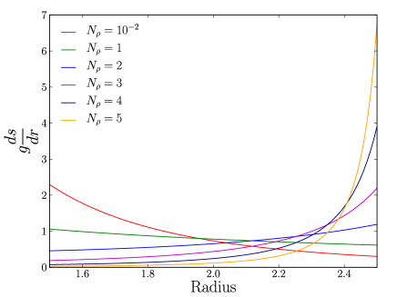
Figure 1: Radial profile of $g|ds_{c}/dr|$ for different background density stratifications $N_{\rho}=[10^{-2},1,2,3,4,5]$.

Several authors argued that Rayleigh numbers at mid-depth may offer a more meaningful reference value (e.g. Unno et al., 1960; Gough et al., 1976; Glatzmaier and Gilman, 1981). Here we follow Kaspi et al. (2009), who suggest to use a mass-weighted average defined as

$$\langle{\cal R}\rangle_{\rho}=\dfrac{d^{4}}{c_{p}\nu\kappa}\left\langle g\left|\dfrac{ds_{c}}{dr}\right|\right\rangle_{\rho},$$ (14)

where the average is defined as $\langle\cdots\rangle_{\rho}=\int_{r_{i}}^{r_{o}}(\cdots)\bar{\rho}r^{2}dr/\int_{r_{i}}^{r_{o}}\bar{\rho}r^{2}dr$ (Kaspi et al., 2009). This new definition of the Rayleigh number can be related to the usual one (Eq. 11), by the coefficient $\langle g|ds/dr|_{c}\rangle_{\rho}$, that has an analytical solution for a polytropic index of $2$

$$\left\langle g\left|\dfrac{ds_{c}}{dr}\right|\right\rangle_{\rho}=\dfrac{3N_{\rho}}{\left(1-e^{-N_{\rho}}\right)\left(1+\eta e^{N_{\rho}/2}+\eta^{2}e^{N_{\rho}}\right)}.$$ (15)

Moreover, in the limit of small viscosity and thermal diffusivity, the force balance is expected to become independent on viscosity (low Ekman number). Therefore, following Christensen (2002) and Christensen and Aubert (2006), it is more relevant to consider a modified Rayleigh number that does not depend anymore on diffusivities, defined as

$$\left\langle\text{Ra}^{*}\right\rangle_{\rho}=\dfrac{1}{c_{p}\Omega^{2}}\left\langle g\left|\dfrac{ds_{c}}{dr}\right|\right\rangle_{\rho}=\langle{\cal R}\rangle_{\rho}\,\text{E}^{2}\,\text{Pr}^{-1}.$$ (16)

To get a non-dimensional measure of the radial heat transport that is also independent of the thermal diffusivity, we use a modified Nusselt number

$$\text{Nu}^{*}=\dfrac{q}{\rho T\Omega d^{2}(ds_{c}/dr)}=\text{Nu}\,\text{E}\,\text{Pr}^{-1}.$$ (17)

where $q$ is the heat flux. Once the simulation has reached the nonlinear saturation, the time-average of this modified Nusselt number should become constant with radius as there is no internal heat source in the system. Therefore, there is no need to consider mass-weighted average of this parameter.

Finally, it is also useful to analyse our simulations in terms of an alternate Rayleigh number based on the heat flux rather than on the entropy contrast $\Delta s$

$$\hbox{Ra}_{q}^{*}=\dfrac{qg}{c_{p}\rho T\Omega^{3}d^{2}}.$$ (18)

This flux-based Rayleigh number can be related to the modified Nusselt number as follows

$$\hbox{Ra}_{q}^{*}=\dfrac{g}{c_{p}\Omega^{2}}\left|\dfrac{ds_{c}}{dr}\right|\text{Nu}^{*}=\text{Ra}^{*}\,\text{Nu}^{*}.$$ (19)

Once again, this number varies with radius, and therefore it is useful to consider the mass-weighted average counterpart of this quantity

$$\langle\hbox{Ra}_{q}^{*}\rangle_{\rho}=\left\langle\hbox{Ra}^{*}\right\rangle_{\rho}\,\text{Nu}^{*}.$$ (20)

2.2 The numerical method

The numerical simulations of this study have been carried out with a modified version of the code MagIC (Wicht, 2002). The new anelastic version has been tested and validated against different compressible convection and dynamo benchmarks (Jones et al., 2011). To solve the system of equations (4), (5) and (7) in spherical coordinates $(r,\theta,\phi)$, the mass flux $\bar{\rho}\mathchoice{\mbox{\boldmath$\displaystyle u$}}{\mbox{\boldmath$\textstyle u$}}{\mbox{\boldmath$\scriptstyle u$}}{\mbox{\boldmath$\scriptscriptstyle u$}}$ is decomposed into a poloidal and a toroidal contribution

$$\bar{\rho}\mathchoice{\mbox{\boldmath$\displaystyle u$}}{\mbox{\boldmath$\textstyle u$}}{\mbox{\boldmath$\scriptstyle u$}}{\mbox{\boldmath$\scriptscriptstyle u$}}=\mathchoice{\mbox{\boldmath$\displaystyle\nabla$}}{\mbox{\boldmath$\textstyle\nabla$}}{\mbox{\boldmath$\scriptstyle\nabla$}}{\mbox{\boldmath$\scriptscriptstyle\nabla$}}\times\left(\mathchoice{\mbox{\boldmath$\displaystyle\nabla$}}{\mbox{\boldmath$\textstyle\nabla$}}{\mbox{\boldmath$\scriptstyle\nabla$}}{\mbox{\boldmath$\scriptscriptstyle\nabla$}}\times W\mathchoice{\mbox{\boldmath$\displaystyle e_{r}$}}{\mbox{\boldmath$\textstyle e_{r}$}}{\mbox{\boldmath$\scriptstyle e_{r}$}}{\mbox{\boldmath$\scriptscriptstyle e_{r}$}}\right)+\mathchoice{\mbox{\boldmath$\displaystyle\nabla$}}{\mbox{\boldmath$\textstyle\nabla$}}{\mbox{\boldmath$\scriptstyle\nabla$}}{\mbox{\boldmath$\scriptscriptstyle\nabla$}}\times Z\mathchoice{\mbox{\boldmath$\displaystyle e_{r}$}}{\mbox{\boldmath$\textstyle e_{r}$}}{\mbox{\boldmath$\scriptstyle e_{r}$}}{\mbox{\boldmath$\scriptscriptstyle e_{r}$}},$$ (21)

where $W$ and $Z$ are the poloidal and toroidal potentials. $W$, $Z$, $p$ and $s$ are then expanded in spherical harmonic functions up to degree $\ell_{\text{max}}$ in the angular variables $\theta$ and $\phi$ and in Chebyshev polynomials up to degree $N_{r}$ in the radial direction. The equations for $W$ and $Z$ are obtained by taking the horizontal part of the divergence and the radial component of the curl of Eq. (5), respectively. A more exhaustive description of the numerical method and spectral transforms involved in the computation can be found in (Gilman and Glatzmaier, 1981) and in (Christensen and Wicht, 2007).

2.3 Boundary conditions

In all the simulations presented in this study, we have assumed constant entropy and stress-free boundary conditions for the velocity at both limits. Under the anelastic approximation, the non-penetrating stress-free boundary conditions is modified compared to the usual Boussinesq one as it now involves the background density

$$\dfrac{\partial}{\partial r}\left(\dfrac{1}{r^{2}\bar{\rho}}\dfrac{\partial W}{\partial r}\right)=\dfrac{\partial}{\partial r}\left(\dfrac{1}{r^{2}\bar{\rho}}Z\right)=0\quad\text{for}\quad r=[r_{i},r_{o}].$$ (22)

The non-penetrating condition of the radial motion is not affected by the anelastic approximation and remains $u_{r}=0$ (or $W=0$) at both limits.

3 Physical properties of compressible convection

We have fixed the aspect ratio $\eta=0.6$ to the lower value suggested for the molecular to metallic hydrogen transition in Jupiter ($0.85~{}R_{J}$) and Saturn ($0.6~{}R_{S}$) (e.g. Liu et al., 2008). This limits the numerical difficulties associated with thinner shells and therefore allows to reach higher density stratification. The Ekman number is kept fixed at $\text{E}=10^{-4}$, which is larger than the most extreme values chosen by Jones and Kuzanyan (2009) but allows us to conduct a large number of simulations. Following previous Boussinesq studies (e.g. Christensen, 2002), the Prandtl number is set to $1$, while the polytropic index is $m=2$ following Jones and Kuzanyan (2009). Being mostly interested in the effects of density stratification on zonal flow generation, we have performed simulations at five different values of $N_{\rho}$ $(10^{-2},1,2,3,4,5)$ that span the range from nearly Boussinesq to a density contrast of 150. In the gas giants, the density jump between the 1 bar level and the bottom of the molecular region corresponds to $N_{\rho}\simeq 8.5$ (e.g Guillot, 1999; Nettelmann et al., 2008). For numerical reasons, we cannot afford to increase $N_{\rho}$ beyond $5$. However, since the density gradient decreases rapidly with depth, $N_{\rho}=5$ covers already $99\%$ of the molecular envelope when starting at the metallic transition. The remaining rather thin upper atmosphere (roughly 500 kms) may involve additional physical effects such as radiative transfer, weather effects or insolation, that we do not include in our model. For each of the stratifications used in this study, the Rayleigh number has been varied, starting from close to onset up to 140 times the critical value. Altogether more than 140 simulations have been computed, each running for at least 0.2 viscous time ensuring that the nonlinear saturation has been reached (see Table 2).

The numerical resolution increases from $(N_{r}=73,\ \ell_{\text{max}}=85)$ for Boussinesq runs close to onset to $(N_{r}=161,\ \ell_{\text{max}}=341)$ for the more demanding highly supercritical simulations with strong stratification. In the latter cases, we have resolved to imposing a two-fold or a four-fold azimuthal symmetry, effectively solving for only half or a quarter of the spherical shell, respectively. A comparison of testruns with or without symmetries showed no significant statistical differences.

3.1 Onset of convection

Table 1: Values of the critical Rayleigh numbers (and flux-based counterparts) and azimuthal wavenumbers for different background density stratifications (with $\text{E}=10^{-4}$ and $\text{Pr}=1$).

$N_{\rho}$	$\text{Ra}_{\text{crit}}$	$\text{Ra}_{q}^{*}$	$\langle\text{Ra}_{q}^{*}\rangle_{\rho}$	$m_{\text{crit}}$
$10^{-2}$	$1.739\times 10^{5}$	$1.739\times 10^{-7}$	$2.666\times 10^{-7}$	21
1	$5.175\times 10^{5}$	$5.175\times 10^{-7}$	$8.275\times 10^{-7}$	34
2	$1.141\times 10^{6}$	$1.141\times 10^{-6}$	$1.496\times 10^{-6}$	53
3	$1.529\times 10^{6}$	$1.529\times 10^{-6}$	$1.326\times 10^{-6}$	72
4	$1.852\times 10^{6}$	$1.852\times 10^{-6}$	$9.023\times 10^{-7}$	83
5	$2.341\times 10^{6}$	$2.341\times 10^{-6}$	$5.727\times 10^{-7}$	93

Figure 2: Radial component of the velocity $u_{r}$ in the equatorial plane for different density stratifications very close to onset of convection (less than $5\%$ over the critical Rayleigh number). Outward flows are rendered in red, inward flows in blue, dimensionless radial velocities are expressed in terms of Reynolds numbers.

The linear stability analysis by Jones et al. (2009) shows that density stratification can have a significant influence both on the value of the critical Rayleigh number and on the location of the first unstable mode. To facilitate the comparison between different density contrasts, we have therefore computed the corresponding critical Rayleigh numbers (Tab. 1). The values have been obtained by trial and error, monitoring the growth or decay of initial disturbances at various Rayleigh numbers.

Figure 2 emphasises how the location of the convective instability changes when $N_{\rho}$ is increased. In the nearly Boussinesq case ($N_{\rho}=10^{-2}$), convection sets in near the tangent cylinder. The convective columns show a strong prograde spiralling, typical for rapidly rotating convection at a moderate Prandtl number (e.g. Zhang, 1992). For $N_{\rho}=1$, the wavenumber increases but the instability stays attached to the inner boundary. However, when increasing $N_{\rho}$ further, it moves outward and is progressively confined to the very thin outermost region.

This behaviour can be explained by the depth-dependent of buoyancy expressed via the modified Rayleigh number (Eq. 12). Figure 2 demonstrates how larger buoyancy values are more and more confined close to the outer boundary as $N_{\rho}$ grows. This implies a decrease in radial lengthscale, which goes along with a rapid increase in wavenumber. This allows the instability to maintain a more or less spherical cross section (Glatzmaier and Gilman, 1981; Jones et al., 2009).

3.2 Convection regimes

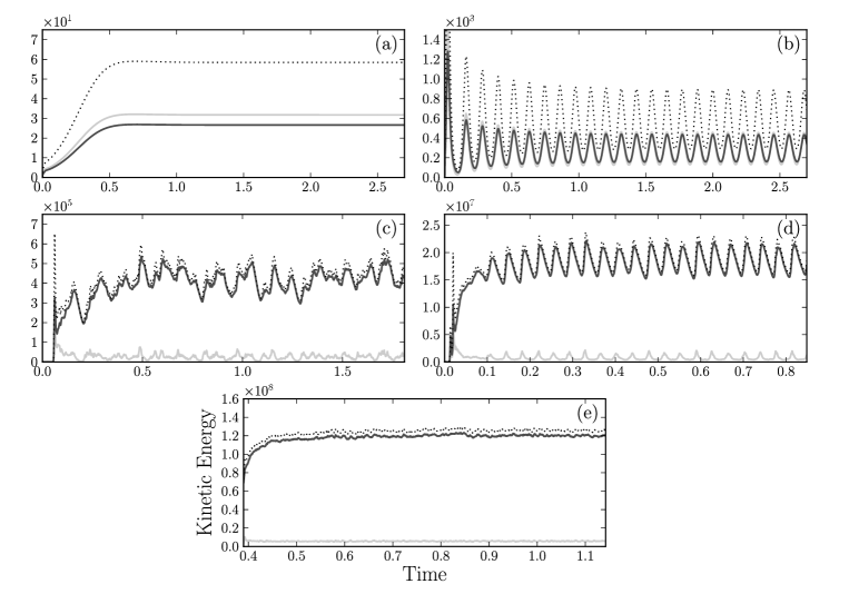
Figure 3: Time series of the kinetic energy for different simulations with a moderate density contrast ($N_{\rho}=2$). In each panel, the dotted black line corresponds to the total kinetic energy, while solid black line and solid gray line correspond respectively to toroidal an poloidal parts of the kinetic energy. The simulation displayed in (a) corresponds to $\text{Ra}=1.145\times 10^{6}$ ($1.004\times$ supercritical), (b) to $\text{Ra}=1.2\times 10^{6}$ ($1.05\times$ supercritical), (c) to $\text{Ra}=2.2\times 10^{6}$ ($1.93\times$ supercritical), (d) to $\text{Ra}=8\times 10^{6}$ ($7\times$ supercritical) and (e) to $\text{Ra}=2\times 10^{7}$ ($17.5\times$ supercritical). These five simulations can be localized in the regime diagram displayed in Fig. 4.

The properties of rotating thermal convection have been explored extensively under the Boussinesq approximation (e.g. Zhang, 1992; Grote and Busse, 2001; Christensen, 2001). The respective studies show that when the Rayleigh number is increased beyond onset distinct regimes with different temporal behavior are encountered. Here we explore whether these regimes are retained in the presence of density stratification.

Figure 3 illustrates the time dependence in the temporal variation characteristic for the different regimes at $N_{\rho}=2$ and in Fig. 4 we attempt to show how the regimes boundaries change on increasing $N_{\rho}$. At $N_{\rho}=2$, we still find the same regimes identified in the Boussinesq simulations. Very close to onset, the solutions simply drift in azimuth due to its Rossby wave character (Busse, 1994) and the kinetic energy becomes stationary (Fig. 3a). The drift is a consequence of both the height change of the container and the background density stratification encountered by the convective instability. Its amplitude and direction depends on the chosen stratification (Evonuk, 2008; Glatzmaier et al., 2009). At a still rather small supercriticality, the solution starts to vacillate in amplitude, while retaining its columnar form. Figure 3b demonstrates that the poloidal and toroidal kinetic energies oscillate in phase and have a comparable magnitude.

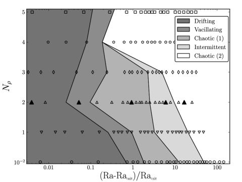
Figure 4: Regime diagram $(\text{Ra},N_{\rho})$ displaying how the different nonlinear regimes of rotating compressible convection depend on supercriticality and density stratification. Each symbol corresponds to one simulation computed in this study. The five black triangles denote the localisations of the five simulations emphasised in Fig. 3.

A further increase of the Rayleigh number leads to a third regime with a more chaotic time-dependence (Fig. 3c). The zonal flow production is already so efficient that the toroidal energy dominates the kinetic energy budget. Since the poloidal flow is directly driven by convective up- and downwellings, its amplitude can serve as a proxy for the convective flow vigor. Zonal flows are the axisymmetric contribution of toroidal flow and already dominate the toroidal energy here. Both the convective and the zonal flows display large amplitude modulations. A fourth regime with intermittent nearly oscillatory convection is encountered once $\text{Ra}\gtrsim 4\times\text{Ra}_{c}$ (panel (d) in Fig. 3). Here, the zonal flow periodically becomes so large that the associated shear disrupts the convective structures (see for further details Christensen, 2001; Grote and Busse, 2001; Simitev and Busse, 2003; Heimpel and Aurnou, 2012). The Reynolds stresses then decrease and the zonal flow cannot be maintained any more against viscous forces. The convection recovers once the zonal flows amplitude has decreased sufficiently. A similar but less regular competition may also cause the large variation in the chaotic regime. Typical for this intermittent regime, which has mainly been observed in Boussinesq simulations but has also been reported in some anelastic simulations of turbulent convection in solar-like stars (Ballot et al., 2007), is that the convective features typically occupy only an azimuthal fraction of the volume. Finally, in the strongly supercritical regime, convection becomes once more chaotic but the variations are much smaller than in the first chaotic regime (Fig. 3e). Convective features now fill the whole spherical shell and efficiently drive strong zonal winds.

For $N_{\rho}=2$ we thus find the following regime succession also typical for Boussinesq convection at $\text{Pr}\lesssim 1$ (Grote and Busse, 2001):

$$\text{Drifting}\rightarrow\text{Vacillating}\rightarrow\text{Chaotic}\rightarrow\text{Intermittent}\rightarrow\text{Chaotic}\;.$$

The regime diagram displayed in Fig. 4 shows that the first chaotic and the intermittent regime tend to vanish for larger values of $N_{\rho}$. For $N_{\rho}=[4-5]$, we found neither the first chaotic nor the intermittent regime, which could mean that both have retreated to a rather small region of the parameter space or are missing altogether. Due to the lack of an intermittent regime, however, the separation of the first and second chaotic regime is less clear cut, being based only on the variation amplitude. The narrowing of the regime diagram for increasing density stratification was also found in 3-D simulations of convection in rapidly rotating isothermal spherical shells (Tortorella, 2005).

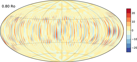
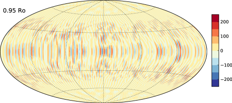
Figure 5: Radial velocity $u_{r}$ on spherical surfaces at three different radii close to the inner boundary ($r=0.65r_{o}$), at the layer middle, and close to the outer boundary ($r=0.95r_{o}$). Outward flows are rendered in red, inward flows in blue, dimensionless radial velocities are expressed in terms of Reynolds numbers. From a model with $N_{\rho}=5$ and $\text{Ra}=8\times 10^{6}$.

The large amplitude oscillations in the first chaotic and the intermittent regime require a more global interaction between convection and zonal flow. When the density stratification is increased, however, the solution becomes more small scale and chaotic and the convective columns progressively loose their integrity in the direction of the rotation axis (Glatzmaier et al., 2009; Jones and Kuzanyan, 2009). This likely prevents the required more global interaction and the related regimes at larger density stratification.

3.3 Flow properties

The background density stratification causes significant changes in the convective flow that we discuss first before describing the zonal flows in section 3.3.2.

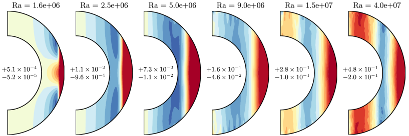
Figure 6: Zonally averaged azimuthal velocity in the meridian plane for simulations with $N_{\rho}=3$ and different Rayleigh numbers. Colorscales are centered around zero: prograde jets are rendered in red, retrograde jets in blue. Prograde contours have been truncated in amplitude to emphasize the structure of the retrograde flows. Dimensionless azimuthal velocities are expressed here in terms of Rossby numbers. The extrema of the zonal flow velocity are indicated in the center of each panel.

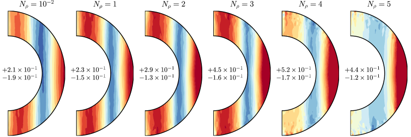
Figure 7: Zonally averaged azimuthal velocity in the meridian plane for simulations with different density stratifications. The different setups correspond to $N_{\rho}=10^{-2}$, $\langle\text{Ra}_{q}^{*}\rangle_{\rho}=1.70\times 10^{-4}$ (i.e. $\text{Ra}=1.2\times 10^{7}$); $N_{\rho}=1$, $\langle\text{Ra}_{q}^{*}\rangle_{\rho}=1.50\times 10^{-4}$ (i.e. $\text{Ra}=1.2\times 10^{7}$); $N_{\rho}=2$, $\langle\text{Ra}_{q}^{*}\rangle_{\rho}=1.37\times 10^{-4}$ (i.e. $\text{Ra}=1.5\times 10^{7}$); $N_{\rho}=3$, $\langle\text{Ra}_{q}^{*}\rangle_{\rho}=2.63\times 10^{-4}$ (i.e. $\text{Ra}=3.2\times 10^{7}$);$N_{\rho}=4$, $\langle\text{Ra}_{q}^{*}\rangle_{\rho}=2.84\times 10^{-4}$ (i.e. $\text{Ra}=6\times 10^{7}$) and $N_{\rho}=5$, $\langle\text{Ra}_{q}^{*}\rangle_{\rho}=1.48\times 10^{-4}$ (i.e. $\text{Ra}=7.5\times 10^{7}$) . Colorscales are centered around zero: prograde jets are rendered in red, retrograde jets in blue. Prograde contours have been truncated in amplitude to emphasize the structure of the retrograde flows. Dimensionless azimuthal velocities are expressed here in terms of Rossby numbers. The extrema of the zonal flow velocity are indicated in the center of each panel.

3.3.1 Convective flows

Figure 5 illustrates how the radial velocity varies with depth in a strongly-stratified anelastic simulation at $N_{\rho}=5$. The Rayleigh number of $\text{Ra}=8\times 10^{6}$ guarantees that the solution is safely located in the second chaotic regime. Deeper within the interior, the convection is characterized by larger azimuthal length scales and lower amplitudes. With increasing radius, the azimuthal length scale decreases, while the amplitude increases. The convective features remain roughly aligned with the rotation axis at any radius. The changes in length scale are coupled to the background density profile as the density scale height defined by $H_{\rho}=-(d\ln\bar{\rho}/dr)^{-1}$ is a good proxy for the typical size of the convective eddies. At $N_{\rho}=5$, this scale height decreases by a factor of five when going from the inner to the outer boundary, which about explains the variation shown in Fig. 5.

The increase in amplitude can be explained by the variation of the background density: since $\bar{\rho}$ decreases by a factor of about $150$ from $r_{i}$ to $r_{o}$, a rising (falling) convective plume compensates this with increasing (decreasing) flow amplitude. Figure 5 shows an increase of about 60 which seems somewhat on the low side. However, the radial increase in the number of convective columns and the scale change show that the convective features hardly reach through the whole shell without being modified.

3.3.2 Zonal flows

Evonuk (2008) and Glatzmaier et al. (2009) argue that the density stratification can significantly influence the generation of zonal winds. Exploring the possible related effects is the main focus of our study. Figure 6 shows how the zonal flows evolve on increasing the Rayleigh number in moderately stratified simulations ($N_{\rho}=3$). Close to the onset of convection, a thin prograde equatorial jet develops in the very outer part of the shell. The latitudinal extent of this jet is smaller than in Boussinesq convection because the convective columns are confined closer to the outer boundary (see the simulation with $N_{\rho}=3$ in Fig. 2). It is flanked by weak amplitude retrograde jets that strongly vary along $z$. As Ra is increased, convection starts to fill the whole shell, the equatorial jet broadens and the zonal winds become more and more geostrophic with a second retrograde jet that reaches throughout the shell. For $\text{Ra}=5\times 10^{6}$ ($3.3\times$ critical) the equatorial jet has reached a maximum width that it retains at even higher Rayleigh numbers. The retrograde jet broadens toward higher latitudes until additional flanking prograde jets develop below and above the inner boundary at large Rayleigh numbers and confine it to mid latitudes. The amplitude of these high-latitude jets becomes comparable to that of the equatorial jet for strongly nonlinear simulations ($\text{Ra}=4\times 10^{7}$, $26\times\text{Ra}_{c}$), while the retrograde jet vigor intensifies to about 50% of this amplitude. In this multiple jets regime, retrograde zonal winds are anchored to the tangent cylinder in a similar way to what was already observed in Boussinesq simulations (e.g. Christensen, 2001; Heimpel et al., 2005).

The strong $z$-dependence at low Rayleigh numbers is a typical thermal wind feature, which can be understood by considering the $\phi$-component of the curl of the momentum equation (5):

$$\dfrac{D\omega_{\phi}}{Dt} = r\sin\theta\ (\mathchoice{\mbox{\boldmath$\displaystyle\omega$}}{\mbox{\boldmath$\textstyle\omega$}}{\mbox{\boldmath$\scriptstyle\omega$}}{\mbox{\boldmath$\scriptscriptstyle\omega$}}\cdot\mathchoice{\mbox{\boldmath$\displaystyle\nabla$}}{\mbox{\boldmath$\textstyle\nabla$}}{\mbox{\boldmath$\scriptstyle\nabla$}}{\mbox{\boldmath$\scriptscriptstyle\nabla$}})\left(\dfrac{u_{\phi}}{r\sin\theta}\right)-\omega_{\phi}\mathchoice{\mbox{\boldmath$\displaystyle\nabla$}}{\mbox{\boldmath$\textstyle\nabla$}}{\mbox{\boldmath$\scriptstyle\nabla$}}{\mbox{\boldmath$\scriptscriptstyle\nabla$}}\cdot\mathchoice{\mbox{\boldmath$\displaystyle u$}}{\mbox{\boldmath$\textstyle u$}}{\mbox{\boldmath$\scriptstyle u$}}{\mbox{\boldmath$\scriptscriptstyle u$}}+\dfrac{2}{\text{E}}\dfrac{\partial u_{\phi}}{\partial z}$$ (23)

$$-\dfrac{\text{Ra}}{\text{Pr}}\dfrac{r_{o}^{2}}{r^{3}}\dfrac{\partial s}{\partial\theta}+\left[\mathchoice{\mbox{\boldmath$\displaystyle\nabla$}}{\mbox{\boldmath$\textstyle\nabla$}}{\mbox{\boldmath$\scriptstyle\nabla$}}{\mbox{\boldmath$\scriptscriptstyle\nabla$}}\times\left(\bar{\rho}^{-1}\mathchoice{\mbox{\boldmath$\displaystyle\nabla$}}{\mbox{\boldmath$\textstyle\nabla$}}{\mbox{\boldmath$\scriptstyle\nabla$}}{\mbox{\boldmath$\scriptscriptstyle\nabla$}}\cdot\mathsf{S}\right)\right]_{\phi}.$$

Here $D/Dt$ corresponds to the substantial time derivative and $\omega_{\phi}$ is the azimuthal vorticity component. For low Rayleigh numbers, inertial contributions can be neglected, and the $z$-dependence of the zonal flows is ruled by the thermal wind balance:

$$\dfrac{2}{\text{E}}\dfrac{\partial\overline{u_{\phi}}}{\partial z}\simeq\dfrac{\text{Ra}}{\text{Pr}}\dfrac{r_{o}^{2}}{r^{3}}\dfrac{\partial\overline{s}}{\partial\theta},$$ (24)

where overlines denote an azimuthal average. This allows us to define the typical lengthscale

$$L_{z}=\left(\dfrac{\partial\ln\overline{u_{\phi}}}{\partial z}\right)^{-1}=\overline{u_{\phi}}\ \left(\dfrac{\text{Ra}\ \text{E}}{2\text{Pr}}\dfrac{r_{o}^{2}}{r^{3}}\dfrac{\partial\overline{s}}{\partial\theta}\right)^{-1}.$$ (25)

For vanishing Ekman numbers, $L_{z}$ approaches infinity and zonal flows become independent of $z$, recovering Taylor-Proudman theorem and therefore a geostrophic structure. For the lowest Rayleigh number solution shown in Fig. 6a, the thermal winds caused $z$-variation is still clearly apparent where $u_{\phi}$ is weak and $L_{z}$ therefore small. At larger Rayleigh numbers, the thermal wind balance still holds in a statistical sense. According to Eq. (24), $\partial\overline{u_{\phi}}/\partial z$ increases linearly with Ra, while, at least closer to onset, the zonal flow amplitude rises faster. $L_{z}$ therefore grows with the Rayleigh number and the $z$-variation is gradually lost. In the simulations of Kaspi et al. (2009) however, the zonal winds still vary strongly close to the surface. These are likely promoted by the depth-dependence of the thermal expansion coefficient, which is neglected in our ideal gas model.

Figure 7 compares the zonal flows at different density stratifications for simulations with similar $\langle\text{Ra}_{q}^{*}\rangle_{\rho}$ and demonstrates that the structure changes very little for $N_{\rho}\leq 3$. In the two cases at $N_{\rho}=4$ and $N_{\rho}=5$ the high-latitude jets are still little pronounced and the retrograde jet is also rather weak. According to the development shown in Fig. 6 they seem to correspond to a lower supercriticality. The fact that $N_{\rho}=4$ and $5$ simulations have a supercriticality that is about three times higher than that of the $N_{\rho}=2$ case, however, implies that significantly larger supercriticalities are required to reach a comparable multiple jet structure when the density stratification is strong. Since both large Rayleigh numbers and strong density stratifications promote smaller scales, we could not afford to further increase Ra for $N_{\rho}>3$. While the zonal winds are very geostrophic for smaller density stratification, additional non-geostrophic small scale features start to appear for larger stratifications as it has already been reported by Jones and Kuzanyan (2009). They are strongly time-dependent and therefore disappear when time averaged quantities are considered.

Except for these secondary features and the requirement for larger supercriticalities at stronger stratifications, the zonal flow structure is surprisingly independent of the background density profile. We now turn to discussing their amplitude.

4 Scaling laws

To evaluate how the different flow properties depend on the background density stratification, we consider time averaged quantities in the following. Each simulation has been run for at least $0.2$ viscous diffusions times to get rid of any transients and to allow for an averaging period long enough to suppress short term variations. The Reynolds numbers Re and Rossby numbers $\text{Ro}=\text{E}\ \text{Re}$, used to quantify the amplitude of different flow contributions are based on the non-dimensional time averaged root-mean square velocity:

$$\text{Re}=\left(\langle u^{2}\rangle\right)^{1/2},$$ (26)

with

$$\langle u^{2}\rangle=\dfrac{1}{\tau}\dfrac{1}{V_{s}}\int_{t_{0}}^{t_{0}+\tau}\int_{V}\mathchoice{\mbox{\boldmath$\displaystyle u$}}{\mbox{\boldmath$\textstyle u$}}{\mbox{\boldmath$\scriptstyle u$}}{\mbox{\boldmath$\scriptscriptstyle u$}}^{2}dt\ dV,$$ (27)

where $\tau$ is the averaging interval, $V_{s}$ is the volume of the spherical shell and $dV$ is a volume element. As pointed out by Kaspi et al. (2009), a comparison of simulations with different density backgrounds may be more relevant if one considers mass-weighted average quantities. Therefore, the mass-weighted counterparts of Reynolds and Rossby numbers are defined using the time averaged kinetic energy, that is

$$\langle\text{Re}\rangle_{\rho}=\left(\frac{2E_{\text{kin}}}{\langle\bar{\rho}\rangle}\right)^{1/2},$$ (28)

with

$$E_{\text{kin}}=\dfrac{1}{\tau}\dfrac{1}{V_{s}}\int_{t_{0}}^{t_{0}+\tau}\int_{V}\bar{\rho}\mathchoice{\mbox{\boldmath$\displaystyle u$}}{\mbox{\boldmath$\textstyle u$}}{\mbox{\boldmath$\scriptstyle u$}}{\mbox{\boldmath$\scriptscriptstyle u$}}^{2}dt\ dV.$$ (29)

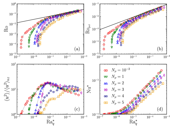
Figure 8: Time-averaged properties plotted against flux-based Rayleigh number defined in Eq. (19): (a) Rossby number; (b) Rossby number for the poloidal flow component; (c) ratio of square velocity over non-zonal square velocity; (d) modified Nusselt number.

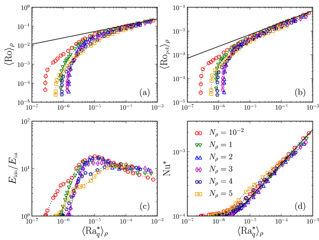
Figure 9: Time-averaged properties plotted against mass-weighted flux-based Rayleigh number defined in Eq. (20): (a) mass-weighted Rossby number; (b) mass-weighted Rossby number for the poloidal flow component; (c) ratio of kinetic energy over non-zonal kinetic energy; (d) modified Nusselt number.

Figures 8 and 9 show how different time-average properties for the various density stratifications explored here depend on the flux-based Rayleigh number (Eq. 19) and the mass-weighted flux-based Rayleigh number (Eq. 20), respectively. The total Rossby number Ro (Fig. 8a) and the poloidal Rossby number $\text{Ro}_{\text{pol}}$ (Fig. 8b), as well as their mass-weighted counterparts (Fig. 9a-b) first rise steeply. The slope flattens once convection fills the whole shell and seems to reach an asymptotic value for large Rayleigh numbers. The asymptotic slopes are larger for the poloidal than for the total flow amplitude. In both Figs. 8 and 9, the curves collapse at larger Rayleigh numbers, and the asymptotic slopes become independent of the density stratification. This is even more convincing when mass-weighted average quantities are considered, which basically confirms Kaspi et al. (2009). The remaining differences at low Rayleigh numbers can at least partly be explained by the different critical values. Compared to the gas giants, the Rossby numbers where our simulations reach the asymptotic regime are roughly one order of magnitude larger. However this is likely a consequence of the moderate Ekman number used in our models as Christensen (2002) showed that this transitional Rossby number decreases with Ekman number.

Figure 9c displays the ratio of the total to the non-zonal kinetic energy, while Fig. 8c corresponds to the ratio of square velocities only. For all density stratifications, this ratio initially increases in the weakly supercritical regime but decays once the convection becomes strongly nonlinear. Similarly to what has been reported for Boussinesq simulations (Christensen, 2002), the maximum is reached close to the transition to the intermittent regime (see Fig. 4 for $N_{\rho}\leq 3$).

In the nearly Boussinesq simulations, the maximum ratio is $E_{\text{kin}}/E_{\text{nz}}\simeq 20$, which means that $95$% of the energy are carried by zonal flows. For $N_{\rho}=5$ this decreases to about $90$% at a maximum ratio of $E_{\text{kin}}/E_{\text{nz}}\simeq 10$. These values are on the low side of the expected ratio for Jupiter: around $50-100$ from the work of Salyk et al. (2006). However, this moderate maximum ratio is once more a consequence of the too large Ekman number used in our simulations (Christensen, 2002). The slope of the decrease for larger Rayleigh numbers also seems to vary with $N_{\rho}$, but a clear dependence is difficult to extract from our dataset. Considering mass-weighted quantities slightly helps to merge the different simulations, but they are far from collapsing as nicely as for the Rossby numbers.

Panels (d) in Figs. 8 and 9 show the dependence of the modified Nusselt number on the Rayleigh numbers. Close to onset of convection, the heat transport is dominated by conduction. The classically defined Nusselt number remains close to unity and the Nusselt number increases only weakly with the Rayleigh number. When the convective motions become more vigorous, convective heat transport starts to dominate and the Nusselt number rises steeply. Using the mass-weighted Rayleigh number $\langle\text{Ra}_{q}^{*}\rangle_{\rho}$ allows to collapse the curves for different density stratifications and a similar asymptotic slope is reached. This once more emphasises that mass-weighted quantities are probably more meaningful parameters, when considering strongly nonlinear convection.

Based on the results displayed in Fig. 9 we have estimated the asymptotic dependence of $\langle\text{Ro}\rangle_{\rho}$, $\langle\text{Ro}_{\text{pol}}\rangle_{\rho}$ and $\text{Nu}^{*}$ on $\langle\text{Ra}_{q}^{*}\rangle_{\rho}$ to:

$$\langle\text{Ro}\rangle_{\rho}=2.45\left(\langle\hbox{Ra}_{q}^{*}\rangle_{\rho}\right)^{1/3},$$ (30)

$$\langle\text{Ro}_{\text{pol}}\rangle_{\rho}=2.25\left(\langle\hbox{Ra}_{q}^{*}\rangle_{\rho}\right)^{1/2},$$ (31)

$$\text{Nu}^{*}=0.086\left(\langle\hbox{Ra}_{q}^{*}\rangle_{\rho}\right)^{0.53}.$$ (32)

Black lines in Fig. 9 show the respective asymptotes. The same slopes have been obtained for the usual Rossby and poloidal Rossby numbers in Fig. 8, as the nearly Boussinesq simulations hardly depend on the density background (therefore mass-weighted counterparts of Rossby and poloidal Rossby numbers are equivalent to their usual definitions).

The amplitude of the convective flow, quantified via the poloidal Rossby number, is thus found to depend on the mass-weighted flux-based Rayleigh number with a slope of $1/2$. This is compatible with both laboratory experiments of turbulent rotating convection (e.g. Fernando et al., 1991) and previous anelastic numerical simulations (Showman et al., 2011) but slightly differs from the exponent $2/5$ suggested by Christensen (2002). Investigating the reason for this difference would probably require more simulations at lower Ekman numbers and lies beyond the scope of this study.

The Nusselt number scaling Eq. (32) is in a very good agreement with previous laws derived by Christensen (2002) and Christensen and Aubert (2006) for Boussinesq simulations. In the highly supercritical regime, the convective transport dominates diffusion. Then $\text{Nu}\sim u_{\text{conv}}\ \delta s$, or $\text{Nu}^{*}\sim\text{Ro}_{\text{pol}}\ \delta s$ where $\delta s$ is a measure for the typical entropy fluctuations. Since $\text{Nu}^{*}$ and $\text{Ro}_{\text{pol}}$ depend with a very similar exponent on $\langle\text{Ra}_{q}^{*}\rangle_{\rho}$, the typical entropy fluctuations $\delta s$ may vary very little with $\langle\text{Ra}_{q}^{*}\rangle_{\rho}$ in the asymptotic regime, in agreement with previous Boussinesq results (Christensen, 2002).

In the highly supercritical regime, the majority of the kinetic energy is carried by zonal flows. The asymptotic law for the total Rossby number (Eq. 30) therefore applies to the amplitude of zonal winds. Based on energy considerations for the highly supercritical regime, Showman et al. (2011) derived a scaling law for strong zonal jets that suggest an exponent of $1/2$ rather than the $1/3$ promoted here. We further discuss this difference in the following section.

4.1 Force balance and correlation of the convective flow

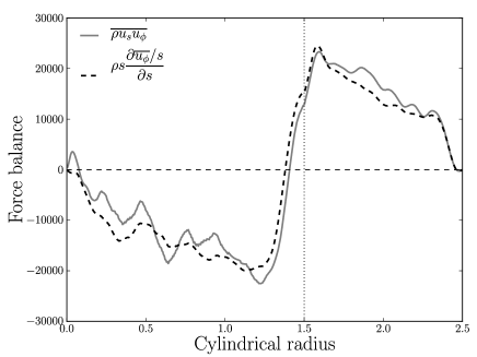
Figure 10: Time average of Reynolds stresses (solid grey line) and viscous force (dashed black line) integrated over cylinders (Eq. 34) for a model with $N_{\rho}=3$ and $\text{Ra}=2\times 10^{7}$. The vertical line corresponds to the tangent cylinder.

To explore how the strong zonal flows are generated and maintained, we analyze the azimuthal component of the Navier-Stokes equation (5) integrated over cylindrical surfaces of radius $s$. The Coriolis term is proportional to the net mass flux across these surfaces and therefore vanishes. The integrated Navier-Stokes equation thus simplifies to

$$\int_{S}\bar{\rho}\dfrac{\partial u_{\phi}}{\partial t}sd\phi dz= -\int_{S}\dfrac{1}{s^{2}}\dfrac{\partial}{\partial s}\left[s^{2}\bar{\rho}u_{s}u_{\phi}\right]sd\phi dz$$ (33)

$$+\int_{S}\dfrac{1}{s^{2}}\dfrac{\partial}{\partial s}\left[s^{2}\bar{\rho}s\dfrac{\partial}{\partial s}\left(\dfrac{u_{\phi}}{s}\right)\right]sd\phi dz.$$

On time average the two terms on the right hand side, Reynolds stress and viscous stress, should balance. This leads to the following condition

$$\int_{z}\bar{\rho}s\dfrac{\partial}{\partial s}\left(\dfrac{\overline{{u}_{\phi}}}{s}\right)dz=\int_{z}\overline{\bar{\rho}u_{s}u_{\phi}}dz,$$ (34)

where the overlines indicate an azimuthal average. Figure 10 compares the left and right hand side of Eq. (34) for a case with $N_{\rho}=3$ and $\text{Ra}=2\times 10^{7}$ (corresponding to $\langle Ra_{q}^{*}\rangle_{\rho}=1.7\times 10^{-4}$) that lies very close to the asymptotic regimes found in Fig. 9. These two terms balance to a good degree, which proves that zonal flows are indeed maintained by Reynolds stresses against viscous dissipation.

According to Eq. (10), we can also directly relate the viscous contribution in Fig. 9 to zonal flow gradients. Zonal flows are thus expected to increase outside the tangent cylinder, located at $s=1.5$, and to mainly decrease inside the tangent cylinder. A conversion to Reynolds stresses suggests that the strongest stresses can be found around the tangent cylinder and close to the outer boundary. The stresses are negative around the tangent cylinder and predominantly positive elsewhere. All this corresponds nicely to the multiple jet cases described above with a prograde equatorial jet, a retrograde jet around the tangent cylinder, and a prograde, high latitude jet in each hemisphere.

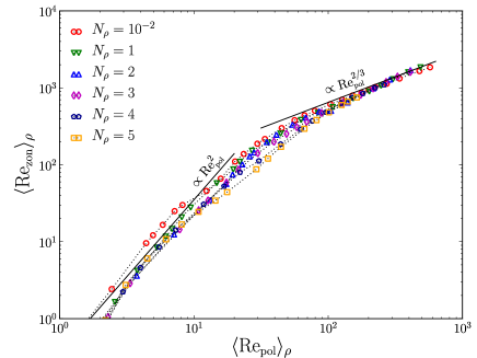
Figure 11: Reynolds number of axisymmetric zonal flows plotted against poloidal Reynolds number.

Since the typical length scale of the zonal jets remains of order unity, Eq. (10) suggests the scaling (e.g. Christensen, 2002)

$$\langle\text{Re}_{\text{zon}}\rangle_{\rho}\sim C_{s\phi}\ \langle\text{Re}_{\text{pol}}\rangle_{\rho}^{2},$$ (35)

where $\langle\text{Re}_{\text{zon}}\rangle_{\rho}$ is the Reynolds number of axisymmetric zonal flows and $C_{s\phi}$ quantifies the correlation of $u_{s}$ and $u_{\phi}$ throughout the shell:

$$C_{s\phi}=\dfrac{\left[\ \overline{\bar{\rho}u_{s}u_{\phi}}\ \right]}{\left[\left(\overline{\bar{\rho}u_{s}^{2}}\ \overline{\bar{\rho}u_{\phi}^{2}}\right)^{1/2}\right]}\;\;.$$ (36)

Here, the rectangular brackets $[\cdots]$ corresponds to an average over $s$ and $z$. In Fig. 11 we show $\langle\text{Re}_{\text{zon}}\rangle_{\rho}$ versus $\langle\text{Re}_{\text{pol}}\rangle_{\rho}$ for all the simulations of this study, while Fig. 12 shows the dependence of $C_{s\phi}$ on the mass-weighted flux-based Rayleigh number for some snapshots.

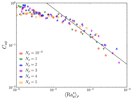
Figure 12: Correlation $C_{s\phi}$ plotted against mass-averaged flux-based Rayleigh number. The solid line is proportional to $\langle\text{Ra}_{q}^{*}\rangle_{\rho}^{-2/3}$.

For lower Rayleigh numbers and thus smaller poloidal Reynolds numbers $\langle\text{Re}_{\text{zon}}\rangle_{\rho}$ scales roughly like $\langle\text{Re}_{\text{pol}}\rangle_{\rho}^{2}$ and $C_{s\phi}$ is largely independent of the Rayleigh number. Convection assumes the form of regular large scale columns that are tilted in prograde direction due to the height change in the container and the background density stratification (e.g. Busse, 1983, 2002). The integrity of the rolls in z-direction and the consistent tilt guarantees a good correlation of $u_{s}$ and $u_{\phi}$ and $C_{s\phi}$ is of order one.

For larger Rayleigh numbers the results approach the asymptotic scaling

$$\langle\text{Re}_{\text{zon}}\rangle_{\rho}\sim\langle\text{Re}_{\text{pol}}\rangle_{\rho}^{2/3}.$$ (37)

When using Eq. (30) and Eq. (35) this suggests that

$$C_{s\phi}\sim\langle\text{Ra}_{q}^{*}\rangle_{\rho}^{-2/3},$$ (38)

which is more or less confirmed by the correlation shown in Fig. 12. The small scale turbulent motions that develop for highly supercritical convection tend to destroy the correlation (Christensen, 2002; Showman et al., 2011). Once more, neither the ratio of $\langle\text{Re}_{\text{zon}}\rangle_{\rho}$ to $\langle\text{Re}_{\text{pol}}\rangle_{\rho}$, nor the dependence of the correlation $C_{s\phi}$ on $\langle\text{Ra}_{q}^{*}\rangle_{\rho}$ is significantly affected by the different density stratifications employed.

The loss of correlation explains why the ratio of total to non-zonal kinetic energy shown in Fig. 9c decreases for larger Rayleigh numbers. Our scaling of $C_{s\phi}$ differs from Showman et al. (2011), who suggest an exponent of $-1/2$. This also explains the difference in the scaling of the Rossby number mentioned above. This difference may come from specific assumptions used in the model by (Kaspi et al., 2009). While these authors employ a more realistic equation of state, they also consider a simplified expression of the viscosity and neglect viscous heating. As Jones and Kuzanyan (2009) have demonstrated, viscous heating can contribute up to $50\%$ to the heat budget, and is therefore likely to influence the average flow properties in the strongly nonlinear regime.

4.2 Density stratification and vorticity production

The $z$-component of the vorticity equation allows to analyze how the correlation between $u_{s}$ and $u_{\phi}$ comes about. Taking the $z$-component of the curl of the momentum equation (5) leads to

$$\dfrac{D\omega_{z}}{Dt}-\left(\mathchoice{\mbox{\boldmath$\displaystyle\omega$}}{\mbox{\boldmath$\textstyle\omega$}}{\mbox{\boldmath$\scriptstyle\omega$}}{\mbox{\boldmath$\scriptscriptstyle\omega$}}\cdot\mathchoice{\mbox{\boldmath$\displaystyle\nabla$}}{\mbox{\boldmath$\textstyle\nabla$}}{\mbox{\boldmath$\scriptstyle\nabla$}}{\mbox{\boldmath$\scriptscriptstyle\nabla$}}\right)u_{z}= \dfrac{2}{\text{E}}\dfrac{\partial u_{z}}{\partial z}-\left(\dfrac{2}{\text{E}}+\omega_{z}\right)\mathchoice{\mbox{\boldmath$\displaystyle\nabla$}}{\mbox{\boldmath$\textstyle\nabla$}}{\mbox{\boldmath$\scriptstyle\nabla$}}{\mbox{\boldmath$\scriptscriptstyle\nabla$}}\cdot\mathchoice{\mbox{\boldmath$\displaystyle u$}}{\mbox{\boldmath$\textstyle u$}}{\mbox{\boldmath$\scriptstyle u$}}{\mbox{\boldmath$\scriptscriptstyle u$}}$$ (39)

$$-\dfrac{\text{Ra}}{\text{Pr}}\dfrac{r_{o}^{2}}{r^{3}}\dfrac{\partial s}{\partial\phi}+\left[\mathchoice{\mbox{\boldmath$\displaystyle\nabla$}}{\mbox{\boldmath$\textstyle\nabla$}}{\mbox{\boldmath$\scriptstyle\nabla$}}{\mbox{\boldmath$\scriptscriptstyle\nabla$}}\times\left(\bar{\rho}^{-1}\mathchoice{\mbox{\boldmath$\displaystyle\nabla$}}{\mbox{\boldmath$\textstyle\nabla$}}{\mbox{\boldmath$\scriptstyle\nabla$}}{\mbox{\boldmath$\scriptscriptstyle\nabla$}}\cdot\mathsf{S}\right)\right]_{z},$$

where $D/Dt$ denotes the substantial time derivative and $\omega_{z}$ is the vorticity component along the axis of rotation. For small Ekman numbers, the first two terms on the right hand side dominate. In the Boussinesq approximation, the divergence of $\textstyle u$ vanishes and thus only the first term can contribute. This is called the vortex stretching term because it describes the vorticity changes in a fluid column experiencing the height gradient of the container (e.g. Schaeffer and Cardin, 2005; Glatzmaier et al., 2009). Because of the curved boundary, the absolute value of the gradient and thus the stretching effect increases with $s$, leading to the prograde tilt of the convective columns (e.g. Busse, 1983, 2002). At larger Rayleigh numbers, these columns loose their integrity along $z$ and turbulent effects rather than the boundary curvature start to influence the flow. As reported above, this leads to the decrease in the correlation $C_{s\phi}$.

Besides this classical mechanism, compressibility brings a new vorticity source. As explained by Evonuk (2008) and Glatzmaier et al. (2009), rising (sinking) plumes generate negative (positive) vorticity due to the compressional source $(2\text{E}^{-1}+\omega_{z})\mathchoice{\mbox{\boldmath$\displaystyle\nabla$}}{\mbox{\boldmath$\textstyle\nabla$}}{\mbox{\boldmath$\scriptstyle\nabla$}}{\mbox{\boldmath$\scriptscriptstyle\nabla$}}\cdot\mathchoice{\mbox{\boldmath$\displaystyle u$}}{\mbox{\boldmath$\textstyle u$}}{\mbox{\boldmath$\scriptstyle u$}}{\mbox{\boldmath$\scriptscriptstyle u$}}$ in Eq. (39). In the 2-D anelastic simulations performed by Glatzmaier et al. (2009), the classical vortex stretching term is neglected and the new compressional term is the only source of vorticity. They report that the direction of the equatorial jet depends on the variations of the density background. According to Eq. (4), this new compressional source $\mathchoice{\mbox{\boldmath$\displaystyle\nabla$}}{\mbox{\boldmath$\textstyle\nabla$}}{\mbox{\boldmath$\scriptstyle\nabla$}}{\mbox{\boldmath$\scriptscriptstyle\nabla$}}\cdot\mathchoice{\mbox{\boldmath$\displaystyle u$}}{\mbox{\boldmath$\textstyle u$}}{\mbox{\boldmath$\scriptstyle u$}}{\mbox{\boldmath$\scriptscriptstyle u$}}=-(d\ln\bar{\rho}/dr)\ u_{r}$ is directly proportional to the density gradient. It is therefore expected to prevail closer to the outer boundary, where this gradient is strong. Moreover, since this mechanism is a local process, it may be less sensitive to the loss of correlation along a convective column with increasing Rayleigh number (Glatzmaier et al., 2009).

At first sight, however, this is hard to reconcile with the fact that the zonal wind structure depends little on the density stratification in our simulations. Figures 11 and 12 have actually demonstrated that the decorrelation affects all our cases to a similar degree, independently of the density background.

Figure 13: Time-average of the correlation $C_{s\phi}$ integrated over cylindrical surfaces for simulations with $N_{\rho}=10^{-2}$ (upper panel): $\text{Ra}=3\times 10^{6}$ (solid light-grey line), $\text{Ra}=5\times 10^{6}$ (dashed grey line), $\text{Ra}=8\times 10^{6}$ (dotted dark-grey line) and $\text{Ra}=1.5\times 10^{7}$ (dot-dashed black line); and for simulations with $N_{\rho}=5$ (lower panel): $\text{Ra}=1\times 10^{7}$ (solid light-grey line), $\text{Ra}=1.8\times 10^{7}$ (dashed grey line), $\text{Ra}=4\times 10^{7}$ (dotted dark-grey line) and $\text{Ra}=6\times 10^{7}$ (dot-dashed black line). The vertical line corresponds to the tangent cylinder.

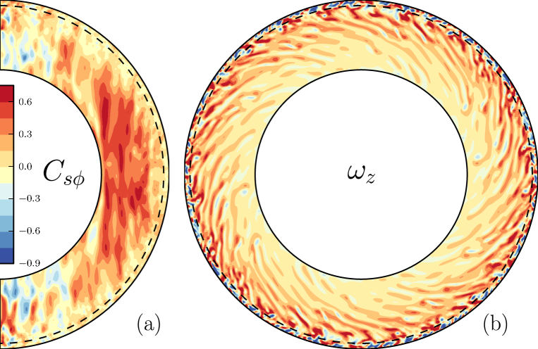
Figure 14: a) Correlation $C_{s\phi}$ in the meridian plane. b) Vorticity along the axis of rotation $\omega_{z}$ displayed in the equatorial plane. From a model with $N_{\rho}=5$, $\text{Ra}=4\times 10^{7}$. Positive values are rendered in red, negative ones in blue. The dashed lines in both panels correspond to the radius where the turnover timescale of convection becomes equal to the timescale associated with zonal shear (see Eq. 40).

In order to better understand the decorrelation, Fig. 13 compares the radial correlation profiles for nearly Boussinesq and $N_{\rho}=5$ cases at various Rayleigh numbers. In the nearly Boussinesq cases, the correlation is predominantly lost in the interior but changes very little close to the outer surface, in agreement with the results of Christensen (2002). For the strongly stratified cases, the correlation indeed peaks close to the outer boundary as expected from the new compressional vorticity source, as long as the Rayleigh number remains moderate. However, on increasing the supercriticality, this particularly strong correlation is lost first and the maximum of $C_{s\phi}$ is now located deeper in the interior.

This is also illustrated by Fig. 14a, which shows a meridional cut of azimuthally averaged $C_{s\phi}$. Figure 14b shows that the decorrelation goes along with a change in the vorticity pattern. In the inner part, the flow still shows a pronounced tilt that leads to Reynolds stresses and is clearly dominated by positive $z$-vorticity. Close to the outer boundary, convective motions are more radially oriented, without a preferred tilt or a clearly preferred sign. We attribute this to an increased mixing efficiency in the very outer part of the flow (Aurnou et al., 2007). The local turnover timescale of convection is a good proxy to quantify the mixing efficiency. We estimate this timescale to be $\tau_{\text{to}}\sim H_{\rho}/u_{\text{conv}}$. This can be compared with a timescale associated to zonal shear, defined by $\tau_{\text{zf}}\sim\delta/u_{\text{zonal}}$ (where $\delta$ is the typical width of the jets). To yield a significant correlation between $u_{s}$ and $u_{\phi}$, the shear timescale needs to be lower than the turnover timescale, so that a fluid parcel could be diverted in azimuthal direction before loosing its identity, leading to

$$\tau_{\text{to}}>\tau_{\text{zf}}\Longrightarrow\dfrac{H_{\rho}}{u_{\text{conv}}}>\dfrac{\delta}{u_{\text{zonal}}}.$$ (40)

Figure 15 shows that this condition is fulfilled in the inner part of the layer but fails in a very thin layer close to the surface (approximately the outermost $5\%$). We have marked the radius where both timescales become equal by a dashed circle in Fig. 14.

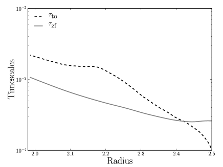
Figure 15: Radial profiles of the two timescales defined in Eq. (40): turnover timescale of convection (dashed black line) and timescale associated with shear (solid grey line). These profiles have been derived from an azimuthal average of the values in the equatorial plane for a model with $N_{\rho}=5$ and $\text{Ra}=4\times 10^{7}$ (same model as in Fig. 14).

As demonstrated above for stronger stratifications (see Fig. 5), $H_{\rho}$ decreases outward while $u_{\text{conv}}$ increases. This leads to a shorter turnover timescale close to the surface. Therefore, surface plumes that could potentially help to generate vorticity via the compressional source have a too short lifetime to significantly foster Reynolds stresses. In the deeper part, the extra efficiency gained by compressible effects is limited, explaining why zonal jets of compressible and Boussinesq simulations are found to be similar.

5 Conclusion

We have investigated the effects of compressibility in 3-D rapidly rotating convection. Following Gilman and Glatzmaier (1981), Jones and Kuzanyan (2009) and Kaspi et al. (2009), all the simulations have been computed under the anelastic approximation. As we focus on the effects of the density stratification, we have deliberately chosen a moderate Ekman number of $10^{-4}$, which allowed us to reach more supercritical Rayleigh numbers. From the simulations computed in this parametric study, we highlight the following results:

• Concerning the onset of convection, an increase of the density stratification is accompanied with a strong confinement of the convective columns close to the outer boundary as well as an increase of the critical azimuthal wavenumber, in agreement with the results of the linear stability of Jones et al. (2009). This gradual outward shift of the onset of convection is explained by the radial increase of buoyancy.

• When increasing supercriticality, the solutions which simply drift close to onset, start to vacillate, then become intermittent and finally chaotic (Grote and Busse, 2001). While these different regimes are clearly separated in the Boussinesq cases, the transitions occupy a shorter fraction of the parameter space with increase of density stratification.

• For stronger background density stratifications, the convective flow amplitude increases outward, while the lengthscale decreases. Concerning zonal winds, Boussinesq and anelastic simulations show very similar properties, provided the convection is strongly driven: both the extent and the number of jets become fairly independent of the density background. This suggests that zonal flows follow a universal behaviour, independent of the density stratification, and may also explain why Boussinesq models were already very successful in reproducing the morphology of the jets observed in gas giants (e.g. Heimpel et al., 2005).

• In the strongly nonlinear regime, the solutions seem to follow the same asymptotic scaling laws, independently of the density stratification. Convective Rossby number and Nusselt number follow previously studied laws (Christensen, 2002). The scaling of the total Rossby number differs slightly from that suggested by Showman et al. (2011), which may be attributed to the different model used by these authors. The obtained scaling laws allow us to extrapolate our simulations to Jupiter. Taking an internal heat flux of $5.44\text{~{}W.}\text{m}^{-2}$ (Hanel et al., 1981), $\Omega=1.75\times 10^{-4}\text{~{}s}^{-1}$, $c_{p}=1.3\times 10^{4}\text{~{}J.kg}^{-1}\text{.K}^{-1}$ and $d=1.2\times 10^{4}\text{~{}kms}$, the evolution models of Guillot et al. (2004) suggest that the flux-based Rayleigh number decreases from $\text{Ra}_{q}^{*}\sim 5\times 10^{-7}$ at the surface to $\text{Ra}_{q}^{*}\sim 3\times 10^{-12}$ at the bottom of the molecular envelope (i.e. $\eta=0.85$). This leads to a mass-weighted flux based Rayleigh number of $\langle\text{Ra}_{q}^{*}\rangle_{\rho}\sim 1.2\times 10^{-11}$. Our scaling law (Eq. 30) then predicts a Rossby number of $6\times 10^{-4}$, which corresponds to an average zonal velocity around $1\text{~{}m.}\text{s}^{-1}$. In agreement with the previous extrapolations of Showman et al. (2011), this value is much weaker (about one order of magnitude) than the surface zonal winds of gas giants. This rescaling is however tentative as the scaling laws may still depend on other parameters that have been kept constant in this study, for example Ekman number, Prandtl number or aspect ratio, and further simulations would be required to clarify this.

• The zonal jets are maintained by Reynolds stresses, which rely on the correlation between zonal ($u_{\phi}$) and cylindrically radial ($u_{s}$) flow components. The gradual loss of this correlation with increasing supercriticality hampers all our simulations, independently of the background density stratification. However in the strongly stratified simulations, the correlation is first lost in the outer part of the flow, where compressibility effects are most significant. Because of the short lengthscales and the large flow amplitudes found there, the fluid parcels loose their identity before interacting efficiently with the zonal flows. This may explain why the additional compressional source of vorticity has not the important effect expected by Evonuk (2008) and Glatzmaier et al. (2009) in our simulations. However, the influence of the different vorticity contributions are hard to disentangle in 3-D compressible convection, stressing the need of future theoretical work to address this question.

All the results obtained in this study have been derived in a non-conducting layer, where magnetic effects have been neglected. Nevertheless, as suggested by Liu et al. (2008), the Ohmic dissipation associated with the outer semi-conducting region could strongly limit the extent of the surface jets. Addressing this problem would require 3-D dynamo simulations of compressible convection with variable conductivity (Stanley and Glatzmaier, 2010; Heimpel and Gómez Pérez, 2011).

Table 2: List of numerical simulations presented in this work. For all the simulations, $\text{E}=10^{-4}$ and $\text{Pr}=1$.

${Ra}/{Ra}_{\text{crit}}$	$\langle\text{Ro}\rangle_{\rho}$	$\langle\text{Ro}_{\text{pol}}\rangle_{\rho}$	$E_{\text{tor}}^{m=0}/E_{\text{kin}}$	Nu
$N_{\rho}=10^{-2}$, symbol=red circle
$1.0006$	$4.49\times 10^{-5}$	$2.49\times 10^{-5}$	$0.002$	$1.0002$
$1.0063$	$1.03\times 10^{-4}$	$5.71\times 10^{-5}$	$0.011$	$1.0009$
$1.035$	$2.35\times 10^{-4}$	$1.26\times 10^{-4}$	$0.058$	$1.0045$
$1.15$	$5.04\times 10^{-4}$	$2.45\times 10^{-4}$	$0.231$	$1.016$
$1.72$	$1.25\times 10^{-3}$	$4.41\times 10^{-4}$	$0.586$	$1.045$
$2.01$	$1.52\times 10^{-3}$	$4.96\times 10^{-4}$	$0.640$	$1.053$
$2.30$	$1.98\times 10^{-3}$	$5.86\times 10^{-4}$	$0.700$	$1.067$
$2.87$	$2.85\times 10^{-3}$	$7.19\times 10^{-4}$	$0.773$	$1.087$
$3.45$	$3.37\times 10^{-3}$	$8.23\times 10^{-4}$	$0.788$	$1.104$
$4.60$	$5.05\times 10^{-3}$	$1.24\times 10^{-3}$	$0.816$	$1.1800$
$5.75$	$7.18\times 10^{-3}$	$1.58\times 10^{-3}$	$0.843$	$1.23$
$7.47$	$1.16\times 10^{-2}$	$2.03\times 10^{-3}$	$0.902$	$1.31$
$8.62$	$1.44\times 10^{-2}$	$2.35\times 10^{-3}$	$0.916$	$1.37$
$10.35$	$1.95\times 10^{-2}$	$2.97\times 10^{-3}$	$0.929$	$1.51$
$11.50$	$2.24\times 10^{-2}$	$3.38\times 10^{-3}$	$0.933$	$1.61$
$14.37$	$3.09\times 10^{-2}$	$4.51\times 10^{-3}$	$0.942$	$1.89$
$17.25$	$3.90\times 10^{-2}$	$5.62\times 10^{-3}$	$0.945$	$2.20$
$20.12$	$4.51\times 10^{-2}$	$6.67\times 10^{-3}$	$0.943$	$2.52$
$23.00$	$5.20\times 10^{-2}$	$7.96\times 10^{-3}$	$0.939$	$2.89$
$28.75$	$6.34\times 10^{-2}$	$1.04\times 10^{-2}$	$0.932$	$3.65$
$34.50$	$7.30\times 10^{-2}$	$1.27\times 10^{-2}$	$0.924$	$4.44$
$40.25$	$8.30\times 10^{-2}$	$1.52\times 10^{-2}$	$0.915$	$5.29$
$46.00$	$9.10\times 10^{-2}$	$1.77\times 10^{-2}$	$0.903$	$6.04$
$51.75$	$9.98\times 10^{-2}$	$2.00\times 10^{-2}$	$0.893$	$6.81$
$57.50$	$1.09\times 10^{-1}$	$2.24\times 10^{-2}$	$0.883$	$7.60$
$69.00$	$1.21\times 10^{-1}$	$2.73\times 10^{-2}$	$0.874$	$9.22$
$86.25$	$1.42\times 10^{-1}$	$3.40\times 10^{-2}$	$0.863$	$11.53$
$115.0$	$1.79\times 10^{-1}$	$4.78\times 10^{-2}$	$0.845$	$16.21$
$143.7$	$2.03\times 10^{-1}$	$5.74\times 10^{-2}$	$0.830$	$19.50$
$N_{\rho}=2$, symbol=blue triangle
$1.0001$	$3.65\times 10^{-5}$	$2.63\times 10^{-5}$	$0.001$	$1.0001$
$1.0035$	$9.13\times 10^{-5}$	$6.77\times 10^{-5}$	$0.007$	$1.0005$
$1.0079$	$1.28\times 10^{-4}$	$9.57\times 10^{-5}$	$0.014$	$1.0010$
$1.051$	$2.80\times 10^{-4}$	$1.99\times 10^{-4}$	$0.093$	$1.0045$
$1.13$	$5.96\times 10^{-4}$	$3.75\times 10^{-4}$	$0.339$	$1.013$
$1.31$	$1.56\times 10^{-3}$	$7.12\times 10^{-4}$	$0.636$	$1.040$
$1.57$	$3.94\times 10^{-3}$	$1.32\times 10^{-3}$	$0.782$	$1.11$
$1.75$	$6.15\times 10^{-3}$	$1.74\times 10^{-3}$	$0.838$	$1.17$
$1.92$	$7.95\times 10^{-3}$	$1.94\times 10^{-3}$	$0.877$	$1.20$
$2.19$	$1.07\times 10^{-2}$	$2.29\times 10^{-3}$	$0.903$	$1.26$
$2.45$	$1.35\times 10^{-2}$	$2.61\times 10^{-3}$	$0.920$	$1.31$
$2.62$	$1.50\times 10^{-2}$	$2.81\times 10^{-3}$	$0.925$	$1.35$
$3.06$	$2.04\times 10^{-2}$	$3.49\times 10^{-3}$	$0.936$	$1.49$
$3.50$	$2.53\times 10^{-2}$	$4.11\times 10^{-3}$	$0.940$	$1.64$
$4.38$	$3.43\times 10^{-2}$	$5.44\times 10^{-3}$	$0.941$	$1.97$
$5.25$	$4.24\times 10^{-2}$	$6.81\times 10^{-3}$	$0.938$	$2.38$
$6.13$	$5.10\times 10^{-2}$	$8.57\times 10^{-3}$	$0.931$	$2.94$
$7.01$	$5.27\times 10^{-2}$	$1.05\times 10^{-2}$	$0.905$	$3.52$
$8.76$	$6.80\times 10^{-2}$	$1.40\times 10^{-2}$	$0.900$	$4.64$
$13.14$	$1.03\times 10^{-1}$	$2.16\times 10^{-2}$	$0.904$	$6.98$
$17.52$	$1.35\times 10^{-1}$	$2.88\times 10^{-2}$	$0.902$	$9.38$
$26.29$	$1.80\times 10^{-1}$	$4.10\times 10^{-2}$	$0.896$	$13.33$
$N_{\rho}=4$, symbol=dark blue pentagon
$1.0005$	$2.52\times 10^{-5}$	$2.02\times 10^{-5}$	$0.000$	$1.0002$
$1.0016$	$3.63\times 10^{-5}$	$3.02\times 10^{-5}$	$0.000$	$1.0005$
$1.0097$	$8.11\times 10^{-5}$	$6.89\times 10^{-5}$	$0.002$	$1.0025$
$1.025$	$1.34\times 10^{-4}$	$1.11\times 10^{-4}$	$0.006$	$1.0063$
$1.079$	$2.21\times 10^{-4}$	$1.82\times 10^{-4}$	$0.039$	$1.017$
$1.34$	$4.11\times 10^{-4}$	$2.96\times 10^{-4}$	$0.280$	$1.037$
$1.61$	$6.76\times 10^{-4}$	$4.00\times 10^{-4}$	$0.462$	$1.054$
$1.88$	$1.09\times 10^{-3}$	$5.50\times 10^{-4}$	$0.607$	$1.078$
$2.15$	$1.69\times 10^{-3}$	$7.32\times 10^{-4}$	$0.706$	$1.109$
$2.69$	$3.41\times 10^{-3}$	$1.18\times 10^{-3}$	$0.809$	$1.21$
$3.23$	$5.70\times 10^{-3}$	$1.68\times 10^{-3}$	$0.854$	$1.35$
$3.77$	$8.52\times 10^{-3}$	$2.20\times 10^{-3}$	$0.877$	$1.50$
$4.31$	$1.20\times 10^{-2}$	$3.05\times 10^{-3}$	$0.869$	$1.92$
$5.39$	$1.96\times 10^{-2}$	$4.43\times 10^{-3}$	$0.893$	$2.52$
$7.01$	$3.03\times 10^{-2}$	$6.25\times 10^{-3}$	$0.907$	$3.29$
$8.63$	$3.89\times 10^{-2}$	$7.61\times 10^{-3}$	$0.916$	$3.70$
$10.79$	$5.04\times 10^{-2}$	$9.62\times 10^{-3}$	$0.919$	$4.48$
$14.03$	$6.57\times 10^{-2}$	$1.25\times 10^{-2}$	$0.920$	$5.49$
$17.27$	$7.80\times 10^{-2}$	$1.51\times 10^{-2}$	$0.917$	$6.56$
$21.59$	$8.86\times 10^{-2}$	$1.81\times 10^{-2}$	$0.909$	$7.87$
$26.99$	$1.05\times 10^{-1}$	$2.23\times 10^{-2}$	$0.904$	$8.65$
$32.39$	$1.16\times 10^{-1}$	$2.61\times 10^{-2}$	$0.896$	$9.73$

${Ra}/{Ra}_{\text{crit}}$	$\langle\text{Ro}\rangle_{\rho}$	$\langle\text{Ro}_{\text{pol}}\rangle_{\rho}$	$E_{\text{tor}}^{m=0}/E_{\text{kin}}$	Nu
$N_{\rho}=1$, symbol=green triangle
$1.0010$	$5.36\times 10^{-5}$	$3.66\times 10^{-5}$	$0.002$	$1.0001$
$1.0068$	$1.31\times 10^{-4}$	$8.82\times 10^{-5}$	$0.014$	$1.0008$
$1.0145$	$1.95\times 10^{-4}$	$1.30\times 10^{-4}$	$0.033$	$1.0018$
$1.024$	$2.54\times 10^{-4}$	$1.67\times 10^{-4}$	$0.055$	$1.0029$
$1.062$	$4.23\times 10^{-4}$	$2.58\times 10^{-4}$	$0.156$	$1.007$
$1.15$	$6.99\times 10^{-4}$	$3.79\times 10^{-4}$	$0.357$	$1.009$
$1.35$	$1.15\times 10^{-3}$	$5.29\times 10^{-4}$	$0.537$	$1.028$
$1.44$	$1.48\times 10^{-3}$	$6.17\times 10^{-4}$	$0.619$	$1.036$
$1.54$	$1.78\times 10^{-3}$	$6.88\times 10^{-4}$	$0.674$	$1.044$
$1.73$	$2.40\times 10^{-3}$	$8.13\times 10^{-4}$	$0.748$	$1.058$
$1.93$	$3.11\times 10^{-3}$	$9.47\times 10^{-4}$	$0.795$	$1.07$
$2.51$	$6.21\times 10^{-3}$	$1.48\times 10^{-3}$	$0.858$	$1.14$
$2.89$	$9.23\times 10^{-3}$	$1.97\times 10^{-3}$	$0.885$	$1.23$
$3.28$	$1.15\times 10^{-2}$	$2.20\times 10^{-3}$	$0.905$	$1.26$
$3.86$	$1.59\times 10^{-2}$	$2.71\times 10^{-3}$	$0.925$	$1.37$
$4.83$	$2.00\times 10^{-2}$	$3.57\times 10^{-3}$	$0.922$	$1.49$
$5.79$	$2.61\times 10^{-2}$	$4.43\times 10^{-3}$	$0.931$	$1.69$
$7.72$	$3.92\times 10^{-2}$	$6.28\times 10^{-3}$	$0.937$	$2.17$
$9.66$	$4.91\times 10^{-2}$	$8.39\times 10^{-3}$	$0.927$	$2.79$
$11.59$	$5.83\times 10^{-2}$	$1.08\times 10^{-2}$	$0.916$	$3.42$
$13.52$	$6.74\times 10^{-2}$	$1.31\times 10^{-2}$	$0.909$	$4.14$
$15.45$	$7.63\times 10^{-2}$	$1.53\times 10^{-2}$	$0.904$	$4.86$
$19.32$	$9.45\times 10^{-2}$	$2.02\times 10^{-2}$	$0.896$	$6.41$
$23.18$	$1.12\times 10^{-1}$	$2.48\times 10^{-2}$	$0.893$	$7.84$
$28.98$	$1.38\times 10^{-1}$	$3.04\times 10^{-2}$	$0.875$	$9.69$
$38.64$	$1.71\times 10^{-1}$	$3.95\times 10^{-2}$	$0.873$	$12.86$
$48.30$	$1.98\times 10^{-1}$	$4.87\times 10^{-2}$	$0.871$	$15.97$
$N_{\rho}=3$, symbol=magenta diamond
$1.0020$	$4.24\times 10^{-5}$	$3.32\times 10^{-5}$	$0.001$	$1.0003$
$1.0039$	$6.35\times 10^{-5}$	$5.15\times 10^{-5}$	$0.002$	$1.0007$
$1.0072$	$9.32\times 10^{-5}$	$7.21\times 10^{-5}$	$0.004$	$1.0013$
$1.013$	$1.27\times 10^{-4}$	$1.01\times 10^{-4}$	$0.008$	$1.0025$
$1.046$	$2.29\times 10^{-4}$	$1.75\times 10^{-4}$	$0.037$	$1.0076$
$1.11$	$3.14\times 10^{-4}$	$2.30\times 10^{-4}$	$0.111$	$1.0134$
$1.24$	$5.17\times 10^{-4}$	$3.35\times 10^{-4}$	$0.307$	$1.024$
$1.63$	$1.75\times 10^{-3}$	$7.85\times 10^{-4}$	$0.675$	$1.074$
$1.83$	$2.91\times 10^{-3}$	$1.09\times 10^{-3}$	$0.770$	$1.11$
$1.96$	$3.80\times 10^{-3}$	$1.27\times 10^{-3}$	$0.812$	$1.13$
$2.28$	$6.30\times 10^{-3}$	$1.75\times 10^{-3}$	$0.866$	$1.20$
$2.61$	$9.09\times 10^{-3}$	$2.15\times 10^{-3}$	$0.899$	$1.27$
$3.27$	$1.47\times 10^{-2}$	$2.99\times 10^{-3}$	$0.920$	$1.45$
$3.92$	$2.07\times 10^{-2}$	$3.95\times 10^{-3}$	$0.924$	$1.76$
$4.57$	$2.62\times 10^{-2}$	$4.90\times 10^{-3}$	$0.922$	$2.09$
$5.23$	$3.21\times 10^{-2}$	$5.84\times 10^{-3}$	$0.924$	$2.42$
$5.88$	$3.77\times 10^{-2}$	$6.91\times 10^{-3}$	$0.922$	$2.81$
$7.19$	$4.91\times 10^{-2}$	$8.94\times 10^{-3}$	$0.922$	$3.51$
$9.81$	$6.66\times 10^{-2}$	$1.28\times 10^{-2}$	$0.916$	$4.80$
$13.08$	$8.48\times 10^{-2}$	$1.74\times 10^{-2}$	$0.908$	$6.30$
$16.35$	$1.03\times 10^{-1}$	$2.17\times 10^{-2}$	$0.905$	$7.84$
$20.92$	$1.25\times 10^{-1}$	$2.70\times 10^{-2}$	$0.902$	$9.47$
$26.16$	$1.47\times 10^{-1}$	$3.28\times 10^{-2}$	$0.900$	$11.76$
$32.70$	$1.70\times 10^{-1}$	$4.09\times 10^{-2}$	$0.886$	$14.14$
$N_{\rho}=5$, symbol=orange square
$1.0017$	$2.49\times 10^{-5}$	$2.24\times 10^{-5}$	$0.000$	$1.0005$
$1.0038$	$3.56\times 10^{-5}$	$3.21\times 10^{-5}$	$0.001$	$1.0011$
$1.025$	$9.09\times 10^{-5}$	$8.06\times 10^{-5}$	$0.003$	$1.0066$
$1.067$	$1.50\times 10^{-4}$	$1.33\times 10^{-4}$	$0.013$	$1.017$
$1.28$	$2.71\times 10^{-4}$	$2.19\times 10^{-4}$	$0.124$	$1.041$
$1.70$	$4.61\times 10^{-4}$	$3.10\times 10^{-4}$	$0.351$	$1.061$
$2.13$	$8.20\times 10^{-4}$	$4.50\times 10^{-4}$	$0.548$	$1.104$
$2.56$	$1.32\times 10^{-3}$	$6.19\times 10^{-4}$	$0.661$	$1.163$
$2.99$	$1.96\times 10^{-3}$	$8.10\times 10^{-4}$	$0.726$	$1.24$
$3.41$	$2.82\times 10^{-3}$	$1.08\times 10^{-3}$	$0.751$	$1.37$
$3.84$	$3.92\times 10^{-3}$	$1.44\times 10^{-3}$	$0.759$	$1.57$
$4.27$	$5.04\times 10^{-3}$	$1.77\times 10^{-3}$	$0.766$	$1.77$
$5.55$	$9.65\times 10^{-3}$	$2.92\times 10^{-3}$	$0.821$	$2.37$
$6.40$	$1.30\times 10^{-2}$	$3.56\times 10^{-3}$	$0.853$	$2.67$
$7.68$	$1.82\times 10^{-2}$	$4.45\times 10^{-3}$	$0.881$	$3.06$
$11.11$	$3.09\times 10^{-2}$	$6.65\times 10^{-3}$	$0.904$	$4.01$
$13.67$	$3.99\times 10^{-2}$	$8.17\times 10^{-3}$	$0.911$	$4.68$
$17.09$	$5.03\times 10^{-2}$	$1.01\times 10^{-2}$	$0.914$	$5.45$
$21.36$	$6.26\times 10^{-2}$	$1.26\times 10^{-2}$	$0.914$	$6.52$
$25.63$	$6.94\times 10^{-2}$	$1.40\times 10^{-2}$	$0.915$	$6.87$
$32.04$	$7.85\times 10^{-2}$	$1.63\times 10^{-2}$	$0.911$	$8.04$

References

- Anufriev et al. (2005) Anufriev, A.P., Jones, C.A., Soward, A.M., 2005. The Boussinesq and anelastic liquid approximations for convection in the Earth’s core. Physics of the Earth and Planetary Interiors 152, 163–190.
- Atkinson et al. (1997) Atkinson, D.H., Ingersoll, A.P., Seiff, A., 1997. Deep winds on Jupiter as measured by the Galileo probe. Nature 388, 649–650.
- Aurnou et al. (2007) Aurnou, J., Heimpel, M., Wicht, J., 2007. The effects of vigorous mixing in a convective model of zonal flow on the ice giants. Icarus 190, 110–126.
- Ballot et al. (2007) Ballot, J., Brun, A.S., Turck-Chièze, S., 2007. Simulations of turbulent convection in rotating young solarlike stars: differential rotation and meridional circulation. ApJ 669, 1190–1208.
- Böhm-Vitense (1958) Böhm-Vitense, E., 1958. Über die Wasserstoffkonvektionszone in Sternen verschiedener Effektivtemperaturen und Leuchtkräfte. Zeitschrift für Astrophysik 46, 108–143.
- Braginsky and Roberts (1995) Braginsky, S.I., Roberts, P.H., 1995. Equations governing convection in earth’s core and the geodynamo. Geophysical and Astrophysical Fluid Dynamics 79, 1–97.
- Busse (1983) Busse, F.H., 1983. A model of mean zonal flows in the major planets. Geophysical and Astrophysical Fluid Dynamics 23, 153–174.
- Busse (1994) Busse, F.H., 1994. Convection driven zonal flows and vortices in the major planets. Chaos 4, 123–134.
- Busse (2002) Busse, F.H., 2002. Convective flows in rapidly rotating spheres and their dynamo action. Physics of Fluids 14, 1301–1314.
- Cho and Polvani (1996) Cho, J., Polvani, L.M., 1996. The morphogenesis of bands and zonal winds in the atmospheres on the giant outer planets. Science 273, 335–337.
- Christensen and Wicht (2007) Christensen, U., Wicht, J., 2007. Numerical dynamo simulations. pp. 97–114.
- Christensen (2001) Christensen, U.R., 2001. Zonal flow driven by deep convection in the major planets. Geophys. Res. Lett. 28, 2553–2556.
- Christensen (2002) Christensen, U.R., 2002. Zonal flow driven by strongly supercritical convection in rotating spherical shells. Journal of Fluid Mechanics 470, 115–133.
- Christensen and Aubert (2006) Christensen, U.R., Aubert, J., 2006. Scaling properties of convection-driven dynamos in rotating spherical shells and application to planetary magnetic fields. Geophysical Journal International 166, 97–114.
- Evonuk (2008) Evonuk, M., 2008. The role of density stratification in generating zonal flow structures in a rotating fluid. ApJ 673, 1154–1159.
- Fernando et al. (1991) Fernando, H.J.S., Chen, R.R., Boyer, D.L., 1991. Effects of rotation on convective turbulence. Journal of Fluid Mechanics 228, 513–547.
- Gilman and Glatzmaier (1981) Gilman, P.A., Glatzmaier, G.A., 1981. Compressible convection in a rotating spherical shell - I - Anelastic equations. ApJS 45, 335–349.
- Glatzmaier et al. (2009) Glatzmaier, G., Evonuk, M., Rogers, T., 2009. Differential rotation in giant planets maintained by density-stratified turbulent convection. Geophysical and Astrophysical Fluid Dynamics 103, 31–51.
- Glatzmaier (2008) Glatzmaier, G.A., 2008. A note on “Constraints on deep-seated zonal winds inside Jupiter and Saturn”. Icarus 196, 665–666.
- Glatzmaier and Gilman (1981) Glatzmaier, G.A., Gilman, P.A., 1981. Compressible convection in a rotating spherical shell - II - A linear anelastic model. ApJS 45, 351–380.
- Gough et al. (1976) Gough, D.O., Moore, D.R., Spiegel, E.A., Weiss, N.O., 1976. Convective instability in a compressible atmosphere. II. ApJ 206, 536–542.
- Grote and Busse (2001) Grote, E., Busse, F.H., 2001. Dynamics of convection and dynamos in rotating spherical fluid shells. Fluid Dynamics Research 28, 349–368.
- Guillot (1999) Guillot, T., 1999. Interior of Giant Planets Inside and Outside the Solar System. Science 286, 72–77.
- Guillot et al. (2004) Guillot, T., Stevenson, D.J., Hubbard, W.B., Saumon, D., 2004. The interior of Jupiter. pp. 35–57.
- Hanel et al. (1981) Hanel, R., Conrath, B., Herath, L., Kunde, V., Pirraglia, J., 1981. Albedo, internal heat, and energy balance of Jupiter - Preliminary results of the Voyager infrared investigation. J. Geophys. Res. 86, 8705–8712.
- Heimpel et al. (2005) Heimpel, M., Aurnou, J., Wicht, J., 2005. Simulation of equatorial and high-latitude jets on Jupiter in a deep convection model. Nature 438, 193–196.
- Heimpel and Aurnou (2012) Heimpel, M., Aurnou, J.M., 2012. Convective Bursts and the Coupling of Saturn’s Equatorial Storms and Interior Rotation. ApJ 746, 51.
- Heimpel and Gómez Pérez (2011) Heimpel, M., Gómez Pérez, N., 2011. On the relationship between zonal jets and dynamo action in giant planets. Geophys. Res. Lett. 38, L14201.
- Jones et al. (2011) Jones, C.A., Boronski, P., Brun, A.S., Glatzmaier, G.A., Gastine, T., Miesch, M.S., Wicht, J., 2011. Anelastic convection-driven dynamo benchmarks. Icarus 216, 120–135.
- Jones and Kuzanyan (2009) Jones, C.A., Kuzanyan, K.M., 2009. Compressible convection in the deep atmospheres of giant planets. Icarus 204, 227–238.
- Jones et al. (2009) Jones, C.A., Kuzanyan, K.M., Mitchell, R.H., 2009. Linear theory of compressible convection in rapidly rotating spherical shells, using the anelastic approximation. Journal of Fluid Mechanics 634, 291–319.
- Kaspi et al. (2009) Kaspi, Y., Flierl, G.R., Showman, A.P., 2009. The deep wind structure of the giant planets: Results from an anelastic general circulation model. Icarus 202, 525–542.
- Lantz and Fan (1999) Lantz, S.R., Fan, Y., 1999. Anelastic magnetohydrodynamic equations for modeling solar and stellar convection zones. ApJS 121, 247–264.
- Lian and Showman (2010) Lian, Y., Showman, A.P., 2010. Generation of equatorial jets by large-scale latent heating on the giant planets. Icarus 207, 373–393.
- Liu et al. (2008) Liu, J., Goldreich, P.M., Stevenson, D.J., 2008. Constraints on deep-seated zonal winds inside Jupiter and Saturn. Icarus 196, 653–664.
- Nellis (2000) Nellis, W.J., 2000. Metallization of fluid hydrogen at 140 GPa (1.4 Mbar): implications for Jupiter. Planet. Space Sci. 48, 671–677.
- Nellis et al. (1996) Nellis, W.J., Weir, S.T., Mitchell, A.C., 1996. Metallization and electrical conductivity of Hydrogen in Jupiter. Science 273, 936–938.
- Nettelmann et al. (2008) Nettelmann, N., Holst, B., Kietzmann, A., French, M., Redmer, R., Blaschke, D., 2008. Ab Initio equation of state data for Hydrogen, Helium, and water and the internal structure of Jupiter. ApJ 683, 1217–1228.
- Plaut et al. (2008) Plaut, E., Lebranchu, Y., Simitev, R., Busse, F.H., 2008. Reynolds stresses and mean fields generated by pure waves: applications to shear flows and convection in a rotating shell. Journal of Fluid Mechanics 602, 303–326.
- Porco et al. (2003) Porco, C.C., West, R.A., McEwen, A., Del Genio, A.D., Ingersoll, A.P., Thomas, P., Squyres, S., Dones, L., Murray, C.D., Johnson, T.V., Burns, J.A., Brahic, A., Neukum, G., Veverka, J., Barbara, J.M., Denk, T., Evans, M., Ferrier, J.J., Geissler, P., Helfenstein, P., Roatsch, T., Throop, H., Tiscareno, M., Vasavada, A.R., 2003. Cassini Imaging of Jupiter’s Atmosphere, Satellites, and Rings. Science 299, 1541–1547.
- Salyk et al. (2006) Salyk, C., Ingersoll, A.P., Lorre, J., Vasavada, A., Del Genio, A.D., 2006. Interaction between eddies and mean flow in Jupiter’s atmosphere: Analysis of Cassini imaging data. Icarus 185, 430–442.
- Schaeffer and Cardin (2005) Schaeffer, N., Cardin, P., 2005. Quasigeostrophic model of the instabilities of the Stewartson layer in flat and depth-varying containers. Physics of Fluids 17, 104111.
- Scott and Polvani (2008) Scott, R.K., Polvani, L.M., 2008. Equatorial superrotation in shallow atmospheres. Geophys. Res. Lett. 35, 24202.
- Showman et al. (2011) Showman, A.P., Kaspi, Y., Flierl, G.R., 2011. Scaling laws for convection and jet speeds in the giant planets. Icarus 211, 1258–1273.
- Simitev and Busse (2003) Simitev, R., Busse, F.H., 2003. Patterns of convection in rotating spherical shells. New Journal of Physics 5, 97.
- Stanley and Glatzmaier (2010) Stanley, S., Glatzmaier, G.A., 2010. Dynamo models for planets other than Earth. Space Sci. Rev. 152, 617–649.
- Tortorella (2005) Tortorella, D.A., 2005. Numerical studies of thermal and compressible convection in rotating spherical shells: an application to the giant planets. Ph.D. thesis. International Max Planck Research School, Universities of Braunschweig and Göttingen, Germany.
- Unno et al. (1960) Unno, W., Kato, S., Makita, M., 1960. Convective instability in polytropic atmospheres, I. PASJ 12, 192–202.
- Vasavada and Showman (2005) Vasavada, A.R., Showman, A.P., 2005. Jovian atmospheric dynamics: an update after Galileo and Cassini. Reports on Progress in Physics 68, 1935–1996.
- Vitense (1953) Vitense, E., 1953. Die Wasserstoffkonvektionszone der Sonne. Zeitschrift für Astrophysik 32, 135–164.
- Wicht (2002) Wicht, J., 2002. Inner-core conductivity in numerical dynamo simulations. Physics of the Earth and Planetary Interiors 132, 281–302.
- Williams (1978) Williams, G.P., 1978. Planetary circulations. I - Barotropic representation of Jovian and terrestrial turbulence. Journal of Atmospheric Sciences 35, 1399–1426.
- Zhang (1992) Zhang, K., 1992. Spiralling columnar convection in rapidly rotating spherical fluid shells. Journal of Fluid Mechanics 236, 535–556.