Numerical point of view on Calculus for functions assuming finite, infinite, and infinitesimal values over finite, infinite, and infinitesimal domains

Abstract

The goal of this paper consists of developing a new (more physical and numerical in comparison with standard and non-standard analysis approaches) point of view on Calculus with functions assuming infinite and infinitesimal values. It uses recently introduced infinite and infinitesimal numbers being in accordance with the principle ‘The part is less than the whole’ observed in the physical world around us. These numbers have a strong practical advantage with respect to traditional approaches: they are representable at a new kind of a computer – the Infinity Computer – able to work numerically with all of them. An introduction to the theory of physical and mathematical continuity and differentiation (including subdifferentials) for functions assuming finite, infinite, and infinitesimal values over finite, infinite, and infinitesimal domains is developed in the paper. This theory allows one to work with derivatives that can assume not only finite but infinite and infinitesimal values, as well. It is emphasized that the newly introduced notion of the physical continuity allows one to see the same mathematical object as a continuous or a discrete one, in dependence on the wish of the researcher, i.e., as it happens in the physical world where the same object can be viewed as a continuous or a discrete in dependence on the instrument of the observation used by the researcher. Connections between pure mathematical concepts and their computational realizations are continuously emphasized through the text. Numerous examples are given.

Key Words: Infinite and infinitesimal numbers and numerals; infinite and infinitesimal functions and derivatives; physical and mathematical notions of continuity.

1 Introduction

Numerous trials have been done during the centuries in order to evolve existing numeral systems in such a way that infinite and infinitesimal numbers could be included in them (see [1, 2, 5, 9, 10, 13, 23]). Particularly, in the early history of the calculus, arguments involving infinitesimals played a pivotal role in the derivation developed by Leibniz and Newton (see [9, 10]). The notion of an infinitesimal, however, lacked a precise mathematical definition and in order to provide a more rigorous foundation for the calculus infinitesimals were gradually replaced by the d’Alembert-Cauchy concept of a limit (see [3, 7]).

The creation of a mathematical theory of infinitesimals on which to base the calculus remained an open problem until the end of the 1950s when Robinson (see [13]) introduced his famous non-standard Analysis approach. He has shown that non-archimedean ordered field extensions of the reals contained numbers that could serve the role of infinitesimals and their reciprocals could serve as infinitely large numbers. Robinson then has derived the theory of limits, and more generally of Calculus, and has found a number of important applications of his ideas in many other fields of Mathematics (see [13]).

In his approach, Robinson used mathematical tools and terminology (cardinal numbers, countable sets, continuum, one-to-one correspondence, etc.) taking their origins from the famous ideas of Cantor (see [2]) who has shown that there existed infinite sets having different number of elements. It is well known nowadays that while dealing with infinite sets, Cantor’s approach leads to some counterintuitive situations that often are called by non-mathematicians ‘paradoxes’. For example, the set of even numbers, $\mathbb{E}$, can be put in a one-to-one correspondence with the set of all natural numbers, $\mathbb{N}$, in spite of the fact that $\mathbb{E}$ is a part of $\mathbb{N}$:

$$\begin{array}[]{lccccccc}\mbox{even numbers:}&\hskip 14.22636pt2,&4,&6,&8,&10,&12,&\ldots\\ &\hskip 14.22636pt\updownarrow&\updownarrow&\updownarrow&\updownarrow&\updownarrow&\updownarrow&\\ \mbox{natural numbers:}&\hskip 14.22636pt1,&2,&3,&4&5,&6,&\ldots\\ \end{array}$$ (1)

The philosophical principle of Ancient Greeks ‘The part is less than the whole’ observed in the world around us does not hold true for infinite numbers introduced by Cantor, e.g., it follows $x+1=x$, if $x$ is an infinite cardinal, although for any finite $x$ we have $x+1>x$. As a consequence, the same effects necessary have reflections in the non-standard Analysis of Robinson (this is not the case of the interesting non-standard approach introduced recently in [1]).

Due to the enormous importance of the concepts of infinite and infinitesimal in science, people try to introduce them in their work with computers, too (see, e.g. the IEEE Standard for Binary Floating-Point Arithmetic). However, non-standard Analysis remains a very theoretical field because various arithmetics (see [1, 2, 5, 13]) developed for infinite and infinitesimal numbers are quite different with respect to the finite arithmetic we are used to deal with. Very often they leave undetermined many operations where infinite numbers take part (for example, $\infty-\infty$, $\frac{\infty}{\infty}$, sum of infinitely many items, etc.) or use representation of infinite numbers based on infinite sequences of finite numbers. These crucial difficulties did not allow people to construct computers that would be able to work with infinite and infinitesimal numbers in the same manner as we are used to do with finite numbers and to study infinite and infinitesimal objects numerically.

Recently a new applied point of view on infinite and infinitesimal numbers has been introduced in [14, 18, 21]. The new approach does not use Cantor’s ideas and describes infinite and infinitesimal numbers that are in accordance with the principle ‘The part is less than the whole’. It gives a possibility to work with finite, infinite, and infinitesimal quantities numerically by using a new kind of a computer – the Infinity Computer – introduced in [15, 16, 17]. It is worthwhile noticing that the new approach does not contradict Cantor. In contrast, it can be viewed as an evolution of his deep ideas regarding the existence of different infinite numbers in a more applied way. For instance, Cantor has shown that there exist infinite sets having different cardinalities $\aleph_{0}$ and $\aleph_{1}$. In its turn, the new approach specifies this result showing that in certain cases within each of these classes it is possible to distinguish sets with the number of elements being different infinite numbers.

The goal of this paper consists of developing a new (more physical and numerical in comparison with standard and non-standard Analysis approaches) point of view on Calculus. On the one hand, it uses the approach introduced in [14, 18, 21] and, on the other hand, it incorporates in Calculus the following two main ideas.

i) Note that foundations of Analysis have been developed more than 200 years ago with the goal to develop mathematical tools allowing one to solve problems arising in the real world, as a result, they reflect ideas that people had about Physics in that time. Thus, Analysis that we use now does not include numerous achievements of Physics of the XX-th century. The brilliant efforts of Robinson made in the middle of the XX-th century have been also directed to a reformulation of the classical Analysis in terms of infinitesimals and not to the creation of a new kind of Analysis that would incorporate new achievements of Physics. In fact, he wrote in paragraph 1.1 of his famous book [13]: ‘It is shown in this book that Leibniz’ ideas can be fully vindicated and that they lead to a novel and fruitful approach to classical Analysis and to many other branches of mathematics’.

The point of view on Calculus presented in this paper uses strongly two methodological ideas borrowed from Physics: relativity and interrelations holding between the object of an observation and the tool used for this observation. The latter is directly related to connections between Analysis and Numerical Analysis because the numeral systems we use to write down numbers, functions, etc. are among our tools of investigation and, as a result, they strongly influence our capabilities to study mathematical objects.

ii) Both standard and non-standard Analysis mainly study functions assuming finite values. In this paper, we develop a differential calculus for functions that can assume finite, infinite, and infinitesimal values and can be defined over finite, infinite, and infinitesimal domains. This theory allows one to work with derivatives that can assume not only finite but infinite and infinitesimal values, as well. Infinite and infinitesimal numbers are not auxiliary entities in the new Calculus, they are full members in it and can be used in the same way as finite constants. In addition, it is important to emphasize that each positive infinite integer number $a$ expressible in the new numeral system from [14, 18, 21] and used in the new Calculus can be associated with infinite sets having exactly $a$ elements.

The rest of the paper is structured as follows. In Section 2, we give a brief introduction to the new methodology. Section 3 describes some preliminary results dealing with infinite sequences, calculating the number of elements in various infinite sets, calculating divergent series and executing arithmetical operations with the obtained infinite numbers. In Section 4, we introduce two notions of continuity (working for functions assuming not only finite but infinite and infinitesimal values, as well) from the points of view of Physics and Mathematics without usage of the concept of limit. Section 5 describes differential calculus (including subdifferentials) with functions that can assume finite, infinite, and infinitesimal values and can be defined over finite, infinite, and infinitesimal domains. Connections between pure mathematical concepts and their computational realizations are continuously emphasized through the text. After all, Section 6 concludes the paper.

We close this Introduction by emphasizing that the new approach is introduced as an evolution of standard and non-standard Analysis and not as a contraposition to them. One or another version of Analysis can be chosen by the working mathematician in dependence on the problem he deals with.

2 Methodology

In this section, we give a brief introduction to the new methodology that can be found in a rather comprehensive form in the survey [21] downloadable from [16] (see also the monograph [14] written in a popular manner). A number of applications of the new approach can be found in [18, 19, 20, 22]. We start by introducing three postulates that will fix our methodological positions (having a strong applied character) with respect to infinite and infinitesimal quantities and Mathematics, in general.

Usually, when mathematicians deal with infinite objects (sets or processes) it is supposed that human beings are able to execute certain operations infinitely many times (e.g., see (1)). Since we live in a finite world and all human beings and/or computers finish operations they have started, this supposition is not adopted.

Postulate 1. There exist infinite and infinitesimal objects but human beings and machines are able to execute only a finite number of operations.

Due to this Postulate, we accept a priori that we shall never be able to give a complete description of infinite processes and sets due to our finite capabilities.

The second postulate is adopted following the way of reasoning used in natural sciences where researchers use tools to describe the object of their study and the instrument used influences the results of observations. When physicists see a black dot in their microscope they cannot say: The object of observation is the black dot. They are obliged to say: the lens used in the microscope allows us to see the black dot and it is not possible to say anything more about the nature of the object of observation until we change the instrument - the lens or the microscope itself - by a more precise one.

Due to Postulate 1, the same happens in Mathematics studying natural phenomena, numbers, and objects that can be constructed by using numbers. Numeral systems used to express numbers are among the instruments of observations used by mathematicians. Usage of powerful numeral systems gives the possibility to obtain more precise results in mathematics in the same way as usage of a good microscope gives the possibility of obtaining more precise results in Physics. However, the capabilities of the tools will be always limited due to Postulate 1 and due to Postulate 2 we shall never tell, what is, for example, a number but shall just observe it through numerals expressible in a chosen numeral system.

Postulate 2. We shall not tell what are the mathematical objects we deal with; we just shall construct more powerful tools that will allow us to improve our capacities to observe and to describe properties of mathematical objects.

Particularly, this means that from our point of view, axiomatic systems do not define mathematical objects but just determine formal rules for operating with certain numerals reflecting some properties of the studied mathematical objects. Throughout the paper, we shall always emphasize this philosophical triad – researcher, object of investigation, and tools used to observe the object – in various mathematical and computational contexts.

Finally, we adopt the principle of Ancient Greeks mentioned above as the third postulate.

Postulate 3. The principle ‘The part is less than the whole’ is applied to all numbers (finite, infinite, and infinitesimal) and to all sets and processes (finite and infinite).

Due to this declared applied statement, it becomes clear that the subject of this paper is out of Cantor’s approach and, as a consequence, out of non-standard analysis of Robinson. Such concepts as bijection, numerable and continuum sets, cardinal and ordinal numbers cannot be used in this paper because they belong to the theory working with different assumptions. However, the approach used here does not contradict Cantor and Robinson. It can be viewed just as a more strong lens of a mathematical microscope that allows one to distinguish more objects and to work with them.

In [14, 21], a new numeral system has been developed in accordance with Postulates 1–3. It gives one a possibility to execute numerical computations not only with finite numbers but also with infinite and infinitesimal ones. The main idea consists of the possibility to measure infinite and infinitesimal quantities by different (infinite, finite, and infinitesimal) units of measure.

A new infinite unit of measure has been introduced for this purpose as the number of elements of the set $\mathbb{N}$ of natural numbers. It is expressed by the numeral ① called grossone. It is necessary to note immediately that ① is neither Cantor’s $\aleph_{0}$ nor $\omega$. Particularly, it has both cardinal and ordinal properties as usual finite natural numbers (see [21]).

Formally, grossone is introduced as a new number by describing its properties postulated by the Infinite Unit Axiom (IUA) (see [14, 21]). This axiom is added to axioms for real numbers similarly to addition of the axiom determining zero to axioms of natural numbers when integer numbers are introduced. It is important to emphasize that we speak about axioms of real numbers in sense of Postulate 2, i.e., axioms define formal rules of operations with numerals in a given numeral system.

Inasmuch as it has been postulated that grossone is a number, all other axioms for numbers hold for it, too. Particularly, associative and commutative properties of multiplication and addition, distributive property of multiplication over addition, existence of inverse elements with respect to addition and multiplication hold for grossone as for finite numbers. This means that the following relations hold for grossone, as for any other number

$$0\cdot\mbox{\char 172}=\mbox{\char 172}\cdot 0=0,\hskip 8.53581pt\mbox{\char 172}-\mbox{\char 172}=0,\hskip 8.53581pt\frac{\mbox{\char 172}}{\mbox{\char 172}}=1,\hskip 8.53581pt\mbox{\char 172}^{0}=1,\hskip 8.53581pt1^{\mbox{\tiny{\char 172}}}=1,\hskip 8.53581pt0^{\mbox{\tiny{\char 172}}}=0.$$ (2)

Let us comment upon the nature of grossone by some illustrative examples.

Example 2.1.

Infinite numbers constructed using grossone can be interpreted in terms of the number of elements of infinite sets. For example, $\mbox{\char 172}-1$ is the number of elements of a set $B=\mathbb{N}\backslash\{b\}$, $b\in\mathbb{N}$, and $\mbox{\char 172}+1$ is the number of elements of a set $A=\mathbb{N}\cup\{a\}$, where $a\notin\mathbb{N}$. Due to Postulate 3, integer positive numbers that are larger than grossone do not belong to $\mathbb{N}$ but also can be easily interpreted. For instance, $\mbox{\char 172}^{2}$ is the number of elements of the set $V$, where $V=\{(a_{1},a_{2}):a_{1}\in\mathbb{N},a_{2}\in\mathbb{N}\}.$ $\Box$

Example 2.2.

Grossone has been introduced as the quantity of natural numbers. As a consequence, similarly to the set

$$A=\{1,2,3,4,5\}$$ (3)

consisting of 5 natural numbers where 5 is the largest number in $A$, ① is the largest number in $\mathbb{N}$ and $\mbox{\char 172}\in\mathbb{N}$ analogously to the fact that 5 belongs to $A$. Thus, the set, $\mathbb{N}$, of natural numbers can be written in the form

$$\mathbb{N}=\{1,2,\hskip 8.53581pt\ldots\hskip 8.53581pt\frac{\mbox{\char 172}}{2}-2,\frac{\mbox{\char 172}}{2}-1,\frac{\mbox{\char 172}}{2},\frac{\mbox{\char 172}}{2}+1,\frac{\mbox{\char 172}}{2}+2,\hskip 8.53581pt\ldots\hskip 8.53581pt\mbox{\char 172}-2,\hskip 5.69054pt\mbox{\char 172}-1,\hskip 5.69054pt\mbox{\char 172}\}.$$ (4)

Note that traditional numeral systems did not allow us to see infinite natural numbers

$$\ldots\hskip 8.53581pt\frac{\mbox{\char 172}}{2}-2,\frac{\mbox{\char 172}}{2}-1,\frac{\mbox{\char 172}}{2},\frac{\mbox{\char 172}}{2}+1,\frac{\mbox{\char 172}}{2}+2,\hskip 8.53581pt\ldots\hskip 8.53581pt\mbox{\char 172}-2,\mbox{\char 172}-1,\mbox{\char 172}.$$ (5)

Similarly, Pirahã are not able to see finite numbers larger than 2 using their weak numeral system but these numbers are visible if one uses a more powerful numeral system. Due to Postulate 2, the same object of observation – the set $\mathbb{N}$ – can be observed by different instruments – numeral systems – with different accuracies allowing one to express more or less natural numbers. $\Box$

This example illustrates also the fact that when we speak about sets (finite or infinite) it is necessary to take care about tools used to describe a set (remember Postulate 2). In order to introduce a set, it is necessary to have a language (e.g., a numeral system) allowing us to describe its elements and the number of the elements in the set. For instance, the set $A$ from (3) cannot be defined using the mathematical language of Pirahã.

Analogously, the words ‘the set of all finite numbers’ do not define a set completely from our point of view, as well. It is always necessary to specify which instruments are used to describe (and to observe) the required set and, as a consequence, to speak about ‘the set of all finite numbers expressible in a fixed numeral system’. For instance, for Pirahã ‘the set of all finite numbers’ is the set $\{1,2\}$ and for another Amazonian tribe – Mundurukú – ‘the set of all finite numbers’ is the set $A$ from (3). As it happens in Physics, the instrument used for an observation bounds the possibility of the observation. It is not possible to say how we shall see the object of our observation if we have not clarified which instruments will be used to execute the observation.

Introduction of grossone gives us a possibility to compose new (in comparison with traditional numeral systems) numerals and to see through them not only numbers (3) but also certain numbers larger than ①. We can speak about the set of extended natural numbers (including $\mathbb{N}$ as a proper subset) indicated as $\widehat{\mathbb{N}}$ where

$$\widehat{\mathbb{N}}=\{1,2,\ldots,\mbox{\char 172}-1,\mbox{\char 172},\mbox{\char 172}+1,\mbox{\char 172}+2,\mbox{\char 172}+3,\ldots,\mbox{\char 172}^{2}-1,\mbox{\char 172}^{2}.\mbox{\char 172}^{2}+1,\ldots\}$$ (6)

However, analogously to the situation with ‘the set of all finite numbers’, the number of elements of the set $\widehat{\mathbb{N}}$ cannot be expressed within a numeral system using only ①. It is necessary to introduce in a reasonable way a more powerful numeral system and to define new numerals (for instance, ②, ③, etc.) of this system that would allow one to fix the set (or sets) somehow. In general, due to Postulate 1 and 2, for any fixed numeral $\mathcal{A}$ system there always be sets that cannot be described using $\mathcal{A}$.

Example 2.3.

Analogously to (4), the set, $\mathbb{E}$, of even natural numbers can be written now in the form

$$\mathbb{E}=\{2,4,6\hskip 14.22636pt\ldots\hskip 14.22636pt\mbox{\char 172}-4,\hskip 5.69054pt\mbox{\char 172}-2,\hskip 5.69054pt\mbox{\char 172}\}.$$ (7)

Due to Postulate 3 and the IUA (see [14, 21]), it follows that the number of elements of the set of even numbers is equal to $\frac{\mbox{\char 172}}{2}$ and ① is even. Note that the next even number is $\mbox{\char 172}+2$ but it is not natural because $\mbox{\char 172}+2>\mbox{\char 172}$, it is extended natural (see (6)). Thus, we can write down not only initial (as it is done traditionally) but also the final part of (1)

$$\begin{array}[]{cccccccccc}2,&4,&6,&8,&10,&12,&\ldots&\mbox{\char 172}-4,&\mbox{\char 172}-2,&\mbox{\char 172}\\ \updownarrow&\updownarrow&\updownarrow&\updownarrow&\updownarrow&\updownarrow&&\updownarrow&\updownarrow&\updownarrow\\ 1,&2,&3,&4&5,&6,&\ldots&\frac{\mbox{\char 172}}{2}-2,&\frac{\mbox{\char 172}}{2}-1,&\frac{\mbox{\char 172}}{2}\\ \end{array}$$

concluding so (1) in a complete accordance with Postulate 3. It is worth noticing that the new numeral system allows us to solve many other ‘paradoxes’ related to infinite and infinitesimal quantities (see [14, 21, 22]). $\Box$

In order to express numbers having finite, infinite, and infinitesimal parts, records similar to traditional positional numeral systems can be used (see [14, 21]). To construct a number $C$ in the new numeral positional system with base ①, we subdivide $C$ into groups corresponding to powers of ①:

$$C=c_{p_{m}}\mbox{\char 172}^{p_{m}}+\ldots+c_{p_{1}}\mbox{\char 172}^{p_{1}}+c_{p_{0}}\mbox{\char 172}^{p_{0}}+c_{p_{-1}}\mbox{\char 172}^{p_{-1}}+\ldots+c_{p_{-k}}\mbox{\char 172}^{p_{-k}}.$$ (8)

Then, the record

$$C=c_{p_{m}}\mbox{\char 172}^{p_{m}}\ldots c_{p_{1}}\mbox{\char 172}^{p_{1}}c_{p_{0}}\mbox{\char 172}^{p_{0}}c_{p_{-1}}\mbox{\char 172}^{p_{-1}}\ldots c_{p_{-k}}\mbox{\char 172}^{p_{-k}}$$ (9)

represents the number $C$, where all numerals $c_{i}\neq 0$, they belong to a traditional numeral system and are called grossdigits. They express finite positive or negative numbers and show how many corresponding units $\mbox{\char 172}^{p_{i}}$ should be added or subtracted in order to form the number $C$.

Numbers $p_{i}$ in (9) are sorted in the decreasing order with $p_{0}=0$

$$p_{m}>p_{m-1}>\ldots>p_{1}>p_{0}>p_{-1}>\ldots p_{-(k-1)}>p_{-k}.$$

They are called grosspowers and they themselves can be written in the form (9). In the record (9), we write $\mbox{\char 172}^{p_{i}}$ explicitly because in the new numeral positional system the number $i$ in general is not equal to the grosspower $p_{i}$. This gives the possibility to write down numerals without indicating grossdigits equal to zero.

The term having $p_{0}=0$ represents the finite part of $C$ because, due to (2), we have $c_{0}\mbox{\char 172}^{0}=c_{0}$. The terms having finite positive grosspowers represent the simplest infinite parts of $C$. Analogously, terms having negative finite grosspowers represent the simplest infinitesimal parts of $C$. For instance, the number $\mbox{\char 172}^{-1}=\frac{1}{\mbox{\char 172}}$ is infinitesimal. It is the inverse element with respect to multiplication for ①:

$$\mbox{\char 172}^{-1}\cdot\mbox{\char 172}=\mbox{\char 172}\cdot\mbox{\char 172}^{-1}=1.$$ (10)

Note that all infinitesimals are not equal to zero. Particularly, $\frac{1}{\mbox{\char 172}}>0$ because it is a result of division of two positive numbers. All of the numbers introduced above can be grosspowers, as well, giving thus a possibility to have various combinations of quantities and to construct terms having a more complex structure.

Example 2.4.

In this example, it is shown how to write down numbers in the new numeral system and how the value of the number is calculated:

$$C_{1}=7.6\mbox{\char 172}^{24.5\mbox{\small{\char 172}}-7.1}\,34\mbox{\char 172}^{3.2}({\mbox{\small{-}}}3)\mbox{\char 172}^{\mbox{\tiny\char 172}^{-1}}70\mbox{\char 172}^{0}52.1\mbox{\char 172}^{-6.8}({\mbox{\small{-}}}0.23)\mbox{\char 172}^{-9.4\mbox{\tiny\char 172}}=$$

$$7.6\mbox{\char 172}^{24.5\mbox{\small{\char 172}}-7.1}\,+34\mbox{\char 172}^{3.2}-3\mbox{\char 172}^{\mbox{\tiny\char 172}^{-1}}+70\mbox{\char 172}^{0}+52.1\mbox{\char 172}^{-6.8}-0.23\mbox{\char 172}^{-9.4\mbox{\tiny\char 172}}.$$

The number $C_{1}$ above has two infinite parts of the type $\mbox{\char 172}^{24.5\mbox{\small{\char 172}}-7.1}$ and $\mbox{\char 172}^{3.2}$, one part $\mbox{\char 172}^{\mbox{\tiny\char 172}^{-1}}$ that is infinitesimally close to $\mbox{\char 172}^{0}$, a finite part corresponding to $\mbox{\char 172}^{0}$, and two infinitesimal parts of the type $\mbox{\char 172}^{-6.8}$ and $\mbox{\char 172}^{-9.4\mbox{\tiny\char 172}}$. The corresponding grossdigits show how many units of each kind should be taken (added or subtracted) to form $C_{1}$. $\Box$

3 Preliminary results

3.1 Infinite sequences

We start by recalling traditional definitions of the infinite sequences and subsequences. An infinite sequence $\{a_{n}\},a_{n}\in A,n\in\mathbb{N},$ is a function having as the domain the set of natural numbers, $\mathbb{N}$, and as the codomain a set $A$. A subsequence is a sequence from which some of its elements have been removed.

Let us look at these definitions from the new point of view. Grossone has been introduced as the number of elements of the set $\mathbb{N}$. Thus, due to the sequence definition given above, any sequence having $\mathbb{N}$ as the domain has ① elements.

The notion of subsequence is introduced as a sequence from which some of its elements have been removed. The new numeral system gives the possibility to indicate explicitly the removed elements and to count how many they are independently of the fact whether their numbers in the sequence are finite or infinite. Thus, this gives infinite sequences having a number of members less than ①. Then the following result holds.

Theorem 3.1.

The number of elements of any infinite sequence is less or equal to ①.

Proof. The proof is obvious and is so omitted. $\Box$

One of the immediate consequences of the understanding of this result is that any sequential process can have at maximum ① elements and, due to Postulate 1, it depends on the chosen numeral system which numbers among ① members of the process we can observe (see [14, 18] for a detailed discussion). Particularly, this means that from a set having more than grossone elements it is not possible to choose all its elements if only one sequential process of choice is used for this purpose. Another important thing that we can do now with the infinite sequence is the possibility to observe their final elements if they are expressible in the chosen numeral system, in the same way as it happens with finite sequences.

It becomes appropriate now to define the complete sequence as an infinite sequence containing ① elements. For example, the sequence $\{1,2,3,\ldots\mbox{\char 172}-2,\mbox{\char 172}-1,\mbox{\char 172}\}$ of natural numbers is complete, the sequences $\{2,4,6,\ldots\mbox{\char 172}-4,\mbox{\char 172}-2,\mbox{\char 172}\}$ and $\{1,3,5,\ldots\mbox{\char 172}-5,\mbox{\char 172}-3,\mbox{\char 172}-1\}$ of even and odd natural numbers are not complete because, due to the IUA (see [14, 18]), they have $\frac{\mbox{\char 172}}{2}$ elements each. Thus, to describe a sequence we should use the record $\{a_{n}:k\}$ where $a_{n}$ is, as usual, the general element and $k$ is the number (finite or infinite) of members of the sequence.

Example 3.1.

Let us consider the set, $\widehat{\mathbb{N}}$, of extended natural numbers from (6). Then, starting from the number 3, the process of the sequential counting can arrive at maximum to $\mbox{\char 172}+2$:

$$1,2,\underbrace{3,4,\hskip 2.84526pt\ldots\hskip 2.84526pt\mbox{\char 172}-2,\hskip 2.84526pt\mbox{\char 172}-1,\mbox{\char 172},\mbox{\char 172}+1,\mbox{\char 172}+2}_{\mbox{\char 172}},\mbox{\char 172}+3,\ldots$$

Analogously, starting from the number $\frac{\mbox{\char 172}}{2}+1$, the following process of the sequential counting

$$\ldots\hskip 2.84526pt\frac{\mbox{\char 172}}{2}-1,\frac{\mbox{\char 172}}{2},\underbrace{\frac{\mbox{\char 172}}{2}+1,\frac{\mbox{\char 172}}{2}+2,\hskip 2.84526pt\ldots\hskip 2.84526pt\mbox{\char 172}-1,\mbox{\char 172},\mbox{\char 172}+1,\hskip 2.84526pt\ldots\frac{3\mbox{\char 172}}{2}-1,\frac{3\mbox{\char 172}}{2}}_{\mbox{\char 172}},\frac{3\mbox{\char 172}}{2}+1,\hskip 2.84526pt\ldots$$

can arrive as a maximum to the number $\frac{3\mbox{\char 172}}{2}$. $\Box$

3.2 Series

Postulate 3 imposes us the same behavior in relation to finite and infinite quantities. Thus, working with sums it is always necessary to indicate explicitly the number of items (finite or infinite) in the sum. Of course, to calculate a sum numerically it is necessary that the number of items and the result are expressible in the numeral system used for calculations. It is important to notice that even though a sequence cannot have more than ① elements, the number of items in a sum can be greater than grossone because the process of summing up should not necessarily be executed by a sequential adding of items.

Example 3.2.

Let us consider two infinite series $S_{1}=7+7+7+\ldots$ and $S_{2}=3+3+3+\ldots$ Traditional analysis gives us a very poor answer that both of them diverge to infinity. Such operations as $S_{2}-S_{1}$ or $\frac{S_{1}}{S_{2}}$ are not defined. In our approach, it is necessary to indicate explicitly the number of items in the sum and it is not important whether it is finite or infinite.

Suppose that the series $S_{1}$ has $k$ items and $S_{2}$ has $n$ items:

$$S_{1}(k)=\underbrace{7+7+7+\ldots+7}_{k},\hskip 28.45274ptS_{2}(n)=\underbrace{3+3+3+\ldots+3}_{n}.$$

Then $S_{1}(k)=7k$ and $S_{2}(n)=3n$ and by giving different numerical values (finite or infinite) to $k$ and $n$ we obtain different numerical values for the sums. For chosen $k$ and $n$ it becomes possible to calculate $S_{2}(n)-S_{1}(k)$ (analogously, the expression $\frac{S_{1}(k)}{S_{2}(n)}$ can be calculated). If, for instance, $k=5\mbox{\char 172}$ and $n=\mbox{\char 172}$ we obtain $S_{1}(5\mbox{\char 172})=35\mbox{\char 172}$, $S_{2}(\mbox{\char 172})=3\mbox{\char 172}$ and it follows

$$S_{2}(\mbox{\char 172})-S_{1}(5\mbox{\char 172})=3\mbox{\char 172}-35\mbox{\char 172}=-32\mbox{\char 172}<0.$$

If $k=3\mbox{\char 172}$ and $n=7\mbox{\char 172}+2$ we obtain $S_{1}(3\mbox{\char 172})=21\mbox{\char 172}$, $S_{2}(7\mbox{\char 172}+2)=21\mbox{\char 172}+6$ and it follows

$$S_{2}(7\mbox{\char 172}+2)-S_{1}(3\mbox{\char 172})=21\mbox{\char 172}+6-21\mbox{\char 172}=6.$$

It is also possible to sum up sums having an infinite number of infinite or infinitesimal items

$$S_{3}(l)=\underbrace{2\mbox{\char 172}+2\mbox{\char 172}+\ldots+2\mbox{\char 172}}_{l},\hskip 28.45274ptS_{4}(m)=\underbrace{4\mbox{\char 172}^{-1}+4\mbox{\char 172}^{-1}+\ldots+4\mbox{\char 172}^{-1}}_{m}.$$

For $l=m=0.5\mbox{\char 172}$ it follows $S_{3}(0.5\mbox{\char 172})=\mbox{\char 172}^{2}$ and $S_{4}(0.5\mbox{\char 172})=2$ (recall that $\mbox{\char 172}\cdot\mbox{\char 172}^{-1}=\mbox{\char 172}^{0}=1$ (see (10)). It can be seen from this example that it is possible to obtain finite numbers as the result of summing up infinitesimals. This is a direct consequence of Postulate 3. $\Box$

The infinite and infinitesimal numbers allow us to also calculate arithmetic and geometric series with an infinite number of items. Traditional approaches tell us that if $a_{n}=a_{1}+(n-1)d$ then for a finite $n$ it is possible to use the formula

$$\sum_{i=1}^{n}a_{i}=\frac{n}{2}(a_{1}+a_{n}).$$

Due to Postulate 3, we can use it also for infinite $n$.

Example 3.3.

The sum of all natural numbers from 1 to ① can be calculated as follows

$$1+2+3+\ldots+(\mbox{\char 172}-1)+\mbox{\char 172}=\sum_{i=1}^{\mbox{\char 172}}i=\frac{\mbox{\char 172}}{2}(1+\mbox{\char 172})=0.5\mbox{\char 172}^{2}0.5\mbox{\char 172}.$$ (11)

Let us now calculate the following sum of infinitesimals where each item is ① times less than the corresponding item of (11)

$$\mbox{\char 172}^{-1}+2\mbox{\char 172}^{-1}+\ldots+(\mbox{\char 172}-1)\cdot\mbox{\char 172}^{-1}+\mbox{\char 172}\cdot\mbox{\char 172}^{-1}=\sum_{i=1}^{\mbox{\char 172}}i\mbox{\char 172}^{-1}=\frac{\mbox{\char 172}}{2}(\mbox{\char 172}^{-1}+1)=0.5\mbox{\char 172}^{1}0.5.$$

Obviously, the obtained number, $0.5\mbox{\char 172}^{1}0.5$ is ① times less than the sum in (11). This example shows, particularly, that infinite numbers can also be obtained as the result of summing up infinitesimals. $\Box$

Let us now consider the geometric series $\sum_{i=0}^{\infty}q^{i}$. Traditional analysis proves that it converges to $\frac{1}{1-q}$ for $q$ such that $-1<q<1$. We are able to give a more precise answer for all values of $q$. To do this we should fix the number of items in the sum. If we suppose that it contains $n$ items, then

$$Q_{n}=\sum_{i=0}^{n}q^{i}=1+q+q^{2}+\ldots+q^{n}.$$ (12)

By multiplying the left-hand and the right-hand parts of this equality by $q$ and by subtracting the result from (12) we obtain

$$Q_{n}-qQ_{n}=1-q^{n+1}$$

and, as a consequence, for all $q\neq 1$ the formula

$$Q_{n}=(1-q^{n+1})(1-q)^{-1}$$ (13)

holds for finite and infinite $n$. Thus, the possibility to express infinite and infinitesimal numbers allows us to take into account infinite $n$ and the value $q^{n+1}$ being infinitesimal for $q,\,\,-1<q<1$. Moreover, we can calculate $Q_{n}$ for infinite and finite values of $n$ and $q=1$, because in this case we have just

$$Q_{n}=\underbrace{1+1+1+\ldots+1}_{n+1}=n+1.$$

Example 3.4.

As the first example we consider the divergent series

$$1+3+9+\ldots=\sum_{i=0}^{\infty}3^{i}.$$

To fix it, we should decide the number of items, $n$, at the sum and, for example, for $n=\mbox{\char 172}^{2}$ we obtain

$$\sum_{i=0}^{\mbox{\char 172}^{2}}3^{i}=1+3+9+\ldots+3^{\mbox{\char 172}^{2}}=\frac{1-3^{\mbox{\char 172}^{2}+1}}{1-3}=0.5(3^{\mbox{\char 172}^{2}+1}-1).$$

Analogously, for $n=\mbox{\char 172}^{2}+1$ we obtain

$$1+3+9+\ldots+3^{\mbox{\char 172}^{2}}+3^{\mbox{\char 172}^{2}+1}=0.5(3^{\mbox{\char 172}^{2}+2}-1).$$

If we now find the difference between the two sums

$$0.5(3^{\mbox{\char 172}^{2}+2}-1)-(0.5(3^{\mbox{\char 172}^{2}+1}-1))=3^{\mbox{\char 172}^{2}+1}(0.5\cdot 3-0.5)=3^{\mbox{\char 172}^{2}+1}$$

we obtain the newly added item $3^{\mbox{\char 172}^{2}+1}$. $\Box$

Example 3.5.

In this example, we consider the series $\sum_{i=1}^{\infty}\frac{1}{2^{i}}$. It is well-known that it converges to one. However, we are able to give a more precise answer. In fact, due to Postulate 3, the formula

$$\sum_{i=1}^{n}\frac{1}{2^{i}}=\frac{1}{2}(1+\frac{1}{2}+\frac{1}{2^{2}}+\ldots+\frac{1}{2^{n-1}})=\frac{1}{2}\cdot\frac{1-\frac{1}{2^{n}}}{1-\frac{1}{2}}=1-\frac{1}{2^{n}}$$

can be used directly for infinite $n$, too. For example, if $n=\mbox{\char 172}$ then

$$\sum_{i=1}^{\mbox{\small{\char 172}}}\frac{1}{2^{i}}=1-\frac{1}{2^{\mbox{\tiny{\char 172}}}},$$

where $\frac{1}{2^{\mbox{\tiny{\char 172}}}}$ is infinitesimal. Thus, the traditional answer $\sum_{i=1}^{\infty}\frac{1}{2^{i}}=1$ was just a finite approximation to our more precise result using infinitesimals. $\Box$

3.3 From limits to expressions

Let us now discuss the theory of limits from the point of view of our approach. In traditional analysis, if a limit $\lim_{x\rightarrow a}f(x)$ exists, then it gives us a very poor – just one value – information about the behavior of $f(x)$ when $x$ tends to $a$. Now we can obtain significantly more rich information because we are able to calculate $f(x)$ directly at any finite, infinite, or infinitesimal point that can be expressed by the new positional system. This can be done even in the cases where the limit does not exist. Moreover, we can easily work with functions assuming infinite or infinitesimal values at infinite or infinitesimal points.

Thus, limits $\lim_{x\rightarrow\infty}f(x)$ equal to infinity can be substituted by precise infinite numerals that are different for different infinite values of $x$. If we speak about limits of sequences, $\lim_{n\rightarrow\infty}a(n)$, then $n\in\mathbb{N}$ and, as a consequence, it follows from Theorem 3.1 that $n$ at which we can evaluate $a(n)$ should be less than or equal to grossone.

Example 3.6.

From the traditional point of view, the following two limits

$$\lim_{x\rightarrow+\infty}(7x^{8}+2x^{3})=+\infty,\hskip 28.45274pt\lim_{x\rightarrow+\infty}(7x^{8}+2x^{3}+10^{100})=+\infty.$$

give us the same result, $+\infty$, in spite of the fact that for any finite $x$ it follows

$$7x^{8}+2x^{3}+10^{100}-(7x^{8}+2x^{3})=10^{100}$$

that is a rather huge number. In other words, the two expressions that are comparable for any finite $x$ cannot be compared at infinity. The new approach allows us to calculate exact values of both expressions, $7x^{8}+2x^{3}$ and $7x^{8}+2x^{3}+10^{100}$, at any infinite $x$ expressible in the chosen numeral system. For instance, the choice $x=\mbox{\char 172}^{2}$ gives the value

$$7(\mbox{\char 172}^{2})^{8}+2(\mbox{\char 172}^{2})^{3}=7\mbox{\char 172}^{16}2\mbox{\char 172}^{6}$$

for the first expression and $7\mbox{\char 172}^{16}2\mbox{\char 172}^{6}10^{100}$ for the second one. We can easily calculate their difference that evidently is equal to $10^{100}$. $\Box$

Limits with the argument tending to zero can be considered analogously. In this case, we can calculate the corresponding expression at infinitesimal points using the new positional system and to obtain significantly more reach information. If the traditional limit exists, it will be just a finite approximation of the new more precise result having the finite part and eventual infinitesimal parts.

Example 3.7.

Let us consider the following limit

$$\lim_{h\rightarrow 0}\frac{(3+h)^{2}-3^{2}}{h}=6.$$ (14)

In the new positional system for $h\neq 0$ we obtain

$$\frac{(3+h)^{2}-3^{2}}{h}=6+h.$$ (15)

If, for instance, the number $h=\mbox{\char 172}^{-1}$, the answer is $6\mbox{\char 172}^{0}\mbox{\char 172}^{-1}$, if $h=4\mbox{\char 172}^{-2}$ we obtain $6\mbox{\char 172}^{0}4\mbox{\char 172}^{-2}$, etc. Thus, the value of the limit (14) is just the finite approximation of the number (15) having finite and infinitesimal parts that can be used in possible further calculations if an accuracy higher than the finite one is required. $\Box$

The new numeral system allows us to evaluate expressions at infinite or infinitesimal points when their limits do not exist giving thus a very powerful tool for studying divergent processes. Another important feature of the new approach consists of the possibility to construct expressions where infinite and/or infinitesimal quantities are involved and to evaluate them at infinite or infinitesimal points.

Example 3.8.

Let us consider the following expression $\frac{1}{\mbox{\char 172}}x^{2}+\mbox{\char 172}x+2$. For example, for the infinite $x=3\mbox{\char 172}$ we obtain the infinite value $9\mbox{\char 172}+3\mbox{\char 172}^{2}+2=3\mbox{\char 172}^{2}9\mbox{\char 172}^{1}2$. For the infinitesimal $x=\mbox{\char 172}^{-1}$ we have $\mbox{\char 172}^{-3}+1+2=3\mbox{\char 172}^{0}\mbox{\char 172}^{-3}$. $\Box$

3.4 Expressing and counting points over one-dimensional intervals

We start this subsection by calculating the number of points at the interval $[0,1)$. To do this we need a definition of the term ‘point’ and mathematical tools to indicate a point. Since this concept is one of the most fundamental, it is very difficult to find an adequate definition for it. If we accept (as is usually done in modern mathematics) that a point in $[0,1)$ is determined by a numeral $x$ called the coordinate of the point where $x\in\mathcal{S}$ and $\mathcal{S}$ is a set of numerals, then we can indicate the point by its coordinate $x$ and are able to execute required calculations.

It is important to emphasize that we have not postulated that $x$ belongs to the set, $\mathbb{R}$, of real numbers as it is usually done. Since we can express coordinates only by numerals, then different choices of numeral systems lead to various sets of numerals and, as a consequence, to different sets of points we can refer to. The choice of a numeral system will define what is the point for us and we shall not be able to work with those points which coordinates are not expressible in the chosen numeral system (recall Postulate 2). Thus, we are able to calculate the number of points if we have already decided which numerals will be used to express the coordinates of points.

Different numeral systems can be chosen to express coordinates of the points in dependence on the precision level we want to obtain. For example, Pirahã are not able to express any point. If the numbers $0\leq x<1$ are expressed in the form $\frac{p-1}{\mbox{\char 172}},p\in\mathbb{N}$, then the smallest positive number we can distinguish is $\frac{1}{\mbox{\char 172}}$ and the interval $[0,1)$ contains the following points

$$0,\,\,\,\,\frac{1}{\mbox{\char 172}},\,\,\,\,\frac{2}{\mbox{\char 172}},\,\,\,\,\ldots\,\,\,\,\frac{\mbox{\char 172}-2}{\mbox{\char 172}},\,\,\,\,\frac{\mbox{\char 172}-1}{\mbox{\char 172}}.$$ (16)

It is easy to see that they are ①. If we want to count the number of intervals of the form $[a-1,a),a\in\mathbb{N},$ on the ray $x\geq 0$, then, due to Postulate 3, the definition of sequence, and Theorem 3.1, not more than ① intervals of this type can be distinguished on the ray $x\geq 0$. They are

$$[0,1),\,[1,2),\,[2,3),\,\ldots\,[\mbox{\char 172}-3,\mbox{\char 172}-2),\,[\mbox{\char 172}-2,\mbox{\char 172}-1),\,[\mbox{\char 172}-1,\mbox{\char 172}).$$

Within each of them we are able to distinguish ① points and, therefore, at the entire ray $\mbox{\char 172}^{2}$ points can be observed. Analogously, the ray $x<0$ is represented by the intervals

$$[-\mbox{\char 172},-\mbox{\char 172}+1),\,[-\mbox{\char 172}+1,-\mbox{\char 172}+2),\,\ldots\,[-2,-1),\,[-1,0).$$

Hence, this ray also contains $\mbox{\char 172}^{2}$ such points and on the whole line $2\mbox{\char 172}^{2}$ points of this type can be represented and observed.

Note that the point $-\mbox{\char 172}$ is included in this representation and the point ① is excluded from it. Let us slightly modify our numeral system in order to have ① representable. For this purpose, intervals of the type $(a-1,a],a\in\mathbb{N},$ should be considered to represent the ray $x>0$ and the separate symbol, 0, should be used to represent zero. Then, on the ray $x>0$ we are able to observe $\mbox{\char 172}^{2}$ points and, analogously, on the ray $x<0$ we also are able to observe $\mbox{\char 172}^{2}$ points. Finally, by adding the symbol used to represent zero we obtain that on the entire line $2\mbox{\char 172}^{2}+1$ points can be observed.

It is important to stress that the situation with counting points is a direct consequence of Postulate 2 and is typical for the natural sciences where it is well known that instruments influence results of observations. It is similar to the work with microscopes or fractals (see [11]): we decide the level of the precision we need and obtain a result dependent on the chosen level of accuracy. If we need a more precise or a more rough answer, we change the lens of our microscope.

In our terms this means to change one numeral system with another. For instance, instead of the numerals considered above, let us choose a positional numeral system with the radix $b$

$$(.a_{1}a_{2}\ldots a_{q-1}a_{q})_{b},\hskip 28.45274ptq\in\mathbb{N},$$ (17)

to calculate the number of points within the interval $[0,1)$.

Theorem 3.2.

The number of elements of the set of numerals of the type (17) is equal to $b^{\mbox{\char 172}}$.

Proof. Formula (17) defining the type of numerals we deal with contains a sequence of digits $a_{1}a_{2}\ldots a_{q-1}a_{q}$. Due to the definition of the sequence and Theorem 3.1, this sequence can have as a maximum ① elements, i.e., $q\leq\mbox{\char 172}$. Thus, it can be at maximum ① positions on the the right of the dot. Every position can be filled in by one of the $b$ digits from the alphabet $\{0,1,\ldots,b-1\}$. Thus, we have $b^{\mbox{\char 172}}$ combinations. As a result, the positional numeral system using the numerals of the form (17) can express $b^{\mbox{\char 172}}$ numbers. $\Box$

Corollary 3.1.

The entire line contains $2\mbox{\char 172}b^{\mbox{\char 172}}$ points of the type (17).

Proof. We have already seen above that it is possible to distinguish $2\mbox{\char 172}$ unit intervals within the line. Thus, the whole number of points of the type (17) on the line is equal to $2\mbox{\char 172}b^{\mbox{\char 172}}$. $\Box$

In this example of counting, we have changed the tool to calculate the number of points within each unit interval from (16) to (17), but used the old way to calculate the number of intervals, i.e., by natural numbers. If we are not interested in subdividing the line at intervals and want to obtain the number of the points on the line directly by using positional numerals of the type

$$(a_{n-1}a_{n-2}\ldots a_{1}a_{0}.a_{1}a_{2}\ldots a_{q-1}a_{q})_{b}$$ (18)

with $n,\,q\in\mathbb{N}$, then the following result holds.

Corollary 3.2.

The number of elements of the set,$\mathbb{R}_{b}$, of numerals of the type (18) is $|\mathbb{R}_{b}|=b^{2\mbox{\char 172}}$.

Proof. In formula (18) defining the type of numerals we deal with there are two sequences of digits: the first one, $a_{n-1},a_{n-2},\ldots a_{1},a_{0}$, is used to express the integer part of the number and the second, $a_{1},a_{2},\ldots a_{q-1},a_{q}$, for its fractional part. Analogously to the proof of Theorem 3.2, we can have as a maximum $b^{\mbox{\char 172}}$ combinations to express the integer part of the number and the same quantity to express its fractional part. As a result, the positional numeral system using the numerals of the form (18) can express $b^{2\mbox{\char 172}}$ numbers. $\Box$

It is worth noticing that in our approach, all the numerals from (18) represent different numbers. It is possible to execute, for example, the following subtraction

$$3.\underbrace{0000\ldots 000}_{\mbox{\char 172 positions}}-2.\underbrace{9999\ldots 999}_{\mbox{\char 172 positions}}=0.\underbrace{0000\ldots 001}_{\mbox{\char 172 positions}}.$$

On the other hand, the traditional point of view on real numbers tells us that there exist real numbers that can be represented in positional systems by two different infinite sequences of digits, for instance, in the decimal positional system the records $3.000000\ldots$ and $2.99999\ldots$ represent the same number. Note that there is no any contradiction between the traditional and the new points of view. They just use different lens in their mathematical microscopes to observe numbers. The instrument used in the traditional point of view for this purpose was just too weak to distinguish two different numbers in the records $3.000000\ldots$ and $2.99999\ldots$.

We conclude this section by the following observation. Traditionally, it was accepted that any positional numeral system is able to represent all real numbers (‘the whole real line’). In this section, we have shown that any numeral system is just an instrument that can be used to observe certain real numbers. This instrument can be more or less powerful, e.g., the positional system (18) with the radix 10 is more powerful than the positional system (18) with the radix 2 but neither of the two is able to represent irrational numbers (see [21]). Two numeral systems can allow us to observe either the same sets of numbers, or sets of numbers having an intersection, or two disjoint sets of numbers. Due to Postulate 2, we are not able to answer the question ‘What is the whole real line?’ because this is the question asking ‘What is the object of the observation?’, we are able just to invent more and more powerful numeral systems that will allow us to improve our observations of numbers by using newly introduced numerals.

4 Two concepts of continuity

The goal of this section is to develop a new point of view on the notion of continuity that would be, on the one hand, more physical and, on the other hand, could be used for functions assuming infinite and infinitesimal values.

In Physics, the ‘continuity’ of an object is relative. For example, if we observe a table by eye, then we see it as being continuous. If we use a microscope for our observation, we see that the table is discrete. This means that we decide how to see the object, as a continuous or as a discrete, by the choice of the instrument for observation. A weak instrument – our eyes – is not able to distinguish its internal small separate parts (e.g., molecules) and we see the table as a continuous object. A sufficiently strong microscope allows us to see the separate parts and the table becomes discrete but each small part now is viewed as continuous.

In contrast, in traditional mathematics, any mathematical object is either continuous or discrete. For example, the same function cannot be both continuous and discrete. Thus, this contraposition of discrete and continuous in the traditional mathematics does not reflect properly the physical situation that we observe in practice. The infinite and infinitesimal numbers described in the previous sections give us a possibility to develop a new theory of continuity that is closer to the physical world and better reflects the new discoveries made by physicists. Recall that the foundations of the mathematical analysis have been established centuries ago and, therefore, do not take into account the subsequent revolutionary results in Physics, e.g., appearance of Quantum Physics (the goal of non-standard analysis was to re-write these foundations by using non-archimedean ordered field extensions of the reals and not to include Physics in Analysis). In this section, we start by introducing a definition of the one-dimensional continuous set of points based on Postulate 2 and the above consideration and by establishing relations to such a fundamental notion as a function using the infinite and infinitesimal numbers.

We recall that traditionally a function $f(x)$ is defined as a binary relation among two sets $X$ and $Y$ (called the domain and the codomain of the relation) with the additional property that to each element $x\in X$ corresponds exactly one element $f(x)\in Y$. We now consider a function $f(x)$ defined over a one-dimensional interval $[a,b]$. It follows immediately from the previous sections that to define a function $f(x)$ over an interval $[a,b]$ it is not sufficient to give a rule for evaluating $f(x)$ and the values $a$ and $b$ because we are not able to evaluate $f(x)$ at any point $x\in[a,b]$ (for example, traditional numeral systems do not allow us to express any irrational number $\zeta$ and, therefore, we are not able to evaluate $f(\zeta)$). However, the traditional definition of a function includes in its domain points at which $f(x)$ cannot be evaluated, thus introducing ambiguity.

Note that a numeral system can include certain numerals some of which can be expressed as a result of arithmetical operations with other symbols and some of them cannot. Such symbols as $e,\pi,\sqrt{3},$ and other special symbols used to represent certain irrational numbers cannot be expressed by any known numeral system that uses only symbols representing integer numbers. These symbols are introduced in the mathematical language by their properties as numerals 0 or 1. The introduction of numerals $e,\pi,\sqrt{3},$ etc. in a numeral system, of course, enlarges its possibilities to represent numbers but, in any way, these possibilities remain limited.

Thus, in order to be precise in the definition of a function, it is necessary to indicate explicitly a numeral system, $\mathcal{S}$, we intend to use to express points from the interval $[a,b]$. A function $f(x)$ becomes defined when we know a rule allowing us to obtain $f(x)$, given $x$ and its domain, i.e., the set $[a,b]_{\mathcal{S}}$ of points $x\in[a,b]$ expressible in the chosen numeral system $\mathcal{S}$. We suppose hereinafter that the system $\mathcal{S}$ is used to write down $f(x)$ (of course, the choice of $\mathcal{S}$ determines a class of formulae and/or procedures we are able to express using $\mathcal{S}$) and it allows us to express any number

$$y=f(x),\hskip 14.22636ptx\in[a,b]_{\mathcal{S}}.$$

The number of points of the domain $[a,b]_{\mathcal{S}}$ can be finite or infinite but the set $[a,b]_{\mathcal{S}}$ is always discrete. This means that for any point $x\in[a,b]_{\mathcal{S}}$ it is possible to determine its closest right and left neighbors, $x^{+}$ and $x^{-}$, respectively, as follows

$$x^{+}=\min\{z:z\in[a,b]_{\mathcal{S}},\hskip 8.53581ptz>x\},\hskip 14.22636ptx^{-}=\max\{z:z\in[a,b]_{\mathcal{S}},\hskip 8.53581ptz<x\}.$$ (19)

Apparently, the obtained discrete construction leads us to the necessity of abandoning the nice idea of continuity, which is a very useful notion used in different fields of mathematics. But this is not the case. In contrast, the new approach allows us to introduce a new definition of continuity very well reflecting the physical world.

Let us consider $n+1$ points at a line

$$a=x_{0}<x_{1}<x_{2}<\ldots<x_{n-1}<x_{n}=b$$ (20)

and suppose that we have a numeral system $\mathcal{S}$ allowing us to calculate their coordinates using a unit of measure $\mu$ (for example, meter, inch, etc.) and to thus construct the set $X=[a,b]_{\mathcal{S}}$ expressing these points.

The set $X$ is called continuous in the unit of measure $\mu$ if for any $x\in(a,b)_{\mathcal{S}}$ it follows that the differences $x^{+}-x$ and $x-x^{-}$ from (19) expressed in units $\mu$ are equal to infinitesimal numbers. In our numeral system with radix grossone this means that all the differences $x^{+}-x$ and $x-x^{-}$ contain only negative grosspowers. Note that it becomes possible to differentiate types of continuity by taking into account values of grosspowers of infinitesimal numbers (continuity of order $\mbox{\char 172}^{-1},$ continuity of order $\mbox{\char 172}^{-2}$, etc.).

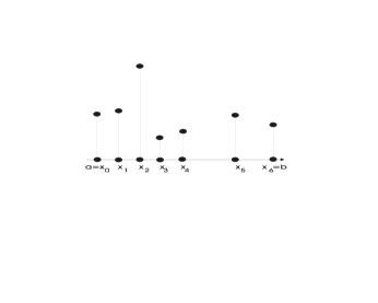
Figure 1: It is not possible to say whether this function is continuous or discrete until we have not introduced a unit of measure and a numeral system to express distances between the points

This definition emphasizes the physical principle that there does not exist an absolute continuity: it is relative with respect to the chosen instrument of observation which in our case is represented by the unit of measure $\mu$. Thus, the same set can be viewed as a continuous or not depending on the chosen unit of measure.

Example 4.1.

The set of five equidistant points

$$X_{1}=\{a,x_{1},x_{2},x_{3},x_{4}\}$$ (21)

from Fig. 1 can have the distance $d$ between the points equal to $\mbox{\char 172}^{-1}$ in a unit of measure $\mu$ and to be, therefore, continuous in $\mu$. Usage of a new unit of measure $\nu=\mbox{\char 172}^{-3}\mu$ implies that $d=\mbox{\char 172}^{2}$ in $\nu$ and the set $X_{1}$ is not continuous in $\nu$. $\Box$

Note that the introduced definition does not require that all the points from $X$ are equidistant. For instance, if in Fig. 1 for a unit measure $\mu$ the largest over the set $[a,b]_{\mathcal{S}}$ distance $x_{5}-x_{4}$ is infinitesimal, then the whole set is continuous in $\mu$.

The set $X$ is called discrete in the unit of measure $\mu$ if for all points $x\in(a,b)_{\mathcal{S}}$ it follows that the differences $x^{+}-x$ and $x-x^{-}$ from (19) expressed in units $\mu$ are not infinitesimal numbers. In our numeral system with radix grossone this means that in all the differences $x^{+}-x$ and $x-x^{-}$ negative grosspowers cannot be the largest ones. For instance, the set $X_{1}$ from (21) is discrete in the unit of measure $\nu$ from Example 4.1. Of course, it is also possible to consider intermediate cases where sets have continuous and discrete parts.

The introduced notions allow us to give the following very simple definition of a function continuous at a point. A function $f(x)$ defined over a set $[a,b]_{\mathcal{S}}$ continuous in a unit of measure $\mu$ is called continuous in the unit of measure $\mu$ at a point $x\in(a,b)_{\mathcal{S}}$ if both differences $f(x)-f(x^{+})$ and $f(x)-f(x^{-})$ are infinitesimal numbers in $\mu$, where $x^{+}$ and $x^{-}$ are from (19). For the continuity at points $a$, $b$ it is sufficient that one of these differences be infinitesimal. The notions of continuity from the left and from the right in a unit of measure $\mu$ at a point are introduced naturally. Similarly, the notions of a function discrete, discrete from the right, and discrete from the left can be defined.

The function $f(x)$ is continuous in the unit of measure $\mu$ over the set $[a,b]_{\mathcal{S}}$ if it is continuous in $\mu$ at all points of $[a,b]_{\mathcal{S}}$. Again, it becomes possible to differentiate types of continuity by taking into account values of grosspowers of infinitesimal numbers (continuity of order $\mbox{\char 172}^{-1},$ continuity of order $\mbox{\char 172}^{-2}$, etc.) and to consider functions in such units of measure that they become continuous or discrete over certain subintervals of $[a,b]$. Hereinafter, we shall often fix the unit of measure $\mu$ and write just ‘continuous function’ instead of ‘continuous function in the unit of measure $\mu$’. Let us give some examples illustrating the introduced definitions.

Example 4.2.

We start by showing that the function $f(x)=x^{2}$ is continuous over the set $X_{2}$ defined as the interval $[0,1]$ where numerals $\frac{i}{\mbox{\char 172}},0\leq i\leq\mbox{\char 172},$ are used to express its points in units $\mu$. First of all, note that the set $X_{2}$ is continuous in $\mu$ because its points are equidistant with the distance $d=\mbox{\char 172}^{-1}$. Since this function is strictly increasing, to show its continuity it is sufficient to check the difference $f(x)-f(x^{-})$ at the point $x=1$. In this case, $x^{-}=1-\mbox{\char 172}^{-1}$ and we have

$$f(1)-f(1-\mbox{\char 172}^{-1})=1-(1-\mbox{\char 172}^{-1})^{2}=2\mbox{\char 172}^{-1}(-1)\mbox{\char 172}^{-2}.$$

This number is infinitesimal, thus $f(x)=x^{2}$ is continuous over the set $X_{2}$. $\Box$

Example 4.3.

Consider the same function $f(x)=x^{2}$ over the set $X_{3}$ defined as the interval $[\mbox{\char 172}-1,\mbox{\char 172}]$ where numerals $\mbox{\char 172}-1+\frac{i}{\mbox{\char 172}},0\leq i\leq\mbox{\char 172},$ are used to express its points in units $\mu$. Analogously, the set $X_{3}$ is continuous and it is sufficient to check the difference $f(x)-f(x^{-})$ at the point $x=\mbox{\char 172}$ to show continuity of $f(x)$ over this set. In this case,

$$x^{-}=\mbox{\char 172}-1+\frac{\mbox{\char 172}-1}{\mbox{\char 172}}=\mbox{\char 172}-\mbox{\char 172}^{-1},$$

$$f(x)-f(x^{-})=f(\mbox{\char 172})-f(\mbox{\char 172}-\mbox{\char 172}^{-1})=\mbox{\char 172}^{2}-(\mbox{\char 172}-\mbox{\char 172}^{-1})^{2}=2\mbox{\char 172}^{0}(-1)\mbox{\char 172}^{-2}.$$

This number is not infinitesimal because it contains the finite part $2\mbox{\char 172}^{0}$ and, as a consequence, $f(x)=x^{2}$ is not continuous over the set $X_{3}$. $\Box$

Example 4.4.

Consider $f(x)=x^{2}$ defined over the set $X_{4}$ being the interval $[\mbox{\char 172}-1,\mbox{\char 172}]$ where numerals $\mbox{\char 172}-1+\frac{i}{\mbox{\char 172}^{2}},0\leq i\leq\mbox{\char 172}^{2},$ are used to express its points in units $\mu$. The set $X_{4}$ is continuous and we check the difference $f(x)-f(x^{-})$ at the point $x=\mbox{\char 172}$. We have

$$x^{-}=\mbox{\char 172}-1+\frac{\mbox{\char 172}^{2}-1}{\mbox{\char 172}^{2}}=\mbox{\char 172}-\mbox{\char 172}^{-2},$$

$$f(x)-f(x^{-})=f(\mbox{\char 172})-f(\mbox{\char 172}-\mbox{\char 172}^{-2})=\mbox{\char 172}^{2}-(\mbox{\char 172}-\mbox{\char 172}^{-2})^{2}=2\mbox{\char 172}^{-1}(-1)\mbox{\char 172}^{-4}.$$

Since the obtained result is infinitesimal, $f(x)=x^{2}$ is continuous over $X_{4}$. $\Box$

Let us consider now a function $f(x)$ defined by formulae over a set $X=[a,b]_{\mathcal{S}}$ so that different expressions can be used over different subintervals of $[a,b]$. The term ‘formula’ hereinafter indicates a single expression being a sequence of numerals and arithmetical operations used to evaluate $f(x)$.

Example 4.5.

The function $g(x)=2x^{2}-1,x\in[a,b]_{\mathcal{S}},$ is defined by one formula and function

$$f(x)=\left\{\begin{array}[]{ll}\max\{-14x,25x^{-1}\},&x\in[c,0)_{\mathcal{S}}\cup(0,d]_{\mathcal{S}},\\ 2x,&x=0,\end{array}\right.\hskip 14.22636ptc<0,\hskip 14.22636ptd>0,$$ (22)

is defined by three formulae, $f_{1}(x),f_{2}(x),$ and $f_{3}(x)$ where

$$\begin{array}[]{ll}f_{1}(x)=-14x,&x\in[c,0)_{\mathcal{S}},\\ f_{2}(x)=2x,&x=0,\\ f_{3}(x)=25x^{-1},&x\in(0,d]_{\mathcal{S}}.\hskip 14.22636pt\Box\end{array}$$ (23)

Consider now a function $f(x)$ defined in a neighborhood of a point $x$ as follows

$$f(\xi)=\left\{\begin{array}[]{ll}f_{1}(\xi),&x-l\leq\xi<x,\\ f_{2}(\xi),&\xi=x,\\ f_{3}(\xi),&x<\xi\leq x+r,\end{array}\right.$$ (24)

where the number $l$ is any number such that the same formula $f_{1}(\xi)$ is used to define $f(\xi)$ at all points $\xi$ such that $x-l\leq\xi<x$. Analogously, the number $r$ is any number such that the same formula $f_{3}(\xi)$ is used to define $f(\xi)$ at all points $\xi$ such that $x<\xi\leq x+r$. Of course, as a particular case it is possible that the same formula is used to define $f(\xi)$ over the interval $[x-l,x+r]$, i.e.,

$$f(\xi)=f_{1}(\xi)=f_{2}(\xi)=f_{3}(\xi),\hskip 14.22636pt\xi\in[x-l,x+r].$$ (25)

It is also possible that (25) does not hold but formulae $f_{1}(\xi)$ and $f_{3}(\xi)$ are defined at the point $x$ and are such that at this point they return the same value, i.e.,

$$f_{1}(x)=f_{2}(x)=f_{3}(x).$$ (26)

If condition (26) holds, we say that function $f(x)$ has continuous formulae at the point $x$. Of course, in the general case, formulae $f_{1}(\xi),f_{2}(\xi),$ and $f_{3}(\xi)$ can be or cannot be defined out of the respective intervals from (24). In cases where condition (26) is not satisfied we say that function $f(x)$ has discontinuous formulae at the point $x$. Definitions of functions having formulae which are continuous or discontinuous from the left and from the right are introduced naturally. Let us give an example showing that the introduced definition can also be easily used for functions assuming infinitesimal and infinite values.

Example 4.6.

Let us study the following function that at infinity, in the neighborhood of the point $x=\mbox{\char 172}$, assumes infinitesimal values

$$f(x)=\left\{\begin{array}[]{ll}\mbox{\char 172}^{-1}+5(x-\mbox{\char 172}),&x\neq\mbox{\char 172},\\ \mbox{\char 172}^{-2},&x=\mbox{\char 172}.\end{array}\right.$$ (27)

By using designations (24) we have

$$f(\xi)=\left\{\begin{array}[]{ll}f_{1}(\xi)=\mbox{\char 172}^{-1}+5(x-\mbox{\char 172}),&\xi<\mbox{\char 172},\\ f_{2}(\xi)=\mbox{\char 172}^{-2},&\xi=\mbox{\char 172},\\ f_{3}(\xi)=\mbox{\char 172}^{-1}+5(x-\mbox{\char 172}),&\xi>\mbox{\char 172},\end{array}\right.$$

Since

$$f_{1}(\mbox{\char 172})=f_{3}(\mbox{\char 172})=\mbox{\char 172}^{-1}\neq f_{2}(\mbox{\char 172})=\mbox{\char 172}^{-2},$$

we conclude that the function (27) has discontinuous formulae at the point $x=\mbox{\char 172}$. It is remarkable that we were able to establish this easily in spite of the fact that all three values, $f_{1}(\mbox{\char 172}),f_{2}(\mbox{\char 172}),$ and $f_{3}(\mbox{\char 172})$ were infinitesimal and were evaluated at infinity. Analogously, the function (22) has continuous formulae at the point $x=0$ from the left and discontinuous from the right. $\Box$

Example 4.7.

Let us study the following function

$$f(x)=\left\{\begin{array}[]{ll}\mbox{\char 172}^{3}+\frac{x^{2}-1}{x-1},&x\neq 1,\\ a,&x=1,\end{array}\right.$$ (28)

at the point $x=1$. By using designations (24) and the fact that for $x\neq 1$ it follows $\frac{x^{2}-1}{x-1}=x+1$, from where we have

$$f(\xi)=\left\{\begin{array}[]{ll}f_{1}(\xi)=\mbox{\char 172}^{3}+\xi+1,&\xi<1,\\ f_{2}(\xi)=a,&\xi=1,\\ f_{3}(\xi)=\mbox{\char 172}^{3}+\xi+1,&\xi>1,\end{array}\right.$$

Since

$$f_{1}(1)=f_{3}(1)=\mbox{\char 172}^{3}+2,\hskip 28.45274ptf_{2}(1)=a,$$

we obtain that if $a=\mbox{\char 172}^{3}+2$, then the function (28) has continuous formulae at the point $x=1$, otherwise it has discontinuous formulae at this point. Note, that even if $a=\mbox{\char 172}^{3}+2+\varepsilon$, where $\varepsilon$ is an infinitesimal number (remind that all infinitesimals are not equal to zero), we establish easily that the function has discontinuous formulae in spite of the fact that both numbers, $\mbox{\char 172}^{3}+2$ and $a$, are infinite. $\Box$

Similarly to the existence of numerals that cannot be expressed through other numerals, in mathematics there exist functions that cannot be expressed as a sequence of numerals and arithmetical operations because (again similarly to numerals) they are introduced through their properties. Let us consider, for example, the function $f(x)=\sin(x)$. It can be immediately seen that it does not satisfy the traditional definition of a function (see the corresponding discussion in page 4). We know well its codomain but the story becomes more difficult with its domain and impossible with the relation that it is necessary to establish to obtain $f(x)$ when a value for $x$ is given. In fact, we know precisely the value of $\sin(x)$ only at certain points $x$; for other points the value of $\sin(x)$ are measured (as a result, errors are introduced) or approximated (again errors are introduced), and, finally, as it has been already mentioned, not all points $x$ can be expressed by known numeral systems.

However, traditional approaches allow us to confirm its continuity (which is clear due to the physical way it has been introduced) also from positions of general definitions of continuity both in standard and non-standard Analysis. Let us show that, in spite of the fact that we do not know a complete formula for calculating $\sin(x)$, the new approach also allows us to show that $\sin(x)$ is a function with continuous formulae. This can be done by using partial information about the structure of the formula of $\sin(x)$ by appealing to the same geometrical ideas that are used in the traditional proof of continuity of $\sin(x)$ (cf. [6]).

Theorem 4.1.

The function $f(x)=\sin(x)$ has continuous formulae.

Proof. Let us first show that $\sin(x)$ has continuous formulae at $x=0$. By using designations (25) and well-known geometrical considerations we can write for $f_{1}(\xi),f_{3}(\xi)$ and $x=0$ the following relations

$$\xi<f_{1}(\xi)<0,\hskip 14.22636pt-\frac{\pi}{2}<\xi<0,$$ (29)

$$0<f_{3}(\xi)<\xi,\hskip 14.22636pt0<\xi<\frac{\pi}{2}.$$ (30)

Thus, even though we are not able to calculate $f_{1}(\xi)$ and $f_{3}(\xi)$ at points $\xi\neq 0$, we can use the estimates (29) and (30) from where we obtain $f_{1}(0)=f_{3}(0)=0$ because the estimate $\xi$ being at the left part of (29) and at the right part of (30) can be evaluated at the point $\xi=0$. It then follows from the obvious fact $f_{2}(\xi)=0$ that $\sin(x)$ has continuous formulae at $x=0$. By a complete analogy, the fact that the function $f(x)=\cos(x)$ has continuous formulae at $x=0$ can be proved.

If we represent now the point $\xi$ in the form $\xi=x+\zeta$ then we can write

$$\sin(x+\zeta)=\sin(x)\cos(\zeta)+\cos(x)\sin(\zeta).$$

Inasmuch as both $\sin(x)$ and $\cos(x)$ have continuous formulae at the point $x=0$, it follows that at the point $\xi=x$ we have

$$f_{1}(x)=f_{3}(x)=\sin(x+0)=\sin(x)\cos(0)+\cos(x)\sin(0)=\sin(x).$$

This fact concludes the proof because obviously $f_{2}(x)=\sin(x)$, too. $\Box$

Corollary 4.1.

The function $f(x)=\cos(x)$ has continuous formulae.

Proof. The fact is a straightforward consequence of the theorem. $\Box$

To conclude this section we emphasize that functions having continuous formulae at a point can be continuous or discrete at this point depending on the chosen unit of measure. Analogously, functions having discontinuous formulae at a point can be continuous or discrete at this point again depending on the chosen unit of measure. The notion of continuity of a function depends on the chosen unit of measure and numeral system $\mathcal{S}$ and it can be used for functions defined by formulae, computer procedures, tables, etc. In contrast, the notion of a function having continuous formulae works only for functions defined by formulae and does not depend on units of measure or numeral systems chosen to express its domain. It is related only to properties of formulae and does not depend on the domain at all. Note that we have established the facts of continuity or discontinuity of formulae in Theorem 4.1 and Examples 4.6, 4.7 without indicating domains of the considered functions.

5 Differential calculus

In this section, the notions of the first derivative and subdifferential are introduced. Both concepts are defined without usage of limits and for functions assuming finite, infinite, and infinitesimal values. We first give all the definitions and then illustrate them by a series of examples. Special attention (as in the entire paper) is paid to the computational issues and their relations to the introduced definitions.

We shall call the following two expressions, $f^{-}(x,l)$ and $f^{+}(x,r)$, that are obtained by isolating the multipliers $l$ and $r$ in the left and the right differences $f_{1}(x)-f_{1}(x-l)$ and $f_{3}(x+r)-f_{3}(x)$, respectively, the left and the right relative differences for $f(x)$ at a point $x$:

$$f_{1}(x)-f_{1}(x-l)=l\cdot f^{-}(x,l),\hskip 28.45274ptl\geq 0,$$ (31)

$$f_{3}(x+r)-f_{3}(x)=r\cdot f^{+}(x,r),\hskip 28.45274ptr\geq 0.$$ (32)

In the introduced definitions (examples will be given soon) it is not required that the numbers $l$ and $r$ from (24) tend to zero – they can be finite or even infinite. Their boundaries are determined by formulae $f_{1}(\xi),f_{2}(\xi),$ and $f_{3}(\xi)$ defining $f(\xi)$. Note that the value of $f(\xi)$ at the point $\xi=x$ is defined by formula $f_{2}(\xi)$ which is not used in (31) and (32).

If for $\xi=x$ formula $f^{-}(\xi,l)$ is defined at $l=0$ and/or $f^{+}(\xi,r)$ is defined at $r=0$, then functions

$$f^{-}(x)=f^{-}(x,0),\hskip 28.45274ptf^{+}(x)=f^{+}(x,0),$$ (33)

are called left and right derivatives at the point $x$, respectively. We can also introduce functions

$$\tilde{f}^{-}(x,l)=f^{-}(x,l)-f^{-}(x),$$ (34)

$$\tilde{f}^{+}(x,r)=f^{+}(x,r)-f^{+}(x).$$ (35)

Note that obtained formulae give us possibility to evaluate $f^{-}(x,l),\tilde{f}^{-}(x,l)$ and $f^{+}(x,r),\tilde{f}^{+}(x,r)$ at any points

$$x\in[a,b],\hskip 28.45274ptx-l\in[a,b],\hskip 28.45274ptx+r\in[a,b],$$ (36)

where formulae $f_{1}(\xi),f_{2}(\xi),$ and $f_{3}(\xi)$ are used but we are able to calculate them only at those points that can be expressed in our numeral system $\mathcal{S}$, i.e., at the points $x,x-l$, and $x+r$ such that

$$x\in[a,b]_{\mathcal{S}},\hskip 28.45274ptx-l\in[a,b]_{\mathcal{S}},\hskip 28.45274ptx+r\in[a,b]_{\mathcal{S}}.$$ (37)

Geometrically, $f^{-}(x,l)$ is the slope of the straight line passing through the points $(x-l,f_{1}(x-l))$ and $(x,f_{1}(x))$. Analogously, $f^{+}(x,r)$ is the slope of the straight line passing through the points $(x,f_{3}(x))$ and $(x+r,f_{3}(x+r))$. The left derivative, $f^{-}(x)$, can be viewed as the slope of the line constructed at the point $(x,f_{1}(x))$ and $\tilde{f}^{-}(x,l)$ is the difference between the slopes of this line and that passing through the points $(x-l,f_{1}(x-l))$ and $(x,f_{1}(x))$ with the slope $f^{-}(x,l)$. Analogously, $f^{+}(x)$ can be viewed as the slope of the line constructed at the point $(x,f_{3}(x))$ and $\tilde{f}^{+}(x,r)$ is the difference between the slopes of this line and that passing through the points $(x,f_{3}(x))$ and $(x+r,f_{3}(x+r))$ with the slope $f^{+}(x,r)$.

Thus, the left derivative describes the behavior of $f(\xi)$ on the left of the point $x$ and the right derivative on its right. Both of them are independent of the value $f_{2}(x)$ at the point $x$.

Below we introduce the notions of derivative and derivatives interval and give their geometrical interpretation in dependence on the mutual positions of the two lines passing through the points $(x,f_{1}(x))$ and $(x,f_{3}(x))$ with the slopes $f^{-}(x)$ and $f^{+}(x)$, respectively. We suppose that the right and the left derivatives exist and function $f(x)$ has continuous formulae at the point $x$. The latter supposition means that the points $(x,f_{1}(x)),(x,f_{2}(x)),$ and $(x,f_{3}(x))$ coincide.

If at a point $x$ formulae $f^{-}(x)$ and $f^{+}(x)$ can be written down in the same form then the following function

$$f^{\prime}(x)=f^{-}(x)=f^{+}(x)$$ (38)

is called derivative of $f(x)$ at the point $x$ and function $f(x)$ is called antiderivative of $f^{\prime}(x)$ at this point (this terminology will be used for $f(x)$ in the two following cases too).

If at a point $\tau\in[a,b]_{\mathcal{S}}$ we obtain that $f^{-}(\tau)=f^{+}(\tau)$ but formulae $f^{-}(x)$ and $f^{+}(x)$ cannot be written down in the same form, then the value $f^{-}(\tau)$ is called derivative of $f(x)$ at the point $\tau$ and formulae to express derivative $f^{\prime}(\tau)$ should be chosen in concordance with the choice of the formula used to express antiderivative $f(x)$. Geometrically, this case and the previous one have the same meaning and $f^{\prime}(\tau)$ is the slope of the straight line passing through the points $(\tau,f(\tau))$ and tangent to the graph of the function $f(x)$ at the point $\tau$.

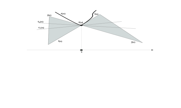
Figure 2: Two tangent lines, $f_{1}(x)$ and $f_{2}(x)$, passing through the point $(\tau,f(\tau))$ and having slopes equal to two derivatives $f^{\prime}_{1}$ and $f^{\prime}_{2}$ from the derivatives interval $[\underline{f}(\tau),\overline{f}(\tau)]$ (shown in grey color) of a function $f(x)$ at a point $\tau$

If at a point $\tau\in[a,b]_{\mathcal{S}}$ we obtain that $f^{-}(\tau)\neq f^{+}(\tau)$ then the interval $[\underline{f}(\tau),\overline{f}(\tau)]$ is called derivatives interval of $f(x)$ at the point $\tau$ where

$$\underline{f}(\tau)=\min\{f^{-}(\tau),f^{+}(\tau)\},$$ (39)

$$\overline{f}(\tau)=\max\{f^{-}(\tau),f^{+}(\tau)\}.$$ (40)

Geometrically, the derivatives interval contains slopes of all lines tangent to the graph of the function at the point $\tau$. In this case, the user chooses from the derivatives interval that derivative which fits better his/her requirements (accuracy, type of used algorithms, etc.) and works with it (a similar situation takes place when one deals with subdifferentials (see [4])). This case is illustrated in Fig. 2 were two tangent lines using derivatives, $f^{\prime}_{1}$ and $f^{\prime}_{2}$, from the interval $[\underline{f}(\tau),\overline{f}(\tau)]$ are shown.

Let us make a few comments. First of all, it is important to notice that in the traditional approach the derivative (if it exists) is a finite number and it can be defined only for continuous functions. In our terminology, it can be finite, infinite, or infinitesimal and its existence does not depend on continuity of the function but on continuity of formulae. The derivatives interval can exist for discrete and continuous functions defined over continuous sets, for functions defined over discrete sets, and for functions having infinite or infinitesimal values defined over sets having infinitesimal or infinite boundaries.

The derivative (or derivatives interval) can be possibly defined if the function under consideration has been introduced by formulae and it cannot be defined if the function has been introduced by a computer procedure or by a table. Thus, we emphasize that just the fact of presence of an analytical expression of $f(x)$ allows us to find its derivatives interval.

When a function $f(x)$ is defined only by a computer procedure and its analytical expressions are unknown, we cannot define derivatives. We can only try to obtain a numerical approximation without any estimate of its accuracy. For a point $x\in[a,b]_{\mathcal{S}}$ we define the interval $[\underline{f}(x)_{\mathcal{S}},\overline{f}(x)_{\mathcal{S}}]$ called numerical derivatives interval of $f(x)$ at the point $x$ expressed in the system $\mathcal{S}$ where

$$\underline{f}(x)_{\mathcal{S}}=\min\{f^{-}(x,x^{-}),f^{+}(x,x^{+})\},$$ (41)

$$\overline{f}(x)_{\mathcal{S}}=\max\{f^{-}(x,x^{-}),f^{+}(x,x^{+})\},$$ (42)

and the points $x^{-},x^{+}$ are from (19). Each element $f^{\prime}(x)\in[\underline{f}(x)_{\mathcal{S}},\overline{f}(x)_{\mathcal{S}}]$ is called numerical derivative of $f(x)$ at the point $x$ expressed in $\mathcal{S}$.

Numerical derivatives interval can be useful also when formulae of $f(x)$ are known. For example, if we have obtained that at a point $x\in[a,b]_{\mathcal{S}}$ there exists the unique value $f^{\prime}(x)$ and $f^{\prime}(x)\notin[\underline{f}(x)_{\mathcal{S}},\overline{f}(x)_{\mathcal{S}}]$ then this means that the chosen numeral system $\mathcal{S}$ is too rude to be used for presentation of $f(x)$. This situation is illustrated in Fig. 3 where points $x,x^{-},$ and $x^{+}$ expressed in $\mathcal{S}$ are shown by big dots. Small dots show the behavior of $f(x)$ expressed in a more powerful numeral system. It can be clearly seen from Fig. 3 that $f^{\prime}(x)\notin[\underline{f}(x)_{\mathcal{S}},\overline{f}(x)_{\mathcal{S}}]$.

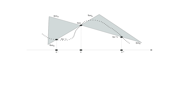
Figure 3: The numeral system $\mathcal{S}$ able to express only points $x,x^{-},$ and $x^{+}$ is too crude to present adequately the behavior of $f(x)$

Note also that relaxed definitions of derivative and derivatives interval can be also given by asking, instead of (26), satisfaction of $f_{1}(\tau)=f_{3}(\tau)$ only (therefore, $f_{1}(\tau)\neq f_{2}(\tau)$) can occur). For this case, the same derivative interval is obtained but it contains slopes of lines tangent to the graph of the following function

$$\hat{f}(x)=\left\{\begin{array}[]{ll}f(x),&x\neq\tau,\\ f_{1}(\tau),&x=\tau.\end{array}\right.$$

Example 5.1.

Consider again the function $f(x)=x^{2}$ at a point $x$ and calculate its left and right differences. Condition (25) holds for this function everywhere and, therefore, it has continuous formulae at any point $x$. Then

$$f_{1}(x)-f_{1}(x-l)=x^{2}-(x-l)^{2}=2xl-l^{2}=l(2x-l)$$

and due to (31) it follows

$$f^{-}(x,l)=2x-l.$$

Analogously, from (32) we obtain

$$f_{3}(x+r)-f_{3}(x)=(x+r)^{2}-x^{2}=2xr+r^{2}=r(2x+r),$$

$$f^{+}(x,r)=2x+r.$$

Since both functions $f^{-}(x)=f^{-}(x,0)$ and $f^{+}(x)=f^{+}(x,0)$ exist and

$$f^{-}(x)=f^{+}(x)=2x,$$

the function $f(x)=x^{2}$ has the unique derivative $f^{\prime}(x)=2x$ at any point (finite, infinite, or infinitesimal) expressible in the chosen numeral system $\mathcal{S}$. For instance, if $x=\mbox{\char 172}$ then we obtain infinite values $f(\mbox{\char 172})=\mbox{\char 172}^{2}$ and $f^{\prime}(\mbox{\char 172})=2\mbox{\char 172}$. For infinitesimal $x=\mbox{\char 172}^{-1}$ we have infinitesimal values $f(\mbox{\char 172}^{-1})=\mbox{\char 172}^{-2}$ and $f^{\prime}(\mbox{\char 172}^{-1})=2\mbox{\char 172}^{-1}$. $\Box$

It is important to emphasize that the introduced definitions also work for functions including infinite and infinitesimal values in their formulae. For instance, it follows immediately from the above consideration in Example 5.1 that functions $g_{1}(x)=\mbox{\char 172}^{-1}x^{2}$ and $g_{2}(x)=\mbox{\char 172}x^{2}$ have derivatives $g_{1}^{\prime}(x)=2\mbox{\char 172}^{-1}x$ and $g_{2}^{\prime}(x)=2\mbox{\char 172}x$, respectively.

Inasmuch as the case where at a point $\tau\in[a,b]_{\mathcal{S}}$ we obtain that $f^{-}(\tau)=f^{+}(\tau)$ but formulae $f^{-}(x)$ and $f^{+}(x)$ cannot be written down in the same form is a simple consequence of the previous case, we give an example of the situation where at a point $\tau\in[a,b]_{\mathcal{S}}$ we obtain that $f^{-}(\tau)\neq f^{+}(\tau)$.

Example 5.2.

Let us consider the following function

$$f(x)=\left\{\begin{array}[]{ll}-x,&x\leq 0,\\ x+C,&x>0,\end{array}\right.$$ (43)

where $C$ is a constant. Then to define the function completely it is necessary to choose an interval $[a,b]$ and a numeral system $\mathcal{S}$.

Suppose now that the chosen numeral system, $\mathcal{S}$, is such that the point $x=0$ does not belong to $[a,b]_{\mathcal{S}}$. Then we immediately obtain from (31) – (33), (38) that at any point $x\in[a,b]_{\mathcal{S}}$ the function has a unique derivative and

$$f^{\prime}(x)=\left\{\begin{array}[]{rl}-1,&x<0,\\ 1,&x>0.\end{array}\right.$$ (44)

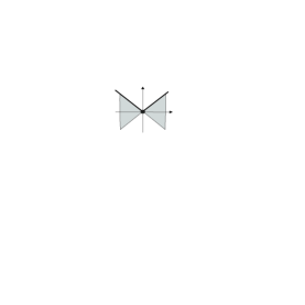
Figure 4: Derivatives interval (shown in grey color) for the function defined by formula (43) with $C=0$.

If the chosen numeral system, $\mathcal{S}$, is such that the point $x=0$ belongs to $[a,b]_{\mathcal{S}}$ then (44) is also true for $x\neq 0$ and we should verify the existence of the derivative or derivatives interval for $x=0$. It follows from (31) and (33) that at this point the left derivative exists and is calculated as follows

$$f_{1}(x)-f_{1}(x-l)=-x-(-(x-l))=l\cdot(-1),$$

$$f^{-}(x,l)=-1,\hskip 28.45274ptf^{-}(x)=f^{-}(x,0)=-1.$$

The right derivative is obtained analogously from (32) and (33)

$$f_{3}(x+r)-f_{3}(x)=x+C+r-(x+C)=r\cdot 1,$$

$$f^{+}(x,r)=1,\hskip 28.45274ptf^{+}(x)=f^{+}(x,0)=1.$$

However, $f(x)$ has continuous formulae at the point $x=0$ only for $C=0$. Thus, only in this case function $f(x)$ defined by (43) has the derivatives interval $[-1,1]$ at the point $x=0$. This situation is illustrated in Fig. 4.

By a complete analogy it is possible to show that functions

$$\begin{array}[]{cc}\hat{f}(x)=\left\{\begin{array}[]{ll}-2\mbox{\char 172}x,&x\leq 0,\\ 3\mbox{\char 172}x^{2},&x>0,\end{array}\right.&\hskip 28.45274pt\tilde{f}(x)=\left\{\begin{array}[]{ll}-4\mbox{\char 172}^{-1.6}x,&x\leq 0,\\ 5\mbox{\char 172}^{-28}x,&x>0,\end{array}\right.\end{array}$$

have at the point $x=0$ derivatives intervals $[-2\mbox{\char 172},0]$ and $[-4\mbox{\char 172}^{-1.6},5\mbox{\char 172}^{-28}]$, respectively. The first of them is infinite and the second infinitesimal. $\Box$

Let us find now the derivative of the function $f(x)=\sin(x)$. As in standard and non-standard analysis, this is done by appealing to geometrical arguments.

Lemma 5.1.

There exists a function $g(x)$ such that the function $f(x)=\sin(x)$ can be represented by the following formula: $\sin(x)=x\cdot g(x),$ where $g(0)=1$.

Proof. Let us consider a function $d(x)=\frac{\sin(x)}{x}$ and study it on the right from the point $x=0$, i.e., in the form $d_{3}(\xi)$ from (24) for $\xi>0$ (the function $d_{1}(\xi)$ is investigated by a complete analogy). It is easy to show from geometrical considerations (see [6]) that

$$1<\frac{\xi}{\sin(\xi)}<\frac{1}{\cos(\xi)},\hskip 28.45274pt0<\xi<\frac{\pi}{2}.$$

Inasmuch as $\xi\neq 0$, it follows from these estimates that

$$\cos(\xi)<\frac{\sin(\xi)}{\xi}<1,\hskip 28.45274pt0<\xi<\frac{\pi}{2},$$

and, therefore,

$$\cos(\xi)<d_{3}(\xi)<1,\hskip 28.45274pt0<\xi<\frac{\pi}{2},$$

Due to Corollary 4.1, the function $\cos(x)$ has continuous formulae and $\cos(0)=1$. As a consequence, we obtain $d_{3}(0)=1$. Since the formula $d(\xi)=\frac{\sin(\xi)}{\xi}$ has $\xi$ in the denominator, the only possibility to execute the reduction in the formula $d_{3}(\xi)$ leading to the result $d_{3}(0)=1$ consists of the existence of the function $g(\xi)$ such that $d_{3}(\xi)=\frac{\xi\cdot g(\xi)}{\xi}=g(\xi)$. The fact that $\sin(x)$ has continuous formulae concludes the proof. $\Box$

This lemma illustrates again our methodological point of view expressed in Postulate 2. The formula $d(x)=\frac{\sin(x)}{x}$ has zero in the denominator when $x=0$. In contrast, the function $g(x)$ is defined also for $x=0$ in spite of the fact that they describe the same mathematical object. The difficulties we have in $d(x)$ have been introduced by inadequate mathematical instruments used to describe the object, particularly, by the fact that the precise formula for $\sin(x)$ is unknown. Analogously, if we rewrite the constant function $c(x)=1$ in the form $m(x)=x\cdot\frac{1}{x}$ we obtain the same effect. Introduction of the designations (24) allows us to monitor this situation easily.

Theorem 5.1.

The derivative of the function $f(x)=\sin(x)$ is $f^{\prime}(x)=\cos(x)$.

Proof. Let us calculate the right relative difference, $f^{+}(x,r)$, from (32) for $f(x)=\sin(x)$ at a point $x$ as follows

$$f_{3}(x+r)-f_{3}(x)=\sin(x+r)-\sin(x)=\sin(x)\cos(r)+\cos(x)\sin(r)-\sin(x).$$

By using the trigonometric identity

$$\cos(x)=1-2\sin^{2}(0.5x)$$

and Lemma 5.1 we obtain

$$f_{3}(x+r)-f_{3}(x)=\sin(x)(\cos(r)-1)+\cos(x)\sin(r)=$$

$$\sin(r)\cos(x)-2\sin^{2}(0.5r)\sin(x)=r\cdot g(r)\cos(x)-0.5r^{2}\cdot g(0.5r)^{2}\sin(x)=$$

$$r\big{(}g(r)\cos(x)-0.5r\cdot g(0.5r)^{2}\sin(x)\big{)}.$$

Thus, we have that the right relative difference

$$f^{+}(x,r)=g(r)\cos(x)-0.5r\cdot g(0.5r)^{2}\sin(x).$$

By recalling again Lemma 5.1 we obtain from this formula that

$$f^{+}(x)=f^{+}(x,0)=g(0)\cos(x)=1\cdot\cos(x)=\cos(x).$$

By a complete analogy (see (31)) we obtain that $f^{-}(x)=\cos(x)$, too. Due to the introduced definition of the derivative (see (31)–(33), (38)), it follows from the fact $f^{+}(x)=f^{-}(x)$ that $f^{\prime}(x)=\cos(x)$. $\Box$

We conclude this section by an example showing the usage of derivatives for calculating sums with an infinite number of items. Recall that due to Postulate 3 and since we have infinite numbers that can be written explicitly, we cannot define a function in the form $f(x)=\sum_{i=0}^{\infty}a_{i}(x)$. It is necessary to indicate explicitly an infinite number, $n$, of items in the sum $f(x)=\sum_{i=0}^{n}a_{i}(x)$ and, obviously, two different infinite numbers, $n=n_{1}$ and $n=n_{2}$, will define two different functions.

Example 5.3.

Let us consider an infinite number $n$ and the following function

$$f(x)=\sum_{i=0}^{n}x^{i}=1+x+x^{2}+\ldots+x^{n},$$ (45)

where $x\neq 1$ can be finite, infinite or infinitesimal. By derivating (45) we obtain

$$f^{\prime}(x)=\sum_{i=1}^{n}ix^{i-1}=1+2x+3x^{2}+\ldots+nx^{n-1}.$$ (46)

However, it follows from (12) and (13) that

$$f(x)=\frac{1-x^{n+1}}{1-x}.$$ (47)

By derivating (47) we have that

$$f^{\prime}(x)=\frac{1+nx^{n+1}-(n+1)x^{n}}{(1-x)^{2}}.$$ (48)

Thus, we can conclude that for finite and infinite $n$ and for finite, infinite or infinitesimal $x\neq 1$ it follows

$$\frac{1+nx^{n+1}-(n+1)x^{n}}{(1-x)^{2}}=\sum_{i=1}^{n}ix^{i-1}=1+2x+3x^{2}+\ldots+nx^{n-1},$$ (49)

whereas the traditional analysis uses just the following formula

$$\frac{1}{(1-x)^{2}}=\sum_{i=0}^{\infty}ix^{i-1}=1+2x+3x^{2}+\ldots,$$

that is able to provide a result only if for any infinite $n$ there exists a finite approximation of (49) and it is used only for finite $x,$ $-1<x<1$. $\Box$

6 Conclusion

In this paper, a new applied methodology to Calculus has been proposed. It has been emphasized that the philosophical triad – the researcher, the object of investigation, and tools used to observe the object – existing in such natural sciences as Physics and Chemistry exists in Mathematics, too. In natural sciences, the instrument used to observe the object influences results of observations. The same happens in Mathematics studying numbers and objects that can be constructed by using numbers. Thus, numeral systems used to express numbers are instruments of observations used by mathematicians. The usage of powerful numeral systems gives the possibility of obtaining more precise results in Mathematics in the same way as usage of a good microscope gives the possibility to obtain more precise results in Physics.

A brief introduction to a unified theory of continuous and discrete functions has been given for functions that can assume finite, infinite, and infinitesimal values over finite, infinite, and infinitesimal domains. This theory allows one to work with derivatives and subdifferentials that can assume finite, infinite, and infinitesimal values, as well. It has been shown that the expressed point of view on Calculus allows one to avoid contrapositions of the previous approaches (finite quantities versus infinite, standard analysis versus non-standard, continuous analysis versus discrete, numerical analysis versus pure) and to create a unique framework for Calculus having a simple and intuitive structure. It is important to emphasize that the new approach has its own computational tool – the Infinity Computer – able to execute numerical computations with finite, infinite, and infinitesimal quantities.

References

- [1] V. Benci and M. Di Nasso, Numerosities of labeled sets: a new way of counting, Advances in Mathematics 173 (2003), 50–67.
- [2] G. Cantor, Contributions to the founding of the theory of transfinite numbers, Dover Publications, New York, 1955.
- [3] A.L. Cauchy, Le calcul infinitésimal, Paris, 1823.
- [4] F.H. Clarke, Optimization and nonsmooth analysis, Wiley, New York, 1983.
- [5] J.H. Conway and R.K. Guy, The book of numbers, Springer-Verlag, New York, 1996.
- [6] R. Courant and F. John, Introduction to calculus and analysis I, Springer-Verlag, New York, 1999.
- [7] J. d’Alembert, Différentiel, Encyclopédie, ou dictionnaire raisonné des sciences, des arts et des métiers 4 (1754).
- [8] P. Gordon, Numerical cognition without words: Evidence from Amazonia, Science 306 (2004), no. 15 October, 496–499.
- [9] G.W. Leibniz and J.M. Child, The early mathematical manuscripts of Leibniz, Dover Publications, New York, 2005.
- [10] I. Newton, Method of fluxions, 1671.
- [11] H.-O. Peitgen, H. Jürgens, and D. Saupe, Chaos and fractals, Springer-Verlag, New York, 1992.
- [12] P. Pica, C. Lemer, V. Izard, and S. Dehaene, Exact and approximate arithmetic in an amazonian indigene group, Science 306 (2004), no. 15 October, 499–503.
- [13] A. Robinson, Non-standard analysis, Princeton Univ. Press, Princeton, 1996.
- [14] Ya.D. Sergeyev, Arithmetic of infinity, Edizioni Orizzonti Meridionali, CS, 2003.
- [15] Ya.D. Sergeyev, Computer system for storing infinite, infinitesimal, and finite quantities and executing arithmetical operations with them, patent application 08.03.04, 2004.
- [16] , http://www.theinfinitycomputer.com, 2004.
- [17] , Mathematical foundations of the Infinity Computer, Annales UMCS Informatica AI 4 (2006), 20–33.
- [18] , Blinking fractals and their quantitative analysis using infinite and infinitesimal numbers, Chaos, Solitons Fractals 33(1) (2007), 50–75.
- [19] , Measuring fractals by infinite and infinitesimal numbers, Mathematical Methods, Physical Methods Simulation Science and Technology 1(1) (2008), 217–237.
- [20] , Modelling season changes in the infinite processes of growth of biological systems, Transactions on Applied Mathematics and Nonlinear Models (2008), (to appear).
- [21] , A new applied approach for executing computations with infinite and infinitesimal quantities, Informatica 19(4) (2008), 567–596.
- [22] , Numerical computations and mathematical modelling with infinite and infinitesimal numbers, Journal of Applied Mathematics and Computing 29 (2009), 177–195.
- [23] J. Wallis, Arithmetica infinitorum, 1656.