Measuring the vulnerability of the Uruguayan population to vector-borne diseases via spatially hierarchical factor models

Abstract

We propose a model-based vulnerability index of the population from Uruguay to vector-borne diseases. We have available measurements of a set of variables in the census tract level of the 19 Departmental capitals of Uruguay. In particular, we propose an index that combines different sources of information via a set of micro-environmental indicators and geographical location in the country. Our index is based on a new class of spatially hierarchical factor models that explicitly account for the different levels of hierarchy in the country, such as census tracts within the city level, and cities in the country level. We compare our approach with that obtained when data are aggregated in the city level. We show that our proposal outperforms current and standard approaches, which fail to properly account for discrepancies in the region sizes, for example, number of census tracts. We also show that data aggregation can seriously affect the estimation of the cities vulnerability rankings under benchmark models.

, , , and

t1Supported by the University of Chicago Booth School of Business. t2Supported in part by grants from CNPq and FAPERJ. t3Supported by a Postdoctoral fellowship from FAPERJ.

1 Vulnerability assessment

Vulnerability can be defined by a set of characteristics of a person (or a group of people), which determines her (or their) ability to anticipate, survive, resist and recover from the impact of a dangerous situation [Blaikie et al. (1994)]. In addition, Clark et al. (2000) mention that “questions about vulnerability of social and ecological systems are emerging as a central focus of policy-driven assessments of global environmental risks in arenas as different as the ongoing work of the Intergovernmental Panel on Climate Change, the World Economic Forum, and the World Food Programme.” They continue by saying that “vulnerability is emerging as a multidimensional concept involving at least (i) exposure: the degree to which a human group or ecosystem comes into contact with particular stresses; (ii) sensitivity: the degree to which an exposure unit is affected by exposure to any set of stresses; and (iii) resilience: the ability of the exposure unit to resist or recover from the damage associated with the convergence of multiple stresses.” Adger (2006) provides a recent review on analytical approaches to vulnerability to environmental changes. Eakin and Luers (2006) discuss new insights into the conceptualization of the vulnerability of social-environmental systems. They argue that a diversity of approaches to studying vulnerability is necessary in order to address the full complexity of the concept.

1.1 Vulnerability to vector-borne diseases

In this paper we construct a micro-environmental index that describes the vulnerability of the population of Uruguay to vector-borne diseases, both at the city level, as well as their census-tracts. We measure vulnerability by combining the information from a set of indicators that capture the average social profile of the population, and the average environmental condition experienced by households, in a given census tract of a city. The very nature of our spatial model (see Section 2) allows the assessment of the vulnerability index for the 19 cities in the study (see Section 1.2), as well as other Uruguayan cities not included in the study.

In general, approaches that characterize the vulnerability of human population to vector-borne diseases present problems and limitations. Some approaches consider poverty as a determinant indicator, while others consider climate conditions of key importance to measure vulnerability [Hahn, Riederer and Foster (2009)]. The approaches that assign special importance to poverty, do so in a classical sense, that is, they are related to pointing limitations in the availability of financial resources [Beltrami (2008)]. Unarguably, poverty is an important component of the quality of a person’s life. Nonetheless, the assumption that poverty can solely define a vulnerability index to vector-borne diseases is a strong and unrealistic one. Adger (2006) points that many authors [e.g., Sen (1981) and Sarewitz, Pielke and Keykhah (2003)] have argued that vulnerability is not the same as poverty. He goes on mentioning that a vulnerability measure needs to incorporate well-being defined broadly.

An alternative approach is to consider climate characteristics at global, regional and local scales. These refer to ecological conditions suitable for the development of the vector, focusing the analysis on the probability of presence of the vector in the area, and on its ability to increase its population in some season of the year [Lyth, Holbrook and Beggs (2005)]. These approaches are closely related to the knowledge of the potential conditions of the development of the vector under certain conditions, for example, climate variability, changes in land use and environmental changes, rather than people’s vulnerability to the presence of the vector [van Leishout et al. (2004)].

There are in the literature different approaches to assess vulnerability. For example, Cutter, Boruff and Shirley (2003) make use of socioeconomic and demographic data to construct an index of social vulnerability to environmental hazards (denoted SoVI) for the United States. Their index is based on a linear combination of factors obtained through the use of 42 variables observed for all 3,141 U.S. counties. Schmidtlein et al. (2008) analyze the SoVI of Cutter, Boruff and Shirley (2003) and discuss its sensitivity to the geographic context under which the analysis is performed. Rygel, O’Sullivan and Yarnal (2006) propose a composite index of vulnerability by using principal components to aggregate vulnerability indicators. They investigate the vulnerability of an important United States metropolitan region to contemporary storm surges and to storm surges associated with sea-level rise. More recently, Reid et al. (2009) proposed a vulnerability index to heat waves in the United States. They had available a set of variables for each of the 39,794 census tracts in the U.S.; making use of standard factor analysis, they showed that 4 factors explained more than 75% of the total observed variance. Their resultant index is based on a linear combination of these 4 factors. All the references mentioned above make use of variables which are observed at some spatial scale. However, none of the analysis above make use of the information that these variables might be spatially correlated. We propose to take this information into account when building such indices.

More specifically, we construct a model-based vulnerability index by assuming that the set of indicators observed at the census tract level of a city can be probabilistically described by a spatially structured hierarchical factor model (more details in Section 2). The resulting factor is further decomposed into the sum of global and local effects, which will in turn capture, respectively, the spatial association across the cities of the country and within the census tracts of a city. Our vulnerability index, therefore, takes into account the covariance among the indicators as well as the covariance across locations at different spatial scales (point referenced and areal data level). Moreover, our model-based approach enables the prediction of the index for unobserved cities and provides guidance to policymakers regarding vulnerability ranking across the regions.

1.2 Data description

The Uruguayan territory covers 176,215 km² with more than 3.4 millions habitants (roughly the size and the population of the state of Oklahoma), around 50% of which live in the country’s capital, Montevideo. Uruguay is divided into departments (somewhat similar to states in the U.S.) with limited local self-government. Figure 1 shows the map of Uruguay, its $I=19$ departments and their respective capitals. It also shows the census tracts of Melo (capital of Cerro Lago), in order to illustrate the spatial information within the city. Apart form Bella Unión and Montevideo, with 11 and 1,031 census tracts, respectively, the number of census tracts per capital varies roughly between 20 and 40 (specific numbers for the other seventeen capitals appear in Figure 4).

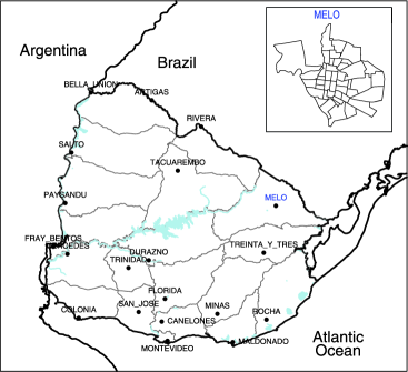
Figure 1: Map of Uruguay with department boundaries and capitals together with the census tracts of Melo.

A total of $p=11$ indicators are observed at the census tract level for all nineteen departmental capitals of Uruguay. These indicators represent the most complete and reliable data set available in Uruguay and were collected during the most recent census in 1996 (Censo Nacional de Población Hogares y Viviendas de 1996).

All the available variables are observed in the census tract level of the $I=19$ Departmental capitals. They have been standardized to represent percentages, averages, densities, etc. Broadly,

Table 1: Description of the $p=11$ variables, observed in the census tract level of the departmental capitals, to build the vulnerability index of the population of Uruguay to vector-borne diseases

Level of vulnerability	Variables
Personal characteristic	Illiteracy rate (ILL)
	Population with access to public health care (PHC)
	Male without formal jobs (UQW)
Household characteristic	Owed houses (OWH)
	Households headed by a woman (WHF)
	Households without sewage system (AHS)
	Average number of persons per household (APH)
	Households with more than two persons per room (OVC)
	Households without access to treated, drinkable water (ADW)
	Households with air conditioner (ACO)
	Households poorly built (HOQ)

the available indicators can be divided into two groups representing general assessments of vulnerability: personal and household conditions. See Table 1 for details.

1.3 Vulnerability via spatial factor models

As vulnerability is related to weighing the influence of many different indicators on a person’s (or group’s) living pattern, it is not surprising that the current literature contains abundant factor and principal component analysis alternatives to build such an index. Factor models and spatial models are, indeed, two successful examples of the broader class of hierarchical models that have been experiencing major attention from the scientific community as well as from practitioners in areas as diverse as climate/environment, economics/finance and health/psychology, among many others. Both areas directly benefited from the accumulated advances in Bayesian computation over the last two decades [see Gamerman and Lopes (2006)]. Fully Bayesian treatments of factor models and spatial models are described, for instance, in Lopes and West (2004) and Banerjee, Carlin and Gelfand (2004), respectively, and their references.

Various versions of spatial factor models have appeared in recent years. For instance, Wang and Wall (2003) and Hogan and Tchernis (2004) model mortality rates and material deprivation measurements, respectively, by first reducing the dimension of the measurement vectors at each spatial location via standard factor analysis, and then spatially modeling the resulting common latent factors. For spatio-temporal problems, Lopes, Salazar and Gamerman (2008), for instance, cluster regions by spatially structuring the factor loadings matrix in a dynamic factor analysis context.

The remainder of the paper is organized as follows. We propose in Section 2 a new class of spatial models, namely, spatial hierarchical factor models (SHFM), that enables the construction of vulnerability indices by combining data observed at all census tracts of some cities of a country, and also avoids loss of information and distortions due to data aggregation. Standard unstructured hierarchical factor models result from our general proposed model and are considered as benchmark models for comparison purposes. Therein, we also discuss a model for observations aggregated at the city level. Our aim is to investigate, for the entertained models, the effect of aggregation when the vulnerability index is used to rank the cities. Section 3 summarizes the steps toward the construction of a micro-environmental index to vector-borne diseases for Uruguay’s capitals and census tracts. As the inference procedure follows the Bayesian paradigm, uncertainty of our estimates are naturally accounted for. Final remarks appear in Section 4.

2 Spatially hierarchical factor model (SHFM)

Let the region under consideration be divided into capitals, each of which is further divided into census tracts. This hierarchy can be expanded down to include more refined layers (levels) depending on the study. For sake of simplicity and without loss of generality, we proceed with two levels: capitals and census tracts. For each one of the $n_{i}$ census tracts of capital $i$, a $p$-dimensional vector of variables (social-economical, environmental, demographical, etc.) is observed, namely, $y_{ij}=(y_{ij1},\ldots,y_{ijp})^{\prime}$, for $i=1,\ldots,I$ and $j=1,\ldots,n_{i}$.

2.1 Observational level

The $p$ region-specific measurements, denoted here by $y_{ij1},\ldots,y_{ijp}$, are used to construct a single factor $f_{ij}$ (the vulnerability factor in our study). More specifically, the observational level of our model is

$$y_{ijk}=\mu_{k}+\beta_{k}f_{ij}+\sigma_{k}\varepsilon_{ijk},\qquad k=1,\ldots,p,$$ (1)

where $\mu_{k}$ represents the overall grand mean vector for measurement $k$. The factor loadings vector $\beta=(1,\beta_{2},\ldots,\beta_{p})^{\prime}$ plays an important role in understanding the role and the composition of the common factor. Its first element is set to one in order to ensure likelihood identifiability [see Lopes and West (2004)]. The specific factors $\varepsilon_{ijk}$ are standard normally distributed and independent across capitals, census tracts and measurements. The impact of the common factor $f_{ij}$ on $y_{ijk}$ can be assessed, as in standard factor analysis, by the proportion of the variance of $y_{ijk}$ explained by $f_{ij}$, that is,

$$\pi_{ijk}=\biggl{(}1+\frac{\sigma_{k}^{2}}{\beta_{k}^{2}\nu_{ij}^{2}}\biggr{)}^{-1},$$ (2)

where $\nu_{ij}^{2}=\mbox{Var}(f_{ij})$. Assume, for illustration, that the variance of the common factor for a given census tract $i$ in a given city $j$ is equal to one. In this case, $\pi_{ijk}=1/(1+\sigma_{k}^{2}/\beta_{k}^{2})$ and the proportion of the variance of the $k$th measurement that is explained by the common factor increases when the component idiosyncratic standard deviation decreases relative to the absolute value of its loading.

2.2 Modeling the factor $f_{ij}$

Within capital $i$, the vector of common factors $f_{i}=(f_{i1},\ldots,f_{in_{i}})^{\prime}$ is decomposed as the sum of two spatially structured components: one that captures the overall mean of the capital, and the other one captures the local structure of the index, in the census tracts’ level, and also accounts for possible effects of neighboring census tracts. More precisely, we assume

$$f_{ij}=\theta_{i}+{\tilde{f}}_{ij}+\sqrt{\omega_{i}}u_{ij},$$ (3)

where $\theta_{i}$ is the common factor for capital $i$, ${\tilde{f}}_{ij}$ is the specific factor for census tract $j$ and capital $i$, and $u_{ij}$ are independent standard normals. The error term $u_{ij}$ accounts for unanticipated, location specific idiosyncrasies. Similar to (2), $\mbox{var}(f_{ij})=\nu_{ij}^{2}=\eta_{i}^{2}+{\tilde{\nu}}_{ij}^{2}+\omega_{i}$, where $\eta_{i}^{2}=\mbox{var}(\theta_{i})$ and ${\tilde{\nu}}_{ij}^{2}=\mbox{var}({\tilde{f}}_{ij})$. Therefore, the unexplained proportion of $\nu_{ij}^{2}$ (due to $u_{ij}$) is given by

$${\tilde{\pi}}_{ij}=\biggl{(}1+\frac{\eta_{i}^{2}+{\tilde{\nu}}_{ij}^{2}}{\omega_{i}}\biggr{)}^{-1}.$$ (4)

Large values of $\omega_{i}$ (relative to $\eta_{i}^{2}$ and ${\tilde{\nu}}_{ij}^{2}$) lead to ${\tilde{\pi}}_{ij}$ close to one and indicates small explanatory power of the common factor $\theta_{i}$ and the specific factor ${\tilde{f}}_{ij}$ for census tract $j$ and capital $i$.

Spatial variation within capitals

As the capitals are divided into census tracts defining irregular subregions, we model the within capital factors ${\tilde{f}}_{i}=({\tilde{f}}_{i1},\ldots,{\tilde{f}}_{in_{i}})^{\prime}$, for $i=1,\ldots,I$, by a proper conditionally autoregressive (CAR) specification [Sun, Tsutakawa and Speckman (1999)]:

$$\tilde{f}_{i}\sim N(0,\tau_{i}^{2}P_{i}),$$ (5)

where $P_{i}=P_{i}(\phi)=(I_{n_{i}}+\phi M_{i})^{-1}$, $M_{i}=D_{i}-W_{i}$, with $w_{ijl}$, the $(j,l)$ component of $W_{i}$, given by $w_{ijl}=1/d_{jl}$ if $j$ and $l$ are neighbors (denoted here by $j\sim l$) and zero otherwise, $d_{jl}=\|s_{j}-s_{l}\|$ is the Euclidean distance between centroids of capitals $j$ and $l$, $D_{i}=\mbox{diag}(w_{i1+},\ldots,w_{in_{i}+})$ and $w_{ij+}=\sum_{l\sim j}w_{ijl}$. The inverse matrix $P_{i}^{-1}$ is diagonally dominant and positive definite [Harville (1997)]. The parameter $\phi$ controls the strength of the association between the components of ${\tilde{f}}_{i}$, with $\phi=0$ implying independence. Equation (5) approaches the intrinsic autoregressive model when $\phi$ approaches infinity [Besag, York and Mollié (1991), Besag and Kooperberg (1995)]. When an intrinsic autoregressive prior distribution is assumed, it is equivalent to imposing a spatial structure on the parameters. We decided for letting the data inform whether the spatial correlation among the census tracts is present. However, it is known that there is little information about $\phi$ above. We actually tried to fit a model using the reference prior suggested by Ferreira and De Oliveira (2007), but convergence was not reached. Therefore, we decided for fixing these parameters at some specific values and used some model comparison to decide which value fits the data best. It is worth pointing out that in the analysis performed in Section 3 we have also fitted a model assuming an intrinsic autoregressive prior for these parameters and the results did not differ much. The variance of $f_{ij}$ from (4) is then given by ${\tilde{\nu}}_{ij}^{2}=\tau^{2}_{i}P_{i,jj}$.

Spatial variation between capitals

We assume that the $\theta_{i}$’s are conditionally independent and Gaussian with common baseline vulnerability factor $\theta_{0}$ and covariance structure driven by the Euclidean distances between the centroids of the capitals, that is,

$$\theta\sim N(1_{I}\theta_{0},\delta^{2}H(\lambda)),$$ (6)

where $\theta=(\theta_{1},\ldots,\theta_{I})$. Although each capital $i$ has its own vulnerability factor, the above model allows borrowing-strength across neighboring regions. The correlation matrix $H$ is fully specified by a Matérn correlation function, that is, $H_{ij}=\rho(\lambda,d_{ij})=2^{1-\lambda_{2}}\Gamma(\lambda_{2})^{-1}(d_{ij}/\lambda_{1})^{\lambda_{2}}\mathcal{K}_{\lambda_{2}}(d_{ij}/\lambda_{1})$, where $\mathcal{K}_{\lambda_{2}}$ is the modified Bessel function of the second kind and of order $\lambda_{2}$, $\lambda=(\lambda_{1},\lambda_{2})$ and $d_{ij}=\|s_{i}-s_{j}\|$ is the Euclidean distance between the centroids $s_{i}$ and $s_{j}$ of capitals $i$ and $j$, for $i,j=1,\ldots,I$. In our application we fixed $\lambda_{2}=1$ since, as suggested by Whittle (1954), this value should play an important role in spatial statistics. It is easy to see that $\eta_{i}^{2}=\mbox{var}(\theta_{i})=\delta^{2}$ for all $i=1,\ldots,I$. Therefore, (4) can be rewritten as

$${\tilde{\pi}}_{ij}=\biggl{(}1+\frac{\delta^{2}+\tau_{i}^{2}P_{i,jj}}{\omega_{i}}\biggr{)}^{-1}.$$ (7)

2.3 Posterior inference and model selection

We now assign the joint prior distribution of the hyperparameters. Here $W\sim N(a,b)$ means that $W$ is normally distributed with mean $a$ and variance $b$, and $Q\sim\operatorname{IG}(c,d)$ means that $Q$ follows an inverse gamma distribution whose probability density function evaluate at $q$ is proportional to $q^{-(c+1)}\exp(-d/q)$.

The joint prior distribution for the remaining parameters is the product of the following independent marginals: $\mu=(\mu_{1},\ldots,\mu_{p})^{\prime}\sim N(\mu_{0},C_{\mu})$, $\beta_{k}\sim N(\beta_{0},C_{0})$, for $k=2,\ldots,p$, $\sigma_{j}^{2}\sim\operatorname{IG}(a_{j},b_{j})$ for $j=1,\ldots,p$, $\omega_{i}\sim\operatorname{IG}(g_{i},h_{i})$, $\tau^{2}_{i}\sim\operatorname{IG}(c_{i},d_{i})$, for $i=1,\ldots,I$, $\theta_{0}\sim N(t_{0},V_{0})$, $p(\delta^{2})\propto 1/\delta^{2}$ and $\lambda_{1}\sim\operatorname{IG}(2,h)$, where $h=d_{\max}/(-2\log(0.05))$ and $d_{\max}$ is the maximum distance between locations [see Schmidt and Gelfand (2003), Banerjee, Carlin and Gelfand (2004) for more details]. Let $\Theta$ be the parameter vector comprising all the unknowns in the model. The posterior distribution of $\Theta$ is proportional to

$$p(\Theta|y) \propto \prod_{i=1}^{I}\Biggl{\{}\prod_{j=1}^{n_{i}}p(y_{ij}|\mu,\beta,f_{ij},\Sigma)\Biggr{\}}p(f_{i}|\theta_{i},{\tilde{f}}_{i},\omega_{i})p({\tilde{f}}_{i}|\tau_{i}^{2},\phi_{i})p(\omega_{i})p(\tau^{2}_{i})$$

$${}\times\Biggl{\{}\prod_{k=2}^{p}p(\beta_{k})p(\sigma_{k}^{2})\Biggr{\}}p(\mu)p(\sigma_{1}^{2})p(\theta|\theta_{0},\delta^{2},\lambda_{1})p(\theta_{0})p(\delta^{2})p(\lambda_{1}).$$

Closed form posterior inference is infeasible and inference for model parameters is facilitated by a customized Markov chain Monte Carlo (MCMC) scheme that combines Gibbs and Metropolis–Hastings steps. Further details about prior selection and posterior inference for our SHFM appear in the supplementary material of Lopes et al. (2011).

Model comparison is based on the deviance information criterion of Spiegelhalter et al. (2002), the expected posterior deviation of Gelfand and Ghosh (1998), and the scoring rules of Gneiting, Balabdaoui and Raftery (2007). We also compute mean square and mean absolute errors. Further details about these model selection criteria appear in the supplementary material of Lopes et al. (2011).

2.4 Vulnerability index at unobserved cities

It is worth noting that $\theta$ can contain (potentially several) unmeasured cities. More specifically, if $\theta\,{=}\,(\theta_{g}^{\prime},\allowbreak\theta_{u}^{\prime})^{\prime}$ with $\theta_{u}$ the vector of vulnerability for unmeasured cities, then, from (6), it can be shown that $(\theta_{u}|\theta_{g})$ is also normally distributed (conditionally on the hyperparameters) and posterior inference is directly available. More specifically, if $H_{gg}$, $H_{ug}$ and $H_{uu}$ define the corresponding partition of $H$, then the prior mean and prior variance of $(\theta_{u}|\theta_{g})$ are $1_{I}\theta_{0}+H_{ug}H_{gg}^{-1}(\theta_{g}-1_{I}\theta_{0})$ and $\delta^{2}(H_{uu}-H_{ug}H_{gg}^{-1}H_{gu})$, respectively. See Section 3 for more details and Figure 2 for posterior inference for $\theta_{g}$ or $\theta_{u}$ for the Uruguayan study.

2.5 Related factor models

Unstructured model

We also fit an unstructured hierarchical factor model (UHFM) to the Uruguayan data. The UHFM is a particular case of our SHFM without accounting for the spatial dependence. This is done by setting $\tilde{f}_{i}=0$, $i=1,\ldots,I$, in (3), and assuming $H(\lambda)=I_{I}$. More specifically,

$$y_{ij} = \mu+\beta f_{ij}+\varepsilon_{ij},$$

$$f_{i} = 1_{n_{i}}\theta_{i}+\sqrt{\omega_{i}}u_{i},$$

$$\theta \sim N(1_{I}\theta_{0},\delta^{2}I_{I})$$

for $\mu$, $f_{i}$, $\omega_{i}$ ($i=1,\ldots,I)$, $\theta_{0}$ and $\delta^{2}$ as previously defined. Further details about posterior inference for this UHFM appear in the supplementary material of Lopes et al. (2011). In Section 3 we compare our SHFM to the UHFM.

Models for aggregated data

As information for all census tracts of Uruguay is unavailable, a standard way to proceed would be to build an index based on the observed mean (across census tracts) of each of the variables at the city level. More specifically, for capitals $i=1,\ldots,I$, let $\overline{y}_{i}=(\overline{y}_{i1},\ldots,\overline{y}_{ip})$ be a $p$-dimensional vector of characteristics such that $\overline{y}_{ik}=n_{i}^{-1}\sum_{j=1}^{n_{i}}y_{ijk}$ $(k=1,\ldots,p)$. In Section 3 we compare our SHFM to when the data are aggregated. For this, we propose an aggregated spatial factor model (ASFM) for which we assume

$$\overline{y}_{i} \sim N(\mu+\beta f_{i},\Sigma),$$

$$f \sim N(1_{I}\theta_{0},\delta^{2}H(\lambda))$$

for $\mu$, $\beta$, $\Sigma$, $\theta_{0}$, $\delta$ and $H(\lambda)$ as previously defined, and here $f=(f_{1},\ldots,f_{I})^{\prime}$.

Assuming a vector of observations $\overline{y}=(\overline{y}_{1},\ldots,\overline{y}_{I})$, the likelihood function is given by

$$f(\overline{y}\mid\mu,\beta,f,\Sigma)=\prod_{i=1}^{I}p(\overline{y}_{i}|\mu,\beta,f_{i},\Sigma),$$ (9)

which is based only on the observations at the $I$ cities. Unlike our HSFM, the ASFM’s vulnerability index is given by the component $f_{i}$. We also consider the simpler case where the components of $f$ are spatially independent, that is, a simple aggregated factor model (AFM) for which the matrix $H(\lambda)$ is an identity matrix of dimension $I$. A major drawback of these aggregated models is that they do not take into account the fact that the cities have a different number of census tracts.

Spatial factor models

Our hierarchical spatial factor model is closely related to Wang and Wall (2003) and Hogan and Tchernis (2004) spatial factor models. For instance, Hogan and Tchernis’s spatial factor models are used to construct one-dimensional model-based deprivation indexes for Rhode Island’s census tracts. Their models are special cases of our SHFM via equations (1) and (5). More specifically, they consider $I=1$ (Rhode Island) and $n_{1}=228$ for (1) and a variety of spatial structures for $P$ in (5).

3 Building an Uruguayan vulnerability index

The models discussed in Section 2 are used to construct the vulnerability index for the Uruguayan data described in Section 1. In particular, we investigate the effect of aggregating the data across the city. The MCMC algorithm was run for a total of 30,000 iterations with 10,000 burn-in iterations. For each model, we ran two parallel chains starting at different initial points of the parametric space. Posterior inference was based on the last 20,000 iterations, recording every 5th iteration in order to avoid possible autocorrelations. We check the convergence of all chains via Brooks and Gelman’s (1998) modification of the Gelman–Rubin statistic.

Table 2 presents model comparison results based on the criteria described in the supplementary material of Lopes et al. (2011). We fit the UHFM with $\theta=0$ and with unknown $\theta$. We fit the SHFM with $\phi=1$, $5$ and $7$, where the greater the value of $\phi$, the stronger the spatial correlation between the components of $\tilde{f}_{i}$. Our SHFM, with $\phi=5$ or $\phi=7$, is chosen as the best model by all five criteria. In addition, we have performed residual analysis to investigate the goodness of fit of the proposed model. We checked whether the standardized residuals follow a standard normal distribution. Q–Q plots of the residuals (not shown) for the best fitted spatial hierarchical factor model indicate that the quantiles from the model are consistent with the normal quantile. In addition, Table 2 shows MSE and MAE measurements that provide further information about goodness of fit. Hence, the following results are based on the SHFM with $\phi=5$.

Table 2: Comparing SHFM and UHFM: comparing the unstructured hierarchical factor (UHFM) and spatial hierarchical factor models (SHFM) for different values of $\phi$. Best models appear in italic. DIC: deviance information criterion, EPD: expected posterior deviation, CRPS: continuous ranked probability score, MSE: mean square error and MAE: mean absolute error. CRPS are in tens of thousands

	UHFM		SHFM
Criterion	$\bolds{\theta=0}$	Unknown $\bolds{\theta}$	$\bolds{\phi=1}$	$\bolds{\phi=5}$	$\bolds{\phi=7}$
DIC	$-$21,445.4	$-21\mbox{,}493.3$	$-$21,785.8	$-$21,827.4	$-$21,827.0
EPD	2,557.4	$2\mbox{,}510.9$	2,453.1	2,433.6	2,432.6
CRPS	1,030.7	$1\mbox{,}024.2$	1,014.2	1,010.3	1,010.3
MAE	2,397.0	$2\mbox{,}381.8$	2,374.5	2,367.9	2,369.1
MSE	1,222.3	$1\mbox{,}200.1$	1,177.2	1,169.2	1,168.9

Table 3 (columns 2–9) presents the percentage of the variability of each variable (averaged across census tracts) that is explained by the vulnerability index [see (2)]. The rows are ordered from the largest to the smallest percentage of the variance, starting with the first column (ILL), then moving to the second column (PHC) for ties, and so on.

Table 3: Variance decomposition. Columns 2–9: percentage of the variance explained by the vulnerability index under model SHFM ($\phi=5$) and averaged across census tracts within a given capital. Percentages are below 10 for OWH, WHF and ACO. The rightmost column (VAR) is the percentage of the variance explained by the common factor $\theta_{i}+\tilde{f}_{ij}$ averaged across census tracts [equation (4)]

Capital	ILL	PHC	OVC	UQW	AHS	ADW	APH	HOQ	VAR
Bella Unión	95	93	90	79	77	70	58	51	77
Rivera	92	90	86	72	69	61	48	41	93
Treinta y Tres	92	90	86	72	69	61	48	41	87
Melo	92	90	85	70	67	59	46	39	93
Salto	91	89	84	69	66	57	45	38	92
Tacuarembó	91	89	84	69	65	57	44	37	90
Canelones	91	89	84	68	65	57	44	37	77
Fray Bentos	91	89	84	68	65	57	44	37	90
Mercedes	91	89	84	68	65	56	44	37	91
Durazno	91	88	83	68	65	56	43	37	90
Colonia	91	88	83	68	64	56	43	36	91
Rocha	91	88	83	68	64	56	43	36	91
Paysandú	91	88	83	67	64	55	43	36	95
Trinidad	90	88	83	67	64	55	42	36	85
Florida	90	88	83	67	63	55	42	35	90
San José	90	88	82	66	63	54	41	35	90
Maldonado	90	87	82	65	62	53	41	34	93
Minas	89	87	81	64	61	52	39	33	90
Montevideo	77	73	64	42	39	31	21	17	97
Uruguay	90	88	83	67	64	56	43	36	90

The index impact is higher on ILL, PHC and OVC, each one representing a different socioeconomic characteristic: education, health care and household structure, respectively. These results reveal a strong connection between the index and education and health. Apart from Montevideo, the pattern is relatively similar across the country, as indicated by the bottom row of the table. It is interesting to note that the order of the capitals also obey a North to South decrease in the impact of the index with a slight northwest–southeast rotation. This North–South behavior is clear in the results that follow. In addition, the rightmost column of Table 3 presents the percentages of the variances explained by the common factor $\theta_{i}+\tilde{f}_{ij}$ averaged across census tracts [see (4)]. For most of the capitals, the explained variability is around 90%, indicating the explanatory power of these two measurements.

Figure 2 shows the posterior mean and posterior standard deviations of the component $\theta_{i}$ of the vulnerability index for measured and unmeasured cities in Uruguay under the SHFM with $\phi=5$. We have standardized the values of $\theta$, and the lower its value, the better the index. The index in the country level presents a clear spatial pattern. It assumes low values in the South of the country and increases smoothly toward the North–Northwest region of Uruguay. This is in accordance with the consolidation of urban structures, showing that $\theta$ is capturing the conditions of the micro-environment of the population. Although Montevideo concentrates most of the population of the country, we notice that the index indicates its surrounds as being the least vulnerable. On the other hand, the North of the country results in the highest values of $\theta$, corresponding to the poor conditions of these cities and their suburbs. Also, these are regions that share a border with Argentina and Brazil, and the migration within this region is much greater than the improvement that has been made on basic services for the population. Again, this component is clearly capturing this characteristic. Standard errors vary across the region, such that the closer to monitored locations the lower their values, and are at most one fifth of the corresponding index.

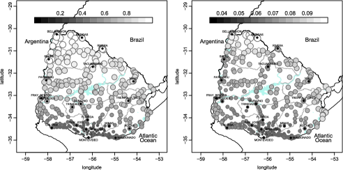
Figure 2: Posterior mean of $\theta_{i}$ and standard deviations (second column) for observed and unobserved cities under the SHFM when $\phi=5$.

Figure 3 depicts the effect of either assuming (i) a spatially structured prior distribution or (ii) an independent prior for $\theta$, as well as the effect of modeling either (i) the disaggregated data or (ii) the aggregated data. It is clear that the range of the posterior distribution of $\theta$ under SHFM is shorter than that obtained under the assumption that the $\theta$’s are independent a priori (model UHFM). Concentrating on the results when we fit the model for the aggregated data, the spatial model (ASFM) also results in shorter ranges of the posterior distribution of $\theta$. However, when comparing SHFM to ASFM, the ranges of the posterior distribution of $\theta_{i}$ under aggregated data (ASFM) do not differ across capitals.

Figure 3: Posterior means of the $\theta_{i}$ (black dots) and 95% CI (vertical lines) for each of the 19 capitals under the different models. Top row: SHFM with $\phi=5$ (left) and UHFM (right). Bottom row: ASFM (left) and AFM (right). The quantities on the top of the top row boxes are the number of census tracts for each capital.

This is expected as the model under the aggregated data does not consider the information about the number of census tracts in each capital. This suggests that the spatial model for the aggregated data provides conservative estimates of the underlying uncertainty when estimating $\theta$. Additionally, by ranking the cities based on the vulnerability index posterior mean, it can be seen that Canelones and San José are at positions 5 and 7, despite their proximity to Montevideo (under UHFM, ASFM and AFM). Our SHFM corrects this distortion and ranks these capitals in positions 2 and 3.

Figure 4: Posterior rankings of the capitals. Top row: SHFM with $\phi=5$ (left) and UHFM (right). Bottom row: ASFM (left) and AFM (right). The quantities at the top of each box are the number of census tracts for each capital.

An important contribution of our modeling strategy is the possibility of probabilistically ranking the vulnerability across capitals. Figure 4 compares posterior vulnerability rankings based on our SHFM with $\phi=5$ and the benchmark models, that is, the UHFM, the ASFM and the AFM. Our SHFM captures the South-to-North spatial vulnerability increase in Uruguay, as anticipated by the experts. On the one hand, Montevideo and Canelones are the least vulnerable capitals, followed closely by San José, Colonia, Minas and Maldonado, all of them located in the South region of the country and all of them somewhat near Montevideo. On the other hand, Bella Unión, Salto, Rivera, Tacuarembó, Melo and Paysandú are the most vulnerable capitals, all of them located in the north and northwest regions of the country. These findings corroborate with our previous findings (see Figure 2). The UHFM is the model with the closest ranking pattern, at the capital level, when compared to our SHFM. However, it suffers from its lack of spatial structure, which leads to different ranking of the cities, in particular, Canelones, Colonia and Minas. More critically, the UHFM underestimates the uncertainty associated with the rankings. Not surprisingly, such behavior is even more marked under the ASFM and the AFM, where any local structure is distorted or eliminated by the aggregation of the data. See, for example, the discussions in Schmidtlein et al. (2008).

As we propose a factor model for data observed in the census tract level, following our SHFM, we are able to investigate the components of the index at each census tract of each city in the sample. Panels of Figure 5 show the posterior mean of a standardized version of $f_{ij}$

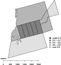
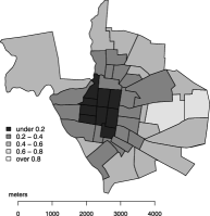
(a)	(b)
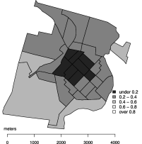
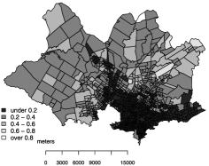
(c)	(d)

Figure 5: Within-city posterior vulnerability index per census tract of (a) Bella Unión, (b) Melo, (c) Florida and (d) Montevideo. Values were standardized to allow for comparison among the cities. Each map shows $\kappa_{ij}=(f_{ij}-{\underline{f}})/({\overline{f}}-{\underline{f}})$, where ${\overline{f}}=\max_{i,j}f_{ij}$ and ${\underline{f}}=\min_{i,j}f_{ij}$.

(again under SHFM with $\phi=5$) for each census tract from Bella Unión, Melo, Florida and Montevideo. Standardization was an artifact to make the country level effects visually comparable. More precisely, the standardized within-city posterior vulnerability index is given by $\kappa_{ij}=(f_{ij}-{\underline{f}})/({\overline{f}}-{\underline{f}})$, where ${\overline{f}}=\max_{i,j}f_{ij}$ and ${\underline{f}}=\min_{i,j}f_{ij}$. These maps provide evidence of the potentiality of our model in decomposing the index as the sum of global and local effects.

In panel (a) we have the posterior mean of $\kappa_{ij}$ for the $11$ census tracts of Bella Unión. The city has lower vulnerability in its center, where more infrastructure and more favorable environmental conditions can be found. An interesting point is that the model is able to differentiate the two census tracts with more controversial environmental conditions in the city. In panel (b) we have the posterior mean of $\kappa_{ij}$ for the $43$ census tracts of Melo which share the border with Brazil. The main activity of this conservative region is cattle raising, and this is concentrated on a small percentage of its population. For this reason, this is a region with high levels of informal activities and lack of basic public services, specially in its outskirts. This is what the estimates of $\kappa_{ij}$ indicate; the central region has values comparable to the good conditions that can be found in the South of the country. Panel (c), on the other hand, shows the posterior mean of the local effects for the $31$ census tracts of Florida, the main city in the area of dairy production in the country. During the twentieth century, Florida had a good socioeconomic status. Also its location, in the half plain of Santa Lucia Chico’s river, allowed it to achieve high standards in environmental terms. With the applications of neo-liberal policies during the 80s and 90s, small dairy producers lost profitability and left the sector. This resulted in a migration to the periphery of the city, which happened much faster than the development of the necessary urban infrastructure. This is clearly represented by the “concentric rings” in panel (c). That is, Florida has good micro-environmental conditions at the developed city center, and the levels of these conditions decrease with the increase of the distance to its center.

Montevideo, the capital of the country, appears in panel (d) with its $1\mbox{,}031$ census tracts. The distribution of $\kappa_{ij}$ across the city allows one to discriminate between very opposing situations, varying from very low to high values of the parameter, capturing the local effects of the index. This is clear in the richest area of the city (Southeast) where there are few census tracts with high values of the index, representing high vulnerability. Land in these regions is irregularly owned. Overall, the levels of $\kappa_{ij}$ in Montevideo are in accordance to what is anticipated by experts, showing high values (more vulnerability) toward the North–West region which comprises more rural areas.

4 Discussion

We proposed a spatially structured factor model to build a vulnerability index based on measurements observed at the census tracts level of a country. In our specific case, we had available observations of $p=11$ indicators at each of the census tracts of the $I=19$ Departmental capitals of Uruguay.

A key issue in our data set is that the number of census tracts in Montevideo is much larger than any of the other capitals, and any factor analysis must take this information into account. To this end, our proposed model provides an index at each census tract which is decomposed as the sum of an overall capital effect and a local effect. In our model the number of census tracts in each capital is naturally accounted for, as described in (3). Also, our model allows the overall effect and the local effects of a city to be spatially structured, and independent models are particular cases of the general structure proposed in Section 2. Model comparison can be used to point which model fits the data best. We entertained among 5 different criteria, and all of them agreed that for our data set it is better to use a model with a spatially structured prior for both $\theta_{i}$ and $\tilde{f}_{i}$.

As inference is performed following the Bayesian paradigm, we are able to obtain summaries of the posterior distribution of any function of the parameters. In particular, our model-based approach provides the estimated ranking of the cities according to the estimated index under the different models (SHFM, UHFM, ASFM and AFM). From the panels in Figure 4 it is clear that the aggregation seriously affects the estimation of the ranking of the vulnerability of the cities. This is expected, as the likelihood function does not consider the different number of census tracts among the cities. Moreover, the spatial structure, anticipated by experts, is lost when the index is estimated based on the aggregated data. Our results indicate that in Uruguay this vulnerability index increases from the South to the North of the country, assuming higher values in the regions close to the border with Brazil and Argentina.

When the goal is the estimation of an index, similar to the ones we developed here, one is advised to carefully and meticulously understand and explore the data and its aggregation structure before proposing any inferential and model selection strategies. Specifically, when the data comprise spatially referenced observations, it is important to explore models which allow for spatial dependence. It is also critically important to acknowledge that aggregating observations might lead to different, perhaps misleading, results.

The resultant index is a valuable management tool in public health. For a country with limited funds such as Uruguay, setting funds allocation priorities based on solid scientific criteria can be a major challenge. Our study aimed at providing such a tool. The next step is to validate our estimated index. This is usually done by performing a qualitative assessment of the index. For example, O’Brien et al. (2004) performed local case studies by visiting highly vulnerable and less vulnerable districts. They interviewed government officials and also nongovernmental organizations; household surveys were also carried out. This is the next step of our research project.

References

- Adger (2006) {barticle}[author] \bauthor\bsnmAdger, \bfnmW. Neil\binitsW. N. (\byear2006). \btitleVulnerability. \bjournalGlobal Environmental Change \bvolume16 \bpages268–281. \bptokimsref \endbibitem
- Banerjee, Carlin and Gelfand (2004) {bbook}[author] \bauthor\bsnmBanerjee, \bfnmS.\binitsS., \bauthor\bsnmCarlin, \bfnmB. P.\binitsB. P. and \bauthor\bsnmGelfand, \bfnmA. E.\binitsA. E. (\byear2004). \btitleHierarchical Modeling and Analysis for Spatial Data. \bpublisherChapman and Hall/CRC, \baddressLondon. \bptokimsref \endbibitem
- Beltrami (2008) {bmisc}[author] \bauthor\bsnmBeltrami, \bfnmM.\binitsM. (\byear2008). \bhowpublishedEvolución de la pobreza em Uruguay por el método del ingreso. Período 1986–2001 (in Spanish). Technical report, Instituto Nacional de Estadística, República Oriental del Uruguay. \bptokimsref \endbibitem
- Besag and Kooperberg (1995) {barticle}[mr] \bauthor\bsnmBesag, \bfnmJulian\binitsJ. and \bauthor\bsnmKooperberg, \bfnmCharles\binitsC. (\byear1995). \btitleOn conditional and intrinsic autoregressions. \bjournalBiometrika \bvolume82 \bpages733–746. \bidissn=0006-3444, mr=1380811 \bptokimsref \endbibitem
- Besag, York and Mollié (1991) {barticle}[mr] \bauthor\bsnmBesag, \bfnmJulian\binitsJ., \bauthor\bsnmYork, \bfnmJeremy\binitsJ. and \bauthor\bsnmMollié, \bfnmAnnie\binitsA. (\byear1991). \btitleBayesian image restoration, with two applications in spatial statistics (with discussion). \bjournalAnn. Inst. Statist. Math. \bvolume43 \bpages1–59. \biddoi=10.1007/BF00116466, issn=0020-3157, mr=1105822 \bptnotecheck related\bptokimsref \endbibitem
- Blaikie et al. (1994) {bbook}[author] \bauthor\bsnmBlaikie, \bfnmP.\binitsP., \bauthor\bsnmCannon, \bfnmT.\binitsT., \bauthor\bsnmDavis, \bfnmI.\binitsI. and \bauthor\bsnmWisner, \bfnmB.\binitsB. (\byear1994). \btitleAt Risk, Natural Hazards, People’s Vulnerability and Disasters. \bpublisherRoutledge, \baddressLondon. \bptokimsref \endbibitem
- Brooks and Gelman (1998) {barticle}[mr] \bauthor\bsnmBrooks, \bfnmStephen P.\binitsS. P. and \bauthor\bsnmGelman, \bfnmAndrew\binitsA. (\byear1998). \btitleGeneral methods for monitoring convergence of iterative simulations. \bjournalJ. Comput. Graph. Statist. \bvolume7 \bpages434–455. \biddoi=10.2307/1390675, issn=1061-8600, mr=1665662 \bptokimsref \endbibitem
- Clark et al. (2000) {bmisc}[author] \bauthor\bsnmClark, \bfnmW. C.\binitsW. C. \betalet al. (\byear2000). \bhowpublishedAssessing vulnerability to global environmental risks. Technical Report 2000-12, Belfer Center for Science and International Affairs, John F. Kennedy School of Government, Harvard Univ. \bptokimsref \endbibitem
- Cutter, Boruff and Shirley (2003) {barticle}[author] \bauthor\bsnmCutter, \bfnmS. L.\binitsS. L., \bauthor\bsnmBoruff, \bfnmB. J.\binitsB. J. and \bauthor\bsnmShirley, \bfnmW. L.\binitsW. L. (\byear2003). \btitleSocial vulnerability to environmental hazards. \bjournalSocial Science Quarterly \bvolume84 \bpages242–261. \bptokimsref \endbibitem
- Eakin and Luers (2006) {barticle}[author] \bauthor\bsnmEakin, \bfnmH.\binitsH. and \bauthor\bsnmLuers, \bfnmA. L.\binitsA. L. (\byear2006). \btitleAssessing the vulnerability of social–environmental systems. \bjournalAnnu. Rev. Environ. Resour. \bvolume31 \bpages365–394. \bptokimsref \endbibitem
- Ferreira and De Oliveira (2007) {barticle}[mr] \bauthor\bsnmFerreira, \bfnmMarco A. R.\binitsM. A. R. and \bauthor\bsnmDe Oliveira, \bfnmVictor\binitsV. (\byear2007). \btitleBayesian reference analysis for Gaussian Markov random fields. \bjournalJ. Multivariate Anal. \bvolume98 \bpages789–812. \biddoi=10.1016/j.jmva.2006.07.005, issn=0047-259X, mr=2322129 \bptokimsref \endbibitem
- Gamerman and Lopes (2006) {bbook}[mr] \bauthor\bsnmGamerman, \bfnmDani\binitsD. and \bauthor\bsnmLopes, \bfnmHedibert Freitas\binitsH. F. (\byear2006). \btitleMarkov Chain Monte Carlo: Stochastic Simulation for Bayesian Inference, \bedition2nd ed. \bpublisherChapman and Hall/CRC, \baddressBoca Raton, FL. \bidmr=2260716 \bptokimsref \endbibitem
- Gelfand and Ghosh (1998) {barticle}[mr] \bauthor\bsnmGelfand, \bfnmAlan E.\binitsA. E. and \bauthor\bsnmGhosh, \bfnmSujit K.\binitsS. K. (\byear1998). \btitleModel choice: A minimum posterior predictive loss approach. \bjournalBiometrika \bvolume85 \bpages1–11. \biddoi=10.1093/biomet/85.1.1, issn=0006-3444, mr=1627258 \bptokimsref \endbibitem
- Gneiting, Balabdaoui and Raftery (2007) {barticle}[mr] \bauthor\bsnmGneiting, \bfnmTilmann\binitsT., \bauthor\bsnmBalabdaoui, \bfnmFadoua\binitsF. and \bauthor\bsnmRaftery, \bfnmAdrian E.\binitsA. E. (\byear2007). \btitleProbabilistic forecasts, calibration and sharpness. \bjournalJ. R. Stat. Soc. Ser. B Stat. Methodol. \bvolume69 \bpages243–268. \biddoi=10.1111/j.1467-9868.2007.00587.x, issn=1369-7412, mr=2325275 \bptokimsref \endbibitem
- Hahn, Riederer and Foster (2009) {barticle}[author] \bauthor\bsnmHahn, \bfnmM.\binitsM., \bauthor\bsnmRiederer, \bfnmA.\binitsA. and \bauthor\bsnmFoster, \bfnmS.\binitsS. (\byear2009). \btitleThe livelihood vulnerability index: A pragmatic approach to assessing risks from climate variability and change—a case study in Mozambique. \bjournalGlobal Environmental Change \bvolume19 \bpages74–88. \bptokimsref \endbibitem
- Harville (1997) {bbook}[author] \bauthor\bsnmHarville, \bfnmD. A.\binitsD. A. (\byear1997). \btitleMatrix Algebra from a Statistician’s Perspective. \bpublisherSpringer, \baddressNew York. \bptokimsref \endbibitem
- Hogan and Tchernis (2004) {barticle}[mr] \bauthor\bsnmHogan, \bfnmJoseph W.\binitsJ. W. and \bauthor\bsnmTchernis, \bfnmRusty\binitsR. (\byear2004). \btitleBayesian factor analysis for spatially correlated data, with application to summarizing area-level material deprivation from census data. \bjournalJ. Amer. Statist. Assoc. \bvolume99 \bpages314–324. \biddoi=10.1198/016214504000000296, issn=0162-1459, mr=2109313 \bptokimsref \endbibitem
- Lopes, Salazar and Gamerman (2008) {barticle}[author] \bauthor\bsnmLopes, \bfnmH. F.\binitsH. F., \bauthor\bsnmSalazar, \bfnmE.\binitsE. and \bauthor\bsnmGamerman, \bfnmD.\binitsD. (\byear2008). \btitleSpatial dynamic factor models. \bjournalBayesian Anal. \bvolume3 \bpages759–792. \bptokimsref \endbibitem
- Lopes and West (2004) {barticle}[mr] \bauthor\bsnmLopes, \bfnmHedibert Freitas\binitsH. F. and \bauthor\bsnmWest, \bfnmMike\binitsM. (\byear2004). \btitleBayesian model assessment in factor analysis. \bjournalStatist. Sinica \bvolume14 \bpages41–67. \bidissn=1017-0405, mr=2036762 \bptokimsref \endbibitem
- Lopes et al. (2011) {bmisc}[author] \bauthor\bsnmLopes, \bfnmH. F.\binitsH. F., \bauthor\bsnmSchmidt, \bfnmA. M.\binitsA. M., \bauthor\bsnmSalazar, \bfnmE.\binitsE., \bauthor\bsnmGoméz, \bfnmM.\binitsM. and \bauthor\bsnmAchkar, \bfnmM.\binitsM. (\byear2011). \bhowpublishedSupplement to “Measuring the vulnerability of the Uruguayan population to vector-borne diseases via spatially hierarchical factor models.” DOI:10.1214/11-AOAS497SUPPA, DOI:10.1214/11-AOAS497SUPPB. \bptokimsref \endbibitem
- Lyth, Holbrook and Beggs (2005) {barticle}[author] \bauthor\bsnmLyth, \bfnmA.\binitsA., \bauthor\bsnmHolbrook, \bfnmN.\binitsN. and \bauthor\bsnmBeggs, \bfnmP.\binitsP. (\byear2005). \btitleClimate, urbanization and vulnerability to vector-borne disease in subtropical coastal Australia: Sustainable policy for a changing environment. \bjournalGlobal Environmental Change Part B: Environmental Hazards \bvolume6 \bpages189–200. \bptokimsref \endbibitem
- O’Brien et al. (2004) {barticle}[author] \bauthor\bsnmO’Brien, \bfnmK. L.\binitsK. L., \bauthor\bsnmLeichenko, \bfnmR.\binitsR., \bauthor\bsnmKelkarc, \bfnmU.\binitsU., \bauthor\bsnmVenemad, \bfnmH.\binitsH., \bauthor\bsnmAandahl, \bfnmG.\binitsG., \bauthor\bsnmTompkins, \bfnmH.\binitsH., \bauthor\bsnmJaved, \bfnmA.\binitsA., \bauthor\bsnmBhadwal, \bfnmS.\binitsS., \bauthor\bsnmNygaard, \bfnmS. Barg L.\binitsS. B. L. and \bauthor\bsnmWest, \bfnmJ.\binitsJ. (\byear2004). \btitleMapping vulnerability to multiple stressors: Climate change and globalization in India. \bjournalGlobal Environmental Change \bvolume14 \bpages303–313. \bptokimsref \endbibitem
- Reid et al. (2009) {barticle}[author] \bauthor\bsnmReid, \bfnmC. E.\binitsC. E., \bauthor\bsnmO’Neill, \bfnmM. S.\binitsM. S., \bauthor\bsnmGronlund, \bfnmC. J.\binitsC. J., \bauthor\bsnmBriness, \bfnmS. J.\binitsS. J., \bauthor\bsnmBrown, \bfnmD. G.\binitsD. G., \bauthor\bsnmDiez-Roux, \bfnmA. V.\binitsA. V. and \bauthor\bsnmSchwartz, \bfnmJ.\binitsJ. (\byear2009). \btitleMapping community determinants of heat vulnerability. \bjournalEnvironmental Health Perspectives \bvolume117 \bpages1730–1735. \bptokimsref \endbibitem
- Rue et al. (2007) {bmisc}[author] \bauthor\bsnmRue, \bfnmH.\binitsH., \bauthor\bsnmFollestad, \bfnmT.\binitsT., \bauthor\bsnmWist, \bfnmH. T.\binitsH. T. and \bauthor\bsnmMartino, \bfnmS.\binitsS. (\byear2007). \bhowpublishedGMRFLib: A C-library for fast and exact simulation of Gaussian Markov random fields. Technical report, Dept. Mathematical Sciences, The Norwegian Institute of Technology, Trondheim. \bptokimsref \endbibitem
- Rygel, O’Sullivan and Yarnal (2006) {barticle}[author] \bauthor\bsnmRygel, \bfnmLisa\binitsL., \bauthor\bsnmO’Sullivan, \bfnmDavid\binitsD. and \bauthor\bsnmYarnal, \bfnmBrent\binitsB. (\byear2006). \btitleA method for constructing a social vulnerability index: An application to hurricane storm surges in a developed country. \bjournalMitigation and Adaptation Strategies for Global Change \bvolume11 \bpages741–764. \bptokimsref \endbibitem
- Sarewitz, Pielke and Keykhah (2003) {barticle}[pbm] \bauthor\bsnmSarewitz, \bfnmD.\binitsD., \bauthor\bsnmPielke, \bfnmR.\binitsR. and \bauthor\bsnmKeykhah, \bfnmM.\binitsM. (\byear2003). \btitleVulnerability and risk: Some thoughts from a political and policy perspective. \bjournalRisk Anal. \bvolume23 \bpages805–810. \bidissn=0272-4332, pmid=12926572 \bptokimsref \endbibitem
- Schmidt and Gelfand (2003) {barticle}[author] \bauthor\bsnmSchmidt, \bfnmA. M.\binitsA. M. and \bauthor\bsnmGelfand, \bfnmA. E.\binitsA. E. (\byear2003). \btitleA Bayesian coregionalization model for multivariate pollutant data. \bjournalJournal of Geophysics Research \bvolume108 \bpages8783. \bptokimsref \endbibitem
- Schmidtlein et al. (2008) {barticle}[author] \bauthor\bsnmSchmidtlein, \bfnmMathew C.\binitsM. C., \bauthor\bsnmDeutsh, \bfnmRoland C.\binitsR. C., \bauthor\bsnmPiegorsch, \bfnmWalter W.\binitsW. W. and \bauthor\bsnmCutter, \bfnmSusan L.\binitsS. L. (\byear2008). \btitleA sensitivity analysis of the social vulnerability index. \bjournalRisk Anal. \bvolume28 \bpages1099–1114. \bptokimsref \endbibitem
- Sen (1981) {bbook}[author] \bauthor\bsnmSen, \bfnmA. K.\binitsA. K. (\byear1981). \btitlePoverty and Famines: An Essay on Entitlement and Deprivation. \bpublisherClarendon, \baddressOxford. \bptokimsref \endbibitem
- Spiegelhalter et al. (2002) {barticle}[mr] \bauthor\bsnmSpiegelhalter, \bfnmDavid J.\binitsD. J., \bauthor\bsnmBest, \bfnmNicola G.\binitsN. G., \bauthor\bsnmCarlin, \bfnmBradley P.\binitsB. P. and \bauthor\bparticlevan der \bsnmLinde, \bfnmAngelika\binitsA. (\byear2002). \btitleBayesian measures of model complexity and fit. \bjournalJ. R. Stat. Soc. Ser. B Stat. Methodol. \bvolume64 \bpages583–639. \biddoi=10.1111/1467-9868.00353, issn=1369-7412, mr=1979380 \bptokimsref \endbibitem
- Sun, Tsutakawa and Speckman (1999) {barticle}[mr] \bauthor\bsnmSun, \bfnmDongchu\binitsD., \bauthor\bsnmTsutakawa, \bfnmRobert K.\binitsR. K. and \bauthor\bsnmSpeckman, \bfnmPaul L.\binitsP. L. (\byear1999). \btitlePosterior distribution of hierarchical models using distributions. \bjournalBiometrika \bvolume86 \bpages341–350. \biddoi=10.1093/biomet/86.2.341, issn=0006-3444, mr=1705418 \bptokimsref \endbibitem
- van Leishout et al. (2004) {barticle}[author] \bauthor\bparticlevan \bsnmLeishout, \bfnmM.\binitsM., \bauthor\bsnmKovats, \bfnmR.\binitsR., \bauthor\bsnmLivermore, \bfnmM.\binitsM. and \bauthor\bsnmMartens, \bfnmP.\binitsP. (\byear2004). \btitleClimate change and malaria: Analysis of the SRES climate and socio-economic scenarios. \bjournalGlobal Environmental Change \bvolume14 \bpages87–99. \bptokimsref \endbibitem
- Wang and Wall (2003) {barticle}[pbm] \bauthor\bsnmWang, \bfnmFujun\binitsF. and \bauthor\bsnmWall, \bfnmMelanie M.\binitsM. M. (\byear2003). \btitleGeneralized common spatial factor model. \bjournalBiostatistics \bvolume4 \bpages569–582. \biddoi=10.1093/biostatistics/4.4.569, issn=1465-4644, pii=4/4/569, pmid=14557112 \bptokimsref \endbibitem
- Whittle (1954) {barticle}[mr] \bauthor\bsnmWhittle, \bfnmP.\binitsP. (\byear1954). \btitleOn stationary processes in the plane. \bjournalBiometrika \bvolume41 \bpages434–449. \bidissn=0006-3444, mr=0067450 \bptokimsref \endbibitem