The pulse profile and spin evolution of the accreting pulsar in Terzan 5, IGR J17480-2446, during its 2010 outburst

Abstract

We analyse the spectral and pulse properties of the 11 Hz transient accreting pulsar, IGR J17480-2446, in the globular cluster Terzan 5, considering all the available Rossi X-ray Timing Explorer, Swift and INTEGRAL observations performed during the outburst shown between October and November, 2010.

By measuring the pulse phase evolution we conclude that the NS spun up at an average rate of $<\dot{\nu}>=1.48(2)\times 10^{-12}$ Hz s^-1, compatible with the accretion of the Keplerian angular momentum of matter at the inner disc boundary. This confirms the trend previously observed by Papitto et al. (2011), who considered only the first few weeks of the outburst. Similar to other accreting pulsars, the stability of the pulse phases determined by using the second harmonic component is higher than that of the phases based on the fundamental frequency. Under the assumption that the second harmonic is a good tracer of the neutron star spin frequency, we successfully model its evolution in terms of a luminosity dependent accretion torque. If the NS accretes the specific Keplerian angular momentum of the in-flowing matter, we estimate the inner disc radius to lie between 47 and 93 km when the luminosity attains its peak value. Smaller values are obtained if the interaction between the magnetic field lines and the plasma in the disc is considered.

The phase-averaged spectrum is described by thermal Comptonization of photons with energy of $\approx 1$ keV. A hard to soft state transition is observed during the outburst rise. The Comptonized spectrum evolves from a Comptonizing cloud at an electron temperature of $\approx$ 20 keV towards an optically denser cloud at $kT_{e}\approx$ 3 keV. At the same time, the pulse amplitude decreases from $27\%$ to few per cent, as already noted by Papitto et al. (2011), and becomes strongly energy dependent. We discuss various possibilities to explain such a behaviour, proposing that at large accretion luminosities a significant fraction of the in-falling matter is not channelled towards the magnetic poles, but rather accretes more evenly onto the NS surface.

1 Introduction

The study of the frequency variations of the coherent signal emitted by an accreting pulsar is one of the foremost techniques to study the dynamical interaction between the rotating neutron star (NS in the following) and the in-falling matter. This is particularly the case of disc-fed pulsars since the torque acting on the NS is expected to reflect the specific angular momentum of the disc plasma before it is captured by the pulsar magnetosphere, as well as the interaction between the disc plasma and those magnetic field lines that close through it (see, e.g., Ghosh, 2007, and references therein).

The process of disc angular momentum accretion is also established as the driver to accelerate a NS until it reaches a spin period of few ms. According to the recycling scenario (see, e.g., Bhattacharya & van den Heuvel, 1991) rotation-powered millisecond pulsars are spun up by a long-lasting phase of accretion of mass and of the relative angular momentum by a NS in a low-mass X-ray binary (LMXB). The discovery of coherent ms pulsations in the X-ray emission of a transient LMXB (Wijnands & van der Klis, 1998) provided a fundamental confirmation of this scenario, also opening the possibility of studying the frequency evolution of quickly rotating NS during the accretion phase. However, so far measuring the NS spin evolution while accreting of the known 14 accreting millisecond pulsars (AMSP) has been made often difficult by the intrinsic small torques exerted on the NS of these systems. This is partly due to the relatively short timescales of the accretion episodes, with outbursts lasting generally less than few weeks, and to the relatively small peak outbursts luminosities, which are not observed to exceed a level of few $\times 10^{36}$ erg s^-1. To complicate further the task, timing noise was observed to affect the phase of the pulse profile (see, e.g., Burderi et al., 2006; Hartman et al., 2009). A spin-up at a rate of the order of that expected according to standard accretion theories could then be confirmed only in a couple of cases (Falanga et al., 2005; Burderi et al., 2007; Papitto et al., 2008).

Here we present the case of the 11 Hz accreting pulsar, IGR J17480-2446, belonging to the globular cluster Terzan 5. The temporal evolution of the 11 Hz spin frequency during a subset of all the observations performed by the Rossi X-Ray Timing Explorer (RXTE) and Swift was studied by Papitto et al. (2011, P11 in the following), who found an average spin up rate compatible with accretion of the Keplerian angular momentum of disc matter. The analysis of the Doppler shifts of the signal frequency allowed to measure the 21.27 hr orbital period and to constrain the mass of the companion between 0.4 and 1.5 $M_{\odot}$ (see P11, and the references therein). A candidate IR counterpart was proposed by Testa et al. (2011) thanks to an observation performed by ESO-VLT/NAOS-CONICA while the source was in outburst. This candidate was then identified by Patruno & Milone (2012) in a HST archival observation performed when the source was in quiescence. From the presence of pulsations at the minimum and maximum luminosity P11 estimated the surface magnetic field of the NS to lie between a few times $10^{8}$ and a few times $10^{10}$ G. These properties make this recently detected mildly-recycled pulsar, the only discovered so far in a LMXB to spin at a frequency between 10 and 100 Hz, a unique case study to directly observe the effects of disc torque on the NS through the measure of its spin evolution while accreting. In this paper, we analyse in detail the properties of the energy spectrum (Sec. 3.1) and of the pulse profile (Sec. 3.2) of J17480 using all the available X-ray observations performed by RXTE, Swift, and INTEGRAL, focusing on the effects of the torque exerted on the NS by the disc accreting matter (Sec. 3.3 and 3.4). The results obtained are then discussed in Sec. 4.

2 Observations

In this paper we consider all the observations of IGR J17480-2446 (J17480 in the following) performed by RXTE, Swift and INTEGRAL during the intensive observational campaign which followed the discovery of the source on 2010 October 10.365 (Bordas et al. 2010; MJD 55479.365, all the epochs are given in UTC). The monitoring of the source ended at MJD 55519.130, due to a solar occultation of the sky region where this transient lies. Such obstruction ceased only $\sim$ 2 months later (MJD 55584.562); since further RXTE observations failed to detect an excess above the background it has to be concluded that the J17480 outburst ended during the period of non-visibility.

During the outburst the source showed a large number of X-ray bursts, whose spectral and temporal properties are compatible with thermonuclear burning of a mixed H/He layer on the NS surface (Motta et al., 2011; Chakraborty & Bhattacharyya, 2011; Linares et al., 2011). Since we are here interested in the analysis of the source properties during the non-bursting emission, we discard $\sim$10 s prior the onset of each of the bursts that could be significantly detected above the continuum emission, and a variable interval of length between 50 and 160 s after, depending on the burst decay timescale. During the analysis of observations taken in modes with low temporal resolution (e.g. Standard 2 modes of PCA aboard RXTE) the length of the time intervals excluded from the analysis was increased in order to equal the time-binning.

2.1 RXTE

In this paper we consider data obtained by the Proportional Counter Array (PCA; 2–60 keV Jahoda et al., 2006) during the interval MJD 55482.008–55519.130 (ObsId. 95437). Spectra and response matrices were extracted by using standard tools of the Heasoft software package, version 6.11. The ’bright’ model was used to subtract background emission, and only photons recorded by the top layer of the Proportional Counter Unit (PCU) 2 and falling in the 2.5 – 30 keV energy range were retained in spectral fitting. Further, a systematic error of 0.5% was added to each spectral channel. HEXTE data were not included in the analysis since the background dominates over source photons, and a number of ’line-like’ residuals of calibration origin make the characterisation of the spectral continuum at high energies extremely problematic. In the temporal analysis we retained photons collected by all the PCUs of PCA in the 2–60 keV energy band, and encoded in fast configurations such as Good Xenon and Event, with temporal resolution of 1 and 122 $\mu$s, respectively.

2.2 Swift

The Swift observations of J17480 covered the interval MJD 55479.198–55501.559 (Obs.Ids 31838, 31841, 437313, 437466) and in this paper we consider only data observed by the X-ray Telescope (XRT; 0.2–10 keV; Gehrels et al., 2004). All the data were processed by using standard procedures (Burrows et al., 2005) and the latest calibration files available at the time of the analysis (2011 September; caldb v. 20110725). Spectral analysis was performed on data collected both in window timing (WT) and photon counting (PC) mode (processed with the xrtpipeline v.0.12.6), while only WT data sampled every 1.7 ms, and falling in the 0.2–10 keV, were considered for the temporal analysis. Filtering and screening criteria were applied by using ftools (Heasoft v.6.11). We extracted source and background light curves and spectra by selecting photons in the 1–10 keV energy band and event grades of 0 and 0-12, respectively for the WT and PC mode. Grades 1 and 2 in the WT data were filtered out in order to limit the effect of the recently reported redistribution problem on the source and background product (see the web-page http://www.swift.ac.uk for details). The only observation considered that was performed in PC mode was affected by a strong pile-up, and corrected according to the technique developed by Vaughan et al. (2006). Given the relatively high count-rate of the source during the WT observations, we also checked if these data were affected by pile-up by extracting for each of them a source spectrum from a circular region in which we progressively excluded a larger and larger fraction of the inner central pixels. Fits to these spectra did not reveal any significant change in the model parameters, and thus we assumed that XRT/WT data were not affected by pile-up. Spectral channels were grouped to contain at least 50 counts each, as it was done for all the spectra produced by the various instruments considered in this paper, and a systematic error of 3% was added to each spectral bin.

2.3 INTEGRAL

INTEGRAL observations are commonly divided into “science windows” (SCWs), i.e., pointings with typical durations of $\sim$2-3 ks. We considered all available SCWs that were performed in the direction of the source during the outburst. These comprised publicly available observations of the Galactic bulge (GB) region in satellite revolutions from 975 to 980 (ObsId. 0720001; MJD 55479.365–55491.940), and the data collected during the ToO observation of PKS 1830–211 in rev. 981 (ObsId. 0770005; MJD 55494.778–55497.447). During the GB observations, J17480 was relatively close to the centre of the IBIS/ISGRI telescope (20–150 keV; Lebrun et al., 2003; Ubertini et al., 2003) and thus it was simultaneously observed also with the JEM-X telescope (4.5–25 keV; Lund et al., 2003). During the observations performed in rev. 981, the source was always outside the JEM-X field of view. All INTEGRAL data were analysed using version 9.0 of the OSA software distributed by the ISDC (Courvoisier et al., 2003). JEM-X and ISGRI spectra were rebbinned in order to have 16, 32 or 64 energy channels in the different revolutions, depending on the available statistics of the data.

3 Analysis

3.1 Spectral Analysis.

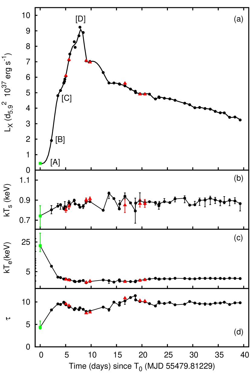
Figure 1: (a) X-ray luminosity of J17480 estimated by extrapolating the best-fitting spectral model, TBAbs*(nthcomp+gaussian), to the 0.05–150 keV energy band. Black points refer to the modelling of the observations performed by PCA on-board RXTE, alone, red triangles to simultaneous XRT-Swift and PCA-RXTE observations, while green squares to simultaneous XRT-Swift, JEMX-INTEGRAL and ISGRI-INTEGRAL observations. The temperature of the soft input photons for Comptonization, the electron temperature of the Comptonizing region, and its optical depth, are plotted in the panels (b), (c) and (d), respectively. Plotted errors are given at the 90% confidence level. The solid line in panel (a) is a cubic spline approximation.

The spectra of the 46 observations performed by PCA were modelled using a thermal Comptonization model (nthcomp, Zdziarski et al., 1996; Życki et al., 1999), with the addition of a Gaussian emission line centred at energies compatible with Iron K-$\alpha$ transition (6.4–6.97 keV). Interstellar absorption was modelled using the TBAbs model (Wilms et al., 2000), fixing the absorption column to the value determined thanks to a 30 ks Chandra observation by Miller et al. (2011), $N_{\mbox{H}}=1.17\times 10^{22}$ cm^-2. The assumed model describes satisfactorily the observed spectra ($\chi^{2}_{r}\simeq 1$; see the rightmost column of Tab. LABEL:tab:xtespectra, where the parameters of the spectral continuum, fluxes in the 2.5–25 keV energy band, and luminosity extrapolated to the 0.05–150 keV band, are also reported for each spectrum).

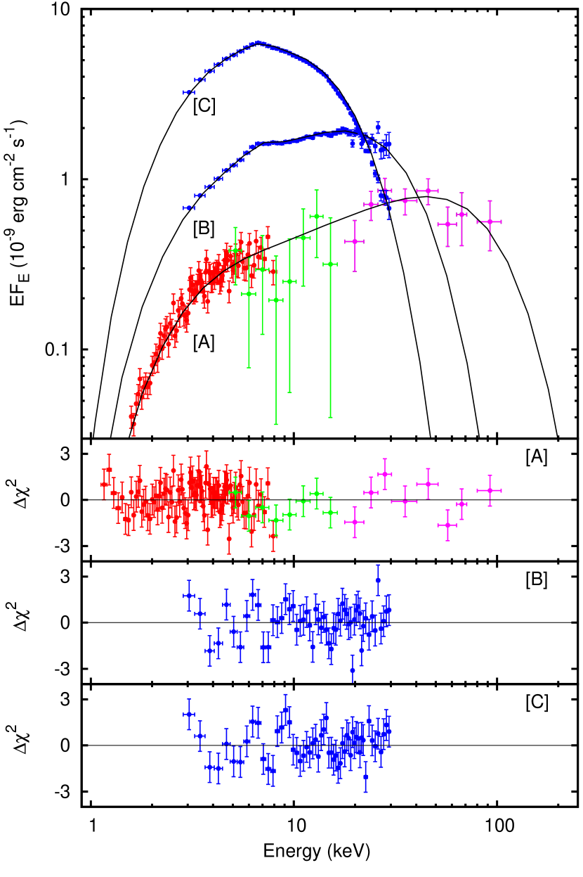
Figure 2: Unfolded spectra accumulated during Swift and INTEGRAL observations covering the intervals 55479.801–55479.824 and 55479.3652–-55479.5483, respectively, [A], and during RXTE observations covering the intervals MJD 55482.008–55482.043 [B] and MJD 55483.715–55483.839 [C], respectively. The best-fitting models, defined as TBAbs*(nthcomp+gaussian), are over-plotted as black solid lines. Points referring to XRT, JEM-X, ISGRI and PCA spectra are plotted as red, green, purple and blue points, respectively. In the lower panels, residuals with respect to the best-fitting models are plotted.

The nthcomp model describes a Comptonized spectrum in terms of the cloud electron temperature , $kT_{e}$, of the temperature of photons injected in the cloud, $kT_{S}$ and of an asymptotic power-law index, $\Gamma$, related to the cloud optical depth, $\tau$, by the relation

$$\Gamma=\left[\frac{9}{4}+\frac{1}{\tau(1+\tau/3)(kT_{e}/m_{e}c^{2})}\right]^{1/2}-\frac{1}{2},$$ (1)

(see, e.g., Lightman & Zdziarski, 1987). The optical depth was then estimated by inverting such a relation, and the relative uncertainty estimated by propagating the statistical errors on $kT_{e}$ and $\Gamma$. The values of the parameters of the Comptonized spectrum measured across the outburst , $kT_{S}$, $kT_{e}$, and $\tau$ are shown as black points in panels (b), (c), and (d) of Fig. 1, respectively. The 3–30 keV spectrum of the source is relatively soft if compared with AMSP (see, e.g., Poutanen, 2006, and references therein). With the exception of the first RXTE observation (labelled as [B] in the top panel of Fig. 1 and spanning the interval MJD 55482.008–5482.043), the electron temperature of the Comptonizing medium is in fact relatively low ($\lower 2.15277pt\hbox{$\;\buildrel<\over{\sim}\;$}3.5$ keV) and the optical depth relatively large ($\tau\approx$ 8–10). By imposing energy conservation between the cold ($kT_{S}\approx 0.9$ keV) and the hot phase ($kT_{e}\approx 3$ keV during most of the observations) producing the Comptonization spectrum, an estimate of the radius of the region that provides the soft photons that are subsequently Comptonized in the hot cloud is obtained. Since the total flux is $F=F_{S}(1+e^{y})$, where $F_{S}=\sigma T_{S}^{4}(R_{S}/d)^{2}$ is the observed flux coming from the colder region and $y=4(kT_{e}/m_{e}c^{2})\tau^{2}$ is the Comptonization parameter, one has $R_{S}=1.8(1/kT_{S})^{2}\sqrt{F/(1+e^{y})}$ d_5.9 km. Here, $kT_{S}$ is expressed in keV and $d_{5.9}$ is the distance to the source in units of 5.9 kpc. By inserting the observed values (see Tab. LABEL:tab:xtespectra) an emitting region with radius between 3 and 15 km is estimated, indicating the NS surface as the most probable region of emission of the soft photons. The iron line detected by PCA appears broad ($\sigma\approx$1 keV) and intense ($\mbox{EW}\approx 0.2$–$0.3$ keV), in accordance with the findings of Miller et al. (2011) and Chakraborty & Bhattacharyya (2011). Its energy is generally compatible with neutral iron (6.4 keV), even if larger values are also sometimes observed.

Figure 3: Error contours on the electron temperature and optical depth measured during observations labeled as [A], [B] and [C] (see text and the caption of Fig. 2), drawn considering the 90% confidence intervals calculated for two parameters ($\Delta\chi^{2}=4.61$).

The accuracy of the spectral modelling obtained from PCA observations was checked by considering the spectra obtained by XRT during the six Swift observations which partly overlapped or were very close in time to RXTE pointings. During all of these observations XRT was operated in WT mode. Spectral fitting was performed by letting the relative normalisation of XRT with respect to PCA free to vary; values in the range 0.92–0.96, with a typical uncertainty of 0.01, were measured. The results obtained are given in Tab. LABEL:tab:swxtespectra. The combined spectra are well described by the model discussed previously, even if residuals are sometimes found at the overlap between the two energy bands. The best-fitting parameters of the simultaneous modelling of XRT and PCA spectra are plotted as red points in Fig. 1, and are visibly very close to the values obtained by modelling PCA spectra alone. The addition of XRT spectra then confirms that the spectral decomposition obtained by analysing PCA data alone is robust. The values of the absorption column obtained with the simultaneous modelling of XRT and PCA spectra are between 1.0 and 1.5$\times 10^{22}$ cm^-2, compatible with the Chandra estimate.

As it was noted earlier, the source emission is soft during the large part of the outburst. Nevertheless, the electron temperature measured during the first PCA observation (labelled as [B] in the top panel Fig. 1), 6.7(2) keV, suggests that a spectral transition from a harder state took place during the outburst rise. To show this spectral change we plot in the top panel of Fig. 2 the unfolded spectra extracted during observations designated as [B] (covering the interval MJD 55482.008–5482.043) and [C] (MJD 55483.715–55483.839; see top panel of Fig. 1). To further investigate this spectral transition, we also considered observations performed by Swift and INTEGRAL before the start of the RXTE coverage on MJD 55482.008 (see label [A] in the top panel of Fig. 1). We then fitted the 1–10 keV Swift XRT spectrum accumulated starting on MJD 55479.801, for an exposure of 2.0 ks (Obs. 00031841002), together with the 4.5–20 keV JEMX-INTEGRAL and the 20–150 keV ISGRI-INTEGRAL spectra accumulated during Rev.975 (spanning MJD 55479.365 – 55479.548, for an exposure of $\sim 8.5$ ks). We normalised the flux observed by JEM-X and ISGRI to that observed by XRT by letting a normalisation constant free to vary. Given the relatively low count rates observed by JEM-X and ISGRI, we held the normalisation constant between these two instruments fixed to 1. No significant improvement in the modelling is obtained otherwise. The spectrum so produced is well fitted by the same Comptonization model used above, with best-fitting parameters, $kT_{S}=0.7(1)$ keV, $kT_{e}=20_{-5}^{+20}$ keV and $\tau=4.4_{-0.4}^{+1.4}$ (see Table LABEL:tab:obsAspectra). These indicate a hotter and optically thinner Comptonizing medium than what is observed during later observations. This is clearly shown in the top panel of Fig. 2, where the unfolded spectrum of the combined XRT, JEM-X and ISGRI spectra is labelled as [A]. The best-fitting parameters of spectrum [A], as well as the luminosity extrapolated to the 0.05-150 keV energy band, are reported in Fig. 1 with green points. To better show the spectral transition performed by J17480 during the outburst rise, and to take into account the correlation between the values of electron temperature and optical depth measured with the Comptonization model we employed (see Eq. 1), we plot in Fig. 3 the 90% confidence level error contours for these parameters. The contours were obtained by considering the surface for which the fit chi-squared was larger by $\Delta\chi^{2}=4.61$ with respect to the best fitting value.

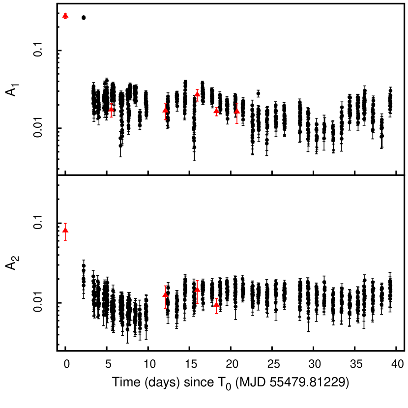
Figure 4: Background-subtracted fractional amplitude of the first (top) and second (bottom) harmonic component used to model the pulse profile of J17480. Red triangles refer to profiles obtained by folding 0.2–10 keV XRT time series around $\nu_{0}=11.044885$ Hz over the entire length of each observation, while black points are obtained by folding 300 s long segments of 2–60 keV PCA data around the same frequency.

A softening of the emission during the outburst rise is also indicated by the analysis of the spectra accumulated by JEM-X and by ISGRI on-board INTEGRAL, alone. We list in Tab. LABEL:tab:igrspectra the results obtained by fitting the spectra accumulated during each of the INTEGRAL revolution with the same model used so far, and keeping the relative normalisation between the two instruments fixed to one. Observations performed before MJD 55483 are well fitted by Comptonization in a medium with $kT_{e}>10$ keV, while subsequent observations indicate temperatures of the order of those indicated by the analysis of XRT and PCA spectra ($\approx 3$ keV). Such a transition is even clearer by taking into account the fluxes observed by JEM-X and ISGRI. Before MJD 55483 the ratio $F_{JEMX}(4.5-25.0)/F_{ISGRI}(20.0-150)$ is $\approx 0.5-1$, while it takes values in excess of 30 during observations performed when the source bolometric luminosity is larger. Moreover ISGRI could not detect the source after MJD 55483, with typical upper limits of $F_{ISGRI}(50-150)<\mbox{few}\>\times\>10^{-11}$–$10^{-12}$ erg cm^-2 s^-1 (3 $\sigma$ confidence level), while the flux in the same energy band is $\approx 5\times 10^{-10}$ erg cm^-2 s^-1 during earlier observations (see the rightmost columns of Tab. LABEL:tab:igrspectra).

Figure 5: Background-subtracted profiles obtained by folding around $\nu_{0}=11.044885$ the 2–60 keV PCA light curves accumulated during observation labelled as [B] (spanning MJD 55482.008–55482.043), [C] (MJD 55483.715–55483.839) and [D] (MJD 55487.565 – 55487.693), when the 0.05–150 keV luminosity was $1.91(4)\times 10^{37}$, $4.81(2)\times 10^{37}$ and $9.23(4)\times 10^{37}$ erg s^-1, respectively. The difference of the phase of the various pulse profiles is interpreted in Sec. 3.3 and 3.4 in terms of the NS spin frequency derivative. Two cycles are plotted for clarity.

Estimates of the bolometric luminosity were obtained by extrapolating the best-fitting models of PCA spectra to the 0.05-150 keV energy band, and using the most updated estimate of the distance to the cluster (d=5.9$\pm$0.5 kpc, Lanzoni et al. 2010). The values we obtained are listed in Tab. LABEL:tab:xtespectra and plotted in panel (a) of Fig. 1. The maximum luminosity, $L_{max}=9.23(4)\times 10^{37}$ d${}_{5.9}^{2}$ erg s^-1, is observed during the observation starting on $\bar{t}=\mbox{MJD}\>55487.63(6)=7.81(6)$ d since $T_{0}$, and labelled as [D] in the top panel of Fig. 1. To give an estimate of the X-ray flux before the start of the RXTE coverage of the outburst, we consider XRT and INTEGRAL observations previously labelled as [A], yielding an estimate $L_{min}=0.44(6)\times 10^{37}$ d${}_{5.9}^{2}$ erg s^-1.

3.2 The pulse profile

To analyse the properties of the pulse profile of J17480 we considered the time-series recorded by PCA in the 2–60 keV energy band and by the XRT in the 0.2–10 keV band. We first applied barycentric corrections on the times of arrival of photons recorded by PCA and XRT, to take into account the motion of the spacecrafts in the Solar System. To this end we considered the position, RA=17^h 48^m 4$\aas@@fstack{s}$831(4), DEC=-24^∘ 46’ 48$\aas@@fstack{\prime\prime}$87(6), determined by Pooley et al. (2010) by comparing a Chandra observation of the source during the outburst with a deeper past Chandra observation of Terzan 5, performed when J17480 was quiescent (Heinke et al., 2006). This postion is compatible with the one derived by Riggio et al. (2012) from a Moon occultation of the transient, observed by RXTE during the first days of the outburst. The NS motion in the binary system was corrected by using the orbital parameters found by P11, who performed a timing analysis on a subset of the observations considered here.

PCA time series were split in 300 s long intervals and folded in 16 phase bins around $\nu_{0}=11.044885$ Hz (see P11). We adopt the criterion given by Leahy (1987) to determine a detection threshold. A signal was detected with a significance larger than 3 $\sigma$ in all PCA observations. Given its lower effective area, the count-rates recorded by XRT are significantly lower and the whole length of each observation was considered in the folding procedure to maximise the counting statistics. A signal could be detected only in 6 out of 18 XRT observations; however, when a detection was missing the upper limit on the signal amplitude was larger than the amplitude indicated by the analysis of quasi-simultaneous PCA observations. The limited signal-to-noise ratio of XRT data sets is then the most plausible reason for these non-detections.

Figure 6: Energy dependence of the RMS amplitude of the pulse profile shown by J17480 during PCA observations performed during the interval MJD 55482.008-55482.043 (labelled as [B]) and MJD 55483.715–55483.839 (labelled as [C]), respectively.

A two-components harmonic decomposition well describes the observed pulse profiles. The evolution of the background-subtracted 2–60 keV fractional amplitude of the first ($A_{1}$) and second harmonic ($A_{2}$) observed by PCA is plotted as black points in the top and bottom panel of Fig. 4, respectively. As it was already noted by Papitto et al. (2011), a sudden variation in the pulse profile properties takes place during the outburst rise. Most noticeably, the fractional amplitude of the first harmonic observed by PCA decreases from values of $\sim 27\%$, measured before MJD 55483, to $\sim 2\%$ during later observations. The second harmonic amplitude is also observed to decrease, though much more smoothly than the amplitude of the fundamental. During the decaying stage of the outburst, the amplitudes of the two harmonic components do not show any other step-like behaviour, following a smooth trend. Even though the different instrumental responses do not allow an immediate comparison, also the amplitude observed by XRT in the 0.2–10 keV energy band follows a similar trend (see red triangles in Fig. 4).

To show the evolution of the pulse profile shape taking place around MJD 55483 we plot in Fig. 5 the background-subtracted profiles observed by PCA during the observation labelled as [B], [C] and [D], covering the intervals MJD 55482.008-55482.043, MJD 55483.715–55483.839 and MJD 55487.565–55487.693, and during which the 0.05-150 keV X-ray luminosity was $1.91(4)\times 10^{37}$, $4.81(2)\times 10^{37}$ and $9.23(4)\times 10^{37}$ erg s^-1, respectively.

Figure 7: Background subtracted pulse profiles in four energy bands accumulated during PCA observations of group [B] (see text). The solid curves are the respective best-fitting harmonic decompositions. Two cycles are plotted for clarity.

Also the energy dependence of the pulse amplitude changes during the outburst rise. To show this, we consider the observations performed by RXTE during the intervals [B] and [C]. Such a choice is made since the pulse properties observed during group [C] data qualitatively represent what is observed during the rest of the outburst. The energy dependence of the (background subtracted) pulse RMS amplitude, $r(E)=[(A_{1}^{2}+A_{2}^{2})/2]^{1/2}$, is plotted in Fig. 6. During observations labelled as [B] the pulse RMS amplitude is roughly constant with an average value of $0.19$. After MJD 55483 instead, the pulses are nearly completely suppressed at low energies and become stronger as the energy increases up to 30 keV (see curve labelled as [C] in Fig. 6). While during observations of group [B] the profile is nearly sinusoidal and shows the same shape in different energy bands, the phase of the two harmonics becomes slightly energy dependent after MJD 55483. To see this, we plot in Fig. 7 and 8 the background subtracted pulse profiles in four PCA energy bands, accumulated during observations labelled as [B] and [C], respectively. During observations of group [B] the profile has a small harmonic content and shows a similar shape in different energy bands. During observations [C] the phase difference between the first and the second harmonic is negligible at low energies, resulting in a nearly symmetric profile shape, whereas, at higher energies, the fundamental lags the second harmonic resulting in a more skewed profile.

Figure 8: Background subtracted pulse profiles in four energy bands accumulated during PCA observations of group [C] (see text). The solid curves are the respective best-fitting harmonic decompositions. Two cycles are plotted for clarity.

3.3 Timing analysis.

The spin evolution of the source during the outburst was investigated under the assumption that the evolution of the phase of the pulse profile is a good proxy of the NS spin, that is

$$\phi(t)-\phi_{0}=-\int_{T_{0}}^{t}[\nu(t^{\prime})-\nu_{f}]dt^{\prime},$$ (2)

where $\nu(t)$ is the spin frequency of the NS, $\nu_{f}$ is the frequency around which the time series are folded and $T_{0}$ = MJD 55479.81229 is the reference epoch of the timing solution. The phases calculated over the first and the second harmonic component are plotted in the top panels of Fig. 9 and 10, respectively. Phases computed over the profiles observed by XRT in the 0.2–10 keV do not show a signficant scatter with respect to PCA phases (2–60 keV). This can be seen from the bottom panels of Fig. 9 and 10, where we plotted the residuals of XRT (red triangles) and PCA (black points) phases with respect to the best-fitting models defined below. We conclude that the influence on the observed phases of the different energy band and response of the two instruments is small, and consider both the values measured by XRT and PCA. Considering PCA phases alone would not significantly alter the results obtained.

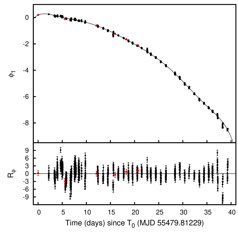
Figure 9: Phases computed over the first harmonic component by folding PCA (2–60 keV; black points) and XRT (0.2–10 keV; red triangles) time series around $\nu_{0}=11.044885$ Hz, together with the best fitting 8-th order polynomial (see text) plotted as a solid line (top panel). Residuals in units of sigma with respect to the best fitting model are plotted in the bottom panel.

To characterise phenomenologically their evolution we fit them with the relation

$$\phi(t)-\phi_{0}=P_{N}(t-T_{0})+R_{orb}(t-T_{0}).$$ (3)

Here, $P_{N}(t-T_{0})=\sum_{n=0}^{N}c_{n}p_{n}(t-T_{0})$ is a $N$-th order polynomial expansion, and the $p_{n}$’s are discrete orthogonal polynomials over the considered data set. Such a choice makes the various fitted parameters, $c_{n}$, independent on the degree of the fitted polynomial, $N$ (see, e.g., Bevington & Robinson, 2003). Defining $x_{i}=t_{i}-T_{0}$, the terms of the polynomial expansion are obtained through the recurrence relation, $p_{n+1}(x)\equiv(x-A_{n+1})p_{n}(x)-B_{n}p_{n-1}(x)$, with $p_{0}(x)=1$ and $p_{-1}(x)=0$. The set of constants $(A_{n},B_{n})$ is determined by imposing orthogonality between the various terms of the polynomial expansion, i.e. $\sum_{i}(1/\sigma_{i}^{2})p_{k}(x_{i})p_{j}(x_{i})=0$, for $k\neq j$, $k,j=0,...,N$. The weights $1/\sigma_{i}^{2}$ simply reflect the uncertainties on the various phase points. The term $R_{orb}(t)$ is added to Eq. 3 to take into account the effect on the phases of a small difference between the orbital parameters used to correct the time series (the orbital period $P_{orb}$, the projected semi-major axis $a\,\sin{i}$ and the epoch of zero mean longitude $T^{*}$) and the actual orbital parameters of the system. An expression for $R_{orb}(t)$ is given by Deeter et al. (1981).

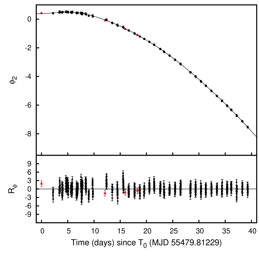
Figure 10: Same as Fig. 9 regarding the phases computed over the second harmonic component.

Small corrections to the orbital parameters are found, leading to the estimates given in Table. 1 (obtained considering a fit with $N=8$, see below). The relatively large values the $\chi^{2}_{r}$ obtained from the phase modelling indicates the presence of phase noise. Slight differences are found between the orbital parameters obtained by fitting the two different harmonics, indicating that such a noise induces phase variations also on a timescale comparable with the orbital period of the system. To give conservative estimates of the orbital parameters we then quote the average among the parameters obtained from the phases of the first and second harmonic. The uncertainty on each parameter is estimated to encompass the 1 $\sigma$ confidence level interval of the value indicated by the analysis of each component. The values of the orbital parameters we obtain are compatible with the estimates obtained by P11 on a reduced data set. The new set of parameters is then used to correct the time series. The errors induced on the phase estimates by the uncertainties in the orbital parameters [see Eq. 3 in Burderi et al. (2007)] are now summed in quadrature to the statistical phase uncertainties. By doing so any residual orbital modulation of the pulse phases due to the uncertainty affecting the orbital parameters is already included in the phase errors. The fitting of the phases is then repeated by using Eq. 3 with $R_{orb}(t)=0$. This makes the function defined by Eq. 3 eventually orthogonal on the considered data set.

Starting from $N=1$, the order of $P_{N}(t-T_{0})$ is increased and the phases re-fitted with the higher-order polynomial until the improvement in the $\chi^{2}$ of the fit is not significant on a 3 $\sigma$ confidence level according to an F-test, after two consecutive order-increments. Despite that such a criterion is somewhat arbitrary, the orthogonality between the various orders of the polynomial expansion grants that the estimates of the fitted parameters, $c_{j}$, $j\leq N$, do not depend on the polynomial order, allowing a coherent phenomenological description of the phase evolution.

A by-eye inspection of Fig. 9 and Fig. 10 already shows the need for a quadratic term to fit the phase evolution. This is further confirmed by the extremely large values of the F function ($>10^{5}$) obtained when adding such a term to a simple linear function. Under the assumption that the phases are a good tracker of the NS spin (Eq. 2), we have

$$\frac{d^{(n)}}{dt^{(n)}}[\phi(t)-\phi_{0}]=-\frac{d^{(n-1)}}{dt^{(n-1)}}\nu(t),$$ (4)

which shows how the best-fitting value of every parameter $c_{n}$ translates into an estimate of the average value of the (n-1)-th derivative of the spin frequency. The values of the spin frequency at $T_{0}$ and of the average spin frequency derivative we obtain from the fit of the first and the second harmonic phases are quoted in Table 2. The two estimates of the average spin frequency derivative are very close to each other, and a value of $<\dot{\nu}>=1.48(2)\times 10^{-12}$ Hz s^-1 encompasses both. By considering a smaller dataset (the first 25 days of the outburst compared to the 40 days considered here), P11 obtained values of the average spin-up rate of 1.22(1) and 1.68(1)$\times 10^{-12}$ Hz s^-1, from the phases computed over the first and the second harmonic, respectively. This clearly shows how the considered dataset may influence the determination of the spin parameters of an accreting pulsar when profile it shows is affected by timing noise. However, the scatter between the values obtained from the first and second harmonic greatly decreases when a longer interval is considered, suggesting how the estimate given here is more reliable.

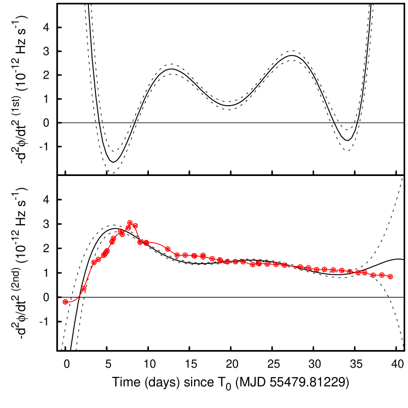
Figure 11: Black solid lines represent the second derivative of the 8-th order polynomial that best-fits the phases computed over the first (top panel) and the second harmonic (bottom panel). Dashed black curves mark the respective 1$\sigma$ confidence-level intervals. The change of sign of the second derivative of the best-fit polynomial is done to make the plotted function equal to the spin frequency derivative (see Eq. 4) and to facilitate comparison with light curve plotted in the top panel of Fig. 1 and reproduced in the bottom panel of this figure by using red circles (flux units are arbitrary).

The phase evolution is anyway far from being adequately fitted by a simple quadratic function and significant improvements of the description are successively obtained adding higher order terms, up to $N=8$. Considering that the phases computed over the two harmonic components have similar uncertainties, the quality of the modelling of the second harmonic phases ($\chi^{2}_{r}=1371.8/673=2.04$) is significantly better than for the first one ($\chi^{2}_{r}=4614.2/760=6.07$). Yet, these values indicate the presence of phase fluctuations which are not described by a polynomial expansion of a relatively low order. These fluctuations affect in a different manner the two harmonic components, though, and the trend followed by second harmonic phases is smoother than that followed by the phases computed over the first harmonic. To quantify this we evaluated the total RMS amplitude of the phase residuals with respect to the best-fitting polynomial as the squared sum of the statistical uncertainty on the phase measurement (which depends on the amplitude of the considered harmonic and on the count rate) and of the intrinsic phase noise, $\sigma^{2}_{k,rms}=\sigma^{2}_{k,stat}+\sigma^{2}_{k,noise}$, where $k$ is the harmonic number (see Hartman et al., 2008a, and references therein). By taking an average value for the statistical uncertainties one obtains that $\sigma_{1,noise}=0.055$ and $\sigma_{2,noise}=0.017$.

Table 1: Orbital parameters of J17480 obtained by modelling with Eq. 3 the phases computed on the first (left column) and on the second (central column) harmonic, together with the $\chi^{2}$ of the respective modelling. Uncertainties are given at 1$\sigma$ confidence level and were scaled by a factor $\sqrt{\chi_{r}^{2}}$ to take into account that $\chi^{2}>1$. The average between the values obtained considering the two harmonic components are listed in the rightmost column, with the uncertainties estimated conservatively such as to overlap the values indicated by the two components.

	1st harmonic	2nd harmonic	Average
a $\sin{i}$/c (lt-s)	2.4972(2)	2.4972(1)	2.4972(2)
Porb (s)	76588.4(1)	76587.92(6)	76588.1(3)
T∗ (MJD)	55481.78038(2)	55481.78052(1)	55481.78045(8)
e	$<6\times 10^{-4}$	$<1\times 10^{-4}$	$<2\times 10^{-4}$
$\chi^{2}$	5192.99/757	1436.74/668

An enhanced stability of the second harmonic phases is also indicated by the smooth trend followed by the second derivative of the best-fit polynomial, which equals in modulus the spin frequency derivative under the assumption that the NS spin is well tracked by the pulse phases (see Eq. 4). In the top and bottom panel of Fig. 11 we use black solid lines to plot the second derivative of the best-fitting function of the phases computed over the first and second harmonic, respectively. The curve computed over the first harmonic phases shows an oscillatory behaviour, especially towards the boundaries of the available data set. Such rapid variations of the spin up rate in absence of simultaneous swings of the X-ray light curve (the shape of which is reproduced in the bottom panel by using red circles; see also the top panel of Fig. 1) indicate how hardly the phase variations computed over the fundamental frequency component can be interpreted in terms of a variable torque acting onto the NS (see Sec. 4.3). This possibly indicates that the amplitude of the timing noise affecting the phases evaluated over this component is larger than the deviations from a parabolic trend due to the non constancy of the accretion torque, making the latter practically unmeasurable from this harmonic component. The phases computed over the second harmonic have instead a much smoother behaviour. The spin up rate increases during the first days reaching a maximum value of 2.8(1)$\times$10^-12 Hz s^-1 at the epoch 6.0$\pm$0.5 d since $T_{0}$, and subsequently smoothly decreases until it becomes ill-defined towards the boundary of the given data-set. Comparing the spin up rate calculated over the second harmonic phases to the X-ray light curve, it appears clear that the $\dot{\nu}$(t) curve follows much more closely the expected dependence on the instantaneous mass accretion rate.

These results indicate how the phases computed over the second harmonic are possiby a better tracker of the spin frequency of the NS. For this reason we use only this component to investigate if the observed behaviour is compatible with the accretion of Keplerian angular momentum of the matter at the inner edge of the disc (see next section). This choice is further motivated by the analogous behaviour observed in other accreting pulsars, where the second harmonic phases are often observed to be less affected by timing noise than the fundamental phases (see the Discussion, where a plausible explanation for such a behaviour is also proposed).

3.4 Torque modelling

To analyse whether the evolution of the pulse phases computed over the second harmonic can be described in terms of the torque imparted to the NS by the accreting matter, we assume that the torque depends on a power, $\beta$, of the mass accretion rate, $2\pi I_{*}\dot{\nu}\propto\dot{M}^{\beta}$, and that the mass accretion rate is well tracked by the X-ray luminosity, $\dot{M}=R_{*}L_{x}/\eta GM_{*}$, where $M_{*}$, $R_{*}$ and $I_{*}$ are the mass, radius and moment of inertia of the NS, respectively, and $\eta\simeq 1$ is the accretion efficiency. We thus consider a relation

$$\dot{\nu}(t)=\dot{\nu}(\bar{t})\left[\frac{L_{X}(t)}{L_{X}(\bar{t})}\right]^{\beta}$$ (5)

to express the dependence of the spin frequency derivative on the accretion luminosity. The bolometric accretion luminosity is estimated by extrapolating to the 0.05–150 keV energy band the best-fitting spectral models discussed in Sec. 3.1. The epoch $\bar{t}=\mbox{MJD}\>55487.63(6)=7.81(6)$ d since $T_{0}$, is the epoch at which the maximum luminosity, $L_{X}(\bar{t})=L_{max}=9.23(4)\times 10^{37}$ d${}_{5.9}^{2}$ erg s^-1 is attained.

Table 2: Frequency at the reference epoch and average spin frequency derivative obtained by fitting the first and second harmonic phases with the 8-th order polynomial defined by Eq. 3 (with $R_{orb}(t-T_{0})=0$), together with the relative $\chi^{2}$ and amplitudes of residuals (see text). Uncertainties are given at 1$\sigma$ confidence level and were scaled by $\sqrt{\chi_{r}^{2}}$ to take into account that $\chi^{2}_{r}>1$.

	1st harmonic	2nd harmonic
$\nu(T_{0})$ (Hz)	11.0448803(7)	11.0448797(5)
$<\dot{\nu}>$ (Hz s-1)	1.489(4)$\times 10^{-12}$	1.468(2)$\times 10^{-12}$
$\sigma_{rms}$	0.059	0.024
$\sigma_{stat}$	0.022	0.017
$\sigma_{noise}$	0.055	0.017
$\chi^{2}$	4614.2/760	1371.8/673

If the folding frequency is close to the actual spin frequency of the source and the frequency variation throughout the outburst is small, Eq. 2 can be expressed as

$$\phi(t)-\phi_{0}\simeq-\delta\nu\>(t-T_{0})-\int_{T_{0}}^{t}dt^{\prime}\int_{T_{0}}^{t^{\prime}}\dot{\nu}(t^{\prime\prime})\>dt^{\prime\prime}={}$$

$${}=-\delta\nu\>(t-T_{0})-\dot{\nu}(\bar{t})\>\int_{T_{0}}^{t}dt^{\prime}\int_{T_{0}}^{t^{\prime}}[L_{X}(t^{\prime\prime})/L_{X}(\bar{t})]^{\beta}\>dt^{\prime\prime},$$ (6)

where $\delta\nu=\nu(T_{0})-\nu_{f}$, and we have inserted the assumed dependency of the frequency derivative on X-ray luminosity (Eq. 5). One thus obtains a relation that can be used to fit the observed phase evolution depending on the parameters $\phi_{0}$, $\nu(T_{0})$, $\dot{\nu}({\bar{t}})$ and $\beta$.

In practise, we approximated the luminosity profile of the outburst $L_{X}(t)$ by using a natural smoothing cubic spline, which is plotted as a solid curve in panel (a) of Fig. 1. We then performed numerically the double integral of the function $L_{X}^{\beta}(t)$ for a set of values of $\beta$. We thus obtained a set of functions that were used to fit the observed evolution of the phases computed over the second harmonic. The best-fit is found for $\beta=1.07\pm 0.03$ with a $\chi^{2}=1574/672=2.34$, a value not far from the $\chi^{2}$ of the best-fitting 8-th order polynomial ($\chi^{2}_{r}=2.04$). This suggests a link between the phase variation computed over the second harmonic and the X-ray flux measured from the source. The best-fit values of the spin frequency at the beginning of the outburst $T_{0}$ and the spin frequency derivative at the outburst peak are, $\nu(T_{0})=11.044884819(6)$ Hz and $\dot{\nu}(\bar{t})=2.755(5)\times 10^{-12}$ Hz s^-1, respectively. The errors on the fitted parameters (quoted at the 1$\sigma$ confidence level) were evaluated by scaling the statistical errors by $\sqrt{\chi^{2}_{r}}$ to take into account the fact that $\chi^{2}_{r}>1$. The best-fitting model is plotted over measured data points, together with residuals, in Fig. 12.

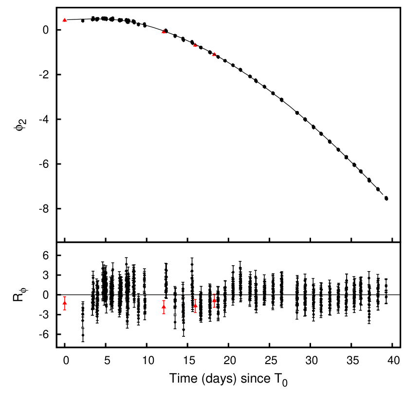
Figure 12: Best fitting model according to the physically-motivated torque model defined by Eq. 5 and 6 of the second harmonic phases (top panel), together with residuals in units of $\sigma$ (bottom panel).

To interpret the timing noise affecting the pulse phases observed from AMSP, Patruno et al. (2009) proposed that a large fraction of the unmodelled phase variability could be ascribed to a correlation between the phases and the X-ray flux. This would possibly reflect a dependence of the hot-spot location on the accretion rate. To check this hypothesis in the case of J17480 we substituted the double integral of the X-ray luminosity in Eq. 6 with a linear term in the X-ray luminosity, $k(t)=D\>L_{X}(t)$. The value of the chi-squared we obtain by fitting this model, $\chi^{2}_{r}=35.8$, clearly indicates that the observed phase variability cannot be explained in terms of such a correlation alone. Nevertheless a phase-flux correlation may still explain a small fraction of the phase variability, in addition to the accretion rate dependent torque. By adding $k(t)$ to Eq. 6 the chi-squared of the fit decreases in fact by $\Delta\chi^{2}=70$, with one degree of freedom less. The best-fitting parameters we obtain after the addition of this linear term to the model are, $\nu(T_{0})=11.044884842(6)$ Hz, $\dot{\nu}(\bar{t})=2.602(6)\times 10^{-12}$ Hz s^-1, $\beta=0.97\pm 0.04$ and $D=0.007(1)$ cycles s erg^-1.

4 Discussion

4.1 The energy spectrum

In Sec 3.1 we presented an analysis of the spectra accumulated by PCA on-board RXTE (2.5–30 keV), by XRT on-board SWIFT (1–10 keV) and by the JEM-X (4.5–25 keV) and ISGRI (20–150 keV) detectors on-board INTEGRAL. The phase-averaged continuum spectrum of J17480 is well described by thermal Comptonization. During the first few days of the outburst the temperature of the Comptonizing medium is $kT_{e}\lower 2.15277pt\hbox{$\;\buildrel>\over{\sim}\;$}10$ keV. It then decreases to values $\approx$ 3–3.5 keV as the source bolometric luminosity exceeds $\approx 3\times 10^{37}$ d${}_{5.9}^{2}$ erg s^-1, on MJD $\sim$ 55483, without showing further strong deviations from these values. Correspondingly, the optical depth increases from $\tau\approx\>$5 to 10. Unfortunately, because there is no observational coverage of the later stages of the outburst, it is not possible to ascertain the presence of a corresponding soft-to-hard transition and at which luminosity does it happen. The spectral transition observed during the outburst rise, as well as the softness of the spectrum characterising the emission of J17480 during most of the observations, is not typical of faster accreting pulsars. If compared with J17480, AMSP attain lower peak luminosities ($\;\buildrel<\over{\sim}\;$ few $\times 10^{36}$ erg s^-1), and their spectrum is generally described by Comptonization in a hotter and more optically transparent medium (with an electron temperature of $\approx$20-60 keV and optical depth $\approx$0.7-2.5, see Poutanen 2006, and references therein), not showing strong spectral variability during an outbursts. Only during the earliest observations, when the source was fainter than $\approx 3\times 10^{37}$ d${}_{5.9}^{2}$ erg s^-1, the spectrum observed from J17480 somewhat resembles those displayed by AMSPs. At larger luminosities instead, the observed spectrum is much more similar to those shown by brighter, non-pulsing, accretors (see, e.g., Barret & Olive, 2002). The decrease of the electron temperature of the Comptonized spectrum as the accretion luminosity increases can be interpreted in terms of an increase of the flux of soft photons which efficiently cool the Comptonizing region. In this context, it is worthwhile to note that based on the analysis of its correlated colour and aperiodic timing variability, Altamirano et al. (2010) and Chakraborty et al. (2011) concluded that this source transited from an Atoll-like to a Z-source like behaviour on MJD 55485, when the X-ray luminosity was close to attain its peak value. The hard to soft spectral evolution reported here is then part of a more general change of the properties of the accretion flow near the NS surface as the mass accretion rate increases.

4.2 The pulse profile shape

We presented in Sec. 3.2 an analysis of the 11 Hz pulses shown by J17480, based on PCA and XRT observations. The pulse shape can be modelled by using no more than two harmonic components. A major change of the pulse properties is observed at MJD $\sim$ 55483, while the source flux is increasing and the spectrum softening; the fractional amplitude of the first harmonic component suddenly decreases from $\sim 27\%$ to $\sim 2\%$, attaining a value of the same order of that of the second harmonic (see Fig. 4). The drop in the pulse strength is higher at soft energies, since the pulse amplitude becomes strongly energy dependent, showing a marked increase of the amplitude with the energy of the photons up to $30$ keV (see Fig. 6 and 8).

The shape of the pulses produced from the surface of an accreting rotating NS was modelled by a number of authors (see, e.g., Muno et al., 2002; Poutanen & Beloborodov, 2006; Cadeau et al., 2007; Lamb et al., 2009, and references therein) and depends on the geometry of the system (i.e., on the relative angles between the spin axis, the magnetic axis and the line of sight), on structural properties of the NS (mass, radius, shape and spin), on the beaming pattern of the emitted radiation, as well as on the size, temperature and brightness contrast of the accretion cap with respect to the rest of the NS surface. During most of the outburst the pulses shown by J17480 are of low amplitude (few per cent) and simple, similar to the majority of AMSP (see Lamb et al. 2009, L09 hereafter). However, the amplitude decrease by more than a factor of 10 taking place on MJD $\sim$ 55483 on a timescale of less than one day (see Fig. 4), indicates how some of the properties that determine the pulse amplitude must have changed significantly as the X-ray luminosity was increasing during the outburst rise. Variations of the pulse amplitude of a similar amount were already observed from a number of AMXPs; swings from 3 to 25 per cent have been observed from XTE J1807–294 (Zhang et al., 2006), and from 4 to 14 per cent in the case of SAX J1808.4–3658 (Hartman et al., 2008b). In those cases, though, the amplitude variations were closely related to flaring episodes during the outbursts. On the other hand, the decrease of the pulsed fraction shown by J17480 is step-like and no significant correlation holds between the pulsed fraction and the X-ray flux afterwards. In the following a number of hypotheses to account for the observed variation of the pulse properties during the outburst rise is discussed. Unfortunately, a coverage of the later stages of the outburst decays is not available, preventing to investigate if a similar transition happens as the source dims and at which luminosity would it take place.

A change of the spot size is hardly the main driver of the observed pulse fraction decrease; the spot size is in fact expected not to vary by more than $\sim 10\%$ as the luminosity doubles, and the results obtained by Muno et al. (2002) and L09 show how the dependence of the pulse amplitude on the spot size is much weaker than it would be needed to explain the observed variation.

Pulse amplitude variations can be explained in terms of movements of the hot spot location on the NS surface, possibly caused by the in-falling matter getting attached to a different set of magnetic field lines. An increase of the spot latitude can be particularly efficient in decreasing the pulse amplitude, especially if the angle between the magnetic and the spin axis is small. This was invoked by L09 to explain some of the properties of the pulses shown by AMSPs, such as small and variable amplitudes, and unstable pulse phases. According to their results a change of roughly $15-30^{\circ}$ of the spot latitude towards the magnetic pole would be able to produce an amplitude decrease of the order of that observed from J17480. Further, under the hypothesis that the two spots on the NS surface are antipodal, a re-sizing, or shift, of the impact region of the in-falling matter on the NS could increase the fraction of rotational phases during which both spots on the NS surface become visible. This would indeed contribute to explain the observed reduction of the pulse amplitude and strengthening of the second harmonic amplitude relative to the first one. Although this scenario is then in principle able to explain the decrease of the pulse amplitude integrated over the entire PCA energy-band, it gives no sufficient clues for the simultaneous change of the energy dependence of the pulse profile shape.

An amplitude variation of the order of that observed could also be produced by a significant change of the angular distribution of the photons that reach the observer, possibly triggered by the source luminosity crossing a certain threshold level (see, e.g., Parmar et al., 1989, who interpreted as such the luminosity dependent changes of the pulse profile of the 42 s high-field pulsar, EXO 2030+375). While the radiation transmitted through a slab is strongly peaked along the normal to the NS surface, scattered radiation is expected to peak at intermediate angles, in a fan-like emission pattern (e.g. Sunyaev & Titarchuk, 1985). The relations given by Poutanen & Beloborodov (2006, see, e.g., Eq. 51 and 61) show that an amplitude change of the same order of that observed can be reproduced if the angular distribution of the emitted photons switches from being strongly peaked along the normal [$I(\alpha)\propto(1+h\cos{\alpha})$, where $\alpha$ is the angle to the normal and $h\simeq$ 2], to a fan like distribution (h$\simeq$ -1). However, such a drastic change of the pattern of the emitted radiation would produce a change of $\sim 0.5$ in the pulse phase, which is not observed.

The decrease of the pulse amplitude shown by J17480, as well as its spectral hardening, take place roughly simultaneously to the spectral softening of the phase-averaged emission discussed in the previous section. It is then intriguing to explain these transitions in terms of a variation of the properties of the matter flow close to the NS surface. The observed behaviour would be in fact explained if a large fraction of the source luminosity, and in particular its softer part, becomes not pulsed during the outburst rise. This could happen because the inner rim of the disc approaches the NS surface, with an increased part of the disc non-pulsed emission falling in the considered energy band, and/or because an increasing fraction of the in-falling matter is not channelled to the magnetic poles, but rather accretes more evenly at the NS equator in a sort of optically thick boundary layer. The properties of the phase-averaged spectrum presented in Sec. 3.1 would favour the latter hypothesis. The possibility that not all the plasma from the accretion disc is lifted off by magnetic field lines at the magnetospheric boundary, with a fraction penetrating between the magnetic field lines via a Rayleigh-Taylor instability or because of incomplete coupling of the plasma and the field lines was studied by, e.g., Spruit & Taam (1990) and Miller et al. (1998, see references therein, also). Recent 3D MHD simulations of disc accretion onto a magnetised NS performed by Romanova et al. (2008) showed how a transition to this twofold accretion channel may take place when the mass accretion rate becomes larger than $\simeq 0.1(B/10^{9}\mbox{G})^{2}\dot{M}_{Edd}$. Above this level it could then be that only a fraction $\sim 10$% of the accreted mass is channelled to the poles. The rest would be accreted preferentially at the star equatorial belt producing the observed optically thick Comptonized component, reminiscent of emission from non pulsing NS in LMXB. The hardening of the energy dependence of pulse amplitude would be naturally explained by this scenario. The pulsed emission originating from the polar caps is in fact expected to be harder than the non-pulsed emission produced in a denser equatorial boundary layer. Interestingly, an increase of the pulse amplitude with energy similar to that of J17480 was observed only from three AMSPs, SWIFT J1756.9-2508 (Patruno et al., 2010), Aql X-1 (Casella et al., 2008) and SAX J1748.9-2021 (Patruno et al., 2009), the last two being sources that showed pulsations only intermittently. To conclude, it has to be noted that a pulse amplitude increase at energies $\lower 2.15277pt\hbox{$\;\buildrel>\over{\sim}\;$}50$ keV was also observed by Falanga & Titarchuk (2007) from IGR J00291+5934. Since it concerned high photon energies, the authors interpreted such an increase as due to the decrease of the electron scattering cross section with energy. This effect clearly does not explain the pulse amplitude properties observed from J17480, as well as from the other mentioned sources, since the pulse amplitude is observed to increase even at low ($\lower 2.15277pt\hbox{$\;\buildrel>\over{\sim}\;$}2.5$ keV) energies.

4.3 Phase evolution.

We presented in Sec. 3.3 and 3.4 an analysis of the temporal evolution of the phase of the pulse shown by J17480 during its 2010 outburst, based on the whole data set available of PCA and XRT observations. The results obtained confirm the earlier finding that the NS in this system accelerates while it accretes mass (P11). While the analysis performed on the phases computed over the first and second harmonic gives slightly different values of the average frequency derivative, a value of $<\dot{\nu}>=1.48(2)\times 10^{-12}$ Hz $s^{-1}$ encompasses both estimates.

The observed frequency derivative of the signal emitted by a pulsar is the sum of the intrinsic change of the NS spin and of the acceleration of the pulsar with respect to the observer. While the apparent spin frequency derivative due to centrifugal acceleration ($\lower 2.15277pt\hbox{$\;\buildrel<\over{\sim}\;$}\nu\mu^{2}d/c\simeq 1.4\times 10^{-18}$ d_5.9 Hz s^-1, Shklovskii 1970, where $\mu=85\pm 10$ km s^-1 is the velocity of the proper motion of Terzan 5 estimated by Ferraro et al. 2009) and to galactic acceleration ($\simeq 2\times 10^{-17}$ Hz s^-1, obtained by inserting the galactic coordinates of J17480 in the relation given by Damour & Taylor 1991) can be safely neglected, the acceleration of the pulsar in the gravitational field of the cluster can in principle have a larger effect. Phinney (1993) estimated the maximum acceleration along the line of sight for an object located at a projected angular distance $\theta_{\bot}$ from the cluster centre as $1.1\>\nu\>G\>M_{cyl}(<\theta_{\bot})/(c\>\pi\>d^{2}\>\theta_{\bot}^{2})$ Hz s^-1, where $M_{cyl}(<\theta_{\bot})$ is the mass within a projected distance smaller than $d\>\theta_{\bot}$ from the cluster centre. Considering the cluster parameters estimated by Lanzoni et al. (2010) from the surface brightness profile of Terzan 5 (core and tidal radius of $9^{\prime\prime}$ and $277^{\prime\prime}$, respectively, and a total bolometric luminosity of $8\times 10^{5}$ L_☉) and the projected distance of the pulsar from the cluster centre ($\bar{\theta}_{\bot}\simeq 4^{\prime\prime}$) to integrate the King density profile (King, 1962) up to $\theta_{\bot}$, yields a mass $M_{cyl}(<\bar{\theta}_{\bot})\simeq 5\times 10^{4}$ M$\sun$, where a mass-to-light ratio of 3 was assumed. Inserting such a value in the relation given above yields an apparent frequency derivative of $\simeq 6\times 10^{-15}$ Hz s^-1, which is more than two orders of magnitude lower than the observed derivative and can be safely neglected.

The average derivative of the signal frequency is compatible with the average acceleration imparted to the NS by the accretion of the Keplerian angular momentum of disc matter. By considering only this torque, $N_{0}$, and assuming that the X-ray luminosity tracks the mass accretion rate (see Sec. 3.4), the expected spin frequency derivative of an accreting NS is

$$\dot{\nu}=\frac{N_{0}}{2\pi I_{*}}=\frac{\sqrt{GM_{*}}}{2\pi I_{*}}\dot{M}\sqrt{R_{in}}=\frac{R_{*}}{2\pi I_{*}\eta\sqrt{GM_{*}}}\sqrt{R_{in}}\;L_{X},$$ (7)

where $R_{in}$ is the inner disc radius. By inserting the measured value of $<\!\dot{\nu}\!>$ in Eq. 7, an estimate of the average inner disc size of $<\!R_{in}\!>\simeq 64\;\eta^{2}\;R_{*,10}^{-2}\;M_{*,1.4}\;I_{45}^{2}(<\!L_{37}\!>/\>5)^{-2}$ km is obtained, where $R_{*,10}$ is the NS radius in units of 10 km, $M_{*,1.4}$ the NS mass in units of 1.4 M_⊙, $I_{*,45}$ the NS moment of inertia in units of $10^{45}$ g cm² and $L_{37}$ is the accretion luminosity in units of $10^{37}$ erg s^-1 . Such a value is clearly compatible with the upper and lower bounds set by the presence of pulsations, $R_{*}<R_{in}\lower 2.15277pt\hbox{$\;\buildrel<\over{\sim}\;$}R_{C}$, where $R_{C}=338$ $M_{*,1.4}^{1/3}$ km is the corotation radius around the NS in J17480 (P11).

The analysis presented in Sec. 3.3 shows that a constant frequency model is not compatible with the observed evolution of the phases of J17480. Yet, values of the reduced $\chi^{2}$ in excess of one are obtained even if an 8-th order polynomial expansion is considered as a model, indicating the presence of timing noise. Before discussing the results obtained by modelling the observed phase evolution with a physically-motivated torque model, the influence of such a noise on the phase determination has to be discussed.

Noisy variability in the phases of accreting pulsars is not new and manifests itself through the presence of unmodelled phase residuals with respect to the considered timing solution. In particular, it affects the pulses shown by AMSPs and it was subject of a profound analysis and discussion (see, e.g., Burderi et al., 2006; Papitto et al., 2007; Hartman et al., 2008a; Riggio et al., 2008a; Lamb et al., 2009; Patruno et al., 2009, and references therein). The analysis of the temporal evolution of the phases of the pulse profile shown by a pulsar allows in principle the most accurate possible knowledge of the rotational evolution of the NS. However, irregular variability of the pulse phases not related to intrinsic spin changes of the NS hinders this possibility. Indeed, this is particularly troublesome for transiently accreting pulsars such as AMSP which are expected to experience relatively small frequency variations during their outbursts. In those cases the amplitude of the phase variability induced by timing noise can be comparable to that produced by a spin frequency derivative. This is certainly not the case of J17480, since, despite the presence of timing noise, the pulse phase is observed to perform more than one phase cycle across the outburst (see Fig. 9 and 10). This source can be therefore regarded as a particularly relevant case to the study of accreting pulsars, since the the contributions of timing noise and of the rotational evolution to the pulse phase variations may be disentangled to some extent.

An evident property of the phase noise of J17480 is that affects roughly three times more weakly the phases computed over the second harmonic than those of the fundamental. Together with the much easier description of the evolution of the second harmonic phases in terms of a physically plausible torque model (see Sec. 3.4 and in the following), this provides an observational indication of how the second harmonic component might be a better tracer of the spin frequency evolution of an accreting pulsar. The enhanced stability of the second harmonic component with respect to the fundamental was already observed in a number of AMSPs. Sudden jumps of the first harmonic phases not accompanied by a corresponding variation of the second harmonic were observed during a couple of outbursts of SAX J1808.4–3658 (Burderi et al., 2006; Hartman et al., 2009), while during other outbursts a comparable amount of noise affected the two harmonic components (Hartman et al., 2008a). A similar phenomenology is also observed from SWIFT J1749.4–2807 (Papitto et al., in prep.). Further, in a couple of cases (XTE J1807–295, Riggio et al. 2008b; IGR J17511-3057, Riggio et al. 2011) the noise affecting the second harmonic component was found to be significantly milder than that affecting the fundamental frequency; moreover, only by modelling the second harmonic component a physically plausible timing solution could be proposed for these systems. While the different stability of the various harmonic components was taken into account by Hartman et al. (2008a) to derive a minimum variance estimator for the phases of the pulse profile, not many attempts have been made to explain such a different behaviour of the phases computed over different Fourier components. If the observed variability of the pulse amplitudes and phases is due to irregular motion of the spot on the NS surface (L09) similar shifts should be observed in all the Fourier components. This has been observed and interpreted as such only in the case of XTE J1814-338 (Papitto et al., 2007; Watts et al., 2008). While it could well be that substantial changes in the spot-shape or in the radiation-pattern of the emitted radiation determine a change of the pulse shape, this does not seem to naturally explain the enhanced stability of the second harmonic observed in a number of cases, and why only the use of the second harmonic phases as a tracker of the NS spin frequency generally produces results in accordance with theoretical expectations.

A simple model proposed by Riggio et al. (2011) explains a similar behaviour in terms of modest variations of the relative intensity received by the two polar caps onto the NS surface, if the geometrical properties of the system make the signal coming from the two spots of similar amplitude. It is assumed that the pulse profile observed from an accreting pulsar is given by the sum of two signals with a similar harmonic content, emitted by two nearly antipodal spots on the NS surface ($\Delta\lambda\approx\pi$, $\Delta\gamma\approx 2\gamma$, where $\gamma$ and $\lambda$ are the latitude and longitude of the primary spot, respectively, and $\Delta\lambda$ and $\Delta\gamma$ are the differences between the coordinates of the two spots), as it is the case if the magnetic field has a dipolar shape. The sum of the two signals (the total profile) will be the result of a destructive interference for what concerns the fundamental harmonic of the signal, since it is the sum of two signals with a phase difference of $\approx\pi$. A constructive interference develops instead for the second harmonic of the total profile, since it is the sum of two signals with the same phase. The destructive interference regarding the fundamental frequency leads to (i) small values of the pulsed fraction of the first harmonic component, possibly comparable to that of the second harmonic, and (ii) large swings of the phase of the fundamental of the total profile due to modest variations of the relative intensity of the signals emitted by the two caps. The magnitude of these effects is the largest when the spots on the NS surface are exactly antipodal and produce signals that are observed at a similar amplitude. In this case swings up to 0.5 phase cycles can be shown by the phase computed over the fundamental frequency of the observed profile, without correspondingly large variations of the phase of the second harmonic. The maximum variability of the phase of the first harmonic component, as well as the maximum reduction of its amplitude, is obtained when the intensity of the signals observed from the two magnetic caps is very similar. This happens if the system is viewed nearly edge on and/or if the rotator is nearly orthogonal, that is with an angle between the spin and the magnetic axes of $\approx 90^{\circ}$. Under these assumptions such a simple model can reproduce phase movements of the order of those observed from J17480, as well as the enhanced stability observed from the second harmonic phases, in terms of variations of few per cent of the ratio between the intensity observed by the two spots. A thorough quantitative discussion of how this model applies to this, and other cases is deferred to a dedicated paper (Riggio et al., in prep.).

In addition to the smaller residuals with respect to phenomenological models, an enhanced stability of the second harmonic phases is also indicated by the possibility of describing their behaviour by using a physically plausible model. In Sec. 3.3 and 3.4 we showed how the description of the pulse phases determined using the second harmonic component is significantly improved by assuming that the frequency derivative of the signal depends on a power close to one of the X-ray flux. The descritption of the pulse phases is further improved by the assumption of a phase-flux correlation such as that proposed by Patruno et al. (2009), even if by a much lesser extent. On the other hand, the spin frequency derivative evaluated by considering the first harmonic phases shows oscillations that are not correlated with the X-ray luminosity.

Under the hypothesis that the second harmonic phases are a good tracker of the NS spin, we can infer some of the properties on the size of the inner radius of the accretion disc and on its dependence on the X-ray luminosity. To this end we consider the results presented in Sec. 3.4, where the phases of the second harmonic were fitted by assumung a relation, $\dot{\nu}\propto L_{X}^{\beta}$, for the dependency of the spin-up torque on the accretion luminosity. According to standard accretion disc theory, the angular momemtum is transferred from the disc matter to the magnetosphere at the inner disc radius $R_{in}$. In turn, the size of the inner edge of the disc is determined by evaluating where the stresses exerted by the magnetic field lines on the accreting plasma become dominant with respect to the viscous stresses, that grant angular momentum redistribution in the disc far from the magnetosphere (see, e.g., Ghosh, 2007, and references therein). The location of the inner disc radius is usually expressed as a fraction $\xi$ of the Alfven radius evaluated in the case of spherical symmetric accretion

$$R_{in}=71\>\xi\>\eta^{2/7}\>M_{*,1.4}^{1/7}\>R_{*,10}^{-2/7}\>L_{37}^{-2/7}\>\mu_{27}^{4/7}\>\mbox{km}.$$ (8)

Here, $\mu_{27}$ is the magnetic-dipole moment in units of $10^{27}$ G cm³, and the factor $\xi$ is determined by capability of the field lines to thread the disc matter, and by the magnetic pitch, which in turn is limited by the reconnection-mechanisms of the field lines through the disc (Ghosh & Lamb 1979; Wang 1996, who quote values of $\xi$ between 0.5 and 1, respectively; see also the discussion of these models given by Bozzo et al. 2009). Inserting this expression in Eq. 7, it can be seen that the spin frequency derivative is expected to scale as $\dot{\nu}\propto L_{X}^{6/7}$, if the only relevant torque is that exerted by matter orbiting in a Keplerian disc.

The dependence on the X-ray luminosity of the spin frequency derivative evaluated from the phases of the second harmonic shown by J17480, $\beta=1.07\pm 0.03$, is steeper than what is predicted by standard accretion theory. Values of $\beta$ close to unity were already reported by Bildsten et al. (1997) for the 0.47 s accreting pulsar in a LMXB, GRO J1744–28 ($\beta=0.957\pm 0.026$) and the 105 s high field pulsar, A0535+26 ($\beta=0.951\pm 0.026$), as well as by Parmar et al. (1989) for the 42 s high field accreting pulsar, EXO 2030+375 ($\beta=1.21\pm 0.13$). Expressing the dependence of the inner disc radius on the accretion luminosity as $R_{in}\propto L_{X}^{-\alpha}$, the estimate of $\beta$ found for J17480 translates in a value of $\alpha=2(1-\beta)=-0.14\pm 0.06$. A negative value of $\alpha$ would imply a positive correlation of the inner disc radius with the X-ray luminosity, which seems unlikely on physical grounds. On the other hand, a value close to zero indicates a very weak, if any, dependence of the inner disc radius on the accretion luminosity. A similar result, $\beta=0.97(4)$ [$\alpha=0.06(8)$], is obtained when adding to the model used to fit the phases a term depending linearly on the X-ray luminosity.

By considering the value of the spin up torque, $\dot{\nu}(\bar{t})=2.755(5)\times 10^{-12}$ Hz s^-1, attained when the X-ray luminosity reached its peak value, $L_{X}(\bar{t})=9.23(4)\times 10^{37}$ d${}_{5.9}^{2}$ erg s^-1, and assuming that the NS accretes the Keplerian angular momentum of matter at the inner disc boundary $R_{in}$ (Eq. 7), the inner edge of the disc is estimated as $R_{in}(\bar{t})=65(1)\>\eta^{2}I_{*,45}^{2}\>M_{*,1.4}\>R_{*,6}^{-2}\>d_{5.9}^{-4}$ km. A slightly smaller estimate, $\simeq 58$ km, is obtained if the value of the frequency derivative obtained after adding a linear term in the X-ray luminosity to the model used to fit the phases, $\dot{\nu}(\bar{t})=2.602(6)\times 10^{-12}$ Hz s^-1, is considered. The error on the distance ($\simeq 8\%$ of its estimate) is the largest source of uncertainty on the disc size measure. By taking it into account, the estimate of $R_{in}(\bar{t})$ lies between 47 and 93 km (1$\sigma$ confidence level). Inserting the measured values of $R_{in}$ and $L_{max}$ in Eq. 8 yields to an estimate of the magnetic-dipole moment, $\mu_{27}=2.6(2)\>\xi^{-7/4}\>d_{5.9}^{-6}\>I_{*,45}^{7/2}\>R_{*,10}^{-3}\>M_{*,1.4}^{3/2}\>\eta^{-15/4}$, which has a similarly large uncertainty and for $\xi\simeq 0.5$ varies between 5 and 16. A magnetic surface flux density between $\sim 5\times 10^{9}$ and $\sim 1.5\times 10^{10}$ G is therefore likely.

Since J17480 is a relatively slow pulsar, a coupling between magnetic field lines and plasma rotating in the accretion disc beyond the inner disc radius transfers additional angular momentum to the NS. To take into account this effect, the torque on the NS can be expressed as

$$N\approx 1.4\>N_{0}\>\frac{1-\omega_{S}/\omega_{C}}{1-\omega_{S}}$$ (9)

(Ghosh & Lamb, 1979). Here, $\omega_{S}=2\pi\nu\sqrt{R_{in}^{3}/GM}$ is the fastness parameter while $\omega_{C}$ is the critical fastness, which takes values between 0.35 and 1 depending on the description of the interaction between the field and the disc (Ghosh & Lamb, 1979; Wang, 1996). Taking the value of $\omega_{C}=0.6$ obtained by Romanova et al. (2002) from numerical simulations, and equating the observed torque to Eq. 9, the estimate of the inner disc radius at $\bar{t}$ reduces to roughly half of the estimate given above, $R_{in}\simeq 36\>d_{5.9}^{-4}$ km, where only the steep dependence on the distance was made explicit. The modelling of the phases of the second harmonic with a phisically plausible torque model yields therefore a value of the inner disc radius compatible with the estimate given by Miller et al. (2011) on a spectroscopic basis, $41(5)\>M_{*,1.4}$ km; the latter value was obtained by interpreting in terms of relativistic broadening the profile of the iron K-$\alpha$ line detected in the spectrum of the source observed by Chandra on 55493.445, (13.632 d since $T_{0}$), when the X-ray luminosity was a factor $\approx 0.6$ lower than at the peak. Still, these estimates appear slightly larger than the inner disc radius implied by the observation of a QPO at 815 Hz during the outburst peak (Altamirano et al., 2010), $R_{in}\simeq 19\>M_{*,1.4}$ km, if such a feature is interpreted in terms of a Keplerian orbital frequency. Given the steep dependence of our inner disc radius estimate on the distance to the source, the size given by the Keplerian interpretation of the QPO would be reconciled with the value indicated by the torque analysis presented here if a distance of $\lower 2.15277pt\hbox{$\;\buildrel>\over{\sim}\;$}7$ kpc to the Globular cluster is assumed. A similar value is marginally compatible with the most recent determination ($5.9\pm 0.5$ kpc), though it has to be noted that heavy, differential reddening affecting observations of this Globular cluster make the determination of its distance somewhat problematic (Lanzoni et al., 2010, and references therein).

Table 3: Best-fitting parameters of the spectral continuum evaluated from the 2.5–30 keV spectra observed by PCA on-board RXTE. Columns are: Observation ID (labels refer to the groups of observations defined in text); Start time of the observation (MJD since $T_{0}$ = MJD 55479.81229); End time of the observation (MJD since $T_{0}$); Exposure (ks); $kT_{e}$ (keV); $\tau$; $kT_{S}$ (keV); Unabsorbed flux in the 2.5–25 keV band ($10^{-8}$ erg cm^-2 s^-1); Bolometric luminosity calculated by extrapolating the best-fitting model to the 0.05–150 keV energy band ($d_{5.9}^{2}\>10^{37}$ erg cm^-2 s^-1); Reduced chi-squared of the fit. The quoted errors are evaluated at the 90% confidence level on each parameter ($\Delta\chi^{2}=2.706$).

ObsID	Tstart (MJD)	Tend (MJD)	Expo (ks)	kTe (keV)	$\tau$	kTS (keV)	F($10^{-8}$ erg cm2 s-1)	L ($d_{5.9}^{2}\>10^{37}$ erg s-1)	$\chi^{2}$/dof
95437-01-01-00 – Obs. [B]	2.1964	2.2328	2.3	$6.7_{-0.2}^{+0.2}$	$8.22_{-0.09}^{+0.07}$	$0.80_{-0.04}^{+0.04}$	0.340(2)	1.91(4)	65.1/49
95437-01-02-00	3.3740	3.5506	7.5	$3.7_{-0.03}^{+0.04}$	$9.57_{-0.03}^{+0.06}$	$0.840_{-0.006}^{+0.03}$	0.966(2)	4.81(2)	51.7/49
95437-01-02-01 – Obs. [C]	3.9028	4.0665	8.2	$3.62_{-0.03}^{+0.01}$	$9.43_{-0.10}^{+0.02}$	$0.85_{-0.05}^{+0.01}$	1.033(2)	5.14(2)	57.9/49
95437-01-03-00	4.6214	4.6506	1.4	$3.36_{-0.02}^{+0.02}$	$9.94_{-0.02}^{+0.02}$	$0.81_{-0.01}^{+0.01}$	1.122(3)	5.62(3)	46.7/49
95437-01-03-01	4.7560	4.7895	1.4	$3.34_{-0.03}^{+0.02}$	$9.78_{-0.02}^{+0.02}$	$0.82_{-0.01}^{+0.02}$	1.142(3)	5.73(3)	50.9/49
95437-01-03-02	4.8162	4.8549	2.4	$3.34_{-0.04}^{+0.02}$	$9.62_{-0.04}^{+0.12}$	$0.83_{-0.02}^{+0.05}$	1.170(3)	5.87(4)	58.0/49
95437-01-03-03	4.9432	5.1165	8.0	$3.33_{-0.01}^{+0.01}$	$9.39_{-0.01}^{+0.01}$	$0.828_{-0.006}^{+0.005}$	1.201(2)	6.06(2)	61.5/49
95437-01-04-00	5.6019	5.7049	3.5	$3.22_{-0.06}^{+0.01}$	$8.82_{-0.06}^{+0.04}$	$0.88_{-0.07}^{+0.02}$	1.404(3)	7.11(3)	57.6/49
95437-01-04-01	5.7347	5.9014	6.1	$3.18_{-0.04}^{+0.04}$	$8.97_{-0.06}^{+0.09}$	$0.86_{-0.02}^{+0.03}$	1.473(3)	7.49(4)	60.1/49
95437-01-05-00	6.6486	6.7514	4.2	$2.97_{-0.01}^{+0.01}$	$8.31_{-0.07}^{+0.02}$	$0.90_{-0.02}^{+0.01}$	1.613(3)	8.29(3)	62.9/49
95437-01-05-01	6.7743	6.9471	8.9	$2.905_{-0.008}^{+0.007}$	$8.56_{-0.01}^{+0.02}$	$0.862_{-0.004}^{+0.004}$	1.528(3)	7.94(3)	66.6/49
95437-01-06-000	7.4932	7.7473	8.8	$2.938_{-0.008}^{+0.008}$	$8.29_{-0.01}^{+0.01}$	$0.853_{-0.004}^{+0.004}$	1.658(3)	8.68(3)	47.5/49
95437-01-06-00 – Obs. [D]	7.7527	7.8804	4.7	$3.001_{-0.01}^{+0.009}$	$8.69_{-0.01}^{+0.02}$	$0.829_{-0.005}^{+0.004}$	1.771(3)	9.23(4)	55.3/49
95437-01-07-00	8.3375	8.5604	7.0	$3.08_{-0.2}^{+0.02}$	$8.35_{-0.10}^{+0.05}$	$0.84_{-0.02}^{+0.02}$	1.704(3)	8.89(4)	32.1/49
95437-01-07-01	8.9969	9.0577	2.3	$2.73_{-0.02}^{+0.06}$	$7.88_{-0.07}^{+0.10}$	$0.88_{-0.02}^{+0.02}$	1.334(3)	7.06(3)	57.0/49
95437-01-08-00	9.7167	9.8493	5.2	$2.93_{-0.02}^{+0.009}$	$7.97_{-0.02}^{+0.01}$	$0.886_{-0.004}^{+0.003}$	1.348(3)	7.02(3)	42.8/49
95437-01-10-01	12.3310	12.4341	4.5	$3.18_{-0.01}^{+0.01}$	$8.86_{-0.01}^{+0.01}$	$0.799_{-0.005}^{+0.005}$	1.214(2)	6.30(3)	47.2/49
95437-01-10-02	13.4540	13.5523	4.2	$3.05_{-0.4}^{+0.08}$	$8.3_{-0.4}^{+0.2}$	$0.97_{-0.05}^{+0.01}$	1.123(3)	5.63(5)	52.1/47
95437-01-10-03	14.4310	14.5554	4.3	$2.84_{-0.01}^{+0.07}$	$9.95_{-0.01}^{+0.07}$	$0.916_{-0.010}^{+0.004}$	1.129(2)	5.63(2)	60.7/49
95437-01-10-04	15.5345	15.5736	2.4	$3.19_{-0.02}^{+0.02}$	$9.28_{-0.04}^{+0.02}$	$0.81_{-0.01}^{+0.02}$	1.089(2)	5.57(3)	65.0/49
95437-01-10-07	15.6012	15.6582	2.5	$2.98_{-0.009}^{+0.01}$	$9.85_{-0.01}^{+0.08}$	$0.86_{-0.01}^{+0.04}$	1.102(2)	5.55(3)	40.4/49
95437-01-10-05	16.5797	16.7062	4.8	$2.95_{-0.1}^{+0.04}$	$10.2_{-0.8}^{+0.1}$	$0.94_{-0.02}^{+0.03}$	1.107(2)	5.45(2)	57.7/49
95437-01-10-06	17.6991	17.8117	4.7	$2.908_{-0.006}^{+0.006}$	$10.98_{-0.01}^{+0.01}$	$0.873_{-0.004}^{+0.002}$	1.059(1)	5.23(1)	80.3/49
95437-01-11-07	18.6880	18.7110	1.3	$2.88_{-0.02}^{+0.01}$	$11.41_{-0.80}^{+0.02}$	$0.8_{-0.1}^{+0.1}$	1.016(3)	5.10(3)	49.4/49
95437-01-11-00	18.7371	18.7903	2.8	$3.00_{-0.01}^{+0.01}$	$10.45_{-0.02}^{+0.02}$	$0.871_{-0.009}^{+0.006}$	1.006(2)	5.00(2)	55.1/49
95437-01-11-01	19.5358	19.6465	4.2	$3.11_{-0.01}^{+0.01}$	$10.09_{-0.04}^{+0.03}$	$0.89_{-0.02}^{+0.08}$	0.997(2)	4.93(2)	53.2/49
95437-01-11-02	20.5158	20.6291	4.3	$3.24_{-0.02}^{+0.01}$	$10.01_{-0.06}^{+0.02}$	$0.88_{-0.02}^{+0.02}$	0.993(2)	4.92(2)	54.4/49
95437-01-11-03	21.4310	21.5443	4.2	$3.35_{-0.01}^{+0.02}$	$9.62_{-0.02}^{+0.02}$	$0.885_{-0.006}^{+0.006}$	0.990(2)	4.90(2)	67.2/49
95437-01-11-04	22.5923	22.6971	5.4	$3.48_{-0.08}^{+0.01}$	$9.09_{-0.09}^{+0.02}$	$0.87_{-0.02}^{+0.01}$	0.921(2)	4.59(2)	79.7/49
95437-01-11-05	23.3173	23.3447	2.1	$3.32_{-0.03}^{+0.02}$	$10.03_{-0.03}^{+0.02}$	$0.84_{-0.04}^{+0.02}$	0.952(2)	4.73(3)	39.7/49
95437-01-11-08	23.3817	23.4403	2.4	$3.34_{-0.07}^{+0.03}$	$9.75_{-0.22}^{+0.09}$	$0.86_{-0.02}^{+0.02}$	0.942(2)	4.68(3)	72.8/49
95437-01-11-06	24.3567	24.4812	5.4	$3.39_{-0.04}^{+0.01}$	$9.66_{-0.05}^{+0.06}$	$0.88_{-0.01}^{+0.03}$	0.939(2)	4.64(2)	54.5/49
95437-01-12-00	25.4164	25.5256	4.4	$3.36_{-0.01}^{+0.01}$	$9.88_{-0.02}^{+0.02}$	$0.876_{-0.006}^{+0.006}$	0.931(2)	4.60(2)	61.3/49
95437-01-12-01	26.4454	26.5701	5.6	$3.48_{-0.02}^{+0.02}$	$9.37_{-0.05}^{+0.03}$	$0.91_{-0.03}^{+0.02}$	0.916(2)	4.51(2)	80.8/49
95437-01-12-03	28.3430	28.4708	5.7	$3.45_{-0.05}^{+0.03}$	$9.51_{-0.11}^{+0.07}$	$0.92_{-0.05}^{+0.02}$	0.880(2)	4.32(2)	62.9/49
95437-01-12-04	29.3238	29.4527	5.6	$3.38_{-0.01}^{+0.01}$	$10.10_{-0.01}^{+0.02}$	$0.851_{-0.007}^{+0.010}$	0.854(2)	4.23(2)	60.8/49
95437-01-12-05	30.3362	30.4527	4.7	$3.39_{-0.01}^{+0.04}$	$9.76_{-0.02}^{+0.03}$	$0.854_{-0.005}^{+0.030}$	0.810(2)	4.03(2)	60.7/49
95437-01-12-06	31.2838	31.3888	5.9	$3.46_{-0.05}^{+0.02}$	$9.61_{-0.10}^{+0.04}$	$0.90_{-0.05}^{+0.02}$	0.821(2)	4.05(2)	70.0/49
95437-01-13-00	32.3427	32.4471	4.8	$3.46_{-0.09}^{+0.03}$	$9.58_{-0.30}^{+0.04}$	$0.90_{-0.07}^{+0.02}$	0.808(2)	3.98(2)	54.6/49
95437-01-13-01	33.3886	33.4799	4.9	$3.47_{-0.07}^{+0.02}$	$9.51_{-0.10}^{+0.04}$	$0.92_{-0.06}^{+0.02}$	0.801(2)	3.94(2)	80.6/49
95437-01-13-02	34.3547	34.4604	5.4	$3.44_{-0.1}^{+0.04}$	$9.74_{-0.10}^{+0.07}$	$0.90_{-0.04}^{+0.02}$	0.772(1)	3.80(2)	69.4/49
95437-01-13-03	35.3356	35.4578	6.0	$3.46_{-0.05}^{+0.03}$	$9.76_{-0.10}^{+0.06}$	$0.89_{-0.04}^{+0.01}$	0.751(2)	3.70(2)	78.3/49
95437-01-13-04	36.1199	36.2499	5.9	$3.41_{-0.02}^{+0.06}$	$9.93_{-0.04}^{+0.05}$	$0.88_{-0.02}^{+0.06}$	0.749(1)	3.69(2)	71.2/49
95437-01-13-05	37.1653	37.2903	5.9	$3.50_{-0.03}^{+0.02}$	$9.44_{-0.06}^{+0.02}$	$0.90_{-0.05}^{+0.02}$	0.690(1)	3.41(2)	80.7/49
95437-01-13-06	38.2315	38.3153	4.3	$3.46_{-0.04}^{+0.02}$	$9.80_{-0.04}^{+0.07}$	$0.89_{-0.03}^{+0.03}$	0.697(1)	3.43(2)	75.5/49
95437-01-14-00	39.2564	39.3715	4.2	$3.44_{-0.02}^{+0.02}$	$9.82_{-0.02}^{+0.02}$	$0.866_{-0.07}^{+0.005}$	0.654(1)	3.24(2)	75.0/49

Table 4: Best-fitting parameters of the spectral continuum evaluated from the combined spectra composed of (quasi)simultaneous observations performed by XRT on-board Swift (1–10 keV) and by PCA on-board RXTE (2.5–30 keV). Columns are: Observation ID; Start time of the observation (MJD since $T_{0}$ = MJD 55479.81229); End time of the observation (MJD since $T_{0}$); Exposure (ks); $N_{\mbox{H}}$ ($10^{22}$ cm^-2); $kT_{e}$ (keV); $\tau$; $kT_{S}$ (keV); XRT/PCA normalization; Unabsorbed flux in the 2.5–25 keV (PCA) and in the 1-10 keV (XRT) band ($10^{-8}$ erg cm^-2 s^-1); Bolometric luminosity calculated by extrapolating the best-fitting model to the 0.05–150 keV energy band ($d_{5.9}^{2}\>10^{37}$ erg cm^-2 s^-1). The quoted errors are evaluated at the 90% confidence level on each parameter ($\Delta\chi^{2}=2.706$).

ObsID	Tstart (MJD)	Tend (MJD)	Expo (ks)	$N_{\mbox{H}}$ ($10^{22}$ cm-2)	kTe (keV)	$\tau$	kTS (keV)	XRT/PCA	F($10^{-8}$ erg cm2 s-1)	L ($d_{5.9}^{2}\>10^{37}$ erg s-1)	$\chi^{2}$/dof
95437-01-03-03(XTE)	4.9432	5.1166	8.0	1.24(4)	$3.30_{-0.03}^{+0.04}$	$9.59_{-0.06}^{+0.04}$	0.8(2)	$\cdots$	1.204(3)	6.10(2)	692/655
00031841003(SW)	4.9577	4.9697	1.0	$\cdots$	$\cdots$	$\cdots$	$\cdots$	0.940(6)	1.09(1)
95437-01-04-00(XTE)	5.6019	5.7049	3.5	1.24(3)	$3.16_{-0.04}^{+0.05}$	$9.18_{-0.07}^{+0.05}$	0.8(2)	$\cdots$	1.41(4)	7.14(2)	841/701
00031841004(SW)	5.5469	5.5611	1.2	$\cdots$	$\cdots$	$\cdots$	$\cdots$	0.93(1)	1.32(1)
95437-01-07-01(XTE)	8.9969	9.0577	2.3	1.32(4)	$2.80_{-0.07}^{+0.08}$	$7.52_{-0.10}^{+0.08}$	0.9(2)	$\cdots$	1.340(4)	7.07(3)	1024/646
00031841007(SW)	9.02443	9.0336	0.8	$\cdots$	$\cdots$	$\cdots$	$\cdots$	0.92(1)	1.44(1)
95437-01-08-00(XTE)	9.71673	9.84933	5.2	1.16(4)	$2.98_{-0.06}^{+0.08}$	$7.69_{-0.09}^{+0.08}$	0.9(2)	$\cdots$	1.344(4)	6.96(3)	748/652
00031841008(SW)	9.84174	9.85424	1.1	$\cdots$	$\cdots$	$\cdots$	$\cdots$	0.96(1)	1.38(1)
95437-01-10-05(XTE)	16.5797	16.7062	4.8	1.5(1)	$2.89(5)$	$10.8(2)$	0.8(7)	$\cdots$	1.125(7)	5.61(2)	515/358
00031841013(SW)	16.5866	16.5898	0.3	$\cdots$	$\cdots$	$\cdots$	$\cdots$	0.96(1)	1.02(2)
95437-01-11-01(XTE)	19.5358	19.6465	4.2	1.37(7)	$3.09_{-0.04}^{+0.06}$	$10.3(1)$	0.9(4)	$\cdots$	1.004(4)	4.90(3)	742/614
00031841016(SW)	19.5290	19.5416	1.1	$\cdots$	$\cdots$	$\cdots$	$\cdots$	0.93(1)	0.89(1)
95437-01-11-02(XTE)	20.5158	20.6291	4.3	1.10(5)	$3.21(4)$	$10.2_{-0.09}^{+0.08}$	0.9(4)	$\cdots$	0.991(3)	4.90(3)	579/618
00437466000(SW)	20.6155	20.6276	1.0	$\cdots$	$\cdots$	$\cdots$	$\cdots$	0.927(7)	0.86(1)

Table 5: Best-fitting parameters of the spectral continuum evaluated by combining the 1–10 keV spectrum observed by XRT on-board Swift starting on MJD 55479.801, with the 4.5–25 keV JEM-X spectrum and the 20–150 keV ISGRI spectrum accumulated during the INTEGRAL revolution No. 975 (MJD 55479.365 – 55479.548). This group of observations is labeled in text as Obs. [A]. Columns are: Observation ID or satellite revolution; Start time of the observation (MJD since $T_{0}$ = MJD 55479.81229); End time of the observation (MJD since $T_{0}$); Exposure (ks); $N_{\mbox{H}}$ ($10^{22}$ cm^-2); $kT_{e}$ (keV); $\tau$; $kT_{S}$ (keV); Unabsorbed flux in the 1–10 keV (XRT), 4.5–20 keV (JEM-X) or in the 20-150 keV (ISGRI) bands ($10^{-8}$ erg cm^-2 s^-1); Normalisation of JEM-X and of the ISGRI spectra with respect to XRT; Reduced chi squared of the fit. The quoted errors are evaluated at the 90% confidence level on each parameter ($\Delta\chi^{2}=2.706$).

ObsID (Sat. rev.)	Tstart (MJD)	Tend (MJD)	Expo (ks)	$N_{\mbox{H}}$ ($10^{22}$ cm-2)	kTe (keV)	$\tau$	kTS (keV)	F	(JEM-X - ISGRI)/XRT	$\chi^{2}$/dof
00031841002	-0.0103	0.0127	2.0	1.1(2)	$20_{-5}^{+20}$	$4.4_{-0.4}^{+1.4}$	0.7(1)	0.053(6)	$\cdots$	109/109
975(JEMX)	-0.4471	-0.2640	8.7	$\cdots$	$\cdots$	$\cdots$	$\cdots$	0.05(1)	$0.68_{-0.15}^{+0.17}$	$\cdots$
975(ISGRI)	-0.4477	-0.2821	8.2	$\cdots$	$\cdots$	$\cdots$	$\cdots$	0.08(1)	$\cdots$	$\cdots$

Table 6: Best-fitting parameters of the spectral continuum evaluated from the combined 4.5–150 keV spectra observed by JEM-X and ISGRI on-board INTEGRAL. Columns are: Satellite revolution; Start time of the observation (MJD since $T_{0}$ = MJD 55479.81229); End time of the observation (MJD since $T_{0}$); Exposure (ks); $kT_{e}$ (keV); $\tau$; $kT_{S}$ (keV); Unabsorbed flux in the 4.5–20 keV (JEM-X) or in the 20-150 keV (ISGRI) band ($10^{-8}$ erg cm^-2 s^-1); ISGRI “soft” unabsorbed flux in the 20–50 keV band ($10^{-8}$ erg cm^-2 s^-1); ISGRI “hard’ unabsorbed flux in the 50–150 keV band ($10^{-8}$ erg cm^-2 s^-1); Reduced chi squared of the fit. The quoted errors are evaluated at the 90% confidence level on each parameter ($\Delta\chi^{2}=2.706$).

	Tstart (MJD)	Tend (MJD)	Expo (ks)	kTe (keV)	$\tau$	kTS (keV)	F($10^{-8}$ erg cm2 s-1)	FS($10^{-8}$ erg cm2 s-1)	FH($10^{-8}$ erg cm2 s-1)	$\chi^{2}$/dof
975(JEMX)	-0.4471	-0.2640	8.7	$15_{-3}^{+7}$	$6.1_{-0.6}^{+0.9}$	$<4.8$	0.04(1)			10.4/11
975(ISGRI)	-0.4477	-0.2821	8.2	$\cdots$	$\cdots$	$\cdots$	0.08(1)	0.048(4)	0.04(1)
976(JEMX)	0.2889	0.4611	10.0	$35_{-12}^{+120}$	$2.2_{-0.3}^{+2.7}$	$<1.2$	0.12(1)			17.1/14
976(ISGRI)	0.2896	0.4609	8.4	$\cdots$	$\cdots$	$\cdots$	0.11(1)	0.063(4)	0.05(1)
978(JEMX)	6.4121	6.5878	11.6	$3.6_{-0.4}^{+0.7}$	$6.3_{-0.7}^{+0.5}$	1.1(1)	1.03(1)			45.4/47
978(ISGRI)	6.4127	6.5876	8.7	$\cdots$	$\cdots$	$\cdots$	0.038(4)	0.038(4)	$<5\times 10^{-4}$
979(JEMX)	9.0071	9.1403	4.4	$>2.1$	$>5.4$	$1.3_{-0.3}^{+0.2}$	1.00(4)			20.9/44
979(ISGRI)	9.0078	9.1388	6.3	$\cdots$	$\cdots$	$\cdots$	0.026(6)	0.025(5)	$<1\times 10^{-3}$
980(JEMX)	11.9746	12.1288	5.2	$>1.0$	$>4.0$	$1.5_{-0.3}^{+0.1}$	0.75(3)			21.9/45
980(ISGRI)	11.9746	12.1288	7.5	$\cdots$	$\cdots$	$\cdots$	0.021(5)	0.021(5)	$<2\times 10^{-3}$
981(ISGRI)	14.9667	17.6446	121.4	$\cdots$	$\cdots$	$\cdots$	0.023(5)	0.023(5)	$<3\times 10^{-3}$	3.93/1

References

- Altamirano et al. (2010) Altamirano D., et al., 2010, ATel, 2932, 1
- Barret & Olive (2002) Barret D., Olive J.-F., 2002, ApJ, 576, 391
- Bevington & Robinson (2003) Bevington P. R., Robinson D. K., 2003, Data reduction and error analysis for the physical sciences, McGraw-Hill, Boston, MA
- Bhattacharya & van den Heuvel (1991) Bhattacharya D., van den Heuvel E. P. J., 1991, Phys.Rep., 203, 1
- Bildsten et al. (1997) Bildsten L., et al., 1997, ApJS, 113, 367
- Bordas et al. (2010) Bordas P., et al., 2010, ATel, 2919, 1
- Bozzo et al. (2009) Bozzo E., Stella L., Vietri M., Ghosh P., 2009, A&A, 493, 809
- Burderi et al. (2006) Burderi L., Di Salvo T., Menna M. T., Riggio A., Papitto A., 2006, ApJ, 653, L133
- Burderi et al. (2007) Burderi L., et al., 2007, ApJ, 657, 961
- Burrows et al. (2005) Burrows D. N., Hill J. E., Nousek J. A., Kennea J. A., Wells A., Osborne J. P., et al., 2005, Sp.Sc.Rev., 120, 165
- Cadeau et al. (2007) Cadeau C., Morsink S. M., Leahy D., Campbell S. S., 2007, ApJ, 654, 458
- Casella et al. (2008) Casella P., Altamirano D., Patruno A., Wijnands R., van der Klis M., 2008, ApJ, 674, L41
- Chakraborty & Bhattacharyya (2011) Chakraborty M., Bhattacharyya S., 2011, ApJ, 730, L23+
- Chakraborty et al. (2011) Chakraborty M., Bhattacharyya S., Mukherjee A., 2011, MNRAS, 418, 490
- Courvoisier et al. (2003) Courvoisier T. J.-L., Walter R., Beckmann V., et al., 2003, A&A, 411, L53
- Damour & Taylor (1991) Damour T., Taylor J. H., 1991, ApJ, 366, 501
- Deeter et al. (1981) Deeter J. E., Boynton P. E., Pravdo S. H., 1981, ApJ, 247, 1003
- Falanga et al. (2005) Falanga M., et al., 2005, A&A, 444, 15
- Falanga & Titarchuk (2007) Falanga M., Titarchuk L., 2007, ApJ, 661, 1084
- Ferraro et al. (2009) Ferraro F. R., et al., 2009, Nat., 462, 483
- Gehrels et al. (2004) Gehrels N., Chincarini G., Giommi P., et al., 2004, ApJ, 611, 1005
- Ghosh (2007) Ghosh P., 2007, Rotation and Accretion Powered Pulsars. World Scientific Publishing Co, Singapore
- Ghosh & Lamb (1979) Ghosh P., Lamb F. K., 1979, ApJ, 232, 259
- Hartman et al. (2008a) Hartman J. M., et al., 2008a, ApJ, 675, 1468
- Hartman et al. (2008b) Hartman J. M., et al., 2008b, ApJ, 675, 1468
- Hartman et al. (2009) Hartman J. M., Patruno A., Chakrabarty D., Markwardt C. B., Morgan E. H., van der Klis M., Wijnands R., 2009, ApJ, 702, 1673
- Heinke et al. (2006) Heinke C. O., Wijnands R., Cohn H. N., Lugger P. M., Grindlay J. E., Pooley D., Lewin W. H. G., 2006, ApJ, 651, 1098
- Jahoda et al. (2006) Jahoda K., et al., 2006, ApJS, 163, 401
- King (1962) King I., 1962, AJ, 67, 471
- Lamb et al. (2009) Lamb F. K., Boutloukos S., Van Wassenhove S., Chamberlain R. T., Lo K. H., Clare A., Yu W., Miller M. C., 2009, ApJ, 706, 417
- Lanzoni et al. (2010) Lanzoni B., et al., 2010, ApJ, 717, 653
- Leahy (1987) Leahy D. A., 1987, A&A, 180, 275
- Lebrun et al. (2003) Lebrun F., Leray J. P., Lavocat P., et al., 2003, A&A, 411, L141
- Lightman & Zdziarski (1987) Lightman A. P., Zdziarski A. A., 1987, ApJ, 319, 643
- Linares et al. (2011) Linares M., Chakrabarty D., van der Klis M., 2011, ApJ, 733, L17+
- Lund et al. (2003) Lund N., Budtz-Jørgensen C., Westergaard N. J., et al., 2003, A&A, 411, L231
- Miller et al. (2011) Miller J. M., Maitra D., Cackett E. M., Bhattacharyya S., Strohmayer T. E., 2011, ApJ, 731, L7+
- Miller et al. (1998) Miller M. C., Lamb F. K., Psaltis D., 1998, ApJ, 508, 791
- Motta et al. (2011) Motta S., et al., 2011, MNRAS, 414, 1508
- Muno et al. (2002) Muno M. P., Özel F., Chakrabarty D., 2002, ApJ, 581, 550
- Papitto et al. (2011) Papitto A., D’Aì A., Motta S., Riggio A., Burderi L., Di Salvo T., Belloni T., Iaria R., 2011, A&A, 526, L3+
- Papitto et al. (2007) Papitto A., Di Salvo T., Burderi L., Menna M. T., Lavagetto G., Riggio A., 2007, MNRAS, 375, 971
- Papitto et al. (2008) Papitto A., Menna M. T., Burderi L., Di Salvo T., Riggio A., 2008, MNRAS, 383, 411
- Parmar et al. (1989) Parmar A. N., White N. E., Stella L., 1989, ApJ, 338, 373
- Parmar et al. (1989) Parmar A. N., White N. E., Stella L., Izzo C., Ferri P., 1989, ApJ, 338, 359
- Patruno et al. (2009) Patruno A., Altamirano D., Hessels J. W. T., Casella P., Wijnands R., van der Klis M., 2009, ApJ, 690, 1856
- Patruno et al. (2010) Patruno A., Altamirano D., Messenger C., 2010, MNRAS, 403, 1426
- Patruno & Milone (2012) Patruno A., Milone A. P., 2012, ATel, 3924, 1
- Patruno et al. (2009) Patruno A., Wijnands R., van der Klis M., 2009, ApJ, 698, L60
- Phinney (1993) Phinney E. S., 1993 in Djorgovski, S. G., Meylan, G., eds., ASP Conf. Series 50, Structure and Dynamics of Globular Clusters, Astron. Soc. Pac., San Francisco, p. 141
- Pooley et al. (2010) Pooley D., Homan J., Heinke C., et al., 2010, ATel, 2974, 1
- Poutanen (2006) Poutanen J., 2006, ASR, 38, 2697
- Poutanen & Beloborodov (2006) Poutanen J., Beloborodov A. M., 2006, MNRAS, 373, 836
- Riggio et al. (2008a) Riggio A., Di Salvo T., Burderi L., Menna M. T., Papitto A., Iaria R., Lavagetto G., 2008a, ApJ, 678, 1273
- Riggio et al. (2008b) Riggio A., Di Salvo T., Burderi L., Menna M. T., Papitto A., Iaria R., Lavagetto G., 2008b, ApJ, 678, 1273
- Riggio et al. (2012) Riggio A., et al., 2012, ATel, 3892, 1
- Riggio et al. (2011) Riggio A., Papitto A., Burderi L., Di Salvo T., 2011 in M. Burgay, N. D’Amico, P. Esposito, A. Pellizzoni, & A. Possenti, eds., AIP Conf. Proc. 1357, Radio pulsars: an astrophysical key to unlock the secrets of the universe, AIP, pp. 151 ,
- Riggio et al. (2011) Riggio A., Papitto A., Burderi L., Di Salvo T., Bachetti M., Iaria R., D’Aì A., Menna M. T., 2011, A&A, 526, A95+
- Romanova et al. (2008) Romanova M. M., Kulkarni A. K., Lovelace R. V. E., 2008, ApJ, 673, L171
- Romanova et al. (2002) Romanova M. M., Ustyugova G. V., Koldoba A. V., Lovelace R. V. E., 2002, ApJ, 578, 420
- Shklovskii (1970) Shklovskii I. S., 1970, SvA, 13, 562
- Spruit & Taam (1990) Spruit H. C., Taam R. E., 1990, A&A, 229, 475
- Sunyaev & Titarchuk (1985) Sunyaev R. A., Titarchuk L. G., 1985, A&A, 143, 374
- Testa et al. (2011) Testa V., et al., 2011, ATel, 3264, 1
- Ubertini et al. (2003) Ubertini P., Lebrun F., Di Cocco G., et al., 2003, A&A, 411, L131
- Vaughan et al. (2006) Vaughan S., Goad M. R., Beardmore A. P., et al., 2006, ApJ, 638, 920
- Wang (1996) Wang Y.-M., 1996, ApJ, 465, L111+
- Watts et al. (2008) Watts A. L., Patruno A., van der Klis M., 2008, ApJ, 688, L37
- Wijnands & van der Klis (1998) Wijnands R., van der Klis M., 1998, Nat., 394, 344
- Wilms et al. (2000) Wilms J., Allen A., McCray R., 2000, ApJ, 542, 914
- Zdziarski et al. (1996) Zdziarski A. A., Johnson W. N., Magdziarz P., 1996, MNRAS, 283, 193
- Zhang et al. (2006) Zhang F., Qu J., Zhang C. M., Chen W., Li T. P., 2006, ApJ, 646, 1116
- Życki et al. (1999) Życki P. T., Done C., Smith D. A., 1999, MNRAS, 309, 561