Influence of Fermion Velocity Renormalization on Dynamical Mass Generation in QED₃

Abstract

We study dynamical fermion mass generation in (2+1)-dimensional quantum electrodynamics with a gauge field coupling to massless Dirac fermions and non-relativistic scalar bosons. We calculate the fermion velocity renormalization and then examine its influence on dynamical mass generation by using the Dyson-Schwinger equation. It is found that dynamical mass generation takes place even after including the scalar bosons as long as the bosonic compressibility parameter $\xi$ is sufficiently small. In addition, the fermion velocity renormalization enhances the dynamically generated mass.

There are two basic reasons why quantum electrodynamics in (2+1) dimensions (QED₃) has been investigated extensively for nearly thirty years. Firstly, as a relatively simple gauge theory, QED₃ of massless fermion itself as a quantum field theory exhibits many interesting features, such as dynamical chiral symmetry breaking (DCSB) Pisarski84 ; Appelquist86 ; Appelquist88 ; Nash89 ; Dagotto89 ; Atkinson90 ; Pennington91 ; Appelquist95 ; Maris96 ; Gusynin96 ; Hands02 ; Liu02 ; Liu03 ; Fischer04 ; Feng06 ; Hu08 ; Jiang08 ; Liu10 ; Li10 ; Zhou11 , asymptotic freedom Appelquist95 , and fermion confinement Burden92 ; Maris95 ; Wang2010 , so the investigations of this model can shed some light on our understandings of quantum chromodynamics. Secondly, QED₃ and its non-relativistic variants have wide applications in several planar condensed-matter systems, including high-T_c superconductors Affleck88 ; Ioffe89 ; Dorey92 ; Wen96 ; Kim97 ; Kim99 ; Rantner01 ; Franz01 ; Liu02 ; Hermele04 ; Lee06 ; Jiang08 ; WangJR10a ; WangJR10b ; WangJ11 and fractional quantum Hall systemsZhang89 ; Halperin93 .

Among the interesting features of QED₃, DCSB plays an important role and has been an active research field for more than two decades. One fascinating feature of DCSB is that it can generate fermion mass via fermion-antifermion condensation mediated by a strong gauge field without introducing Higgs particle. In their breakthrough work, Appelquist $et~{}al$ Appelquist88 predicted that DCSB occurs only when the fermion flavor is less than some critical value $N_{c}$ by solving the Dyson-Schwinger (DS) equation. When $N>N_{c}$, the fermions remain massless and the chiral symmetry is preserved. Most analytical and numerical computations seem to agree that $N_{c}\approx 3.5$ Appelquist88 ; Nash89 ; Dagotto89 ; Fischer04 despite some early controversies Atkinson90 ; Pennington91 .

DCSB in QED₃ provides an elegant field-theoretic description for some important phenomena of high-T_c cuprate superconductors. In undoped high-T_c superconductors, DCSB takes place since the physical flavor is $N=2$. It is widely interpreted as the formation of long-range anti-ferromagnetic (AFM) order Kim99 ; Franz01 ; Liu03 . At finite doping, the dynamics of doped holes can be described by introducing additional scalar bosons within the slave-boson treatment of t-J model Wen96 ; Lee06 . At low temperature, these scalar bosons undergo Bose-Einstein condensation and consequently lead to superconductivity. An interesting question is how DCSB is affected by the additional scalar bosons. This question is not easy to answer because the scalar boson sector is not well understood Kim97 ; Kim99 ; Rantner01 . Kim $et~{}al$ Kim99 argued that the only effect of non-relativistic scalar bosons is to statically screen the temporal component of gauge field. Based on this argument, they simply neglected both the scalar bosons and the temporal component of gauge field, and found that $N_{c}^{\prime}=N_{c}/2=16/\pi^{2}$, implying that DCSB does not occur in the presence of scalar bosons Kim99 . Liu $et~{}al$ Liu02 ; Liu03 ; Jiang08 also studied this problem, but found that DCSB can occur even if the gauge field couples to scalar bosons as long as the gauge field does not acquire a large mass via Anderson-Higgs mechanism. For calculational simplicity, they assumed that the scalar bosons are relativistic. However, in the realistic effective QED₃ theory of high-T_c superconductors, the scalar bosons should be non-relativistic Kim97 ; Kim99 . The breaking of Lorentz invariance due to non-relativistic scalar bosons can result in novel features, such as singular renormalization of fermion velocity Kim97 and non-Fermi liquid behaviors Kim97 ; WangJ12 , compared with the case of relativistic scalar bosons. Such features are not considered in the previous works Kim99 ; Liu02 ; Liu03 ; Jiang08 .

In this Letter, we would like to revisit this problem. Different from Kim $et~{}al$ and Liu $et~{}al$, we will include explicitly the influence of non-relativistic scalar bosons on DCSB in QED₃ theory. Recently, it was found that the velocity renormalization can weaken or even destroy DCSB in the context of graphene Khveshchenko09 ; Sabio10 , where the fermion mass is generated by long-range Coulomb interaction. This motivates us to study the effects of fermion velocity renormalization on DCSB in the present QED₃ model. We first build a DS mass equation in the presence of both temporal and spatial components of gauge field, and then solve this equation after incorporating the fermion velocity renormalization. We found that the fermion velocity renormalization does not destroy DCSB in QED₃ and actually enhances the dynamical mass, which is quite different from that in graphene Khveshchenko09 ; Sabio10 .

In the (2+1)-dimensional Euclidean space, the continuum effective Lagrangian is given by Kim97

$$\mathcal{L}=\sum_{\sigma=1}^{N}\bar{\psi}_{\sigma}v_{\mu}\gamma^{\mu}(\partial_{\mu}+ia_{\mu})\psi_{\sigma}+\phi^{*}(\partial_{0}-\mu_{B}+ia_{0})\phi-\frac{1}{2m_{B}}\phi^{*}(\nabla+i\mathbf{a})^{2}\phi.$$ (1)

The massless Dirac fermions are described by a $4\times 1$ spinor field $\psi_{\sigma}$, whose conjugate spinor field is defined as $\bar{\psi}_{\sigma}=\psi_{\sigma}^{\dagger}\gamma^{0}$ Kim97 ; Kim99 ; Lee06 . The $4\times 4$ $\gamma^{\mu}$ obey the Clifford algebra $\{\gamma^{\mu},\gamma^{\nu}\}=2\delta^{\mu\nu}$ with $\mu,\nu=0,1,2$, and for simplicity we take $v_{\mu}=1$ for $\mu=0$ and $v_{\mu}=v$ for $\mu=1,2$. In the context of high-temperature superconductors, the physical fermion flavor is actually $N=2$, reflecting the two spin components Kim97 ; Kim99 ; Lee06 . At present, we consider a large flavor $N$ in order to perform the $1/N$ expansion. The non-relativistic scalar boson field $\phi$ represents charge degree of freedom Kim97 ; Kim99 ; Lee06 . Both the Dirac fermion $\psi$ and scalar boson $\phi$ interact with the gauge field $a_{\mu}$ whose temporal component is denoted as $a_{0}$ while spatial components $\mathbf{a}$, but there is no direct coupling between $\psi$ and $\phi$ Kim97 ; Kim99 ; Lee06 .

In general, the polarization tensor $\Pi_{\mu\nu}(q)$ can be conveniently decomposed in terms of two independent transverse tensors Dorey92

$$\Pi_{\mu\nu}(q)=\Pi_{A}(q)A_{\mu\nu}(q)+\Pi_{B}(q)B_{\mu\nu}(q),$$ (2)

where $A_{\mu\nu}(q)=\left(\delta_{\mu 0}-\frac{q_{\mu}q_{0}}{q^{2}}\right)\frac{q^{2}}{\mathbf{q}^{2}}\left(\delta_{\nu 0}-\frac{q_{\nu}q_{0}}{q^{2}}\right)$ and $B_{\mu\nu}(q)=\delta_{\mu i}\left(\delta_{ij}-\frac{q_{i}q_{j}}{\mathbf{q}^{2}}\right)\delta_{j\nu}$ with $A_{\mu\nu}(q)$ and $B_{\mu\nu}(q)$ orthogonal and satisfying $A_{\mu\nu}(q)+B_{\mu\nu}(q)=\delta_{\mu\nu}-\frac{q_{\mu}q_{\nu}}{q^{2}}$. Using these relations, the gauge field propagator can be recast in the form

$$D_{\mu\nu}(q)=\frac{A_{\mu\nu}(q)}{q^{2}+\Pi_{A}(q)}+\frac{B_{\mu\nu}(q)}{q^{2}+\Pi_{B}(q)},$$ (3)

with $\Pi_{A}(q)=\frac{q^{2}}{\mathbf{q}^{2}}\Pi_{00}$ and $\Pi_{B}(q)=\Pi_{ii}-\frac{q_{0}^{2}}{\mathbf{q}^{2}}\Pi_{00}$.

In the effective QED₃ theory, there is no kinetic term $F_{\mu\nu}F^{\mu\nu}$, so the gauge field $a_{\mu}$ obtains its dynamics only after integrating out fermion and boson fields. In general, the gauge field propagator takes the form

$$D_{\mu\nu}(q)=\frac{A_{\mu\nu}(q)}{\Pi_{A}^{f}(q)+\Pi_{A}^{b}(q)}+\frac{B_{\mu\nu}(q)}{\Pi_{B}^{f}(q)+\Pi_{B}^{b}(q)}.$$ (4)

Here, $\Pi^{f}(q)$ and $\Pi^{b}(q)$ are the polarization functions contributed by the massless Dirac fermion and scalar boson. In a strict sense, one need to calculate these two polarization functions explicitly. It is technically quite easy to compute $\Pi^{f}(q)$, whereas hard to compute $\Pi^{b}(q)$. As demonstrated in Ref. Kim97 ; Kim99 , the finite compressibility of scalar bosons ensures that, $\Pi_{A}^{b}(q=0)\neq 0$, therefore the temporal component of gauge field is statically screened and becomes massive. This process can be described by the following approximation

$$\Pi_{A}^{b}(q)\approx\xi,$$ (5)

with $\xi$ being a phenomenological parameter. In the absence of a detailed understanding of the boson sector, we follow the assumption of Ref. Kim97 ; Kim99 that the transverse gauge propagator is dominated by the fermion part,

$$\Pi_{B}^{f}(q)>>\Pi_{B}^{b}(q).$$ (6)

We therefore have

$$\Pi_{B}^{f}(q)+\Pi_{B}^{b}(q)\approx\Pi_{B}^{f}(q),$$ (7)

which leads to

$$D_{\mu\nu}(q)=\frac{A_{\mu\nu}(q)}{\Pi_{A}^{f}(q)+\xi}+\frac{B_{\mu\nu}(q)}{\Pi_{B}^{f}(q)}.$$ (8)

In the Landau gauge, the leading order contribution of fermions to the vacuum polarization tensor is

$$\Pi_{\mu\nu}^{f}(q)=-N\int\frac{d^{3}k}{(2\pi)^{3}}\texttt{Tr}[\gamma_{\mu}S_{0}(k)\gamma_{\nu}S_{0}(p)],$$ (9)

where $p=k+q$ and the free propagator of fermion is

$$S_{0}(k)=\frac{1}{iv_{\mu}\gamma^{\mu}k_{\mu}}=\frac{1}{i(\gamma^{0}k_{0}+v\gamma\cdot\mathbf{k})}.$$ (10)

It is straightforward to obtain

$$\Pi_{A}^{f}(q)=\Pi_{B}^{f}(q)=\frac{N\sqrt{q_{0}^{2}+v^{2}|\mathbf{q}|^{2}}}{8v^{2}}.$$ (11)

In order to study dynamical mass generation, one can write the following DS equation for the full fermion propagator,

$$S^{-1}(p)=S_{0}^{-1}(p)+\int\frac{d^{3}k}{(2\pi)^{3}}\gamma^{\mu}S(k)\Gamma^{\nu}(k,p)D_{\mu\nu}(q),$$ (12)

where $\Gamma^{\nu}(k,p)$ is the full vertex function and $D_{\mu\nu}(q)$ is the full gauge field propagator with $q=p-k$. To the leading order in $1/N$ expansion, the vertex function $\Gamma^{\nu}(k,p)$ is replaced by the bare vertex $\gamma^{\nu}$. The inverse full propagator of fermion can be written as

$$S^{-1}(p)=iv_{\mu}\gamma^{\mu}p_{\mu}\mathcal{A}(p)+m(p),$$ (13)

where $\mathcal{A}(p)$ is the wave-function renormalization and $m(p)$ is the fermion mass function. Strictly speaking, one can build a set of coupled equations of $\mathcal{A}(p)$ and $m(p)$. Here, for simplicity we will only consider the equation of dynamical mass $m(p)$. However, $\mathcal{A}(p)$ can not be simply taken to be unity because the fermion velocity renormalization must be calculated from $\mathcal{A}(p)$. Our strategy here is to first calculate $\mathcal{A}(p)$ and velocity renormalization perturbatively and then substitute them into the mass equation.

Taking trace on both sides of the DS equation, we arrive at an integral equation for fermion self-energy

$$m(p)=\frac{1}{4}\int\frac{d^{3}k}{(2\pi)^{3}}\frac{m(k)}{k^{2}+m^{2}(k)}\mathrm{Tr}[\gamma^{\mu}D_{\mu\nu}(p-k)\gamma^{\nu}].$$ (14)

Using Eq.(8) and Eq.(11), we have

$$m(p_{0},|\mathbf{p}|)=\frac{8}{N}\int\frac{d^{3}k}{(2\pi)^{3}}\frac{m(k_{0},|\mathbf{k}|)}{k_{0}^{2}+v^{2}|\mathbf{k}|^{2}+m^{2}(k_{0},|\mathbf{k}|)}\times\Bigl{[}\frac{1}{\frac{\sqrt{q_{0}^{2}+v^{2}|\mathbf{q}|^{2}}}{v^{2}}+\frac{8}{N}\xi}+\frac{1}{\frac{\sqrt{q_{0}^{2}+v^{2}|\mathbf{q}|^{2}}}{v^{2}}}\Bigl{]},$$ (15)

with $q_{0}=p_{0}-k_{0}$ and $\mathbf{q}=\mathbf{p}-\mathbf{k}$.

If the DS equation for $m(p)$ has only vanishing solutions, the fermions remain massless and the Lagrangian respects the chiral symmetries $\psi\rightarrow\exp(i\theta\gamma^{3,5})\psi$, with $\gamma^{3}$ and $\gamma^{5}$ two $4\times 4$ matrices that anticommute with $\gamma^{\mu}~{}(\mu=0,1,2)$. If the DS equation for $m(p)$ develops a nontrivial solution, then the originally massless fermions acquire a finite dynamical mass which breaks the chiral symmetries.

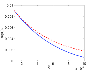
Figure 1: The dependence of m(0,0) on the parameter $\xi$. The cases with and without velocity renormalization are represented by solid and dashed lines, respectively.

In order to investigate the influence of fermion velocity renormalization on the dynamical mass, we now need to calculate the fermion self-energy due to gauge fluctuations. This will be done perturbatively. To the leading order of $1/N$ expansion, the self-energy is

$$\Sigma(p) = \int\frac{d^{3}k}{(2\pi)^{3}}\gamma^{\mu}S_{0}(k)\gamma^{\nu}D_{\mu\nu}(p-k)$$ (16)

$$= \Sigma_{A}(p)+\Sigma_{B}(p),$$

where

$$\Sigma_{A}(p) \equiv \int\frac{d^{3}k}{(2\pi)^{3}}\gamma^{\mu}S_{0}(k)\gamma^{\nu}\frac{A_{\mu\nu}(p-k)}{\Pi_{A}^{f}(p-k)+\xi},$$

$$\Sigma_{B}(p) \equiv \int\frac{d^{3}k}{(2\pi)^{3}}\gamma^{\mu}S_{0}(k)\gamma^{\nu}\frac{B_{\mu\nu}(p-k)}{\Pi_{B}^{f}(p-k)}.$$ (17)

After tedious but straightforward calculations, we found that, the longitudinal contribution is

$$\Sigma_{A}(p) = -\frac{4i}{N\pi^{2}}\gamma^{0}p_{0}\ln\left(\frac{\Lambda}{\max{(p,\xi)}}\right)\approx-\frac{4i}{N\pi^{2}}\gamma^{0}p_{0}\ln\left(\frac{\Lambda}{p+\xi}\right)$$ (18)

$$= -\frac{4i}{N\pi^{2}}\gamma^{0}p_{0}\left[\ln\left(\frac{\Lambda}{p}\right)+\ln\left(\frac{p}{p+\xi}\right)\right],$$

and the transverse contribution is

$$\Sigma_{B}(p)=\frac{4i}{3N\pi^{2}}\gamma^{0}p_{0}\ln\left(\frac{\Lambda}{p}\right)-\frac{8i}{3N\pi^{2}}v\gamma\cdot\mathbf{p}\ln\left(\frac{\Lambda}{p}\right),$$ (19)

with $\Lambda$ the ultraviolet cutoff. Then the total self-energy can be written as

$$\Sigma(p)=\Sigma_{0}(p)i\gamma^{0}p_{0}+\Sigma_{1}(p)iv\mathbf{\gamma}\cdot\mathbf{p},$$ (20)

where

$$\Sigma_{0}(p) = -\frac{8}{3N\pi^{2}}\ln\left(\frac{\Lambda}{p}\right)-\frac{4}{N\pi^{2}}\ln\left(\frac{p}{p+\xi}\right),$$ (21)

$$\Sigma_{1}(p) = -\frac{8}{3N\pi^{2}}\ln\left(\frac{\Lambda}{p}\right).$$ (22)

It is easy to see that, the temporal component of wave function renormalization $\mathcal{A}_{0}(p)$ is equal to $1+\Sigma_{0}(p)$ and the spatial component is $\mathcal{A}_{1}(p)=1+\Sigma_{1}(p)$. In the absence of non-relativistic scalar bosons, QED₃ respects the Lorentz invariance, so $\Sigma_{1}(p)=\Sigma_{0}(p)$. In the present problem, the non-relativistic scalar bosons breaks the Lorentz invariance, so that $\Sigma_{1}(p)\neq\Sigma_{0}(p)$. Indeed, the velocity renormalization is determined by their difference, $\Sigma_{1}(p)-\Sigma_{0}(p)=-\frac{4}{N\pi^{2}}\ln\left(\frac{p+\xi}{p}\right)$. Applying the standard renormalization group (RG) method Shankar94 ; Son07 ; Sachdev08 ; WangJ11 , one can approximately obtain the flow equation for fermion velocity in the low-energy regime,

$$p\frac{\partial v(p)}{\partial p}=\frac{4}{N\pi^{2}}v(p).$$ (23)

Its solution can be formally written as

$$v(p)=\left(\frac{p}{p+\xi}\right)^{\eta},$$ (24)

where $\eta=\frac{4}{N\pi^{2}}$ is the anomalous dimension. It is interesting to notice that for $\xi=0$, $v(p)=1$, so the fermion velocity will not be renormalized when the Lorentz invariance is restored.

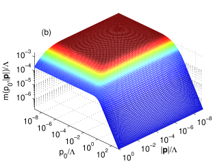
Figure 2: Dynamical mass $m(p_{0},|\mathbf{p}|)$ with (a) for $\xi/\Lambda=10^{-3}$ and (b) for $\xi/\Lambda=10^{-2}$.

In order to consider the influence of fermion velocity renormalization on mass generation, we will replace the bare fermion velocity by its renormalized value. Such approach was recently employed by Khveshchenko to study an analogous issue in the context of graphene Khveshchenko09 . Replacing the bare fermion velocity in Eq.(15) by the renormalized velocity Eq.(24), we now have a new mass equation,

$$m(p_{0},|\mathbf{p}|)=\frac{8}{N}\int\frac{d^{3}k}{(2\pi)^{3}}\frac{m(k_{0},|\mathbf{k}|)}{k_{0}^{2}+v^{2}(k)|\mathbf{k}|^{2}+m^{2}(k_{0},|\mathbf{k}|)}\times\Bigl{[}\frac{1}{\frac{\sqrt{q_{0}^{2}+v^{2}(q)|\mathbf{q}|^{2}}}{v^{2}(q)}+\frac{8}{N}\xi}+\frac{1}{\frac{\sqrt{q_{0}^{2}+v^{2}(q)|\mathbf{q}|^{2}}}{v^{2}(q)}}\Bigl{]},$$ (25)

where $q_{0}=p_{0}-k_{0}$ and $\mathbf{q}=\mathbf{p}-\mathbf{k}$.

In the numerical computation, we fix $N=2$, corresponding to the physical flavor. In Fig.(1), the cases with and without velocity renormalization are represented by solid and dashed lines, respectively. The dynamical mass functions $m(p_{0},|\mathbf{p}|)$ in the presence of velocity renormalization are shown in Fig.(2) with (a) for $\xi/\Lambda=10^{-3}$ and (b) for $\xi/\Lambda=10^{-2}$. From the figures, we can draw two main conclusions. First, DCSB still happens for flavor $N=2$ after taking into account the scalar bosons, and indeed survives when $\xi$ is smaller than a critical value $\xi_{c}$. This indicates that it is not suitable to simply discard the temporal component of gauge field Kim97 ; Kim99 . Second, the fermion velocity renormalization enhances the dynamical fermion mass in the present QED₃ model. This is apparently very different from the behavior of Dirac fermion in long-range Coulomb interactionKhveshchenko09 ; Sabio10 ; Son07 , where the interaction takes the form

$$V_{C}(q_{0},|\mathbf{q}|)=\frac{1}{\frac{|\mathbf{q}|}{2\pi gv}+\frac{N}{8}\frac{|\mathbf{q}|^{2}}{\sqrt{q_{0}^{2}+v^{2}|\mathbf{q}|^{2}}}},$$ (26)

with $g$ the coupling constant of Coulomb interaction. In the limit of infinite Coulomb repulsion $g\to\infty$, it was shown Khveshchenko09 ; Son07 that the renormalized fermion velocity is

$$v(p)=\left(\frac{p}{\Lambda}\right)^{-\eta}.$$ (27)

Evidently, the renormalized fermion velocity is reduced in the low energy regime in our QED₃ model (see Eq.(24)), but becomes larger in the case of Coulomb interaction (see Eq.(27)). This difference leads to the different effects of velocity renormalization on dynamical mass generation in gauge-interacting and Coulomb-interacting systems.

We finally remark on the applications of our results. It is known that the high-T_c superconductor at zero doping is a Mott insulator with long-range AFM order Lee06 . Such long-range order persists at small doping concentration $x$, but is completely destroyed when $x>0.03$ Lee06 . Within the effective gauge theory of high-T_c superconductor, the doping process amounts to introducing non-relativistic scalar boson $\phi$, while the AFM order is represented by DCSB. In Ref. Kim99 , it was argued that AFM order is immediately destroyed once scalar boson is present, which is not well consistent with the experimental facts. Our calculations show that DCSB can occur in the presence of scalar boson as long as parameter $\xi$ is sufficiently small, but is destroyed when $\xi>\xi_{c}$. On general physical grounds, the compressibility parameter $\xi$ should depend on the density of scalar boson (doping). Therefore, our results imply that AFM is destroyed only when doping exceeds certain critical value. This is qualitatively consistent with experimental facts.

We are grateful to Guo-Zhu Liu for his encouragement and supervision. This work was supported by the National Natural Science Foundation of China under Grant No. 11074234, No.11075149 and No.10975128.

References

- (1) Pisarski P 1984 Phys. Rev. D 29 2423
- (2) Appelquist T W et al 1986 Phys. Rev. D 33 3704
- (3) Appelquist T W et al 1988 Phys. Rev. Lett. 60 2575
- (4) Nash D 1989 Phys. Rev. Lett. 62 3024
- (5) Dagotto E et al 1989 Phys. Rev. Lett. 62 1083
- (6) Atkinson D 1990 Phys. Rev. D 42 602
- (7) Pennington M R et al 1991 Phys. Lett. B 253 246
- (8) Appelquist T W et al 1995 Phys. Rev. Lett. 75 2081
- (9) Gusynin V P 1996 Phys. Rev. D 53 2227
- (10) Maris P 1996 Phys. Rev. D 54 4049
- (11) Hands S J et al 2002 Nucl. Phys. B 645 321
- (12) Liu G Z and Cheng G 2002 Phys. Rev. B 66 100505(R)
- (13) Liu G Z and Cheng G 2003 Phys. Rev. D 67 065010
- (14) Fischer C S et al 2004 Phys. Rev. D 70 073007
-
(15)
Feng H T et al 2006 Phys. Rev. D 73 016004;
Feng H T et al 2008 Phys. Lett. B 661 57;
Feng H T et al 2010 Phys. Lett. B 688 178 - (16) Hu F et al 2008 Chin. Phys. Lett. 25 2823
- (17) Jiang H et al 2008 J. Phys. A: Math. Theor. 41 255402
- (18) Liu G Z et al 2010 Nucl. Phys. B 825 303
- (19) Li W and Liu G Z 2010 Phys. Rev. D 81 045006
- (20) Zhou Y Q and Yang Y H 2011 Chin. Phys. Lett. 28 041101
- (21) Burden C J et al 1992 Phys. Rev. D 46 2695
- (22) Maris P 1995 Phys. Rev. D 52 6087
- (23) Wang J et al 2010 Phys. Rev. D 82 067701
- (24) Affleck I and Marston J B 1988 Phys. Rev. B 37 3774
- (25) Ioffe L B and Larkin A I 1989 Phys. Rev. B 39 8988
- (26) Dorey N et al 1992 Nucl. Phys. B 386 614
-
(27)
Wen X G and Lee P A 1996 Phys. Rev. Lett. 76 503;
Lee P A et al 1998 Phys. Rev. B 57 6003 - (28) Kim D H et al 1997 Phys. Rev. Lett. 79 2109
- (29) Kim D H and Lee P A 1999 Ann. Phys. (N.Y.) 272 130
- (30) Rantner W and Wen X G 2001 Phys. Rev. Lett. 86 3871
-
(31)
Franz M and Tešanović Z 2001 Phys. Rev. Lett. 87 257003
Herbut I F 2002 Phys. Rev. B 66 100505 - (32) Hermele M et al 2004 Phys. Rev. B 70 214437
- (33) Lee P A et al 2006 Rev. Mod. Phys. 78 17
- (34) Wang J R and Liu G Z 2010 Nucl. Phys. B 832 441
- (35) Wang J R and Liu G Z 2010 Phys. Rev. B 82 075133
- (36) Wang J et al 2011 Phys. Rev. B 83 214503
- (37) Zhang S C et al 1989 Phys. Rev. Lett. 62 82
- (38) Halperin B I et al 1993 Phys. Rev. B 47 7312
- (39) Wang J and Liu G Z 2012 in preparation
- (40) Khveshchenko D V 2009 J. Phys.: Condens. Matter 21 075303
- (41) Sabio J et al 2010 Phys. Rev. B 82 121413(R)
- (42) Shankar R 1994 Rev. Mod. Phys. 66 129
- (43) Son D T 2007 Phys. Rev. B 75 235423
- (44) Huh Y and Sachdev S 2008 Phys. Rev. B 78 064512