Properties of design-based estimation under stratified spatial sampling with application to canopy coverage estimation

Abstract

The estimation of the total of an attribute defined over a continuous planar domain is required in many applied settings, such as the estimation of canopy coverage in the Monterano Nature Reserve in Italy. If the design-based approach is considered, the scheme for the placement of the sample sites over the domain is fundamental in order to implement the survey. In real situations, a commonly adopted scheme is based on partitioning the domain into suitable strata, in such a way that a single sample site is uniformly placed (i.e., selected with uniform probability density) in each stratum and sample sites are independently located. Under mild conditions on the function representing the target attribute, it is shown that this scheme gives rise to an unbiased spatial total estimator which is “superefficient” with respect to the estimator based on the uniform placement of independent sample sites over the domain. In addition, the large-sample normality of the estimator is proven and variance estimation issues are discussed.

, and

1 Introduction

Applied scientists frequently deal with attributes defined on continuous spatial domains. In this framework, if the design-based approach is assumed, the target attribute may be expressed as a fixed bounded function $y$ taking values on the study region $A$ (a suitable subset of the plane). In the simplest case, $y(u)$ may represent the value of the attribute at $u\in A$. As an example, in an environmental survey, $y(u)$ could be the air-borne pollutant level at the sample site $u$ on a landscape. In a more structured setting, $y(u)$ may also describe the “attribute density” arising from the selected spatial sampling design [this topic is extensively considered and explained in Chapter 10 of Gregoire and Valentine (2008)]. As an example, by supposing a fixed-radius circular plot sampling in a forest survey, $y(u)$ could represent the number of trees lying in the plot centered at the sample site $u$ [up to a known proportionality constant; see Gregoire and Valentine (2008), pages 328–332]. In this case, under the design-based approach, the population universe is constituted by a continuum (ideally by the noncountable set of sample sites on $A$) and the inference is actually carried out by assuming the so-called “continuous-population” paradigm. This approach has been extensively considered in recent years on the basis of the seminal papers by de Gruijter and ter Braak (1990), Cordy (1993) and Brus and de Gruijter (1997).

In the described framework, the estimation goal is usually focused on the spatial total, that is,

$$T=\int_{A}y(u)\,\mathrm{d}u$$ (1)

[see, e.g., Stevens (1997) and Chapter 10 of Gregoire and Valentine (2008)]. Indeed, as emphasized by Stevens (1997), the integral representation in (1) embraces a general family of population parameters, such as means, proportions or distribution functions. In order to estimate $T$, the key problem of the design-based approach is the selection of an appropriate sampling strategy. As usual, it is assumed that the sampling strategy includes the joint selection of a suitable estimator and the corresponding scheme for the placement of the $n$ sample sites on the study region $A$. Since an integral representation for $T$ holds, it is quite evident that the estimation problem may be rephrased in terms of the Monte Carlo integration theory. Interestingly, known Monte Carlo integration strategies are equivalent to the sampling strategies which are commonly adopted in environmental and ecological studies [Barabesi (2003, 2007), Gregoire and Valentine (2008), page 327]. Similar Monte Carlo integration approaches to parameter estimation occur in very different research areas, such as in stereology [see, e.g., the monograph by Baddeley and Jensen (2005)] or in computer graphics [see, e.g., Agarwal et al. (2003)].

The basic reference sampling scheme for selecting the sample sites is the Uniform Random Sampling (URS), which constitutes the continuous-population analog to simple random sampling from a finite population [Cordy (1993)]. Under URS, the $n$ sample sites are independently and uniformly selected on $A$ [Figure 1(a)]. Despite its simplicity, URS may be not suitable in practice since it may produce an uneven coverage of the study region and the corresponding unbiased estimator of $T$ displays a variance of order $n^{-1}$, that is, the variance decreases to $0$ at the rate $n^{-1}$ as $n\rightarrow\infty$. In any case, URS is often considered a helpful benchmark to compare the performance of more refined schemes.

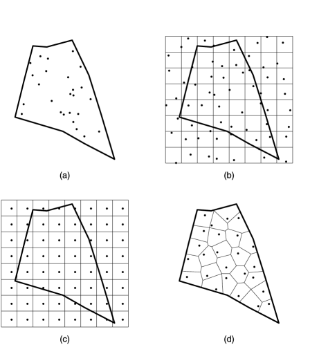
Figure 1: Placement of $n=25$ sample sites over a study region $A$ according to the URS scheme (a), the TSS scheme (b), the SGS scheme (c) and the SS scheme based on equal-size strata obtained by means of the Brus, Spätjens and de Gruijter (1999) algorithm (d). For the TSS and SGS schemes, the set $R$ is chosen as a rectangle and the tessellation is based on squares, while $n$ represents the mean number of sample sites in $A$.

In order to overcome the drawbacks involved with URS, a sampling scheme frequently adopted in environmental studies is the so-called Tessellation Stratified Sampling (TSS) [see, e.g., Stevens (1997) and the U.S. Environmental Protection Agency (2002), page 63]. The TSS scheme is initially implemented by superimposing a suitable set $R$ onto the study region in such a way that $A\subseteq R$ and by introducing the analytical extension $y_{e}$ of $y$ on $R$. Formally, the analytical extension is defined as $y_{e}(u)=y(u)$ if $u\in A$ and $y_{e}(u)=0$ if $u\in R\setminus A$. Obviously, in this setting (1) may be conveniently rewritten as $T=\int_{R}y_{e}(u)\,\mathrm{d}u$. Subsequently, a regular tessellation of $R$ is carried out and one sample site is independently and uniformly selected in each tessellation element [Figure 1(b)]. The theoretical properties of the TSS scheme have been explained in detail [Barabesi and Marcheselli (2003, 2005a, 2005b, 2008)]. The scheme gives rise to an unbiased estimator for $T$ with variance of order $n^{-\gamma}$, where $\gamma\in(1,2]$. Hence, the estimator under TSS is “superefficient” since its variance decreases to $0$ faster than the variance of the estimator under URS as $n\rightarrow\infty$. The parameter $\gamma$ depends on the degree of regularity of the analytical extension $y_{e}$: for instance, it turns out that $\gamma=2$ for smooth functions, but it can occur that $\gamma=3/2$ even for noncontinuous and rather irregular functions [Barabesi and Marcheselli (2003, 2005a, 2008)]. Hence, the variance of the estimator for $T$ decreases to $0$ faster as $y_{e}$ becomes more regular. In addition, consistent variance estimation is available if $y_{e}$ is a differentiable function on $R$ [Barabesi and Marcheselli (2003, 2008)]. In order to avoid the difficulties involved in the variance estimation, Cordy and Thompson (1995) and Stevens (1997) suggest modifying the TSS scheme by randomly shifting the tessellation. The randomized TSS scheme does not involve extra-sampling effort and allows for unbiased variance estimation without any restriction on the function $y_{e}$ [Stevens (1997)], even if the consistency of the variance estimator has not been proved. Barabesi and Franceschi (2011) show that the TSS scheme and its randomized modification produce estimators for $T$ with identical variance convergence rates.

A further frequently-considered scheme is Systematic Grid Sampling(SGS), which constitutes a systematic version of the TSS scheme [see, e.g., Valentine, Affleck and Gregoire (2009) and the U.S. Environmental Protection Agency (2002), page 70]. The SGS scheme provides the continuous-population analog to systematic sampling from a finite population as considered by Madow and Madow (1944) [see also D’Orazio (2003), as to systematic sampling of a spatial finite population]. Similarly to TSS, the SGS scheme requires a regular tessellation of $R$ and the extension of the function $y$ on $R$. However, under SGS, a sample site is uniformly generated in the reference tessellation element and it is systematically repeated in the other tessellation elements [see Figure 1(c)]. The SGS scheme is commonly adopted in stereology and gives rise to an unbiased “superefficient” estimator for $T$, under certain smoothness conditions on $y_{e}$ [Cruz-Orive (1993), Baddeley and Jensen (2005), page 159]. However, the variance of the estimator tends to be extremely elevated when the periodicity in the function $y_{e}$ is “in phase” with the tessellation elements [Baddeley and Jensen (2005), Chapter 13].

Even if the TSS and SGS schemes allow for an even coverage of the study region and give rise to unbiased “superefficient” estimation for $T$, these schemes suffer due to two main technical drawbacks which are related to the analytical extension of $y$ on $R$. Indeed, the sample sites are actually placed on $R$ (not on $A$) and, hence, the number of sample sites on $A$ is a random variable, unless $A$ is exactly tessellated. Obviously, the tessellation may be selected in such a way that the mean number of sample sites on $A$ equals the prefixed sample size $n$ [as an example, this procedure is adopted for Figure 1(b) and (c)]. However, the task is generally undesirable for field scientists, who usually require reproducible designs. Moreover, even if the function $y$ is regular on $A$, the function $y_{e}$ is likely to be not continuous on the boundary of $A$ (and hence on $R$), unless $y$ is null on this boundary. As previously explained, the lack of regularity considerably reduces the efficiency of the estimators for $T$.

An alternative way to face the whole setting may be based on stratification methods involving the “one-per-stratum” placement of the sample sites. More precisely, under the “one-per-stratum” Stratified Sampling (SS), the study region $A$ is partitioned into $n$ suitable strata and one sample site is independently and uniformly selected in each stratum [Figure 1(d)]. The scheme constitutes the continuous-population counterpart to the classic “one-per-stratum” stratified sampling in the finite-population setting [see, e.g., Cochran (1946)]. Moreover, the SS scheme generalizes the TSS scheme when $A$ coincides with $R$ and the tessellation is noncongruent. The scheme is commonly adopted for environmental and agricultural surveys [see, e.g., Walvoort, Brus and de Gruiter (2010) and the references therein].

In this paper, it is proven that the SS scheme produces an unbiased “superefficient” estimator for $T$, which shares the variance properties of the estimator under the TSS scheme. However, in contrast with the TSS and SGS schemes, when the SS scheme is adopted the $n$ sample sites are exactly placed on $A$ and no analytical extension of $y$ is introduced. Moreover, in real surveys spatial stratification is often demanded in practice, owing to geographical or administrative convenience and tessellation-based methods would not be applicable. In addition, there exist ad hoc algorithms for partitioning the study region into strata (eventually of the same size) with suitable geometrical and statistical properties [Brus, Spätjens and de Gruijter (1999), Walvoort, Brus and de Gruiter (2010)]. Finally, even if schemes with more than a single sample site per stratum may be considered, it is apparent that the benefits arising from the full force of the stratification are achieved by adopting the “one-per-stratum” allocation. In any case, the “two-per-stratum” scheme will be briefly considered since it produces unbiased and consistent variance estimation.

Even if the achieved results may be applied to a broad range of different data sets collected on a continuous spatial domain, the motivating practical setting of the paper originates from an experiment dealing with canopy coverage estimation in the Monterano Nature Reserve. Owing to the complex boundary mosaic of this forest, the estimation approach based on forest polygon delineation and area mensuration in the GIS environment may produce omission and commission errors (which tend to be systematic) in the image interpretation. In order to overcome these shortcomings, a survey procedure based on line-intercept sampling which just involves the measurement of the intersections of linear transects with forest patches is considered. As to the Monterano Nature Reserve, forest researchers collected data by placing transect midpoints according to the SS scheme with equal-size strata by means of the Brus, Spätjens and de Gruijter (1999). Hence, the results of this paper may be suitably applied in order to provide point and interval estimation of canopy coverage.

2 Spatial total estimation

As pointed out in the Introduction, the benchmark for comparing different schemes is the URS and, hence, spatial total estimation under this scheme is briefly described. If $U_{1},U_{2},\ldots,U_{n}$ are $n$ i.i.d. random variables representing the sample-site locations, in such a way that each $U_{i}$ is uniformly distributed on $A$, the usual unbiased estimator for $T$ under URS [see, e.g., Cordy (1993)] is

$$\widetilde{T}_{n}=\frac{a(A)}{n}\sum_{i=1}^{n}y(U_{i}),$$ (2)

where $a(\cdot)$ denotes the area of a set in $\mathbb{R}^{2}$ (technically, $a$ represents the Lebesgue measure in $\mathbb{R}^{2}$). The variance of the estimator in (2) is given by

$$\operatorname{Var}[\widetilde{T}_{n}]=\frac{1}{n}\bigl{(}a(A)S-T^{2}\bigr{)},$$

where $S=\int_{A}y(u)^{2}\,\mathrm{d}u$, and, hence, it turns out that $\operatorname{Var}[\widetilde{T}_{n}]=O(n^{-1})$. As usual, if $\{a_{n}\}$ and $\{b_{n}\}$ represent two positive sequences, $a_{n}=O(b_{n})$ means that the ratio $a_{n}/b_{n}$ is bounded for all $n$.

Under the SS scheme, the study region $A$ is partitioned in $n$ strata $A_{1},\allowbreak A_{2},\ldots,A_{n}$, in such a way that each stratum is connected and compact (in a topological sense), and one sample-site location is independently and uniformly selected in each stratum. Therefore, let us suppose that the sample-site locations are represented by the random variables $V_{1},V_{2},\ldots,V_{n}$. According to the continuous Horvitz–Thompson Theorem [Cordy (1993)], an unbiased estimator for (1) under SS is

$$\widehat{T}_{n}=\sum_{i=1}^{n}a(A_{i})y(V_{i})$$ (3)

with variance

$$\sigma_{n}^{2}=\operatorname{Var}[\widehat{T}_{n}]=\sum_{i=1}^{n}a(A_{i})^{2}\operatorname{Var}[y(V_{i})]=\sum_{i=1}^{n}a(A_{i})S_{i}-\sum_{i=1}^{n}T_{i}^{2},$$

where $T_{i}=\int_{A_{i}}y(u)\,\mathrm{d}u$ and $S_{i}=\int_{A_{i}}y(u)^{2}\,\mathrm{d}u$.

In order to assess the variance properties of the estimator in (3), let us assume that $y$ is a Hölder function on $A$, that is, a function satisfying the condition

$$|y(u)-y(v)|\leq H\|u-v\|^{\alpha},$$

where $H<\infty$, $\alpha\in(0,1]$ and $u,v\in A$, while $\|\cdot\|$ denotes the usual norm in $\mathbb{R}^{2}$, that is, $\|u-v\|$ denotes the distance between the points $u$ and $v$. Obviously, $y$ reduces to a Lipschitz function for the special case $\alpha=1$. The family of Hölder functions is very large [for more details, see, e.g., Evans (2010), page 254]. Indeed, it is at once apparent that Hölder functions are continuous. In addition, from the above definition, it also follows that the family of Hölder functions contains the family of Lipschitz functions, which in turn contains the family of continuously differentiable functions. Informally speaking, the Hölder condition quantifies the local variation of the function $y$, in such a way that the index $\alpha$ may be interpreted as the corresponding “degree of local continuity.” Hence, the family of Hölder functions encompasses “smooth” functions, as well as functions displaying a very irregular behavior. As a matter of fact, there exist Hölder functions which are continuous, but nowhere differentiable.

By assuming that

$$\operatorname{diam}(B)={\sup_{u,v\in B}}\|u-v\|$$

represents the diameter of a given set $B$, that is, the largest distance between two points in $B$, let

$$d_{n}=\max_{i=1,2,\ldots,n}\operatorname{diam}(A_{i})$$

be the maximum diameter of the $A_{i}$’s. Hence, let us consider the condition

$$d_{n}^{2}\leq bn^{-1},$$ (4)

where $b>0$ is a bounded constant. Since

$$a(A_{i})\leq\operatorname{diam}(A_{i})^{2}\leq d^{2}_{n},\qquad i=1,2,\ldots,n,$$

condition (4) implies that

$$a(A_{i})\leq bn^{-1},\qquad i=1,2,\ldots,n.$$

In addition, let us also consider the condition

$$a(A_{i})\geq cn^{-1},\qquad i=1,2,\ldots,n,$$ (5)

where $c>0$ is a bounded constant. It should be remarked that condition (4) simply requires that the stratification be performed by assuming quite “homogeneous” strata, that is, avoiding strata having “stretched” shapes and in such a way that no “large” strata are admitted as $n\rightarrow\infty$. In addition, condition (5) actually ensures that too “small” strata are in turn avoided as $n\rightarrow\infty$. These requirements are likely to hold for practical choices of $A_{1},A_{2},\ldots,A_{n}$. Obviously, condition (5) is always satisfied with equal-size strata, that is, when $a(A_{i})=a(A)/n$ for $i=1,2,\ldots,n$.

On the basis of Result 1 in the Appendix, by assuming that $y$ is a Hölder function and that condition (4) holds, it turns out that

$$\sigma_{n}^{2}=O(n^{-1-\alpha}).$$

Hence, the SS scheme may lead to a noticeable estimation improvement with respect to the basic URS scheme. The best variance order $n^{-2}$ is achieved when $y$ is a Lipschitz function. In any case, the SS scheme produces more efficient estimation with respect to URS for each $\alpha$ value as $n\rightarrow\infty$. The gain may be remarkable since in many real surveys $\alpha$ is likely to be about one—for example, as to the canopy coverage estimation considered in Section 4; see the discussion after the formula in (11).

The achieved variance properties may be extended to a larger class of functions. More precisely, let $y$ be a piecewise Hölder function on $A$, that is, there exists a finite partition of $A$ in such a way that $y$ is a Hölder function on each partition element and the partition boundary is rectifiable, that is, in practical terms the boundary is “smooth.” This setting is of real interest, since $y$ often belongs to this function family when $y$ represents the “attribute density” as defined in the Introduction. Thus, by assuming that $y$ is a piecewise Hölder function and that condition (4) holds, on the basis of Result 2 in the Appendix, it turns out that

$$\sigma_{n}^{2}=O\bigl{(}n^{-\min(1+\alpha,3/2)}\bigr{)}.$$

Hence, even if the gain is lessened owing to the discontinuity of the function $y$, the performance of the SS scheme is in turn considerable. In this case, the best variance order $n^{-3/2}$ is achieved when $y$ is a piecewise Hölder function with $\alpha\geq 1/2$. In turn, the SS scheme is preferable with respect to the URS scheme for each $\alpha$.

As to the large-sample normality of the estimator in (3), on the basis of Result 3 in the Appendix, by assuming that $y$ is a Hölder function and that conditions in (4) and in (5) hold, it follows that

$$\frac{\widehat{T}_{n}-T}{\sigma_{n}}\stackrel{{\scriptstyle\mathcal{L}}}{{\longrightarrow}}N(0,1)$$

as $n\rightarrow\infty$. This convergence result holds even if $y$ is a piecewise Hölder function (see Remark 2 in the Appendix). These findings on the variance properties and the large-sample normality of the estimator in (3) are in complete agreement with the results obtained by Barabesi and Marcheselli (2003, 2005a, 2008) and Barabesi and Franceschi (2011) under TSS. Indeed, the TSS scheme may be considered a special case of the SS scheme when $A$ coincides with $R$ and the strata correspond to the elements of the tessellation.

It should be finally emphasized that for each $n$ the variance of the estimator under URS is greater than or equal to the variance of the estimator under SS when the strata are of the same size, that is, it holds that

$$\operatorname{Var}[\widetilde{T}_{n}]\geq\operatorname{Var}[\widehat{T}_{n}].$$

Indeed, in this case the previous inequality is verified since $T=\sum_{i=1}^{n}T_{i}$ and $S=\sum_{i=1}^{n}S_{i}$, while the inequality

$$\sum_{i=1}^{n}T_{i}^{2}\geq\frac{1}{n}\Biggl{(}\sum_{i=1}^{n}T_{i}\Biggr{)}^{2}$$

obviously holds.

3 Variance estimation

The estimation of $\sigma_{n}^{2}$ is not a trivial task, since a single observation per stratum is available and the strata generally do not constitute a regular tessellation, that is, the strata display different sizes and shapes. In such a setting, estimators relying on contrast-based techniques—such as the proposals by Barabesi and Marcheselli (2003, 2008) under TSS or the proposal by Stevens and Olsen (2003) under randomized TSS—seem quite difficult to implement. However, a simple estimator may be obtained by treating the sample as if it were obtained under the URS scheme. A similar procedure is suggested by Stevens and Olsen (2003) under the randomized TSS scheme. Hence, a naïve estimator for $\sigma_{n}^{2}$ is given by

$$\widehat{\sigma}_{n}^{2}=\frac{n}{n-1}\sum_{i=1}^{n}\biggl{(}a(A_{i})y(V_{i})-\frac{\widehat{T}_{n}}{n}\biggr{)}^{2}.$$ (6)

Since

$$\mathrm{E}[\widehat{\sigma}_{n}^{2}]=\sigma_{n}^{2}+\mathrm{B}[\widehat{\sigma}_{n}^{2}],$$

where

$$\mathrm{B}[\widehat{\sigma}_{n}^{2}]=\frac{n}{n-1}\sum_{i=1}^{n}\biggl{(}T_{i}-\frac{T}{n}\biggr{)}^{2}$$

(Result 4 in the Appendix), the estimator in (6) is positively biased. Moreover, if $y$ is a Hölder function and condition (4) holds, it follows that

$$\mathrm{B}[\widehat{\sigma}_{n}^{2}]=O(n^{-1})$$

(Result 4 in the Appendix). Hence, even if B$[\widehat{\sigma}_{n}^{2}]$ vanishes for large $n$, it might be of a larger order than that of $\sigma_{n}^{2}$. Moreover, if condition (5) holds, on the basis of Remark 1 in the Appendix, it promptly turns out that

$$\frac{\mathrm{B}[\widehat{\sigma}_{n}^{2}]}{\sigma_{n}^{2}}=O(n).$$

In any case, the behavior of this type of estimator seems quite stable in practice as emphasized by Stevens and Olsen (2003), even if its use may lead to a marked overestimation of $\sigma_{n}^{2}$.

For equal-size strata, an alternative estimator displaying more appealing features may be proposed. The suggested estimator is given by

$$\widetilde{\sigma}_{n}^{2}=\frac{a(A)^{2}}{2n^{2}}\Biggl{(}y(V_{1})^{2}+\sum_{i=1}^{n-1}\bigl{(}y(V_{i})-y(V_{i+1})\bigr{)}^{2}+y(V_{n})^{2}\Biggr{)}.$$ (7)

Since

$$\mathrm{E}[\widetilde{\sigma}_{n}^{2}]=\sigma_{n}^{2}+\mathrm{B}[\widetilde{\sigma}_{n}^{2}],$$

where

$$\mathrm{B}[\widetilde{\sigma}_{n}^{2}]=\frac{1}{2}\Biggl{(}T_{1}^{2}+\sum_{i=1}^{n-1}(T_{i}-T_{i+1})^{2}+T_{n}^{2}\Biggr{)}$$

(Result 5 in the Appendix), the estimator in (7) is positively biased. By assuming that

$$D_{n}={\max_{i=1,2,\ldots,n-1}\sup_{u\in A_{i},v\in A_{i+1}}}\|u-v\|,$$

let us consider the condition

$$D_{n}^{2}\leq kn^{-1}$$ (8)

with $k>0$ a suitable bounded constant. Condition (8) actually requires that the stratification be performed by indexing the strata in such a way that $A_{i}$ and $A_{i+1}$ not be “too far” with respect to each other. In practical situations, $A_{i}$ and $A_{i+1}$ may be generally chosen as “neighbors,” that is, in such a way that they share part of their boundary. For example, in the case study contained in Section 4, the partition elements are equally-sized strata which are indexed in such a way that the $i$th and the $(i+1)$th strata have a side in common (see Figure 2). If $y$ is a Hölder function and conditions (4) and (8) are satisfied, it follows that

$$\mathrm{B}[\widetilde{\sigma}_{n}^{2}]=O(n^{-1-\alpha})$$

and

$$\limsup_{n}\biggl{|}\frac{\widetilde{\sigma}_{n}^{2}-\mathrm{E}[\widetilde{\sigma}_{n}^{2}]}{\sigma_{n}^{2}}\biggr{|}=0$$

(Result 5 in the Appendix). Hence, the bias order of the estimator in (7) is reduced with respect to the estimator in (6) and B$[\widetilde{\sigma}_{n}^{2}]$ is of the same order as that of $\sigma_{n}^{2}$. Moreover, if condition (5) holds, and on the basis of Remark 1 in the Appendix, it follows that

$$\frac{\mathrm{B}[\widetilde{\sigma}_{n}^{2}]}{\sigma_{n}^{2}}=O(n^{1-\alpha}).$$

Hence, when $y$ is a Lipschitz function, it turns out that

$$0\leq\frac{\mathrm{B}[\widetilde{\sigma}_{n}^{2}]}{\sigma_{n}^{2}}\leq m,$$

where $m>0$ is a suitable bounded constant, while

$$1\leq\liminf_{n}\frac{\widetilde{\sigma}_{n}^{2}}{\sigma_{n}^{2}}\leq\limsup_{n}\frac{\widetilde{\sigma}_{n}^{2}}{\sigma_{n}^{2}}\leq 1+m$$

(Result 5 in the Appendix), that is, the estimator in (7) is large-sample conservative.

Figure 2: The Monterano Nature Reserve and the corresponding partition in $n=50$ strata according to the SS scheme based on equal-size strata obtained by means of the Brus, Spätjens and de Gruijter (1999) algorithm.

Finally, unbiased and consistent variance estimation is achieved if two sample sites are placed in each stratum, that is, if the “two-per-stratum” SS scheme is actually adopted. In this case, let us assume that $n$ is even and that a partition of the study region into $n/2$ strata is carried out. Obviously, $n$ is now required to be even for comparison purposes with respect to the “one-per-stratum” SS scheme. Moreover, let $V_{1,j}$ and $V_{2,j}$ represent the two sample sites uniformly and independently selected onto the $j$th stratum ($j=1,2,\ldots,n/2$). An unbiased estimator for $T$ is given by

$$\widehat{T}_{2,n}=\frac{1}{2}\sum_{j=1}^{n/2}a(A_{j})\bigl{(}y(V_{1,j})+y(V_{2,j})\bigr{)},$$ (9)

while its variance is

$$\sigma_{2,n}^{2}=\operatorname{Var}[\widehat{T}_{2,n}]=\frac{1}{2}\sum_{j=1}^{n/2}a(A_{j})^{2}\operatorname{Var}[y(V_{1,j})]=\frac{\sigma_{n/2}^{2}}{2}.$$

Hence, an unbiased and consistent estimator for $\sigma_{2,n}^{2}$ is

$$\widehat{\sigma}_{2,n}^{2}=\frac{1}{4}\sum_{j=1}^{n/2}a(A_{j})^{2}\bigl{(}y(V_{1,j})-y(V_{2,j})\bigr{)}^{2}.$$ (10)

Moreover, by considering Result 1 in the Appendix, when condition (4) holds it turns out that

$$\sigma_{2,n}^{2}=O(n^{-1-\alpha})$$

if $y$ is a Hölder function on $A$, while

$$\sigma_{2,n}^{2}=O\bigl{(}n^{-\min(1+\alpha,3/2)}\bigr{)},$$

if $y$ is a piecewise Hölder function on $A$. However, even if the “two-per-stratum” SS scheme provides in turn an unbiased “superefficient” estimator for $T$, it is at once apparent that an efficiency loss occurs in using a stratification based on $n/2$ strata rather than $n$ strata. In addition, if the $n/2$ strata are split in such a way that each stratum is partitioned into two substrata of equal sizes and $\widehat{T}_{n}$ is computed on the basis of this stratification, it is promptly shown that $\operatorname{Var}[\widehat{T}_{2,n}]\geq\operatorname{Var}[\widehat{T}_{n}]$ on the basis of the discussion at the end of Section 2.

4 An application to canopy coverage estimation

In order to illustrate an application of the SS scheme in an environmental survey, the estimation of the canopy coverage in the Monterano Nature Reserve has been considered. The Monterano Nature Reserve (which constitutes the study region $A$ in this case) is located in the central part of Italy (Lazio region) and its geographical boundary is depicted in Figure 2. The area of the Monterano Nature Reserve is equal to $a(A)=1\mbox{,}045$ ha.

If $C\subset A$ represents the region inside $A$ covered by vegetation, canopy coverage is simply defined as the area of $C$, that is, in this case $T=a(C)$. Canopy coverage constitutes a central indicator in forestry, as emphasized by Bonham (1989). In order to estimate this quantity, replicated line-intercept sampling is commonly adopted [Barabesi (2007), Barabesi and Marcheselli (2008)]. More precisely, the replicated line-intercept sampling protocol is carried out by selecting $n$ sample sites on $A$ and by considering $n$ linear transects of fixed length $L$ with the same orientation, in such a way that the transect midpoints are centered on each sample site. According to Barabesi and Marcheselli (2008), the canopy coverage $T$ may be expressed as the integral of the “attribute density,” that is,

$$T=a(C)=\frac{1}{L}\int_{A}l\bigl{(}C\cap t(u)\bigr{)}\,\mathrm{d}u,$$

where $t(u)$ represents the set of points in a transect with midpoint centered at the sample site $u$, while $l(\cdot)$ denotes the length of a set in $\mathbb{R}$ (technically, $l$ represents the Lebesgue measure in $\mathbb{R}$). In this case, it follows that

$$y(u)=\frac{1}{L}l\bigl{(}C\cap t(u)\bigr{)}$$

is the length of the intersection of $t(u)$ with $C$, up to a known constant. Hence, if the SS scheme with equal-size strata is adopted, the canopy coverage estimator reduces to

$$\widehat{T}_{n}=\frac{a(A)}{Ln}\sum_{i=1}^{n}l\bigl{(}C\cap t(V_{i})\bigr{)},$$ (11)

that is, the estimator in (11) actually represents the total sum of the intersection lengths between $C$ and the $n$ transects, up to a known constant. Barabesi and Marcheselli (2008) remark that if the boundary of $C$ is rectifiable, $y$ is a Hölder function. Hence, if condition (4) holds, it turns out that $\operatorname{Var}[\widehat{T}_{n}]=O(n^{-1-\alpha})$. In particular, if $C$ is given by the union of circles or ellipses, it may be proven that $\operatorname{Var}[\widehat{T}_{n}]=O(n^{-2+\varepsilon})$ where $\varepsilon>0$. Moreover, if $C$ is given by the union of polygons, it may be proven that $\operatorname{Var}[\widehat{T}_{n}]=O(n^{-2})$. Hence, in real settings, the estimator in (11) may be very efficient.

Even if the canopy coverage could be estimated by means of polygon delineation on the basis of visual interpretation of remotely sensed imagery, the procedure may typically produce errors and omissions [see, e.g., Corona, Chirici and Travaglini (2004)]. So, in order to avoid the interpretation drawbacks in the estimation of forest features such as forest ecotone or canopy coverage, Corona, Chirici and Travaglini (2004) suggest adopting replicated line-intercept sampling. Hence, for estimating canopy coverage in the Monterano Nature Reserve, the replicated line-intercept sampling protocol has been implemented by assuming the described procedure with $n=50$ transects with fixed direction and length $L=200$ m [these choices are consistent with the study by Corona, Chirici and Travaglini (2004)]. The transect midpoints (displayed in Figure 2) have been placed by adopting the SS scheme with equal-size strata obtained by using the Brus, Spätjens and de Gruijter (1999) algorithm. In this case, the estimator in (11) has given rise to the estimate $660$ ha for the canopy coverage. Hence, $63.16$% of the Monterano Nature Reserve is covered by vegetation. In addition, variance estimation has been performed on the basis of (7) by adopting a sequential indexing of strata with a common side (see Figure 2). Accordingly, the standard deviation estimate is $58$ ha and a conservative confidence interval for canopy coverage at the approximate $95$% confidence level is $(647\mbox{ ha},674\mbox{ ha})$. Thus, a conservative confidence interval at the same level for the percent coverage is given by $(61.87\%,64.46\%)$.

5 Concluding remarks

Under the design-based approach, the target attribute of many surveys can be conceptualized as a suitable fixed function $y$ defined on a given planar domain. This approach is usually described as the continuous-population paradigm and it is especially suitable in environmental and ecological frameworks [see, e.g., Williams and Eriksson (2002) and Gregoire and Valentine (2008), page 2]. Indeed, in such spatial contexts, it is not often possible to achieve an area frame in order to apply the usual finite-population sampling theory. Regrettably, practitioners frequently force the continuous-population setting into the finite-population setting, owing to the lack of results or to the misunderstanding of the continuous-population paradigm.

The continuous-population paradigm requires implementation of an effective probability sampling design to estimate the target parameter, usually the total of the study attribute given by the integral of the function $y$. Hence, a key decision is the choice of the sampling scheme for the placement of sample sites. Schemes based on tessellation and stratification are widely used in natural resource assessment and for environmental monitoring, since evenly-spread sample sites over the study region often simplify collection of field data and estimation efficiency is usually increased. However, as emphasized by Walvoort, Brus and de Gruiter (2010), schemes based on tessellation methods may involve several drawbacks and, hence, stratification schemes may often be preferable.

In the present paper it is shown that the “one-per-stratum” placement of the sample sites produces an unbiased “superefficient” spatial total estimator with respect to the uniform placement of independent sample sites. Variance properties and convergence results for the suggested estimator are given in a purely design-based approach without assuming any super-population model on the spatial correlation structure of the target attribute, as usually considered for systematic and stratified sampling of a two-dimensional population [see, e.g., Bellhouse (1977) and Breidt (1995)]. In contrast, the present findings are achieved by assuming very mild conditions on the function $y$ (which are likely to be met in any real survey) and by requiring simple conditions which avoid strata of too small or too large sizes, as well as strata with stretched shapes.

Appendix

Result 1.

Let $y$ be a Hölder function. Hence, since each $A_{i}$ is assumed to be connected and $y$ is a continuous function, there exists $\bar{u}_{i}\in A_{i}$ for each $i=1,2,\ldots,n$ such that

$$y(\bar{u}_{i})=\mathrm{E}[y(V_{i})].$$

Accordingly, since the Hölder condition holds for $y$, we obtain

$$\operatorname{Var}[y(V_{i})] = \mathrm{E}\bigl{[}\bigl{(}y(V_{i})-\mathrm{E}[y(V_{i})]\bigr{)}^{2}\bigr{]}=\mathrm{E}\bigl{[}\bigl{(}y(V_{i})-y(\bar{u}_{i})\bigr{)}^{2}\bigr{]}$$

$$\leq H^{2}\mathrm{E}[\|V_{i}-\bar{u}_{i}\|^{2\alpha}]$$

$$\leq H^{2}\operatorname{diam}(A_{i})^{2\alpha}\leq H^{2}d^{2\alpha}_{n}.$$

Hence, it holds that

$$\sigma_{n}^{2}=\sum_{i=1}^{n}a(A_{i})^{2}\operatorname{Var}[y(V_{i})]\leq H^{2}d_{n}^{2\alpha}\sum_{i=1}^{n}a(A_{i})^{2}.$$

Since $a(A_{i})\leq d^{2}_{n}$ and $\sum_{i=1}^{n}a(A_{i})=a(A)$, it also turns out that

$$\sigma_{n}^{2}\leq H^{2}d_{n}^{2+2\alpha}a(A).$$

In addition, if condition (4) holds, it follows that

$$\sigma_{n}^{2}\leq b^{1+\alpha}H^{2}a(A)n^{-1-\alpha},$$

that is, $\sigma_{n}^{2}=O(n^{-1-\alpha})$.

Result 2.

Let $y$ be a piecewise Hölder function on $A$. Moreover, by denoting $B$ as the boundary of the partition, let us assume that

$$I=\{i\dvtx A_{i}\cap B\neq\varnothing\}.$$

Moreover, if

$$M=\sup_{u\in A}|y(u)|,$$

then $\operatorname{Var}[y(V_{i})]\leq M^{2}$ and it holds that

$$\sum_{i\in I}a(A_{i})^{2}\operatorname{Var}[y(V_{i})]\leq M^{2}d_{n}^{4}\operatorname{card}(I),$$

where card$(\cdot)$ denotes cardinality of a set. Since $B$ is rectifiable, it turns out that

$$\operatorname{card}(I)\leq C_{1}n^{1/2},$$

where $C_{1}>0$ is a suitable bounded constant. Hence, by assuming condition (4), it follows that

$$\sum_{i\in I}a(A_{i})^{2}\operatorname{Var}[y(V_{i})]\leq b^{2}M^{2}C_{1}n^{-3/2}.$$

In addition, since $y$ is a Hölder function on $A_{i}$ for $i\notin I$, by assuming the achievements in Result 1, it holds that

$$\sum_{i\notin I}a(A_{i})^{2}\operatorname{Var}[y(V_{i})]\leq H^{2}d_{n}^{4+2\alpha}\operatorname{card}(I^{c}).$$

Moreover, it turns out that

$$\operatorname{card}(I^{c})\leq C_{2}n,$$

where $C_{2}>0$ is a suitable bounded constant. Thus, by assuming condition (4), it follows that

$$\sum_{i\notin I}a(A_{i})^{2}\operatorname{Var}[y(V_{i})]\leq b^{2+\alpha}H^{2}C_{2}n^{-1-\alpha}.$$

Hence, it is finally seen that

$$\sigma_{n}^{2}\leq b^{2}M^{2}C_{1}n^{-3/2}+b^{2+\alpha}H^{2}C_{2}n^{-1-\alpha},$$

that is, $\sigma_{n}^{2}=O(n^{-\min(1+\alpha,3/2)})$.

Remark 1.

If $y$ is not a constant function on $A$ and if condition (4) holds, it follows that

$$\liminf_{n}\sum_{i=1}^{n}\operatorname{Var}[y(V_{i})]\geq M_{y},$$

where $M_{y}>0$ is a bounded constant depending on $y$. Hence, from condition (5) we have

$$\sigma_{n}^{2}\geq c^{2}M_{y}n^{-2}.$$

Result 3.

Let $y$ be a Hölder function and let us assume that conditions (4) and (5) hold. In order to prove the large-sample normality of the estimator in (3), it suffices to verify the Lyapunov condition, that is,

$$\lim_{n\rightarrow\infty}\frac{v_{n}}{\sigma_{n}^{3}}=0,$$

where

$$v_{n}=\sum_{i=1}^{n}a(A_{i})^{3}\mathrm{E}\bigl{[}|y(V_{i})-\mathrm{E}[y(V_{i})]|^{3}\bigr{]}.$$

By assuming the notation and the findings of Result 1, it turns out that

$$v_{n}\leq d_{n}^{2}\sum_{i=1}^{n}a(A_{i})^{2}\mathrm{E}\bigl{[}|y(V_{i})-y(\bar{u}_{i})|^{3}\bigr{]}.$$

Moreover, since the Hölder condition holds for $y$, it also follows that

$$v_{n} \leq Hd_{n}^{2}\sum_{i=1}^{n}a(A_{i})^{2}\mathrm{E}\bigl{[}\bigl{(}y(V_{i})-y(\bar{u}_{i})\bigr{)}^{2}\|V_{i}-\bar{u}_{i}\|^{\alpha}\bigr{]}$$

$$\leq Hd^{2+\alpha}_{n}\sum_{i=1}^{n}a(A_{i})^{2}\operatorname{Var}[y(V_{i})]=Hd_{n}^{2+\alpha}\sigma_{n}^{2}$$

and, hence,

$$\frac{v_{n}}{\sigma_{n}^{3}}\leq\frac{Hd_{n}^{2+\alpha}}{\sigma_{n}}.$$

Thus, on the basis of condition (4) and Remark 1, it follows that

$$\frac{v_{n}}{\sigma_{n}^{3}}\leq c^{-1}b^{1+\alpha/2}HM_{y}^{-1/2}n^{-\alpha/2}$$

and, hence, the Lyapunov condition is proven.

Remark 2.

The large-sample normality of the estimator in (3) may be proven even if $y$ is a piecewise Hölder function and conditions (4) and (5) hold. This result may be shown in a general setting by verifying the Raikov condition.

Result 4.

Since the estimator in (6) may be rewritten as

$$\widehat{\sigma}_{n}^{2}=\frac{n}{n-1}\sum_{i=1}^{n}a(A_{i})^{2}y(V_{i})^{2}-\frac{1}{n-1}\widehat{T}_{n}^{2},$$

it follows that

$$\mathrm{E}[\widehat{\sigma}_{n}^{2}] = \frac{n}{n-1}\sum_{i=1}^{n}a(A_{i})^{2}\mathrm{E}[y(V_{i})^{2}]-\frac{1}{n-1}\mathrm{E}[\widehat{T}_{n}^{2}]$$

$$= \frac{n}{n-1}\Biggl{(}\sigma_{n}^{2}+\sum_{i=1}^{n}T_{i}^{2}\Biggr{)}-\frac{1}{n-1}(\sigma_{n}^{2}+T^{2})=\sigma_{n}^{2}+\mathrm{B}[\widehat{\sigma}_{n}^{2}].$$

On the basis of the notation and the findings of Result 1, since

$$T_{i}\leq Ma(A_{i}),$$

where $M$ is defined in Result 2, it turns out that

$$\sum_{i=1}^{n}\biggl{(}T_{i}-\frac{T}{n}\biggr{)}^{2} \leq 2\sum_{i=1}^{n}T_{i}^{2}+2T^{2}n^{-1}$$

$$\leq 2M^{2}\sum_{i=1}^{n}a(A_{i})^{2}+2T^{2}n^{-1}$$

$$\leq 2M^{2}a(A)d_{n}^{2}+2T^{2}n^{-1}.$$

Hence, if condition (4) holds, it follows that

$$\sum_{i=1}^{n}\biggl{(}T_{i}-\frac{T}{n}\biggr{)}^{2}\leq 2\bigl{(}bM^{2}a(A)+T^{2}\bigr{)}n^{-1}$$

and, hence, B$[\widehat{\sigma}_{n}^{2}]=O(n^{-1})$.

Result 5.

Since the estimator in (7) may be rewritten as

$$\widetilde{\sigma}_{n}^{2}=\frac{a(A)^{2}}{n^{2}}\Biggl{(}\sum_{i=1}^{n}y(V_{i})^{2}-\sum_{i=1}^{n-1}y(V_{i})y(V_{i+1})\Biggr{)},$$

it follows that

$$\mathrm{E}[\widetilde{\sigma}_{n}^{2}] = \frac{a(A)^{2}}{n^{2}}\Biggl{(}\sum_{i=1}^{n}\mathrm{E}[y(V_{i})^{2}]-\sum_{i=1}^{n-1}\mathrm{E}[y(V_{i})]\mathrm{E}[y(V_{i+1})]\Biggr{)}$$

$$= \sigma_{n}^{2}+\sum_{i=1}^{n}T_{i}^{2}-\sum_{i=1}^{n-1}T_{i}T_{i+1}=\sigma_{n}^{2}+\mathrm{B}[\widetilde{\sigma}_{n}^{2}].$$

Moreover, if $y$ is a Hölder function, we have

$$(T_{i}-T_{i+1})^{2} \leq \frac{a(A)^{2}}{n^{2}}\bigl{(}y(\bar{u}_{i})-y(\bar{u}_{i+1})\bigr{)}^{2}$$

$$\leq \frac{a(A)^{2}}{n^{2}}H^{2}\|\bar{u}_{i}-\bar{u}_{i+1}\|^{2\alpha}$$

$$\leq H^{2}a(A)^{2}D_{n}^{2\alpha}n^{-2}.$$

Hence, if condition (8) holds, it turns out that

$$(T_{i}-T_{i+1})^{2}\leq k^{\alpha}H^{2}a(A)^{2}n^{-2-\alpha}.$$

Thus, it follows that

$$\mathrm{B}[\widetilde{\sigma}_{n}^{2}]\leq M^{2}a(A)^{2}n^{-2}+k^{\alpha}H^{2}a(A)^{2}n^{-1-\alpha},$$

where $M$ is defined in Result 2, and, hence, B$[\widetilde{\sigma}_{n}^{2}]=O(n^{-1-\alpha})$. Moreover, if condition (5) holds, owing to Remark 1, we obtain

$$\sum_{n\geq 1}P\biggl{(}\biggl{|}\frac{\widetilde{\sigma}_{n}^{2}-\mathrm{E}[\widetilde{\sigma}_{n}^{2}]}{\sigma_{n}^{2}}\biggr{|}>\varepsilon\biggr{)} \leq \sum_{n\geq 1}\frac{1}{\sigma_{n}^{8}\varepsilon^{4}}\mathrm{E}\bigl{[}(\widetilde{\sigma}_{n}^{2}-\mathrm{E}[\widetilde{\sigma}_{n}^{2}])^{4}\bigr{]}$$

$$\leq \sum_{n\geq 1}\frac{n^{4}}{c^{4}M_{y}^{8}\varepsilon^{4}}\mathrm{E}\bigl{[}(\widetilde{\sigma}_{n}^{2}-\mathrm{E}[\widetilde{\sigma}_{n}^{2}])^{4}\bigr{]}$$

$$\leq \frac{C_{3}}{c^{4}M_{y}^{8}\varepsilon^{4}}\sum_{n\geq 1}\frac{1}{n^{2}}<\infty$$

since

$$\mathrm{E}\bigl{[}(\widetilde{\sigma}_{n}^{2}-\mathrm{E}[\widetilde{\sigma}_{n}^{2}])^{4}\bigr{]}\leq C_{3}n^{-6},$$

where $C_{3}>0$ is a suitable bounded constant. Hence, it follows that

$$\lim_{n\rightarrow\infty}\frac{\widetilde{\sigma}_{n}^{2}-\mathrm{E}[\widetilde{\sigma}_{n}^{2}]}{\sigma_{n}^{2}}=0.$$

References

- Agarwal et al. (2003) {barticle}[auto:STB—2011/12/02—17:21:01] \bauthor\bsnmAgarwal, \bfnmS.\binitsS., \bauthor\bsnmRamamoorthi, \bfnmR.\binitsR., \bauthor\bsnmBelongie, \bfnmS.\binitsS. and \bauthor\bsnmJensen, \bfnmH. W.\binitsH. W. (\byear2003). \btitleStructured importance sampling of environment maps. \bjournalACM Transactions on Graphics \bvolume22 \bpages605–612. \bptokimsref \endbibitem
- Baddeley and Jensen (2005) {bbook}[mr] \bauthor\bsnmBaddeley, \bfnmAdrian\binitsA. and \bauthor\bsnmJensen, \bfnmEva B. Vedel\binitsE. B. V. (\byear2005). \btitleStereology for Statisticians. \bseriesMonographs on Statistics and Applied Probability \bvolume103. \bpublisherChapman and Hall/CRC, \baddressBoca Raton, FL. \bidmr=2107000 \bptokimsref \endbibitem
- Barabesi (2003) {barticle}[mr] \bauthor\bsnmBarabesi, \bfnmLucio\binitsL. (\byear2003). \btitleA Monte Carlo integration approach to Horvitz–Thompson estimation in replicated environmental designs. \bjournalMetron \bvolumeLXI \bpages355–374. \bidissn=0026-1424, mr=2055634 \bptokimsref \endbibitem
- Barabesi (2007) {barticle}[mr] \bauthor\bsnmBarabesi, \bfnmLucio\binitsL. (\byear2007). \btitleSome comments on design-based line-intersect sampling with segmented transects. \bjournalEnviron. Ecol. Stat. \bvolume14 \bpages483–494. \biddoi=10.1007/s10651-007-0042-z, issn=1352-8505, mr=2405559 \bptokimsref \endbibitem
- Barabesi and Franceschi (2011) {barticle}[auto:STB—2011/12/02—17:21:01] \bauthor\bsnmBarabesi, \bfnmL.\binitsL. and \bauthor\bsnmFranceschi, \bfnmS.\binitsS. (\byear2011). \btitleSampling properties of spatial total estimators under tessellation stratified designs. \bjournalEnvironmetrics \bvolume22 \bpages271–278. \bptokimsref \endbibitem
- Barabesi and Marcheselli (2003) {barticle}[mr] \bauthor\bsnmBarabesi, \bfnmL.\binitsL. and \bauthor\bsnmMarcheselli, \bfnmM.\binitsM. (\byear2003). \btitleA modified Monte Carlo integration. \bjournalInt. Math. J. \bvolume3 \bpages555–565. \bidissn=1311-6797, mr=1966280 \bptokimsref \endbibitem
- Barabesi and Marcheselli (2005a) {barticle}[mr] \bauthor\bsnmBarabesi, \bfnmL.\binitsL. and \bauthor\bsnmMarcheselli, \bfnmM.\binitsM. (\byear2005a). \btitleMonte Carlo integration strategies for design-based regression estimators of the spatial mean. \bjournalEnvironmetrics \bvolume16 \bpages803–817. \biddoi=10.1002/env.735, issn=1180-4009, mr=2216652 \bptokimsref \endbibitem
- Barabesi and Marcheselli (2005b) {barticle}[mr] \bauthor\bsnmBarabesi, \bfnmL.\binitsL. and \bauthor\bsnmMarcheselli, \bfnmM.\binitsM. (\byear2005b). \btitleSome large-sample results on a modified Monte Carlo integration method. \bjournalJ. Statist. Plann. Inference \bvolume135 \bpages420–432. \biddoi=10.1016/j.jspi.2004.05.010, issn=0378-3758, mr=2200478 \bptokimsref \endbibitem
- Barabesi and Marcheselli (2008) {barticle}[mr] \bauthor\bsnmBarabesi, \bfnmLucio\binitsL. and \bauthor\bsnmMarcheselli, \bfnmMarzia\binitsM. (\byear2008). \btitleImproved strategies for coverage estimation by using replicated line-intercept sampling. \bjournalEnviron. Ecol. Stat. \bvolume15 \bpages215–239. \biddoi=10.1007/s10651-007-0048-6, issn=1352-8505, mr=2399080 \bptokimsref \endbibitem
- Bellhouse (1977) {barticle}[mr] \bauthor\bsnmBellhouse, \bfnmD. R.\binitsD. R. (\byear1977). \btitleSome optimal designs for sampling in two dimensions. \bjournalBiometrika \bvolume64 \bpages605–611. \bidissn=0006-3444, mr=0501475 \bptokimsref \endbibitem
- Bonham (1989) {bbook}[auto:STB—2011/12/02—17:21:01] \bauthor\bsnmBonham, \bfnmC. D.\binitsC. D. (\byear1989). \btitleMeasurements for Terrestrial Vegetation. \bpublisherWiley, \baddressNew York. \bptokimsref \endbibitem
- Breidt (1995) {bmisc}[auto:STB—2011/12/02—17:21:01] \bauthor\bsnmBreidt, \bfnmF. J.\binitsF. J. (\byear1995). \bhowpublishedMarkov chain designs for one-per-stratum spatial sampling. Survey Methodol. 21 63–70. \bptokimsref \endbibitem
- Brus and de Gruijter (1997) {barticle}[auto:STB—2011/12/02—17:21:01] \bauthor\bsnmBrus, \bfnmD. J.\binitsD. J. and \bauthor\bparticlede \bsnmGruijter, \bfnmJ. J.\binitsJ. J. (\byear1997). \btitleRandom sampling or geostatistical modeling? Choosing between design-based and model-based sampling strategies for soil. \bjournalGeoderma \bvolume80 \bpages1–44. \bptokimsref \endbibitem
- Brus, Spätjens and de Gruijter (1999) {barticle}[auto:STB—2011/12/02—17:21:01] \bauthor\bsnmBrus, \bfnmD. J.\binitsD. J., \bauthor\bsnmSpätjens, \bfnmL. E. E. M.\binitsL. E. E. M. and \bauthor\bparticlede \bsnmGruijter, \bfnmJ. J.\binitsJ. J. (\byear1999). \btitleA sampling scheme for estimating the mean extractable phosphorus concentration of fields for environmental regulation. \bjournalGeoderma \bvolume89 \bpages129–148. \bptokimsref \endbibitem
- Cochran (1946) {barticle}[mr] \bauthor\bsnmCochran, \bfnmW. G.\binitsW. G. (\byear1946). \btitleRelative accuracy of systematic and stratified random samples for a certain class of populations. \bjournalAnn. Math. Statist. \bvolume17 \bpages164–177. \bidissn=0003-4851, mr=0016619 \bptokimsref \endbibitem
- Cordy (1993) {barticle}[mr] \bauthor\bsnmCordy, \bfnmClifford B.\binitsC. B. (\byear1993). \btitleAn extension of the Horvitz–Thompson theorem to point sampling from a continuous universe. \bjournalStatist. Probab. Lett. \bvolume18 \bpages353–362. \biddoi=10.1016/0167-7152(93)90028-H, issn=0167-7152, mr=1247446 \bptokimsref \endbibitem
- Cordy and Thompson (1995) {barticle}[auto:STB—2011/12/02—17:21:01] \bauthor\bsnmCordy, \bfnmC. B.\binitsC. B. and \bauthor\bsnmThompson, \bfnmC. M.\binitsC. M. (\byear1995). \btitleAn application of deterministic variogram to design-based variance estimation. \bjournalMathematical Geology \bvolume27 \bpages173–205. \bptokimsref \endbibitem
- Corona, Chirici and Travaglini (2004) {barticle}[auto:STB—2011/12/02—17:21:01] \bauthor\bsnmCorona, \bfnmP.\binitsP., \bauthor\bsnmChirici, \bfnmG.\binitsG. and \bauthor\bsnmTravaglini, \bfnmD.\binitsD. (\byear2004). \btitleForest ecotone survey by line intersect sampling. \bjournalCanadian Journal of Forest Research \bvolume34 \bpages1776–1783. \bptokimsref \endbibitem
- Cruz-Orive (1993) {bmisc}[auto:STB—2011/12/02—17:21:01] \bauthor\bsnmCruz-Orive, \bfnmL. M.\binitsL. M. (\byear1993). \bhowpublishedSystematic sampling in stereology. In Proceedings of 49th Session, Florence. Bulletin of the International Statistical Institute 55 451–468. \bptokimsref \endbibitem
- de Gruijter and ter Braak (1990) {barticle}[mr] \bauthor\bparticlede \bsnmGruijter, \bfnmJ. J.\binitsJ. J. and \bauthor\bparticleter \bsnmBraak, \bfnmC. J. F.\binitsC. J. F. (\byear1990). \btitleModel-free estimation from spatial samples: A reappraisal of classical sampling theory. \bjournalMath. Geol. \bvolume22 \bpages407–415. \biddoi=10.1007/BF00890327, issn=0882-8121, mr=1047605 \bptokimsref \endbibitem
- D’Orazio (2003) {barticle}[auto:STB—2011/12/02—17:21:01] \bauthor\bsnmD’Orazio, \bfnmM.\binitsM. (\byear2003). \btitleEstimating the variance of the sample mean in two-dimensional systematic sampling. \bjournalJ. Agric. Biol. Environ. Stat. \bvolume8 \bpages280–295. \bptokimsref \endbibitem
- Evans (2010) {bbook}[mr] \bauthor\bsnmEvans, \bfnmLawrence C.\binitsL. C. (\byear2010). \btitlePartial Differential Equations, \bedition2nd ed. \bseriesGraduate Studies in Mathematics \bvolume19. \bpublisherAmer. Math. Soc., \baddressProvidence, RI. \bidmr=2597943 \bptokimsref \endbibitem
- Gregoire and Valentine (2008) {bbook}[auto:STB—2011/12/02—17:21:01] \bauthor\bsnmGregoire, \bfnmT. G.\binitsT. G. and \bauthor\bsnmValentine, \bfnmH. T.\binitsH. T. (\byear2008). \btitleSampling Strategies for Natural Resources and the Environment. \bpublisherChapman and Hall/CRC, \baddressNew York. \bptokimsref \endbibitem
- Madow and Madow (1944) {barticle}[mr] \bauthor\bsnmMadow, \bfnmWilliam G.\binitsW. G. and \bauthor\bsnmMadow, \bfnmLillian H.\binitsL. H. (\byear1944). \btitleOn the theory of systematic sampling. I. \bjournalAnn. Math. Statist. \bvolume15 \bpages1–24. \bidissn=0003-4851, mr=0009836 \bptokimsref \endbibitem
- Stevens (1997) {barticle}[auto:STB—2011/12/02—17:21:01] \bauthor\bsnmStevens, \bfnmD. L.\binitsD. L. (\byear1997). \btitleVariable density grid-based sampling designs for continuous spatial populations. \bjournalEnvironmetrics \bvolume8 \bpages167–195. \bptokimsref \endbibitem
- Stevens and Olsen (2003) {barticle}[auto:STB—2011/12/02—17:21:01] \bauthor\bsnmStevens, \bfnmD. L.\binitsD. L. and \bauthor\bsnmOlsen, \bfnmA.\binitsA. (\byear2003). \btitleVariance estimation for spatially balanced samples of environmental resources. \bjournalEnvironmetrics \bvolume14 \bpages593–610. \bptokimsref \endbibitem
- U.S. Environmental Protection Agency (2002) {bmisc}[auto:STB—2011/12/02—17:21:01] \borganizationU.S. Environmental Protection Agency (\byear2002). \bhowpublishedGuidance on Choosing a Sampling Design for Environmental Data Collection. EPA QA/G-5S, Washington, DC. \bptokimsref \endbibitem
- Valentine, Affleck and Gregoire (2009) {barticle}[auto:STB—2011/12/02—17:21:01] \bauthor\bsnmValentine, \bfnmH. T.\binitsH. T., \bauthor\bsnmAffleck, \bfnmD. R. L.\binitsD. R. L. and \bauthor\bsnmGregoire, \bfnmT. G.\binitsT. G. (\byear2009). \btitleSystematic sampling of discrete and continuous populations: Sample selection and the choice of estimator. \bjournalCanadian Journal of Forest Research \bvolume39 \bpages1061–1068. \bptokimsref \endbibitem
- Walvoort, Brus and de Gruiter (2010) {barticle}[auto:STB—2011/12/02—17:21:01] \bauthor\bsnmWalvoort, \bfnmD. J. J.\binitsD. J. J., \bauthor\bsnmBrus, \bfnmD. J.\binitsD. J. and \bauthor\bparticlede \bsnmGruiter, \bfnmJ. J.\binitsJ. J. (\byear2010). \btitleAn R package for spatial coverage sampling and random sampling from compact geographical strata by k-means. \bjournalComputers & Geosciences \bvolume36 \bpages1261–1267. \bptokimsref \endbibitem
- Williams and Eriksson (2002) {barticle}[auto:STB—2011/12/02—17:21:01] \bauthor\bsnmWilliams, \bfnmM. S.\binitsM. S. and \bauthor\bsnmEriksson, \bfnmM.\binitsM. (\byear2002). \btitleComparing the two paradigms for fixed area sampling in large-scale inventories. \bjournalForest Ecology and Management \bvolume168 \bpages135–148. \bptokimsref \endbibitem