Domain Decomposition Preconditioners for a Discontinuous Galerkin Formulation of a Multiscale Elliptic Problem
Yunfei Ma, Petter Bjørstad, Talal Rahman, and Xuejun Xu
Abstract
In this paper, we propose a domain decomposition method for
multiscale second order elliptic partial differential equations with highly varying coefficients.
The method is based on a discontinuous Galerkin formulation.
We present both a nonoverlapping and an overlapping version of the method.
We prove that the condition number bound of the preconditioned algebraic system
in either case can be made independent of the coefficients under certain assumptions. Also, in our analysis, we do not need to assume that the coefficients are continuous across the coarse grid boundaries. The analysis and the condition number
bounds are new, and contribute towards further extension of the theory for the discontinuous
Galerkin discretization for multiscale problems.
1 Introduction
Subsurface flows in heterogenous media [9, 10], that is, where
the heterogeneity varies over a wide range of scales, are examples of multiscale problems.
Numerical solutions of such problems are often affected by the heterogeneity,
in particular when it is highly varying, that is, the permeability of the media can span a large scale.
In this paper we consider the numerical solution of flow problems
governed by elliptic equations with highly varying coefficients.
Domain decomposition methods use both fine scale and coarse scale
subproblems as well as interpolation operators from the subspaces to the
solution space to construct preconditioners for the original problem.
The convergence property is linked to proper treatment of the jumps in the coefficients [5].
A key point when building such domain decomposition methods is to find
a good coarse problem that can capture relevant small scale information from the fine level.
In general,
due to the complex geometry of the conductivity field, where high and low conductivity regions often appear as
small inclusions inside subdomains and long channels across
subdomain boundaries, it is rather difficult to design a robust
domain decomposition method for such problems.
When considering high conductivity regions (inclusions or channels) in
a low conductivity background, the authors of [5] used
functions that are discrete harmonic in each coarse grid block with
special boundary values as coarse basis functions (multiscale basis functions).
They introduced two indicators, and , where is the coefficient representing the conductivity, to capture the effect of the jumps in on the condition number.
The indicator measures how well the coarse partitioning of the whole domain is,
as for instance, behaves well as long as the high conductivity regions (inclusions) do not cross
any subdomain boundaries, and badly otherwise.
The indicator is a measure for the weighted energy norm of the coarse basis functions, and it depends on the choice of boundary conditions, as for instance,
an oscillatory boundary condition is often needed in order to keep the energy norm low, consequently for
to behave well.
The authors in [5] used the traditional projection operator from the fine space to the coarse space,
and proved that the condition number bound is independent of the jumps.
This approach assumes that the conductivity coefficient is continuous
across coarse grid boundaries, although their numerical results did not seem to require this.
Recently, in [11], the authors proposed an overlapping domain decomposition method for the multiscale problem.
The idea of their method is based on the fact that high conductivity
regions correspond to the smallest eigenvalues of the system.
Consequently, they used the corresponding eigenfunctions as coarse basis functions,
and proved a weighted Poincaré inequality resulting in a condition number bound independent of the jumps.
They also proposed an overlapping domain decomposition methods for the Schur complement system.
Discontinuous Galerkin methods may offer several important and valuable computational advantages
over their conforming Galerkin counterparts.
The finite element spaces are not subject to inter-element continuity conditions,
and the local element spaces can be defined independently.
This makes discontinuous Galerkin methods well suited for their applications to multiscale problems
with piecewise constant coefficients relative to a fine triangulation.
A domain decomposition method for the discontinuous Galerkin formulation of
a multiscale elliptic problem has recently been proposed in [4]. There a composite discontinuous Galerkin formulation,
that is, a regular continuous formulation inside each subdomain and a discontinuous Galerkin formulation
across the subdomain boundaries, has been used.
There the coarse space consists of piecewise constant basis functions over the coarse partition.
The condition number bound of this method is shown to be
(1.1)
where and represent the
maximum and the minimum of the coefficients inside a boundary layer of the subdomain is the diameter of is
the fine mesh size in and , the harmonic average of and .
We note that the condition number bound above depends
on the jump of the coefficients inside the boundary layer of each subdomain.
The present work is an extension of the work in [5] to a discontinuous Galerkin formulation.
We use the same bilinear form as the one given in [13] with harmonic average weight
functions, defined on the fine space which is the space of piecewise linear polynomials with respect to the fine triangulation.
A composite discontinuous Galerkin formulation, c.f., [4], is used on the coarse space
whose basis functions are the multiscale basis functions given
by the oscillatory boundary conditions, c.f., [5].
We present both a nonoverlapping and an overlapping method.
A new indicator is introduced measuring the norm of the jump
of the coarse basis functions across coarse grid boundaries (see (3.11)).
We show that, under certain assumptions, slightly weaker than in [5], our methods are robust.
For the nonoverlapping case, we show that the condition number bound is
(1.2)
where is the harmonic average weight function (see (2.3)), and are the
indicators, and is a penalty parameter.
The numerical experiments support the assumption that this bound is sharp.
However, due to the presence of in the bound, the method may
have a large condition number when high conductivity channels cross subdomain boundaries.
Note that, this is the case for (1.1) even when there are no channels crossing subdomain boundaries.
The situation gets improved in the overlapping case.
We show that, for the overlapping method, the condition number bound is
(1.3)
The rest of the paper is organized as the following. In Section 2, we introduce our model problem and the discontinuous Galerkin discrete formulation.
The two level additive Schwarz domain decomposition methods, first the
nonoverlapping and then the overlapping version, are defined and analyzed in Section 3.
Section 4 is devoted to the numerical results.
2 Problem Setting
Throughout this paper, we
adopt standard notations from the Lebesgue and Sobolev space theory
(see [1]).
We further use to denote with a positive constant depending
only on the shape regularity of the meshes, and
to denote .
Consider the self adjoint elliptic problem on a polygonal domain with boundary ,
(2.1)
(2.2)
where the coefficient with representing the conductivity field on is
piecewise constant on the fine mesh
may have (discontinuous) jumps across the elements. Also we let
First, we introduce some notations.
denotes a fine triangulation of the whole domain which is
quasi-uniform, where represents a
small triangle in and is the mesh size.
denotes a coarse triangulation which we get by partitioning into triangular substructures ,
which is also quasi-uniform with the mesh size .
We assume that the boundary edge of each coarse grid element in is aligned
with the edges of the elements in the fine triangulation .
We denote the elements of the coarse and the fine triangulation by , and , respectively.
denotes an edge of a fine element , and is the union of all
edges in ,
Additionally, , where refers to all the inner edges
and refers to all the edges touching
Given a coarse triangulation we let
be the boundary of the element , and
be the open edge shared by the elements and .
Next, we introduce two weight functions related to each fine edge .
We first denote the two fine elements sharing an edge by and , and
denote the coefficients of the two elements by and respectively.
The weight functions and associated with the edge are defined as
where and
The harmonic average weight function, associated with the edge , is then
(2.3)
The following inequalities hold,
(2.4)
and
Now, let and , it then follows immediately that
In the above definitions of and , for
we set and
Let the jump across an edge be
(2.5)
where and denote the unit outward normal
vectors of and respectively.
The weighted average is defined similarly by
(2.6)
For the ease of our presentation, we define all our norms and function spaces here.
Given a domain
we define the standard norm on as
and the standard norm on as
A weighted
seminorm on is defined by
where
With we get the standard seminorm
A weighted norm, based on the
discontinuous Galerkin formulation, on , is defined by
where refers to all the fine element edges in the interior of We use
to denote the corresponding semi norm on . If we get the following norm
and seminorm
Let be a broken Sobolev space of degree defined as
and be its subspace defined as
With the above preparation, we can now define our discontinuous Galerkin bilinear form and the right hand side for the continuous problem (2.1) and (2.2). They are defined as follows, c.f., [13]. For ,
(2.7)
and
where refers to all the fine element edges in the interior of is the harmonic weight function defined in (2.3),
and is a penalty parameter.
Here and in the text below, for simplicity, we use and instead of and respectively if there is
no confusion. Moreover, as stated in [13], for the flux is in ,
where is an Hilbert space equipped with the norm
The integrations on the fine edge in (2.7) above can be understood in the weak sense, see [13] for details.
Due to [13], the the weak solution of and
satisfies the following variational equation
(2.8)
Next, we define the finite element space associated with as follows.
For any fine triangle let denote the set of all
linear polynomials on . The finite element space
is then defined as
The bilinear form on the finite element space is defined as
We can now formulate our discrete problem: Find such that
(2.9)
Naturally, the above bilinear form induces a norm in the space , which is
The next lemma gives us the continuity and coercivity of the bilinear form
Lemma 2.1.
There exists a constant such that
(i) (ii)There exists positive constant such that for all
where is independent of the jump in the coefficient.
As a consequence of the above lemma, (2.9) has a unique solution. The proof of Lemma 2.1 as well as an error estimate is given in [13].
3 The Schwarz methods
In this section, we use the Schwarz framework [2, 12] to design and analyze
our additive Schwarz domain decomposition methods for the discontinuous Galerkin
formulation. Let be partitioned
into a family of nonoverlapping open subdomains
with
Next, we give the overlapping
partition by extending each subregion into a larger region
,
i.e., , so that
We assume that both the nonoverlapping and overlapping partition are aligned with and .
We denote by the minimum of the distance between the boundaries
of and , i.e., .
If there exists a constant number such that , we say
that has generous overlap, and if is proportional to , we say it has small overlap.
Following the Schwarz framework, the space is split into a number of local
subspaces and a global coarse space, i.e., where is the
coarse space and are the local subspaces.
For the coarse space, , we use the standard
multiscale finite element basis functions as described in [5, 8], where, we allow the basis functions
to be continuous inside each coarse element , and discontinuous across .
Below is the description of
We define our coarse space associated with as follows
(3.1)
where includes all the vertex nodes of , and denotes
the multiscale basis function defined in (3.3).
To be more specific, we need to introduce suitable boundary
data , which is required to be
piecewise linear(w.r.t. the given fine mesh restricted to ), and to satisfy the following:
and
An obvious choice for the boundary data satisfying the above conditions is the standard linear boundary condition.
The linear boundary condition works well when the high conductivity regions lie strictly inside coarse grid blocks. However, when they touch
the the coarse grid boundaries, linear boundary condition fails. In this case, we use another boundary condition,
also known as oscillatory boundary condition, c.f., [5], which satisfies the above conditions and is effective. The description of this boundary condition is as follows:
Let be an edge of the coarse mesh with
end points and , and be the restriction of to
Then the oscillatory boundary condition is given by the finite element solution of the following
two-point boundary value problem:
Since the coefficient is piecewise constant, the finite element solution of the above equation can be expressed explicitly by
(3.2)
where denotes the line from to The function is continuous and piecewise linear with respect to We set on each edge of
containing and on the edge opposite to
Once the boundary condition is determined, is constructed
by a discrete harmonic extension inside First, define the -conforming finite element space associated with as
Then can be defined as
(3.3)
where
The most important property of is the energy minimizing, which can be stated as follows,
(3.4)
Note that our coarse space actually includes functions which are required to be continuous inside each coarse element and discontinuous across coarse grid boundaries, and obviously we have .
Having the above preparations, we may define the bilinear form associated with
as
(3.5)
Note that and , hence it follows from Lemma 2.1 that is coercive on .
Next, we define the local spaces, associated with subdomain partition .
(3.6)
where for the nonoverlapping partition, and for the overlapping partition.
The corresponding local bilinear forms can be defined as follows:
(3.7)
where
Note that and , hence it follows from Lemma 2.1 that is coercive on .
Remark 3.1.
Note that the local bilinear form on is actually the
restriction of on Thus, in the implementation of this method,
after we build the global stiffness matrix corresponding to the bilinear form we
can easily get the local stiffness matrix corresponding to by taking the - diagonal block of
With this preparation, the two level additive Schwarz domain decomposition method can be presented as follows.
For we define the operators by
and for , we define the operator by
Clearly, each of these problems has a unique solution.
In this section, we estimate the condition number
of both the nonoverlapping and overlapping additive Schwarz method.
We use the standard Schwarz framework [2, 12].
We will see that, for the nonoverlapping method, the condition number will
depend on the two indicators and , while for the overlapping method,
it depends on an additional indicator which will be defined in Section 3.1.2.
The first indicator , which is borrowed from [5], measures the maximum weighted energy of all the coarse basis
functions, which can be used to have an indication of how well the coarse basis functions are
constructed.
We will show that, by choosing suitable boundary conditions, can be bounded independently of the jumps in the coefficients.
[5].
Given a coarse triangulation and the set of coarse basis
functions then
Next, we introduce the indicator which
measures the weighted norm of the jump of the multiscale basis functions on the coarse grid boundaries. It is the maximum value of which corresponds to the integration on the inner coarse grid boundaries that are inside , and which corresponds to the integration on the coarse grid boundaries which intersect with The term enters into our analysis due to the use of the DG bilinear form on the coarse space.
.
Given a coarse triangulation and the set of coarse basis
functions then
(3.9)
where
is the edge shared by the coarse elements and is defined in (2.3), and is the length of the edge
However, when we set
(3.10)
Having all the above preparations, we define
(3.11)
3.1.1 Nonoverlapping additive Schwarz method
In this section, we propose a two level additive Schwarz method with nonoverlapping subdomains, and present an analysis of the condition number. Since it is a two level additive Schwarz method, we use in the previous section as our coarse space with bilinear form . For the local subspaces, by taking in (3.6), we have
Note that, in this case, is a direct sum of The local
forms are given by (3.7) with .
In order to estimate the condition number of the two level nonoverlapping domain decomposition method,
we need to define an interface bilinear form, as follows: ,
(3.12)
where
Observe that the relationship between
the bilinear form on the fine space and the bilinear forms on the local subspaces is given by
(3.13)
where and
For the proof of (3.13), one only need to compare the terms in with those in
The next lemma which states the Poincaré and a trace inequality for our discontinuous case, has been proved in [14].
Lemma 3.1.
Let be a convex domain, be a family of partitions
of , and with ,
then for any with
being the average value of over we have
where
and denote the jump on the edge
Consequently, if we have
Remark 3.2.
Note that, in the above Lemma, the condition on the convexity of the domain is actually too strict. It is stated in [14] that this can be dropped.
Define the restriction operator as follows:
where with being the union of elements sharing as shown in the figure below.
Lemma 3.2.
For the restriction operator defined above, the following approximation and stability properties hold
Particularly, if and then we have
where and the constant is independent of and
Proof.
Since
(3.14)
we have
where in the last inequality we have used and is part of
Since our interpolation operator keeps constants unchanged, we can
take instead of , and the approximation
property holds due to the Poincaré inequality in Lemma 3.1.
Next, we prove the stability property. Let
We begin by estimating the term For each
with it follows from
the Poincaré inequality in Lemma 3.1 that
Summing over the elements we get
(3.15)
Next, we estimate the term Let then by the Cauchy-Schwarz inequality
Let and be the two fine elements sharing the edge and note
that and are constants on and respectively. Then
(3.16)
We now consider the term First we note that, for all we have
Taking instead of in the above equation, it follows from the Poincaré inequality in Lemma 3.1 that
Hence, we have
(3.17)
Finally, for the terms on the boundary we apply the same techniques, and we get
(3.18)
and
(3.19)
The stability estimate for the general case thus follows from (3.15), (3.16), (3.17), (3.18) and (3.19) above. The estimate for the particular case holds naturally.
∎
We can now give an explicit bound for the condition number of our two level nonoverlapping additive Schwarz method.
Theorem 3.1.
For all , there exists and , such that
Consequently, we have where denotes the condition number of the additive Schwarz operator as defined in (3.8), and is given as
where is a constant independent of and
Proof.
We need to verify the three assumptions of the Schwarz framework [2, 12].
More precisely, we need to estimate the three constants , and which corresponds to the three assumptions. The bound
of the condition number is then given as:
The first assumption of the Schwarz framework, asks for an estimate of the smallest such that
We recall that is a continuous function on each which implies that
(3.29)
Again let and and note that ( preserves constants), we have from (3.29) that
(3.30)
Using the approximation property of in Lemma 3.2, as well as (3.30), it follows from (LABEL:eq:estI232) that
Having all the estimates of the terms and together in (3.22), we get
Combing (3.20), the estimates for and and Lemma 3.2 we have
The second assumption of the Schwarz framework, requires a bound for the spectral
radius of the matrix whose elements are defined in terms of a strengthen Cauchy Schwarz inequality:
let be the minimum values such that
where
Note that in our definitions above
where This is because, according to (2.7), all the terms become zero since functions and have no common support.
For the remaining case we can take It follows at once from Gershgorin’s circle
theorem that
where is the maximum number of subdomains adjacent to any subdomain.
The third assumption asks for such that
Since we use exact bilinear form for the subproblems,
Our theorem is proved since the analysis of the three assumptions is complete.
∎
3.1.2 Overlapping additive Schwarz method
In this section, we analyze the overlapping version of our additive Schwarz method.
As will be shown in Theorem 3.2, the condition number bound is not only dependent on
the indicators and but also on the partition robustness
indicator borrowed from [5], which describes the relationship between the subdomain overlap
and the coefficients
We can control this indicator by choosing a suitable overlap.
Given an overlapping partition with let be
the partition of unity subordinate to c.f., [7], for which the following
property holds,
(3.31)
[5]. For a particular partition of unity subordinate to the covering let
then the partition robustness indicator is defined as
where denote the set of all the partitions of
unity subordinate to the cover .
Following similarly as the nonoverlapping case, we use as the coarse space with bilinear form , the subspaces and the local bilinear forms can be got by taking in (3.6) and (3.7) respectively.
The next lemma gives us an estimate on the boundary layer.
Lemma 3.3.
Let be a convex domain with be a
family of partitions over , and
with Let then for any then we have
where denotes the
boundary layer of with width and
The proof of this lemma can be found in [14], again the assumption on the convexity of the domain can be dropped, c.f., [14].
Theorem 3.2.
For all , there exists and , such that
Consequently, we have where denotes the condition number of the additive Schwarz operator as defined in (3.8), and is given as
and is a constant independent of and
Proof.
Again, we use the Schwarz framework to prove this theorem. Like in the nonoverlapping case, we estimate the three parameters , and .
We first estimate For all , we may choose and where is the usual Lagrange interpolation operator. Let and be the partition of unity subordinate to the covering then
For since on we know from (3.7) that
Using the same techniques as in Lemma 3.2, we can write
and
Consequently,
We begin by estimating term Since we have
Let then it follows from the Bramble-Hilbert Lemma, c.f., [7], that,
where denotes the boundary layer of with width and is the interior part of
Since the interpolation operator is stable with respect to the norm
using the inverse inequality, we have
which implies that
Adding this estimate across all the fine elements , we have
By the definition of and using the estimate in Lemma 3.3 with and we have
(3.32)
where in the last inequality we have used the approximation property of from Lemma 3.2.
Next, we estimate the term We first note that
(3.33)
where in the above equality we have used and the stability property of w.r.t. the norm
It follows from (3.33) that
Finally, for the term since, by definition, and on we have
The other two parameters and are estimated in the same way as before.
∎
3.2 Oscillatory boundary conditions
In this section, we follow the notations used in [5], and give an explicit bound for the indicator with a slightly different proof. We show that if the high-conductivity region crosses the boundaries of coarse grid blocks,
the coarse basis function with linear boundary condition fails to give a robust bound for the condition number. The coarse basis functions with oscillatory boundary condition, on the other hand, yield a robust method. First, for each let be an arbitrary constant, define the set
Since is piecewise constant with respect to is a union of fine grid elements.
Let the region
be
associated with each where the set contains the components of whose closure touches and contains all the interior components of The term representing the distance between and be defined as
(1) and should be well-separated, i.e.,
(2) can be written as a union , where the components are simply connected and pairwise disjoint, and is a constant on the closure of each component, i.e.,
(3) Let be the boundary part of which locates in and that For all let be any edge of we require that
which means that the high conductivity field does not cover too much of
Note that, our assumptions are weaker than those [5], we do not need the coefficient to be
continuous across the coarse grid boundaries. Next we give the explicit bound for
the indicator in Theorem 3.3 with a different proof than in [5].
Theorem 3.3.
Let Assumption 3.1 hold true for each then an upper bound for the indicator with being the oscillatory boundary condition, is given by
Proof.
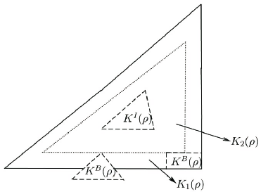
The key idea is to partition into two parts and c.f., Figure 1, build a special function whose bound can be estimated.
Figure 1: The areas surrounded by dashed lines are and respectively. and are separated by dotted lines.
Let and be the oscillatory boundary condition, is the multiscale basis function which is built through the discrete harmonic extension, c.f., (3.3). Accordingly,
We only need to construct a function for which we can estimate its norm. We define the function explicitly by its values at the nodes of
where denotes the set of fine mesh vertexes in
Obviously, the function is contained in
We begin by constructing on each By Assumption 3.1, and that with being the part of locating in Next, we define the values of on then extend to
For simplicity, we assume that lies only in the interior of i.e., does not touch any vertex of For a fixed we may choose local coordinate system and some such that Define for all After defining all the values of on its values at the nodes of for which we set .
Define
where Similarly,
denote the area of which is not contained in Clearly, and hold by their definitions.
We give an upper bound for We note,
For the term we have
From (3.2) and the nodal values defined above we can see that on each where is the coarse edge of . Hence
Let and since on it follows from Assumption 3.1 (3) that
which implies that
For the term let and
be the boundary layer of with width Note that, by definition, we have on
and since on we get
where in the last inequality we have used the fact that since all the nodal values of defined on are between and .
Finally, for the term define
which is the boundary layer of width of and
which is the interior part of
By the definition of , we have on Since on we get
The theorem is proved by combining the upper bounds for and together.
∎
3.3 Upper bound of DG indicator
In this section, we estimate the term Note that, if the coefficient field is continuous across the coarse grid boundaries, we have thus in this case, what we need to focus on is the estimate of the term However, in reality, the coefficient field can be discontinuous across the coarse grid boundaries.
In both cases, suppose the coefficient of the conductivity field satisfies where is a given number, on the edges of fine mesh triangles which intersect with the coarse grid boundaries. Then the indicator yield a bound which is independent of the high contrast in the coefficients.
Theorem 3.4.
For all let the coefficient field be discontinuous across the coarse grid boundaries. If there exists such that then
using the fact that The same result holds for the estimate on Hence, since the theorem is proved.
∎
4 Numerical Experiments
In this section, we present our numerical results,
where we solve the equation (2.1, 2.2) with on the square domain .
We run the preconditioned conjugate gradient method
until the norm of the residual is reduced by a factor of
In the numerical experiments, subdomains are all square shaped,
and each subdomain consists of two coarse triangles.
In each of our numerical experiments below, we consider the performance of our two methods
and compare with the method in [5].
The results of our method are shown in the columns under the heading ”Discontinuous Galerkin”,
while the results from [5] are shown under the heading ”Continuous Galerkin”.
We also use different basis functions for the coarse
space, and that is, the piecewise linear basis function,
the multiscale basis function with linear boundary condition,
and the multiscale basis function with oscillatory boundary condition, respectively.
We choose the same penalty parameter for both the fine and coarse bilinear forms.
Figure 2: The coefficient corresponding to the binary domain of Example 4.1.
Example 4.1.
We begin with our first example here, see Figure 2, where and denotes
a ’binary’ medium with on a square area inclusion lying in the middle of
each coarse grid element and at a distance of both from the horizontal and
the vertical edge of and in the rest of the domain. We study the
behavior of the preconditioners as
For the discontinuous Galerkin formulation, we first consider the nonoverlapping method.
We note that and that
the DG indicator because the coefficient is continuous across the coarse grid boundaries as well as the zero Dirichlet boundary condition.
Taking in Theorem 3.3 implies that
It then follows from Theorem 3.1 that the nonoverlapping method has a bound which is independent of the jumps.
For the overlapping method, we
have thus in this case
the multiscale basis function with linear boundary condition will yield a robust bound.
We note that, in this example, the multiscale basis function with oscillatory boundary condition
is the same as the one with linear boundary condition.
The numerical results in Table 1 show that,
both the nonoverlapping and overlapping method with multiscale coarse basis functions with linear boundary conditions
are robust as predicted by the theory.
The overlapping method [5] with the same multiscale coarse basis functions
produces almost the same condition number estimates, however, for the linear coarsening,
the results in Table 1 show a loss of robustness of the overlapping Schwarz method as goes from to
Table 1: Condition number estimates of the Schwarz methods on Example 4.1 with and .
Discontinuous Galerkin
Continuous Galerkin
Nonoverlapping
Overlapping
Overlapping
26.79
6.43
1.00
5.64
5.6
21.61
6.44
1.42
5.79
58.6
21.49
6.81
1.44
5.80
358.3
21.49
6.81
1.44
5.80
378.7
In our next experiments, we study the behavior with different penalty terms.
As we can see from Table 2,
the condition number estimate for the nonoverlapping method grows linearly with the penalty
parameter However, it is almost constant for the overlapping method,
which suggests that the condition number bound do not depend on the penalty parameter.
The results in Table 2 is in agreement with Theorem 3.1 and Theorem 3.2.
Table 2: Discontinuous Galerkin formulation on Example 4.1. Condition number estimates of the Schwarz method with and
Nonoverlapping method
Overlapping method
33.14
64.88
635.2
6.47
6.56
6.88
26.55
51.09
487.3
6.73
6.87
6.96
26.39
50.74
483.4
6.83
6.89
6.99
26.40
50.73
483.4
6.83
6.89
6.99
Remark 4.1.
Note that, in our numerical experiments, we test the model problem with zero Dirichlet boundary condition, thus all the degrees of freedom are inside domain which means that our DG indicator defined in (3.11) is only for but not for the coarse grid boundaries on Moreover, in Example 4.1, since the coefficient of the conductivity field is continuous across coarse grid boundaries, we have due to the fact that the jump of the coarse basis functions corresponding to the same coarse node is equal to 0. From Theorem 3.1, we know that the condition number bound for the nonoverlapping case will be
taking in Theorem 3.3 we have , thus theoretically speaking, the condition number bound will grow linearly with the penalty parameter While for the overlapping case, From Theorem 3.2, we know that the condition number bound for the overlapping case will be
taking in Theorem 3.3 implies , thus in this case, our condition number bound will keeps unchanged independent of the penalty parameter . Both of the two cases are matched exactly by our numerical experiments in Table 2.
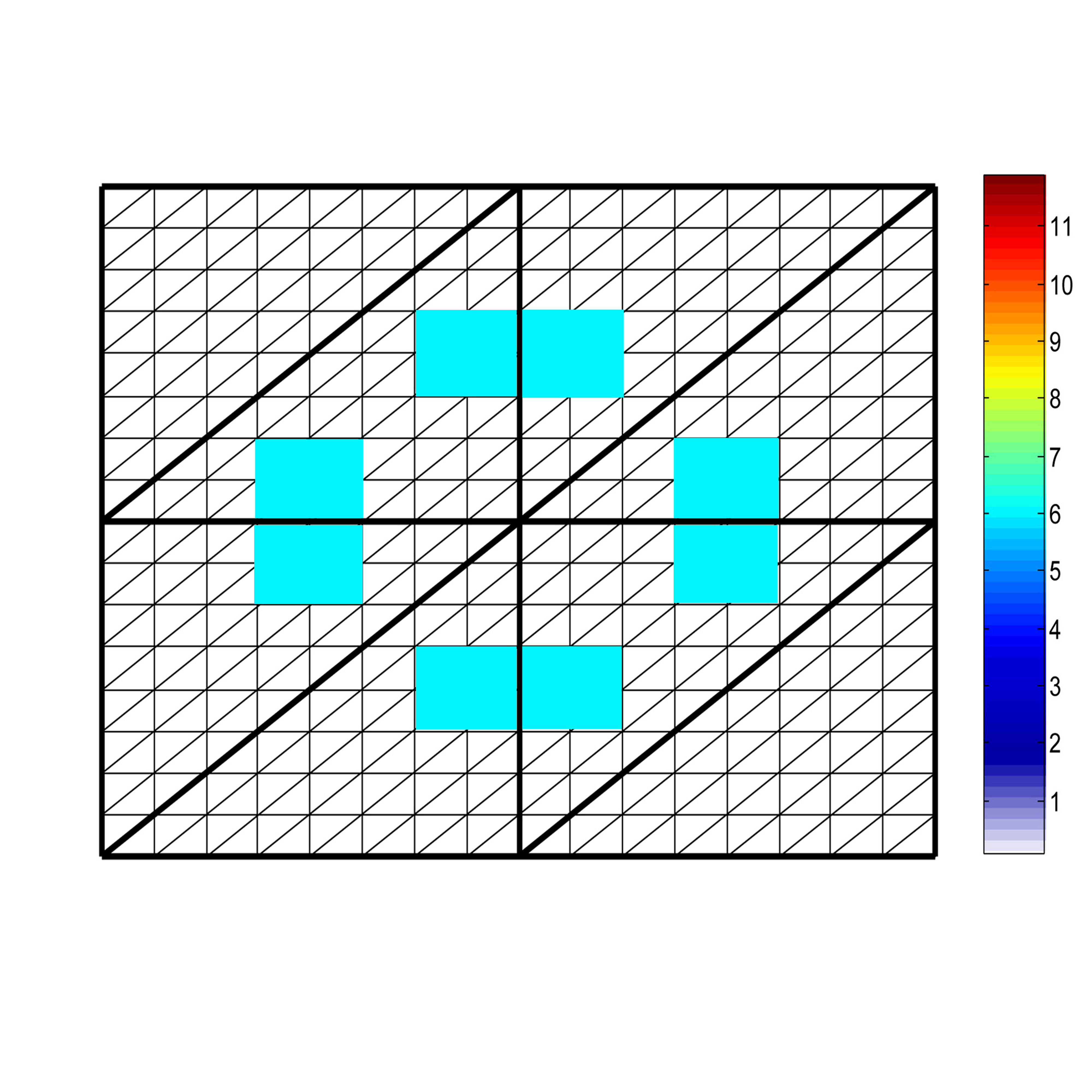
Figure 3: Example 4.2 with crossing the coarse grid boundaries, on the channels and otherwise.
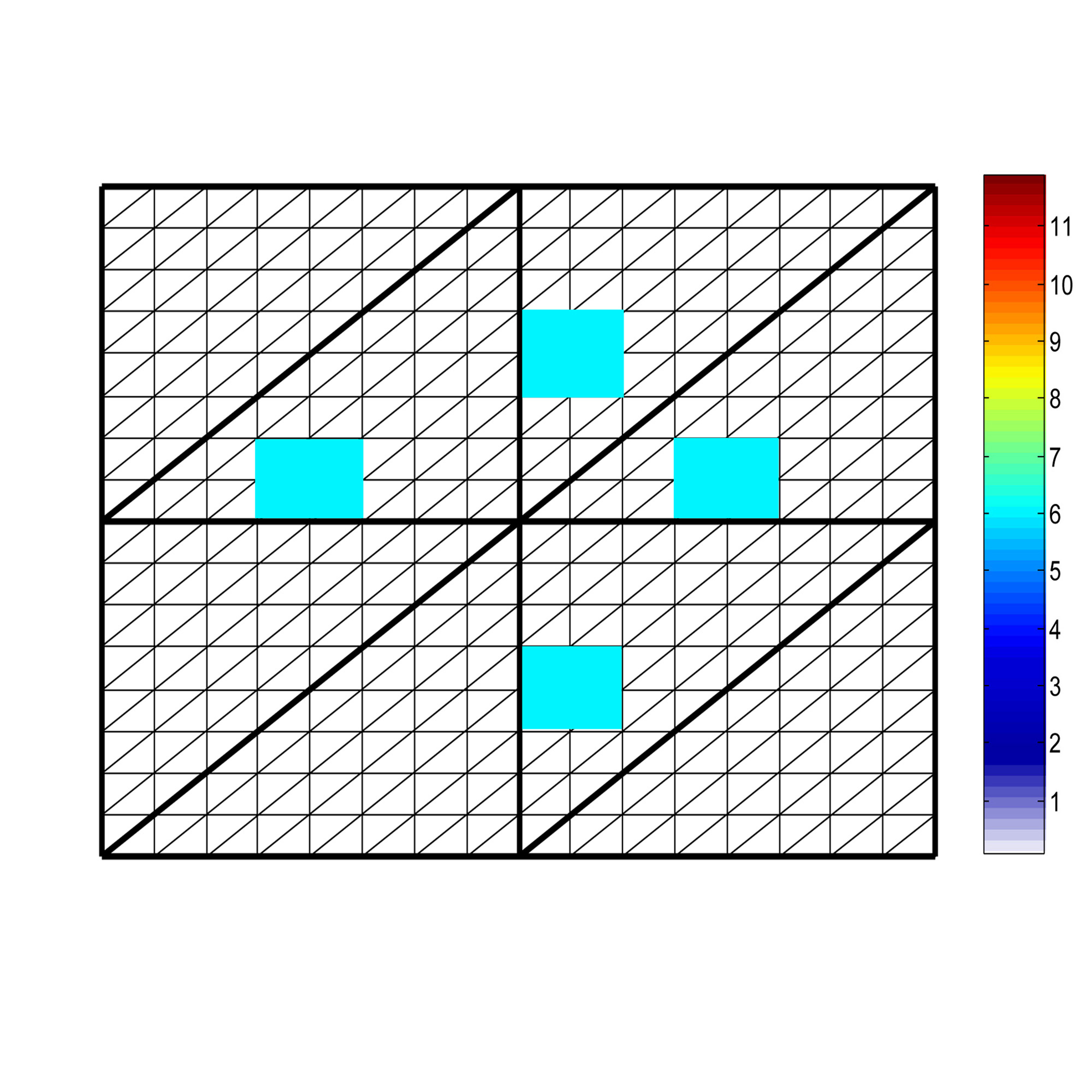
Figure 4: Example 4.2 with touching the coarse grid boundaries, on the channels and otherwise.
Example 4.2.
In this example, the high conductivity field is no longer contained inside,
it touches the coarse grid boundaries, see Figure 3 and Figure 4.
In Figure 3, The conductivity field corresponds to a binary medium with background being equal
to one, and on the channels with an area equal to each.
In Figure 4, the high conductivity channels with diameter are located only on one side of the coarse grid boundaries.
We first compare the behavior of our nonoverlapping method on the two cases shown in Figure 3 and Figure 4.
For the the conductivity field given in Figure 3,
since ,
(taking in Theorem 3.3),
and . Thus Theorem 3.1 predicts that the condition number bound will
grow as
However, for the conductivity field in Figure 4, we
have (taking in Theorem 3.3),
and (taking in Theorem 3.4).
Theorem 3.1 predicts that the bound is robust in this case. For the overlapping method,
it is easy to see
that It
follows from Theorem 3.2 that the condition number bound will be independent of the jumps
for both the conductivity field in Figure 3 and in Figure 4.
The numerical results in Table 3 confirm these results.
Table 3: Discontinuous Galerkin formulation on Example 4.2. Condition number estimates
for the Schwarz method with and the penalty parameter .
Nonoverlapping Overlapping
2.68e+1
26.79
6.23
6.24
5.00e+2
28.91
7.17
7.15
4.76e+4
28.95
7.23
7.17
4.76e+6
28.96
7.23
7.17
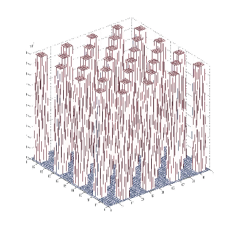
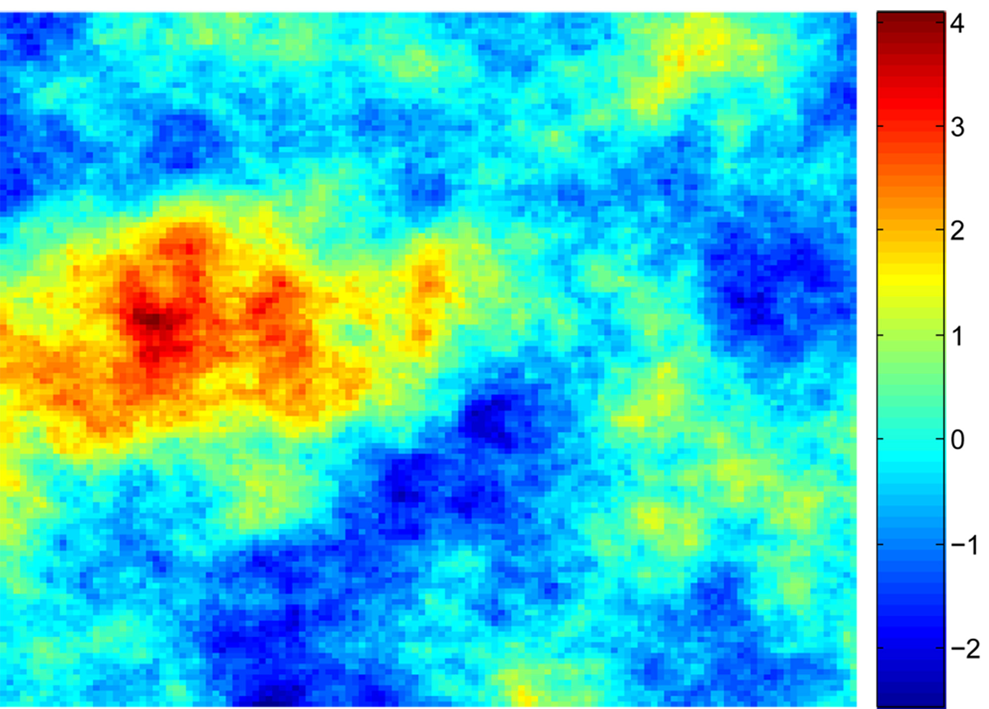
Figure 5: Gaussian random field with covariance parameter
Table 4: Condition numbers (iteration numbers) of Schwarz methods on Example 4.3 with and .
Discontinuous Galerkin
Continuous Galerkin
Nonoverlapping
Overlapping
Overlapping
8.55e+3
7.20 (16)
6.65 (15)
1.75e+5
7.85 (18)
7.12 (16)
7.32e+7
9.86 (21)
8.45 (19)
1.49e+9
11.27 (22)
9.38 (20)
6.02e+11
14.77 (25)
11.73 (22)
1.28e+13
16.80 (26)
13.28 (25)
Example 4.3.
[Gaussian random field] In this example, we test our method on a more realistic model.
The coefficient is a realisation of a log-normal random field (see Figure 5), i.e., is
a realisation of a homogeneous isotropic Gaussian random field with spherical covariance function, mean 0.
This is a commonly studied model in the multiscale area in many literatures [5, 6].
There are some evidences from field data that this gives a reasonable
presentation of reality in certain cases [15, 16].
There are many good ways to generate such random fields, we simply follow
the way in [19] which used FFT (Fast Fourier Transformation) method [17, 18].
The spherical covariance function has a parameter , a bigger increases the correlation
of the random field.
In the numerical experiments, we compared the condition number
estimates (iteration numbers) of both the nonoverlapping and overlapping domain decomposition method
with the method [5].
5 Conclusions
In this paper, we present two two level additive Schwarz domain decomposition methods
for the multiscale second order elliptic problem.
The work here is an extension of related works, c.f., [4, 5], to a discontinuous Galerkin formulation, c.f., [13].
For the nonoverlapping case,
we show that if the conductivity field do not cross the subdomain boundaries, our nonoverlapping method is robust.
However, in some cases, when the conductivity field cross the subdomain boundaries, we show in Theorem 3.1
that our condition number estimate will be dependent on , i.e., the weighted average of the
coefficient over the edge It is now the topic of further investigation to see if we can get rid of this dependence
on . For the overlapping method, as seen in Theorem
3.2, we show that our method is robust under Assumption 3.1. We allow the discontinuity of the coefficients across the coarse grid
boundaries.
Acknowledegments The authors thank Professor Maksymilian Dryja for a fruitful discussion on the paper and, in particular, for his valuable comments on the discontinnuous Galerkin method.
REFERENCES
[1] D. A. Adams, Sobolev Spaces, Academic Press, New York(1975).
[2] Barry F. Smith, Petter Bjørstad, William Gropp, Domain Decomposition: Parallel Multilevel Methods
for Elliptic Partial Differential Equations, Cambridge University Press(1996).
[3] Petter Bjørstad, Maksymilan Dryja, Eero Vainikko, Additive Schwarz Methods without Subdomain Overlap and New Coarse Spaces, Proceedings from the
8th. International conference on domain decomposition methods(1996), John Wiley & Sons(1997).
[4]M. Dryja, M. Sarkis, Additive average Schwarz methods for discretization of elliptic problems with highly discontinuous coefficients,
Computational Methods in Applied Mathematics, 10, 1-13(2010).
[5] I. G. Graham, P. O. Lechner, R. Scheichl, Domain Decomposition for multiscale PDEs, Numer. Math., 589-626(2007).
[6]Cliffe, K. A., Graham, I. G., Scheichl, R., Stals, L., Parallel computation of flow in heterogeneous media modelled by mixed finite elements. J. Comp. Phys., 164, 258-282(2000).
[7] Susanne C. Brenner, L. Ridgway Scott, The mathematical theory of finite element methods, Springer(2002).
[8] Thomas Y. Hou, Xiaohui Wu, Zhiqiang Cai, Convergence of a multiscale finite element method for elliptic problems with rapidly oscillating coefficients, 913-943(1999).
[9] Ivan Lunati, Patrick Jenny, Multiscale finite-volulme method for density-driven flow in porous media, Comput. Geosci., 337-350(2008).
[10] Ivan Lunati, Patrick Jenny, Multiscale finite-volume method for compressible multiphase flow in porous media, Journal of Computational Physics, 616-636(2006).
[11]J. Galvis, Y. Efendiev, Domain decomposition preconditioners for multiscale flows in high-contrast media,
Multiscale Model Simul., 8, 1461-1483(2010).
[12] A. Toselli, O. Widlund, Domain Decomopsition Methods-Algorithm and Theory, Springer-Verlag Berlin Heidelberg(2005).
[13]Zhiqiang Cai, Xiu Ye, Shun Zhang, Discontinuous Galerkin finite element methods for interface
problems: a priori and a posteriori error estimations, SIAM J. Numer. Anal., 49(2011).
[14] Xiaobing Feng, Ohannes A. Karakasshian, Two-level additive Schwarz methods for a discontinous Galerkin approximation of second order elliptic problems, SIAM J. Numer. Anal., 39, 1343-1365(2001).
[15]L. W. Gelhar, A Stochastic Conceptual Analysis of One-Dimensional Groundwater
Flow in Nonuniform Homogeneous Media, Water Resour. Res., 11, 725-741(1975).
[16]R. J. Hoeksema and P. K. Kitanidis, Analysis of the Spatial Structure of Properties
of Selected Aquifers, Water Resour. Res., 21, 563-572 (1985).
[17]Feng Ruan, and Dennis Maclaughlin, An efficient multivariate random field generator using the fast Fourier transform, Advances in Water Resources, 21, 385-399(1998).
[18]M. L. Robin, A. L. Gutjahr, E. A. Sudicky, and J. L. Wilson, Cross-correlated Random
Field Generation with the Direct Fourier Transform Method, Water Resour.
Res., 29 , 2385-2398(1993).
[19]Kozintsev, B., Kedem, B.: Gaussian package, University of Maryland. Available at http://www.
math.umd.edu/ bnk/bak/generate.cgi (1999) Authors address: Yunfei Ma and Xuejun Xu, Institute of Computational Mathematics and Scientific/Engineering
Computing, Academy of Mathematics and Systems Science, Chinese
Academy of Sciences, Beijing 100190, China.
mayf@lsec.cc.ac.cn, xxj@lsec.cc.ac.cn. Petter Bjørstad, Department of Informatics, University of Bergen, Thormøhlensgate 55, 5008 Bergen, Norway.
Petter.Bjorstad@ii.uib.no. Talal Rahman, Faculty of Engineering, Bergen University College,
Nygårdsgaten 112, 5020 Bergen, Norway.
Talal.Rahman@hib.no.
![[Uncaptioned image]](/html/1203.4044/assets/x1.png)