Topological Superfluid Transition Induced by Periodically Driven Optical Lattice

Abstract

We propose a scenario to create topological superfluid in a periodically driven two-dimensional square optical lattice. We study the phase diagram of a spin-orbit coupled s-wave pairing superfluid in a periodically driven two-dimensional square optical lattice. We find that a phase transition from a trivial superfluid to a topological superfluid occurs when the potentials of the optical lattices are periodically changed. The topological phase is called Floquet topological superfluid and can host Majorana fermions.

I INTRODUCTION

Optical lattice system has gradually become a promising platform to study many-body quantum systems because of lots of significant advances in cold-atom experiments Lewe . In particular, recent theoretical and experimental progress in laser-induced-gauge-field Ruse ; Oste ; Juze ; Zhu2 ; Lin1 ; Lin2 makes it a hot spot to study topological quantum states in cold atoms system Stanescu1 ; Bermudez ; Satija ; LXJ2 . Recently, topological quantum states have attracted considerable interest in condensed physics; however, subject to the compounds’ natural properties Stan , we have to rely on serendipity in looking for topological materials in solid-state structures Mura ; Koni ; Hsieh3 ; Zhang . In contrast, one can engineer the Hamiltonian of an optical lattice system to realize variant quantum phase states Gold2 ; Zhu3 ; Liu .

In this paper, we show that periodically driven perturbations may give rise to a phase transition from a trivial superfluid to a topological one, which carries the hallmark with topological protected gapless edges on the boundaries of the system. Time-periodic dependent Hamiltonian can be described by Floquet’s theorem, which is used to explain quantized adiabatic pumping phenomena Fu ; Inoue1 ; Thouless ; Niu . Recently, it demonstrated that the phase transition from a superfluid to a Mott insulator in one-dimensional Bose-Hubbard model can be induced by a periodically driven optical lattice Ecka . We extend this phase transition mechanism to explore the topological phase transition in a two-dimensional optical lattice. We study the phase diagram of a spin-orbit coupled s-wave pairing superfluid in a periodically driven two-dimensional (2D) square optical lattice. We find that a topological phase transition from a trivial superfluid to a topological superfluid can be induced in periodically modulated optical lattices. The topological phase is called Floquet topological superfluid Jiang ; Kita ; Inoue2 ; Lind ; Kita2 and can host Floquet Majorana fermions. It was proposed that a topological phase can be realized in a BCS s-wave superfluid of ultracold fermionic atoms in the presence of both a Rashba spin-orbit (SO) interaction and a large perpendicular Zeeman field Sato ; ZhangPRL ; ZhangPRA ; Zhu4 ; however, the Rashba spin-orbit coupling and a large perpendicular Zeeman field are hard to be simultaneously realized for cold fermionic atoms ZhangPRA ; Zhu4 . We will prove that if one replaces the Zeeman field by a periodically driven optical lattice Ecka , a spin-orbit coupled BCS s-wave superfluid will still allow a realization of topological superfluid through modifying the oscillating amplitude (or modulation strength) of optical lattice. Therefore, we provide an alternative method to create an important topological superfluid which can host Majorana fermions.

The paper is organized as follows: In Sec. II, we introduce the s-wave superfluid model in a square optical lattice in the presence of both a Rashba SO coupling and a periodically modulated optical lattice potential. A Zeeman-magnetic-field-like term will be derived under the first order approximation; In Sec. III we present a two-band approximation and explain the topological phase transition at the $\Gamma$ point in the first Brillouin zone (BZ). At last, we give a brief summary in Sec. IV.

II MODEL

The tight-binding Hamiltonian, which describes an s-wave superfluid of neutral fermionic atoms in a 2D optical square lattice, is given by

$$H\left(t\right)=H_{0}+H_{d}\left(t\right),$$ (1)

where

$$H_{0} =-t\sum_{\langle ij\rangle}c_{i}^{{\dagger}}c_{j}-i\lambda\sum_{\langle ij\rangle}c_{i}^{{\dagger}}\left(\mathbf{\sigma\times\hat{d}}_{ij}\right)_{z}c_{j}$$

$$+\mu\sum_{i}c_{i}^{{\dagger}}c_{i}+U\sum_{i}c_{i\uparrow}^{{\dagger}}c_{i\downarrow}^{{\dagger}}c_{i\downarrow}c_{i\uparrow},$$ (2)

and

$$H_{d}\left(t\right)=\mathbf{K}\left(t\right)\cdot\sum_{i}\mathbf{r}_{i}c_{i}^{{\dagger}}c_{i}.$$ (3)

Here $t$ is the hopping amplitude between the nearest neighbor link $\langle i,j\rangle$, $c_{i}^{{\dagger}}$=$\left(c_{i\uparrow}^{{\dagger}},c_{i\downarrow}^{{\dagger}}\right)$ with $c_{i\alpha}^{{\dagger}}$ ($c_{i\alpha}$) denoting the creation (annihilation) operator of a fermionic atom with pseudospin $\alpha$ (up or down) on lattice site $i$. The second term in Eq. (2) represents a Rashba SO coupling interaction which can be obtain by laser-induced-gauge-field method, $\lambda$ is the coupling coefficient, $\mathbf{\sigma}$ are the Pauli matrices and $\mathbf{\hat{d}}_{ij}$ is a unit vector along the bond that connects site $j$ to $i$. $\mu$ is the chemical potential and $U<0$ denotes an on-site attractive interaction which is easy to obtain via an s-wave Feshbach resonance in cold atom system. The oscillating Hamiltonian $H_{d}$, with $\mathbf{K}\left(t\right)=K\left(\cos\left(\omega t\right),\sin\left(\omega t\right)\right)$, mimics a monochromatic electric dipole potential with frequency $\omega$ and amplitude $K$. This term can be realized experimentally by periodically shifting the position of a mirror employed to generate the standing laser waves along $x$- and $y$-directions, and transforming to the comoving frame of reference Ecka . We choose $t$=$1$ as the energy unit and the distance $a$ between the nearest sites as the length unit throughout this paper. It was demonstrated in Ref. Sato that the Hamiltonian $H_{0}$ in a mean field approximation and combination with a perpendicular Zeeman field can support a topological superfluid. On the other hand, replaced the Hamiltonian $H_{0}$ with an one-dimensional Bose-Hubbard Hamiltonian, it was shown in Ref. Ecka that a phase transition from a superfluid to a Mott insulator can be induced by $H_{d}$ in its one-dimensional form.

When a Hamiltonian of quantum system has a periodic dependence on time, i.e., $H\left(t\right)$=$H\left(t+T\right)$ with period $T$=$2\pi/\omega$, the Hamiltonian satisfies the discrete time translational symmetry, $t\rightarrow t+T$, which can been described by Floquet’s theorem Ecka ; Shirl ; Grif . Floquet’s theorem tell us that the Schrödinger equation with time-periodic dependent Hamiltonian has a complete set of solutions with the form $\left|\psi_{n}\left(t\right)\right\rangle$=$\left|u_{n}\left(t\right)\right\rangle\exp\left(-i\varepsilon_{n}t/\hbar\right)$. Here, the periodic function $\left|u_{n}\left(t\right)\right\rangle=\left|u_{n}\left(t+T\right)\right\rangle$, an analog of Bloch states known from spatially periodic crystals, satisfies the eigenvalue equation

$$\left[H\left(t\right)-i\hbar\partial_{t}\right]\left|u_{n}\left(t\right)\right\rangle=\varepsilon_{n}\left|u_{n}\left(t\right)\right\rangle.$$ (4)

We call $\mathcal{H}\left(t\right)$=$H\left(t\right)-i\hbar\partial_{t}$ as the Floquet Hamiltonian and the eigenvalues $\varepsilon_{n}$ as quasienergies which are defined modulo the frequency $\omega$=$2\pi/T$.

The Floquet basis

$$\left|\left\{n_{i}\right\},m\right\rangle=\left|\left\{n_{i}\right\}\right\rangle\exp\left[\mathtt{-}\frac{i}{\hbar\omega}\int_{-\infty}^{t}dt^{\prime}\mathbf{K}\left(t^{\prime}\right)\mathtt{\cdot}\sum_{i}\mathbf{r}_{i}n_{\mathbf{i}}\mathtt{+}im\omega t\right],$$ (5)

where $\left|\left\{n_{i}\right\}\right\rangle$ indicates a Fock state with $n_{i}$ particles on the $i$th site, and $m$ accounts for the zone structure Ecka , consist of an extended Hilbert space of $T$-periodic functions with the scalar product given by

$$\left\langle\left\langle\cdot\mathtt{\mid}\cdot\right\rangle\right\rangle=\frac{1}{T}\int_{0}^{T}dt\left\langle\cdot\mathtt{\mid}\cdot\right\rangle,$$ (6)

i.e., by the usual scalar product $\left\langle\cdot\mathtt{\mid}\cdot\right\rangle$ combined with time-averaging. Hence, the quasienergies are obtained by computing the matrix elements of the Floquet operator $H\left(t\right)-i\hbar\partial_{t}$ in the basis (5) with respect to the scalar product (6), and diagonalizing. By a straightforward calculation, we can obtain the matrix elements of some operators in Floquet Hamiltonian $\mathcal{H}\left(t\right)$:

$$\left\langle\left\langle\left\{n_{i}^{\prime}\right\},m^{\prime}\right|c_{i\alpha}^{{\dagger}}c_{j\alpha^{\prime}}\left|\left\{n_{i}\right\},m\right\rangle\right\rangle=e^{-i\left(m^{\prime}-m\right)\theta_{ij}}J_{m^{\prime}-m}\left(z_{ij}\right),$$ (7)

$$\left\langle\left\langle\left\{n_{i}^{\prime}\right\},m^{\prime}\right|c_{i\alpha}^{{\dagger}}c_{i\alpha}\left|\left\{n_{i}\right\},m\right\rangle\right\rangle=n_{i\alpha}\delta_{m,m^{\prime}},$$ (8)

$$\left\langle\left\langle\left\{n_{i}^{\prime}\right\},m^{\prime}\right|c_{i\uparrow}^{{\dagger}}c_{i\downarrow}^{{\dagger}}c_{i\downarrow}c_{i\uparrow}\left|\left\{n_{i}\right\},m\right\rangle\right\rangle=n_{i\uparrow}n_{i\downarrow}\delta_{m,m^{\prime}},$$ (9)

where $J_{m^{\prime}-m}\left(z_{ij}\right)$ is the Bessel function of the $\left(m^{\prime}-m\right)$th order and $z_{ij}$=$\frac{K}{\hbar\omega}\sqrt{x_{ij}^{2}+y_{ij}^{2}}$. Here, $x_{ij}=\left(\mathbf{r}_{i}\right)_{x}-\left(\mathbf{r}_{j}\right)_{x}$, $y_{ij}=\left(\mathbf{r}_{i}\right)_{y}-\left(\mathbf{r}_{j}\right)_{y}$ and $\tan\theta_{ij}=x_{ij}/y_{ij}$. In the above matrix, the diagonal block of the Floquet Hamiltonian, $\mathcal{H}^{\left(mm\right)}$, is the $n$-photon sector, i.e., the subspace with $n$ photons and the non-diagonal blocks $\mathcal{H}^{\left(m^{\prime}m\right)}$ with $m^{\prime}\neq m$ correspond to the interaction between different subspaces Inoue2 . For sufficiently high frequencies, we can argue, from Eq. (7-9), that the driven system (1) behaves similar to the undriven system (2), but with the tunneling matrix element $t$ and the SO coupling $\lambda$ of the latter being replaced by the effective matrix element $t\sim tJ_{0}\left(z_{ij}\right)$ and $\lambda\sim\lambda J_{0}\left(z_{ij}\right)$, respectively. Now, suppose that we enhance the modulation strength $K$, then we have to consider the coupling of other photon sectors. For simplify, we only consider coefficient of subspace with $n=1$ photon on the subspace with $n=0$ photon. When $K$ is strong enough but still satisfy $z_{ij}<<1$, the system has the effective Hamiltonian Kita2

$$\mathcal{H}_{eff}=\mathcal{H}^{\left(00\right)}+\frac{1}{\hbar\omega}\left[\mathcal{H}^{-1},\mathcal{H}^{+1}\right].$$ (10)

Here, $\mathcal{H}^{-1}$ ($\mathcal{H}^{+1}$) denotes the non-diagonal block with $m\prime-m=-1$ $\left(+1\right)$ around the $0$-photon sector. According to Eqs. (7-9), we can obtain

$$\mathcal{H}^{\left(00\right)} =-t\sum_{\langle ij\rangle}J_{0}\left(z_{ij}\right)c_{i}^{{\dagger}}c_{j}-i\lambda\sum_{\langle ij\rangle}J_{0}\left(z_{ij}\right)c_{i}^{{\dagger}}\left(\mathbf{\sigma\times\hat{d}}_{ij}\right)_{z}c_{j}$$

$$+\mu\sum_{i}c_{i}^{{\dagger}}c_{i}+\psi_{s}\sum_{i}\left(c_{i\uparrow}^{{\dagger}}c_{i\downarrow}^{{\dagger}}+\text{H.c.}\right),$$ (11)

$$\mathcal{H}^{-1} =-t\sum_{\langle ij\rangle}e^{i\theta_{ij}}J_{-1}\left(z_{ij}\right)c_{i}^{{\dagger}}c_{j}$$

$$-i\lambda\sum_{\langle ij\rangle}e^{i\theta_{ij}}J_{-1}\left(z_{ij}\right)c_{i}^{{\dagger}}\left(\mathbf{\sigma\times\hat{d}}_{ij}\right)_{z}c_{j},$$ (12)

$$\mathcal{H}^{+1} =-t\sum_{\langle ij\rangle}e^{-i\theta_{ij}}J_{+1}\left(z_{ij}\right)c_{i}^{{\dagger}}c_{j}$$

$$-i\lambda\sum_{\langle ij\rangle}e^{-i\theta_{ij}}J_{+1}\left(z_{ij}\right)c_{i}^{{\dagger}}\left(\mathbf{\sigma\times\hat{d}}_{ij}\right)_{z}c_{j}.$$ (13)

In the derivation of Eq. (11), we have made a mean field approximation and $\psi_{s}$ is the gap function.

By using the Fourier transform of atomic operators $c_{i\sigma}^{{\dagger}}$, i.e.,

$$\ c_{i\sigma}^{{\dagger}}=\frac{1}{\sqrt{N}}\sum_{\mathbf{k}}c_{\mathbf{k}\sigma}^{{\dagger}}e^{-i\mathbf{k\cdot R}_{i}},$$ (14)

the Hamiltonian (10) in square lattice system can be rewritten in the momentum space as

$$\mathcal{H}_{eff}=\sum_{\mathbf{k}}\psi_{\mathbf{k}}^{+}(\mathcal{H}_{eff}(\mathbf{k})\psi_{\mathbf{k}},$$ (15)

where we have defined the four-component basis operator $\psi_{\mathbf{k}}$=$(c_{\mathbf{k}\uparrow},c_{\mathbf{k}\downarrow},c_{-\mathbf{k}\uparrow}^{{\dagger}},c_{-\mathbf{k}\downarrow}^{{\dagger}})^{\text{T}}$. The effective Hamiltonian in momentum space is given by

$$\mathcal{H}_{eff}(\mathbf{k})=\left(\begin{array}[c]{cccc}\varepsilon_{\mathbf{k}}-\Gamma\left(\mathbf{k},z\right)&2\lambda J_{0}\left(z\right)\alpha\left(\mathbf{k}\right)&0&\psi_{s}\\ 2\lambda J_{0}\left(z\right)\alpha^{\ast}\left(\mathbf{k}\right)&\varepsilon_{\mathbf{k}}+\Gamma\left(\mathbf{k},z\right)&-\psi_{s}&0\\ 0&-\psi_{s}&-\varepsilon_{-\mathbf{k}}+\Gamma\left(\mathbf{k},z\right)&2\lambda J_{0}\left(z\right)\alpha^{\ast}\left(\mathbf{k}\right)\\ \psi_{s}&0&2\lambda J_{0}\left(z\right)\alpha\left(\mathbf{k}\right)&-\varepsilon_{-\mathbf{k}}-\Gamma\left(\mathbf{k},z\right)\end{array}\right),$$ (16)

where $\alpha\left(\mathbf{k}\right)=\sin k_{y}+i\sin k_{x},z=\frac{Ka}{\hbar\omega},\Gamma\left(\mathbf{k},z\right)=\frac{16\lambda^{2}J_{+1}\left(z\right)J_{-1}\left(z\right)}{\hbar\omega}\cos k_{x}\cos k_{y}$, and $\varepsilon_{\mathbf{k}}=-2tJ_{0}\left(z\right)\left(\cos k_{x}+\cos k_{y}\right)-\mu$. Following the method outlined in Ref. Sato , one can obtain a “dual” Hamiltonian

$$\mathcal{H}^{D}\left(\mathbf{k}\right)=\left(\begin{array}[c]{cccc}\psi_{s}-\Gamma\left(\mathbf{k},z\right)&2\lambda J_{0}\left(z\right)\alpha\left(\mathbf{k}\right)&0&-\varepsilon_{\mathbf{k}}\\ 2\lambda J_{0}\left(z\right)\alpha^{\ast}\left(\mathbf{k}\right)&-\psi_{s}+\Gamma\left(\mathbf{k},z\right)&\varepsilon_{\mathbf{k}}&0\\ 0&\varepsilon_{\mathbf{k}}&\psi_{s}+\Gamma\left(\mathbf{k},z\right)&-2\lambda J_{0}\left(z\right)\alpha^{\ast}\left(\mathbf{k}\right)\\ -\varepsilon_{\mathbf{k}}&0&-2\lambda J_{0}\left(z\right)\alpha\left(\mathbf{k}\right)&-\psi_{s}-\Gamma\left(\mathbf{k},z\right)\end{array}\right),$$ (17)

where the unitary transformation $\mathcal{H}^{D}\left(\mathbf{k}\right)=DH_{eff}D^{{\dagger}}$ with

$$D=\frac{1}{\sqrt{2}}\left(\begin{array}[c]{cccc}1&0&0&1\\ 0&1&-1&0\\ 0&1&1&0\\ -1&0&0&1\end{array}\right).$$

It is easy to obtain the eigenvalues of Eq. (17) with

$$E_{1} =-\sqrt{f_{1}+f}_{2};E_{2}=-\sqrt{f_{1}-f_{2}},$$

$$E_{3} =+\sqrt{f_{1}-f_{2}};E_{4}=+\sqrt{f_{1}+f_{2}},$$

where we have defined

$$f_{1} =\Gamma^{2}\left(\mathbf{k},z\right)+\left(\varepsilon_{\mathbf{k}}^{2}+\psi_{s}^{2}\right)+4J_{0}^{2}\left(z\right)\lambda^{2}\left|\alpha\left(\mathbf{k}\right)\right|^{2},$$

$$f_{2} =2\sqrt{\Gamma^{2}\left(\mathbf{k},z\right)\left(\varepsilon_{\mathbf{k}}^{2}+\psi_{s}^{2}\right)+4\lambda^{2}J_{0}^{2}\left(z\right)\varepsilon_{\mathbf{k}}^{2}\left|\alpha\left(\mathbf{k}\right)\right|^{2}}.$$

It is obvious that if only $\psi_{s}\neq 0$, i.e., the system lies in the superfluid phase, the energy levels $E_{1}$ and $E_{4}$, denoting the lowest and the highest band, will not touch each other. Next, we discuss the levels $E_{1}$ and $E_{2}$ (or $E_{3}$ and $E_{4}$). These two levels can touch each other if only the following two relations

$$\Gamma^{2}\left(\mathbf{k},z\right)=0$$

and

$$J_{0}^{2}\left(z\right)\varepsilon_{\mathbf{k}}^{2}\left(\sin^{2}k_{x}+\sin^{2}k_{y}\right)=0.$$

are simultaneously satisfied. From $\Gamma^{2}\left(\mathbf{k},z\right)=0$, we have $k_{x}=\pm\frac{\pi}{2}$ or $k_{y}=\pm\frac{\pi}{2}$ in the first BZ. So, when $J_{0}\left(z\right)\neq 0$, we have

$$-\mu=2tJ_{0}\left(z\right)\left(\cos k_{x}+\cos k_{y}\right).$$

When $-\mu>\left|2tJ_{0}\left(z\right)\right|$, the levels $E_{1}$ and $E_{2}$ (or $E_{3}$ and $E_{4}$) will not touch each other for ever. Else, when $-\left|2tJ_{0}\left(z\right)\right|\leq-\mu\leq\left|2tJ_{0}\left(z\right)\right|$, $E_{1}$ and $E_{2}$ (or $E_{3}$ and $E_{4}$) will touch each other at points $\left(k_{x}=\pm\frac{\pi}{2},k_{y}=\arccos\left(\frac{-\mu}{2tJ_{0}\left(z\right)}\right)\right)$ and $\left(k_{x}=\arccos\left(\frac{-\mu}{2tJ_{0}\left(z\right)}\right),k_{y}=\pm\frac{\pi}{2}\right)$. In the following, we only consider the case, $-\mu>\left|2tJ_{0}\left(z\right)\right|$, which means bands $E_{1}$ and $E_{4}$ will be off away from the other two levels $E_{2}$ and $E_{3}$, and then the topological properties of bands $E_{1}$ and $E_{4}$ will not change if we vary some parameters. Therefore, we will only consider the topological properties of band $E_{2}$ and $E_{3}$, which have chances to contact each other at the high symmetry points, $\mathbf{K}_{i=1,...,4}=\left(0,0\right);\left(0,\pi\right);\left(\pi,0\right);\left(\pi,\pi\right)$ in the first BZ, when satisfying the condition

$$\Gamma^{2}\left(z\right)=\varepsilon_{\mathbf{K}_{i}}^{2}+\psi_{s}^{2},$$ (18)

because band-gap closing is an essential condition for the topological characteristic changes. We denote $\Gamma_{\mathbf{K}_{i}}^{2}\left(\mathbf{K}_{i},z\right)=\left(16\lambda^{2}J_{+1}^{2}\left(z\right)/\hbar\omega\right)^{2}=\Gamma^{2}\left(z\right)$. Considering $z<<1$ and $-\mu>\left|2tJ_{0}\left(z\right)\right|$, the two bands can only touch at point $\mathbf{K}_{1}=\left(0,0\right)$ when varying the parameter $z$.

III Topological phase transition

We now study the topological properties of these two bands by two-band approximation at point $\mathbf{K}_{1}=\left(0,0\right)$ in the first BZ. We will not consider the other points since the gaps at other high symmetry points will not shut down, leaving no influence to the topological changes. To have a basic idea of the topological features of the system, we explore it by using a two-band approximation at point $\mathbf{K}_{1}$ in the first BZ. We expand the Hamiltonian (17) at point $\mathbf{K}_{1}$ and obtain

$$\mathcal{H}_{\mathbf{K}_{1}}^{D}\left(\mathbf{q}\right)=\left(\begin{array}[c]{cccc}\psi_{s}+\Gamma\left(z\right)&2\lambda J_{0}\left(z\right)q_{+}&0&4tJ_{0}\left(z\right)+\mu\\ 2\lambda J_{0}\left(z\right)q_{-}&-\left(\psi_{s}+\Gamma\left(z\right)\right)&-\left(4tJ_{0}\left(z\right)+\mu\right)&0\\ 0&-\left(4tJ_{0}\left(z\right)+\mu\right)&\psi_{s}-\Gamma\left(z\right)&-2\lambda J_{0}\left(z\right)q_{-}\\ 4tJ_{0}\left(z\right)+\mu&0&-2\lambda J_{0}\left(z\right)q_{+}&-\left(\psi_{s}-\Gamma\left(z\right)\right)\end{array}\right)$$ (19)

with $q_{\pm}$=$q_{y}\pm iq_{x}$. Because $\psi_{s}<0$ and $\Gamma\left(z\right)>0$, when taking $\left|4tJ_{0}\left(z\right)+\mu\right|\ll 1$, we can see that the major contribution to bands $E_{2}$ and $E_{3}$ comes from the up-diagonal sector in above matrix and thus we may treat the others as a perturbation. Under this condition, we obtain an effective two-band Hamiltonian given by

$$\mathcal{H}_{eff}^{\mathbf{K}_{1}}\left(\mathbf{q}\right)=2\lambda J_{0}\left(z\right)q_{y}\sigma_{x}-2\lambda J_{0}\left(z\right)q_{x}\sigma_{y}+M\left(z\right)\sigma_{z},$$ (20)

where the corresponding mass term $M\left(z\right)$=$\psi_{s}+\Gamma\left(z\right)+\left(4tJ_{0}\left(z\right)+\mu\right)^{2}/\left(\psi_{s}-\Gamma\left(z\right)\right)$ and $\sigma_{\nu=x,y,z}$ the Pauli matrices. Let $M\left(z\right)$=$0$, we obtain the gapless condition Eq. (18) again at $\mathbf{K}_{1}$ point. Eq.(20) can be written as $\mathcal{H}_{eff}^{\mathbf{K}_{1}}\left(\mathbf{q}\right)={\mathbf{\sigma}}\cdot\mathbf{d}$, where the vector $\mathbf{d}=\{2\lambda J_{0}\left(z\right)q_{y},-2\lambda J_{0}\left(z\right)q_{x},M\left(z\right)\}$. The topological features of the system can be characterized by the winding number ( first Chern number) of the Berry phase gauge field $C=\frac{1}{4\pi}\int dk_{x}\int dk_{y}\mathbf{\hat{d}}\cdot(\frac{\partial\mathbf{\hat{d}}}{\partial{k_{x}}}\times\frac{\partial\mathbf{\hat{d}}}{\partial k_{y}})$ in the first Brillouin zone, where $\mathbf{\hat{d}}=\mathbf{d}/|\mathbf{d}|$. When $M\left(z\right)\neq 0$, it is straightforward to obtain the winding number for the effective system described by Eq. (20), i.e.,

$$C=\frac{1}{2}\text{sign}\left(M\left(z\right)\right).$$ (21)

This non-integral winding number appears since the deviations from this two-band approximation model at large momenta are not included in the above calculation of the winding number. So it can not be directly related to the topological features of the system; however, the change in the winding numbers is independent of the large-momentum contribution Qi . Let us discuss the change of the topological properties of superfluid system when we adjust the oscillating amplitude $K$ of optical lattice. It is obvious that the initial non-driven system is in a trivial state which corresponds to $z=0$ and $M\left(z\right)<0$. Now, we apply the driven field to the system and make $M\left(z\right)<0$ to $M\left(z\right)>0$, the change in Chern number is:

$$\Delta C=\frac{1}{2}\left[\text{sign}\left(M\left(z\right)_{>0}\right)-\text{sign}\left(M\left(z\right)_{<0}\right)\right]=+1.$$ (22)

So, we get a topological superfluid state with $C=+1$ for $M\left(z\right)>0$ .

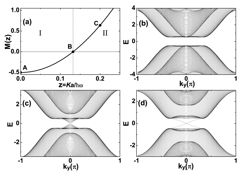
Figure 1: The phase diagram and the band structures of the system. (a) The mass $M\left(z\right)$ as a function of $z$. The region $I$ with $\left(z\right)<0$ is a trivial superfluid, while the region $II$ with $M\left(z\right)>0$ is a topological superfluid. The band structures of the effective Hamiltonian (10) in a striped geometry with 60 sites in $x$ direction are shown in (b), (c) and (d) corresponding to the points A ($z=0$), B ($z=0.132$), and C ($z=0.2$) in (a), respectively. Other parameters $t=1,\lambda=0.6,\psi_{s}=-0.5,\hbar\omega=0.05,$ and $\mu=-4$.

It is notable that gapless chiral edge states are usually the hallmark of a topological system. Therefore, to further prove the above argument, we show the phase diagram and the band structures of the effective Hamiltonian (10) in a striped geometry in Fig. 1. In Fig. 1(a), we plot the mass $M\left(z\right)$ as a function of $z$, which can be adjusted by changing the modulation strength $K$. The point B denotes $M\left(z\right)=0$ with $z=0.1320$, where the bands $E_{2}$ and $E_{3}$ contact each other at $\Gamma$ point. The band structures in a striped geometry with $60$ sites in $x$ direction are shown in (b), (c) and (d) corresponding to the points A ($z=0$), B ($z=0.132$), and C ($z=0.2$) in Fig.(a), respectively. In the numerical calculation, we take the typical parameters $t=1,\lambda=0.6,\psi_{s}=-0.5,\hbar\omega=0.05,$ and $\mu=-4$. It is clear that there is no edge state in the region $I$ where the mass $M\left(z\right)<0$ with $0\leq z<0.1320$, so it is a trivial superfluid. In contrast, there are a pair of edge states in the region $II$ where the mass $M\left(z\right)>0$ with $z>0.1320$, so it is a topological superfluid. There is a phase transition from a trivial superfluid to a topological superfluid occurs at the point $\mathbf{B}$ where the gap is closed.

Generally, there exists Majorana Fermionic excitation bounded with the vortex structure in the nontrivial topological superfluid phase. Hence, we can obtain the 2-D Foquet Majorana fermions Jiang if there have the vortex structures in our system. The vortex structure can be produced from two different routes, one of which can be realized through the phase twist of the SO-produced lasers: $\lambda\rightarrow\lambda e^{im\theta}$ with $m$ the vorticity Sato . Another route is that the vortex structure can come from initial rotation of the atomic cloud Zwierlein . Then the vortex structure is coupled with the superfluid order parameter: $\psi_{s}\rightarrow\psi_{s}e^{im\theta}$, which is similar with the case in the topological superconductor Sau . Both cases give the similar Majorana fermion obviously confirmed from the Eq. (16) and Eq. (17) connected by the unitary transformation $D$. The zero mode solutions of the Majorana fermion can be obtained from the Bogoliubov-de Gennes (BdG) equation, which has the similar form compared with that in Ref. Sato . Moreover, such Majorana fermion excitations can be detected by the standard Raman spectroscopy Tewari ; Zhu4 .

IV CONCLUSION

In summary, we have discussed the topological superfluid phase transition in a periodically driven square optical lattice. By using Floquet’s theorem, we find that a Floquet topological superfluid will be created when the two-dimensional square optical lattice potentials are periodically driven. This topological phase is interesting in hosting a Majorana fermion excitation which can be detected by Raman spectroscopy in cold atom system. Therefore we propose a novel scenario to create Majorana fermions which may play a key role in topological quantum computation.

References

• (1) M. Lewenstein, A. Sanpera, V. Ahufinger, B. Damski, A. Sen(De), U. Sen, Adv. Phys. 56, 243 (2007).
• (2) J. Ruseckas, G. Juzeliūnas, P. Öhberg, and M. Fleischhauer, Phys. Rev. Lett. 95, 010404 (2005).
• (3) K. Osterloh, M. Baig, L. Santos, P. Zoller, and M. Lewenstein, Phys. Rev. Lett. 95, 010403 (2005).
• (4) G. Juzeliūnas, J. Ruseckas, P. Öhberg, and M. Fleischhauer, Phys. Rev. A 73, 025602 (2006).
• (5) S. L. Zhu, H. Fu, C. J. Wu, S. C. Zhang, and L. M. Duan, Phys. Rev. Lett. 97, 240401 (2006); S. L. Zhu, D. W. Zhang, and Z. D. Wang, Phys. Rev. Lett. 102, 210403 (2009).
• (6) Y. J. Lin, R. L. Compton, A. R. Perry, W. D. Phillips, J.V. Porto, and I. B. Spielman, Phys. Rev. Lett. 102, 130401 (2009).
• (7) Y. J. Lin, R. L. Compton, K. Jiménez-García, J. V. Porto, and I. B. Spielman, Nature 462, 628 (2009).
• (8) T. D. Stanescu, V. Galitski, J. Y. Vaishnav, C. W. Clark, and S. Das Sarma, Phys. Rev. A 79, 053639 (2009).
• (9) A. Bermudez, N. Goldman, A. Kubasiak, M. Lewenstein and M. A. Martin-Delgado, New J. Phys. 12, 033041 (2010).
• (10) I. I. Satija, D. C. Dakin, J. Y. Vaishnav, and C. W. Clark, Phys. Rev. A 77, 043410 (2008).
• (11) X. J. Liu, X. Liu, C. Wu, and J. Sinova, Phys. Rev. A 81, 033622 (2010).
• (12) T. D. Stanescu, V. Galitski, and S. D. Sarma, arXiv:0912.3559v1.
• (13) S. Murakami, Phys. Rev. Lett. 97, 236805 (2006).
• (14) M. König, S. Wiedmann, C. Breüne, A. Roth, H. Buhmann, L. W. Molenkamp, X. L. Qi, S. C. Zhang, Science 318, 766 (2007).
• (15) D. Hsieh, D. Qian, L. Wray, Y. Xia, Y. S. Hor, R. J. Cava and M. Z. Hasan, Nature 452, 970 (2008).
• (16) H. Zhang, C. X. Liu, X. L. Qi, X. Dai, Z. Fang, and S. C. Zhang, Nature physics 5, 438 (2009); X. L. Qi, R. Li, J. Zang, S. C. Zhang, Science 323, 1184 (2009).
• (17) N. Goldman, I. Satija, P. Nikolic, A. Bermudez, M. A. Martin-Delgado, M. Lewenstein, and I. B. Spielman, arXiv: 1002.0219v2; A. Bermudez, L. Mazza, M. Rizzi, N. Goldman, M. Lewenstein, and M. A. Martin-Delgado, arXiv: 1004.5101v1.
• (18) L. B. Shao, S. L. Zhu, L. Sheng, D.Y. Xing, and Z. D. Wang, Phys. Rev. Lett. 101, 246810 (2008).
• (19) G. Liu, S. L. Zhu, S. Jiang, F. Sun, and W. M. Liu, Phys. Rev. A 82, 053605 (2010).
• (20) L. Fu and C. L. Kane, Phys. Rev. B 74, 195312 (2006).
• (21) J. I. Inoue, Phys. Rev. B 81, 125412 (2010).
• (22) D. J. Thouless, Phys. Rev. B 27, 6083 (1983).
• (23) Q. Niu and D. J. Thouless, J. Phys. A 17, 2453 (1984); S. L. Zhu and Z. D. Wang, Phys. Rev. B 65, 155313 (2002)
• (24) A. Eckardt, C. Weiss, and M. Holthaus, Phys. Rev. Lett. 95, 260404 (2005).
• (25) L. Jiang, T. Kitagawa, J. Alicea, A. R. Akhmerov, D. Pekker, G. Refael, J. I. Cirac, E. Demler, M. D. Lukin, and P. Zoller, Phys. Rev. Lett. 106, 220402 (2011).
• (26) T. Kitagawa, E. Berg, M. Rudner, and E. Demler, Phys. Rev. B 82, 235114 (2010).
• (27) J. I. Inoue and A. Tanaka, Phys. Rev. Lett. 105, 017401 (2010).
• (28) N. H. Lindner, G. Refael and V. Galitski, Nature Physics 7, 490 (2011).
• (29) T. Kitagawa, L. Fu, E. Demler, T. Oka and A. Brataas, arXiv: 1104.4636v1.
• (30) M. Sato, Y. Takahashi, and S. Fujimoto, Phys. Rev. Lett. 103, 020401 (2009).
• (31) C. Zhang, S. Tewari, R. M. Lutchyn, and S. Das Sarma, Phys. Rev. Lett. 101, 160401 (2008)
• (32) C. Zhang, Phys. Rev. A 82, 021607(R) (2010).
• (33) S. L. Zhu, L. B. Shao, Z. D. Wang, and L. M. Duan, Phys. Rev. Lett. 106, 100404 (2011).
• (34) J. H. Shirley, Phys. Rev. 138, B979 (1965).
• (35) M. Grifoni, P. Hänggi, Physics Reports 304, 229 (1998).
• (36) X. L. Qi and S. C. Zhang, Rev. Mod. Phys. 83, 1057 (2011).
• (37) M. W. Zwierlein, J. R. Abo-Shaeer, A. Schirotzek, C. H. Schunck, W. Ketterle, Nature (London) 435, 1047 (2005).
• (38) J. D. Sau, R. M. Lutchyn, S. Tewari, and S. Das Sarma, Phys. Rev. Lett. 104, 040502 (2010).
• (39) S. Tewari, S. Das Sarma, C. Nayak, C. Zhang, and P. Zoller, Phys. Rev. Lett. 98, 010506 (2007).