Dynamics of Gaussian discord between two oscillators interacting with a common environment

Abstract

We analyze the evolution of the Gaussian discord between two resonant harmonic oscillators coupled to a common environment. For this, we use the same tools we applied before to fully characterize the evolution of the entanglement in this system (J.P. Paz and A. Roncaglia, Phys. Rev. Lett. 100(2008)). The asymptotic value of Gaussian discord is obtained as a function of parameters characterizing the environment (temperature, couplings, etc) and the initial state of the system (initial squeezing, initial purity, etc). The type of Gaussian measurement optimizing the extraction of information between the oscillators is fully characterized by means of a phase diagram. Such diagram (with phases corresponding to homodyne or heterodyne measurements) has similar topology to the one describing dynamical phases for the entanglement. We present evidence pointing to the fact that Gaussian discord is not always a good approximation of true discord as the asymptotic value of the former is shown to be a non-decreasing function of temperature (in the high temperature regime), reaching an asymptotic value of $\log(2)$ for a pure initial state (and lower values for mixed initial states).

I Introduction

Quantum discord is a measure of quantum correlations that includes not only those contained in entangled states, but also others that are present in separable states Ollivier2001 . The fact that separable states can have non-classical correlations, which are quantified by quantum discord, came as a rather bit surprise and has raised considerable attention in recent years. Such attention was partly fueled by recent observations suggesting that discord may also be the computational resource behind the power of the DQC1 model of computation Knill1998 ; Datta2008 . Quantum discord has also been related to a variety of problems, such as the complete positivity of quantum dynamicsShabani2009 and the state merging protocolMadhok2011 ; Cavalcanti2011 , among others. The evolution of quantum discord for quantum open systems has also been studied for systems of qubitsWang2010 ; Fanchini2010 ; Werlang2009 , in both the Markovian and non-Markovian regimes. For continuous variable systems much less is known. This is because computing the quantum discord is rather hard since it involves solving a optimization problem that is highly nontrivial even for the simplest case of two qubits. However, for a system of two particles (two modes) that are restricted to Gaussian states it is possible to compute an approximation to quantum discord. This is the so-called Gaussian discord, which has been defined and computed recently Adesso2010 ; Giorda2010 .

Here, we fully characterize the behavior of Gaussian discord for a system of two harmonic oscillators coupled to a common environment. The environment is itself a collection of independent harmonic oscillators (linearly coupled with the system). This same model was used before to study entanglement dynamicsPaz2009 ; Paz2008 , where a complete characterization of the entanglement in the equilibrium state was given. Our analysis is exact and includes both non-Markovian and non-perturbative effects. In particular, we analyze here the same scenario studied before by Maniscalco et al. in Ref. Vasile2010 , where the evolution of Gaussian discord was analyzed using a weak coupling approximation (that, as we see, prevents one from observing rather interesting behavior such as the existence of entanglement at long times for initially uncorrelated states). Also, we do not restrict our analysis (as was done in Ref. Vasile2010 ) to high temperatures and include non-Markovian effects well beyond the short time regime.

The paper is organized as follows: In Sec. II we describe the model and the technique, based on the use of the exact master equations. In Sec. III we discuss, for completeness, quantum discord and its Gaussian approximation. In Sec. IV we present our main results. We include a full characterization of the behavior of Gaussian discord in the asymptotic state and study features of the temporal evolution. We also compare the dynamics of Gaussian discord and entanglement. Finally, Sec. V contains the conclusions of the work.

II The Model

We consider a system of two harmonic oscillators with coordinates $(x_{1},p_{1})$ and $(x_{2},p_{2})$ with the following Hamiltonian (that includes both position and momentum coupling):

$$H_{S}=\frac{p_{1}^{2}}{2m}+\frac{m\omega^{2}x_{1}^{2}}{2}+\frac{p_{2}^{2}}{2m}+\frac{m\omega^{2}x_{2}^{2}}{2}+mc_{12}x_{1}x_{2}+\frac{\tilde{c}_{12}}{m\omega^{2}}p_{1}p_{2}$$ (1)

This system interacts with an environment formed by $N$ independent harmonic oscillators (with a Hamiltonian given by $H_{env}=\sum_{n=1}^{N}\frac{\pi_{n}^{2}}{2m_{n}}+\frac{m_{n}\omega_{n}^{2}q_{n}^{2}}{2}$. The system-environment interaction is bilineal:

$$H_{int}=(x_{1}+x_{2})\sum_{n=1}^{N}c_{n}q_{n}+\frac{p_{1}+p_{2}}{m\omega}\sum_{n=1}^{N}\tilde{c}_{n}\frac{\pi_{n}}{m\omega_{n}}$$ (2)

The total Hamiltonian, $H=H_{sys}+H_{env}+H_{int}$, is quadratic in position and momentum. Then, temporal evolution maps initial Gaussian states onto Gaussian states. Throughout the paper we will consider initial states $\rho_{0}$ with no correlations between the system and the environment: $\rho_{0}=\rho_{S}\otimes\rho_{E}$. Moreover, we will assume that the initial state of the environment $\rho_{E}$ is of thermal equilibrium at certain temperature $T$. The effect of the environment on the system is fully characterized by the initial temperature $T$ and by the spectral density, defined as $J(\omega)=\sum_{n=1}^{N}\delta(\omega-\omega_{n})\frac{c_{n}^{2}}{2m_{n}\omega_{n}}$. We consider a family of spectral densities:

$$J(\omega)=\frac{2}{\pi}m\gamma_{0}\omega\left(\frac{\omega}{\Lambda}\right)^{n-1}\theta(\Lambda-\omega)$$ (3)

where $\theta(x)$ is the step function. In the continuum limit the environment contains oscillators with frequencies up to the cut-off $\Lambda$. The environment is Ohmic for $n=1$, sub-Ohmic for $n<1$ and super-Ohmic for $n>1$. The strength of the coupling is controlled by the parameter $\gamma_{0}$.

As in Ref. Paz2008 , we consider a family of system-environment interactions with a certain symmetry. This is evident if we rewrite the Hamiltonian in terms of normal modes, whose coordinates are related to those of the original modes as: $x_{\pm}=\frac{1}{\sqrt{2}}(x_{1}\pm x_{2})$ and $p_{\pm}=\frac{1}{\sqrt{2}}(p_{1}\pm p_{2})$. Due to the symmetry of the coupling, the interaction with the environment involves only the $x_{+}$ and $p_{+}$ operators. In terms of these modes the Hamiltonian of the system is:

$$H_{S}=\frac{p_{+}^{2}}{2m_{+}}+\frac{m_{+}\omega_{+}^{2}x_{+}^{2}}{2}+\frac{p_{-}^{2}}{2m_{-}}+\frac{m_{-}\omega_{-}^{2}x_{-}^{2}}{2}$$ (4)

where $m_{\pm}=m\left(1\pm\frac{\tilde{c}_{12}}{\omega^{2}}\right)^{-1}$ and $\omega_{\pm}^{2}=\omega^{2}\left(1\pm\frac{c_{12}}{\omega^{2}}\right)\left(1\pm\frac{\tilde{c}_{12}}{\omega^{2}}\right)$ are the masses and frequencies of the new modes, respectively (notice that $+$ and $-$ modes are normal modes since the two oscillators are assumed to be resonant). Two relevant cases can be distinguished within the family of couplings we considered: (1) When the coupling is only trough the position coordinates, i.e., $\tilde{c}_{12}=\tilde{c}_{n}=0$. (2) When the coupling is symmetric in position and momentum: $\tilde{c}_{n}=c_{n}$. The master equation for the state of the system arising for each coupling is well known and is reviewed for completeness in the next subsection.

II.1 Position coupling

In this case, the evolution of the reduced density matrix of the system, $\rho$, is ruled by the exact master equation for Quantum Brownian Motion HPZ ; Paz2009 :

$$\begin{split}\dot{\rho}&=-i[H_{R},\rho]-i\gamma(t)[x_{+},\{p_{+},\rho\}]-\\ &-D(t)[x_{+},[x_{+},\rho]]-f(t)[x,[p_{+},\rho]]\end{split}$$ (5)

Where $H_{R}$ is the renormalized Hamiltonian of the system ($H_{R}=H_{S}+\frac{m}{2}\delta\Omega^{2}(t)x_{+}^{2}$). The action of the environment is fully contained in the time dependent coefficients $\delta\Omega^{2}(t)$, $\gamma(t)$, $D(t)$ and $f(t)$. In turn, these coefficients can be expressed as functions of the initial temperature $T$ of the environment and its spectral density. The environment induces a renormalization on the frequency of the oscillators. The frequency shift $\delta\Omega^{2}(t)$ has a long time limit that depends on the spectral density only (and depends on the cut-off frequency $\Lambda$). In what follows we choose the physical parameters in such a way that the long time properties are cut-off independent. For this, we must choose ‘bare’ parameters $\omega^{2}$ and $c_{12}$ accordingly (to absorb the cut-off dependency carried by the frequency shift induced by the coupling). For example, in the case of two non-interacting oscillators one must take $c_{12}=-\lim_{t\rightarrow\infty}\delta\Omega^{2}(t)$ so that $\lim_{t\rightarrow\infty}C_{12}=0$. For the spectral density (3) one can show that $\lim_{t\rightarrow\infty}\delta\Omega^{2}(t)=-\frac{4}{\pi}\frac{\gamma_{0}\Lambda}{n}$. The equilibrium value of the coefficients will be noted simply as $\Omega$, $C_{12}$, $\gamma$, $D$, etc. The temporal dependence will be written explicitly if needed.

The Gaussian nature of quantum states is preserved by time evolution. This simplifies the description of the evolution since the full state is specified by the first and second moments of the quadrature operators $R=(x_{1},p_{1},x_{2},p_{2})$, i.e., by their mean values $\langle R_{i}\rangle$ and the covariance matrix $\boldsymbol{\sigma}_{ij}=\frac{1}{2}\langle\{R_{i},R_{j}\}\rangle-\langle R_{i}\rangle\langle R_{j}\rangle$. From the exact master equation (5) it is easy to obtain the following evolution equations:

$$\frac{d}{dt}\langle p_{+}\rangle=-m\Omega_{+}^{2}(t)\langle x_{+}\rangle-2\gamma(t)\langle p\rangle\qquad\frac{d}{dt}\langle x_{+}\rangle=\frac{\langle p_{+}\rangle}{m}$$ (6)

and:

$$\begin{split}&\frac{d}{dt}\frac{\langle p_{+}^{2}\rangle}{2m}+\frac{m}{2}\Omega^{2}_{+}(t)\frac{d}{dt}\langle x_{+}^{2}\rangle=-\frac{2\gamma(t)}{m}\langle p_{+}^{2}\rangle+\frac{D(t)}{m}\\ &\frac{1}{2}\frac{d^{2}}{dt^{2}}\langle x_{+}^{2}\rangle+\gamma(t)\frac{d}{dt}\langle x_{+}^{2}\rangle+\Omega^{2}_{+}(t)\langle x_{+}^{2}\rangle=\frac{\langle p_{+}^{2}\rangle}{m^{2}}-\frac{f(t)}{m}\\ &\frac{d}{dt}\langle x_{+}^{2}\rangle=\frac{1}{m}\langle\{x_{+},p_{+}\}\rangle\end{split}$$ (7)

Here, $\Omega_{+}(t)$ is the renormalized frequency of the $+$ mode. The evolution equations for the $-$ mode are simply those of a free harmonic oscillator, and describe a rotation in the phase space by an angle $\omega_{-}t$. From the previous equations it is clear which is the role of the time dependent coefficients of the master equation: $\gamma(t)$ is a damping coefficient that induces loss of energy, $D(t)$ is a diffusion coefficient that increases the dispersion in momentum (and therefore also in position), and $f(t)$ is an anomalous diffusion coefficient that affects only the dispersion in position. This last coefficient reflects the asymmetry of the interaction between system and environment.

The asymptotic state is attained after a timescale fixed by the long time value of $\gamma(t)$ (of course, this happens after the time dependent coefficients approach constant values, which is the case for typical spectral densities such as the ones we consider here). Thus, from (7) one can obtain the asymptotic values of the dispersions $\Delta x_{+}=\sqrt{\langle x_{+}^{2}\rangle}$ and $\Delta p_{+}=\sqrt{\langle p_{+}^{2}\rangle}$:

$$m\Omega_{+}\Delta x_{+}=\sqrt{\frac{D}{2\gamma}-mf}\qquad\Delta p_{+}=\sqrt{\frac{D}{2\gamma}}$$ (8)

Also, the correlations between $x_{+}$ and $p_{+}$ vanish in the asymptotic limit: $\frac{1}{2}\langle\{x_{+},p_{+}\}\rangle$ = 0. From Eqs. 8 it is clear that due to the anomalous diffusion term the equipartition principle is violated (or, equivalently, $\Delta p_{+}\neq m\Omega_{+}\Delta x_{+}$), i.e., there is squeezing in the asymptotic state. This fact have direct consequences in the asymptotic behavior of the correlations between the oscillators.

II.2 Symmetric coupling

When the system-environment interaction is symmetric in position and momentum ($c_{n}=\tilde{c}_{n}$), the master equation is Paz2009

$$\begin{split}\dot{\rho}(t)=&\frac{1}{i}[H_{R},\rho]-i\tilde{\gamma}(t)\left([x_{+},\{p_{+},\rho\}]-[p_{+},\{x_{+},\rho\}]\right)-\\ &-\tilde{D}(t)\left([x_{+},[x_{+},\rho]]+\frac{1}{m_{+}\omega_{+}^{2}}[p_{+},[p_{+},\rho]]\right)\end{split}$$ (9)

Now, the renormalized Hamiltonian is:

$$H_{R}=H_{S}+\delta\tilde{\Omega}^{2}(t)\left(\frac{p_{+}^{2}}{2m_{+}\omega_{+}^{2}}+\frac{m_{+}x_{+}^{2}}{2}\right)$$

Again, the time dependent coefficients depend on the spectral density ($\tilde{D}(t)$ also depends on the temperature). As expected, the operators $x_{+}$ and $p_{+}$ appear in a symmetric way in the master equation (and, as a consequence, there is no anomalous diffusion term). The asymptotic dispersions are:

$$m\Omega_{+}\Delta x_{+}=\Delta p_{+}=\sqrt{\frac{\tilde{D}}{2\tilde{\gamma}}}$$ (10)

Where $\tilde{D}$ and $\tilde{\gamma}$ are the asymptotic values of $\tilde{D}(t)$ and $\tilde{\gamma}(t)$. Also, $\langle\{x_{+},p_{+}\}\rangle=0$. There is no squeezing in the asymptotic state of the $+$ mode (i.e., the equipartition principle is always fulfilled).

The renormalization in the parameters of the system is as follows:

$$\begin{split}&m\rightarrow M(t)=m\left(1+\frac{\delta\Omega^{2}(t)}{2\omega^{2}}\right)^{-1}\\ &\omega^{2}\rightarrow\Omega^{2}(t)=\omega^{2}\left(1+\frac{\delta\Omega^{2}(t)}{2\omega^{2}}\right)^{2}\\ &c_{12}\rightarrow C_{12}(t)=\left(c_{12}+\frac{\delta\Omega^{2}(t)}{2}\right)\left(1+\frac{\delta\Omega^{2}(t)}{2\omega^{2}}\right)\\ &\tilde{c}_{12}\rightarrow\tilde{C}_{12}(t)=\left(\tilde{c}_{12}+\frac{\delta\Omega^{2}(t)}{2}\right)\left(1+\frac{\delta\Omega^{2}(t)}{2\omega^{2}}\right)\end{split}$$ (11)

We considered that the modes $1$ and $2$ do not interact in the long time limit ($C_{12}=\tilde{C}_{12}=0$). With that choice $M=m_{-}$ and $\Omega=\omega_{-}$.

II.3 Asymptotic state

The master equation enables us to obtain not only the asymptotic covariance matrix of the $+$ mode. In fact, in the same way we can show that all correlations between the $\pm$ modes vanish and that the $-$ mode evolves freely. It’s covariance matrix, in general, will depend on time. Therefore, the covariance matrix corresponding to the asymptotic state has the following form in terms of the $\pm$ coordinates:

$$\boldsymbol{\sigma}_{\pm}(t)=\begin{pmatrix}(\Delta x_{+})^{2}&&&\\ &(\Delta p_{+})^{2}&&\\ &&a(t)&c(t)\\ &&c(t)&b(t)\end{pmatrix}$$ (12)

The first $2\times 2$ block on the diagonal is the covariance matrix of the $+$ mode. The second $2\times 2$ block on the diagonal is the covariance matrix of the $-$ mode, which is obtained as the transformation of an initial diagonal covariance matrix $\boldsymbol{\sigma}_{-}(0)=\left(\begin{smallmatrix}(\Delta x_{-})^{2}&\\ &(\Delta p_{-})^{2}\end{smallmatrix}\right)$ under the rotation in phase space corresponding to the free evolution:

$$\boldsymbol{\sigma}_{-}(t)=E(t)\boldsymbol{\sigma}_{-}(0)E^{T}(t)=\begin{pmatrix}a(t)&c(t)\\ c(t)&b(t)\end{pmatrix}$$ (13)

where:

$$E(t)=\begin{pmatrix}cos(\omega_{-}t)&\frac{1}{m_{-}\omega_{-}}sin(\omega_{-}t)\\ -m_{-}\omega_{-}sin(\omega_{t})&cos(\omega_{-}t)\end{pmatrix}$$ (14)

From this, we can obtain the covariance matrix for the original modes. It has the form $\boldsymbol{\sigma}_{12}=\left(\begin{smallmatrix}\boldsymbol{\alpha}&\boldsymbol{\gamma}\\ \boldsymbol{\gamma}^{T}&\boldsymbol{\beta}\end{smallmatrix}\right)$ with $\boldsymbol{\alpha}=\boldsymbol{\beta}$, reflecting the symmetry of the model. The components of $\boldsymbol{\sigma}_{12}$ have simple expressions in terms of $\Delta x_{+}$, $\Delta p_{+}$, $\Delta x_{-}$, $\Delta p_{-}$ and $t$, but they are not all necessary. In fact, any measure of correlations must be invariant under local unitary operations. If these operations are also Gaussian, they correspond to local symplectic operations at the phase space level. Therefore, the only quantities one need to know to evaluate measures of correlations like the mutual information or logarithmic negativity are the local symplectic invariants of the covariance matrix. These invariants are simply the determinants of each $2\times 2$ block and the determinant of the entire covariance matrix. The local symplectic invariants of $\boldsymbol{\sigma}_{12}$ admit this compact form:

$$\begin{split}A&=\det(\boldsymbol{\alpha})=\frac{1}{4}\left(\phi_{+}^{2}+\phi_{-}^{2}+2\phi_{+}\phi_{-}h(t,r,r_{crit})\right)\\ B&=\det(\boldsymbol{\beta})=\det(\boldsymbol{\alpha})=A\\ C&=\det(\boldsymbol{\gamma})=\frac{1}{4}\left(\phi_{+}^{2}+\phi_{-}^{2}-2\phi_{+}\phi_{-}h(t,r,r_{crit})\right)\\ D&=\det(\boldsymbol{\sigma})=\phi_{+}^{2}\phi_{-}^{2}\end{split}$$ (15)

where $\phi_{+}=\Delta x_{+}\Delta p_{+}$ and $\phi_{-}=\Delta x_{-}\Delta p_{-}$ measure the purity of each mode. All the temporal dependence is contained in the function $h(t,r,r_{crit})$:

$$\begin{split}h(t,r,r_{crit})=&\cos^{2}(\omega_{-}t)\cosh(2(r-r_{crit}))+\\ &\sin^{2}(\omega_{-}t)\cosh(2(r+r_{crit}))\end{split}$$ (16)

where $r$ and $r_{crit}$ are the squeezing of each mode:

$$r_{crit}=\frac{1}{2}\log\left(m_{-}\omega_{-}\frac{\Delta x_{+}}{\Delta p_{+}}\right)\qquad r=\frac{1}{2}\log\left(m_{-}\omega_{-}\frac{\Delta x_{-}}{\Delta p_{-}}\right)$$ (17)

From Eq. (16) it is evident that if the squeezing of either mode is zero, then $h$ is constant and there is no temporal dependence in the symplectic invariants.

Summarizing, any measure of correlations in the asymptotic state can be evaluated from the four local invariants A, B, C and D of Eq. (15). The only memory about the initial state is contained in the $-$ mode, through $\phi_{-}$ and $r$. On the other hand, the $+$ mode reaches the thermal equilibrium with the environment, so $\phi_{+}$ and $r_{crit}$ depends exclusively on the temperature $T$ and the characteristics of the environment and its coupling with the system.

III Quantum Discord

Quantum discord arises as the difference between two classically equivalent expressions for the mutual information of a bipartite system. It can also be interpreted as the difference between total and classical correlations. Therefore it is a measure of quantum correlations. Total correlations contained in a given state $\rho_{AB}$ of a bipartite system are quantified by the mutual information $I(A:B)$:

$$I(A:B)=S(\rho_{A})+S(\rho_{B})-S(\rho_{AB})$$ (18)

where $S(\cdot)$ is the Von-Neumman entropy and $\rho_{A(B)}$ is the reduced state of the subsystem $A$($B$). Mutual information takes into account all the correlations, regardless of their nature. Classical correlations are quantified by the maximum amount of information $J(A:B)$ that can be obtained about a subsystem, say A, by means of local measurements performed on the other:

$$\overleftarrow{J}(A:B)=S(\rho_{A})-\inf_{\{\Pi_{m}\}}\left(\sum_{m}p_{m}S(\rho_{A|m})\right)$$ (19)

where $\{\Pi_{m}\}$ is a positive operator-valued measure (POVM) corresponding to a measurement in subsystem B. The probability of obtaining the result $m$ is $p_{m}=Tr(\rho_{B}\Pi_{m})$. The state of $A$ after obtaining this result is $\rho_{A|m}=Tr_{B}(\rho_{AB}\Pi_{m})$. Then, the sum in the last expression is the average entropy of subsystem $A$ after a measurement described by the POVM $\{\Pi_{m}\}$ is performed on $B$. Classically, this sum would coincide with the conditional entropy $S(A|B)=S(A,B)-S(B)$ and then $I(A:B)$ would be equal to $\overleftarrow{J}(A:B)$ . The quantum discord $\overleftarrow{D}(A:B)$ is the difference between these two quantities:

$$\begin{split}\overleftarrow{D}(A:B)&=I(A:B)-\overleftarrow{J}(A:B)\\ &=S(\rho_{B})-S(\rho_{AB})+\inf_{\{\Pi_{m}\}}\left(\sum_{m}p_{m}S(\rho_{A|m})\right)\end{split}$$ (20)

The main difficulty in calculating the quantum discord of a given state is the optimization over all the possibles measurements in one subsystem. So far, for the simplest case of two qubits, an analytical expression for quantum discord is only available for a reduced family of states. For continuous variable systems there is only an approximation to the quantum discord, called Gaussian quantum discord, developed by Adesso and DattaAdesso2010 and simultaneously by Giorda and ParisGiorda2010 in 2010. The main restriction of this approximation is that the optimization over all the measurements over one single mode is restricted to the set of Gaussian measurements, or generalized Gaussian POVM’s. For this reason the Gaussian quantum discord provides only an upper bound for the unrestricted quantum discord (except for a family of states, for which Gaussian measurements are known to be optimal). In the following we briefly review the main points needed to evaluate the Gaussian quantum discord of a two mode Gaussian state.

III.1 Two mode Gaussian states

In what follows we consider dimensionless quadrature operators $R=(x_{1},p_{1},x_{2},p_{2})$, i.e., $x_{i}=\frac{1}{\sqrt{2}}(a_{i}+a_{i}^{\dagger})$ and $p_{i}=\frac{-i}{\sqrt{2}}(a_{i}+a_{i}^{\dagger})$ where $a_{i}$ is the annihilation operator of each mode. The Gaussian approximation to the quantum discord applies to two mode Gaussian states. These are completely described (within local displacements) by the $4\times 4$ covariance matrix $\boldsymbol{\sigma}_{12}$ of the quadrature operators :

$$\boldsymbol{\sigma}_{12}=\begin{pmatrix}\boldsymbol{\alpha}&\boldsymbol{\gamma}\\ \boldsymbol{\gamma}^{T}&\boldsymbol{\beta}\end{pmatrix}$$

where $\boldsymbol{\alpha}$ and $\boldsymbol{\beta}$ are the $2\times 2$ covariance matrices for the modes $1$ and $2$, respectively, and $\boldsymbol{\gamma}$ is the matrix containing the correlations between $(x_{1},p_{1})$ and $(x_{2},p_{2})$. As was noted in Sec. II.3, it is necessary only to know the local symplectic invariants of the covariance matrix. They are $A=\det{\boldsymbol{\alpha}}$, $B=\det{\boldsymbol{\beta}}$, $C=\det{\boldsymbol{\gamma}}$ and $D=\det{\boldsymbol{\sigma}_{12}}$. Furthermore, by means of a symplectic operation (generally global), any Gaussian state can be transformed in another Gaussian state with covariance matrix of the form $\boldsymbol{\sigma}=diag(\nu_{+},\nu_{+},\nu_{-},\nu_{-})$. The symplectic eigenvalues $\nu_{+}$ and $\nu_{-}$ are invariants under symplectic transformations and can be calculated as $2\nu_{\pm}^{2}=\Delta\pm\sqrt{\Delta^{2}-4D}$, with $\Delta=A+B+2C$. A given covariance matrix represents a valid physical state if and only if $\nu_{\pm}\geq 1/2$, that is, if the uncertainty principle is satisfied. Finally, the entropy of a state with symplectic eigenvalues $\{\nu_{i}\}$ is $S=\sum_{i}f(\nu_{i})$, with $f(x)=\left(x+1/2\right)\log\left(x+1/2\right)+\left(x-1/2\right)\log\left(x-1/2\right)$.

III.2 Gaussian quantum discord

The only non trivial point in evaluating the expression (20) for a two-mode Gaussian state is the optimization of the last term over all the possible measurement on the mode $2$. The approach of Refs. Adesso2010 ; Giorda2010 consists in restricting the optimization to the set of Gaussian POVM’s. The elements of a Gaussian POVM can be expressed as $\Pi(\eta)=\frac{1}{\pi}W(\eta)\rho_{0}W(\eta)^{\dagger}$ where $\rho_{0}$ is a valid density matrix of a single mode Gaussian state, $W(\eta)=e^{\eta a_{2}-\eta a_{2}^{\dagger}}$ is the displacement operator and $\eta$ is a complex number corresponding to each of the possible results. The POVM is completely determined by $\rho_{0}$. If the global state is $\rho_{12}$, the probability density of obtaining the result $\eta$ is $p(\eta)=Tr(\rho_{2}\Pi(\eta))$ and the state of the mode $1$ after obtaining that result is $\rho_{1|\eta}=Tr_{2}(\rho_{12}(\mathbb{1}\otimes\Pi(\eta)))$. Therefore, the generalization of the sum in (20) is $\int p(\eta)S(\rho_{1|\eta})d^{2}\eta$. It can be shown that the covariance matrix $\epsilon$ of $\rho_{1|\eta}$ is independent of $\eta$ and equals $\alpha-\gamma(\beta+\boldsymbol{\sigma}_{0})^{-1}\gamma^{T}$, where $\boldsymbol{\sigma}_{0}$ is the covariance matrix of the state $\rho_{0}$ that defines the POVM. Then $S(\rho_{1|\eta})=f(\det(\epsilon))$ and the last integral is trivial. Since $f(\cdot)$ is a growing function, the final step is to minimize $E=\det(\epsilon)$ over all the covariance matrices $\boldsymbol{\sigma}_{0}$. The result is as follows:

$$\overleftarrow{D}(\rho_{12})=f(\sqrt{B})-f(\nu_{+})-f(\nu_{-})+f(\sqrt{E_{min}})$$ (21)

Where $E_{min}$ is given by:

$$\begin{split}&E_{min}=\min_{\boldsymbol{\sigma}_{0}}det(\epsilon)=\\ &=\begin{cases}\frac{2C^{2}+(1/4-B)(A-4D)+2|C|\sqrt{C^{2}+(1/4-B)(A-4D)}}{4(1/4-B)^{2}}&\text{if }g\leq 0,\\ &\\ \frac{AB-C^{2}+D-\sqrt{C^{4}+(-AB+D)^{2}-2C^{2}(AB+D)}}{2B}&\text{if }g>0\end{cases}\end{split}$$ (22)

The quantity $g$ that discriminates the two cases in the last Eq. is:

$$g=(D-AB)^{2}-(1/4+B)C^{2}(A+4D)$$ (23)

The case $g>0$ corresponds to states for which the Gaussian discord is optimized by homodyne measurements. These measurements are projections onto pure states of infinite squeezing. For example, the measurement of position or momentum is homodyne. In the other hand, $g\leq 0$ corresponds to heterodyne measurements. These are projections onto squeezed thermal states.

IV Results

This section is divided into three parts. First we review previous results on entanglement dynamics. In the second part we analyze the Gaussian discord of the asymptotic state. Finally we discuss the time evolution of discord for intermediate times.

IV.1 Asymptotic entanglement

Figure 1: . Phase diagram for the asymptotic entanglement. Ohmic environment and position coupling. $\Lambda=20$, $\gamma=0.1$, $m=1$, $\Omega=1$, $C_{12}=0$.

Entanglement dynamics was investigated in Refs. Paz2008 ; Paz2009 . A good entanglement measure is given by the logarithmic negativity, defined as $E_{N}=\max\{0,-\log(2\tilde{\nu}_{-})\}$, where $\tilde{\nu}_{-}$ is the smallest symplectic eigenvalue of the covariance matrix that is obtained after partial transposition. This eigenvalue can be calculated as $2\tilde{\nu}_{-}=\Delta-\sqrt{\Delta^{2}-4\det(\boldsymbol{\sigma}_{12})}$, $\Delta=A+B-2C$. As shown in Refs. Paz2008 ; Paz2009 , the logarithmic negativity of the asymptotic state is:

$$E_{N}(t)=\max\{0,E(t)\}$$ (24)

where $E(t)$ is:

$$E(t)=\tilde{E}_{N}+\Delta E_{N}\;G(t)$$ (25)

The function $G(t)$ is an oscillatory function with period $\pi/\omega_{-}$. The mean value $\tilde{E}_{N}$ and the amplitude $\Delta E_{N}$ of $E(t)$ are:

$$\begin{split}\tilde{E}_{N}&=\max\{|r|,|r_{crit}|\}-S_{crit}\\ \Delta E_{N}&=\min\{|r|,|r_{crit}|\}\end{split}$$ (26)

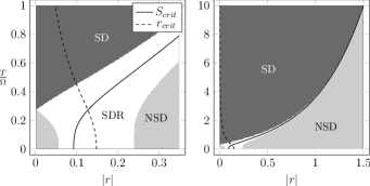
The squeezing factors $r$ and $r_{crit}$ are defined in Eq. (17), and $S_{crit}$ is given by $S_{crit}=\frac{1}{2}\log(4\Delta x_{+}\Delta p_{+}\Delta x_{-}\Delta p_{-})$. From this, it is clear that we can identify three different ‘phases’ for the asymptotic entanglement. First, if $E(t)\leq 0$ the asymptotic state is not entangled. This phase is called SD (Sudden Death). On the other hand, if $E(t)>0$ the asymptotic state is entangled. This phase is called NSD (No Sudden Death). Finally, there is an intermediate situation in which the function $E(t)$ alternates between positives and negatives values. In this case the asymptotic entanglement suffers successive events of ‘sudden death’ and ‘sudden revivals’, and so this phase is called SDR (Sudden Death and Revivals). These three phases are illustrated in Fig. 1 for the case of position coupling with an Ohmic environment. For any initial squeezing $r$, there exists a temperature above which the asymptotic state enters the SD phase, i.e., it is separable. This critical temperature grows exponentially with the initial squeezing $r$, which is a resource to create entanglement. For low temperatures a surprising result emerges (as it is non-perturbative, it is missed by perturbative treatments Vasile2010 ): There is an NSD island which is due to the fact that the asymptotic state is squeezed. For symmetric coupling the phase diagram is much simpler: Only two phases (SD and NSD) exist. In what follows we will see that the dynamics of discord shows many differences and some similarities with the above results.

IV.2 Asymptotic Gaussian discord

IV.2.1 Symmetric coupling

Figure 2: Type of measurement that minimizes the Gaussian discord of the asymptotic state. HM: homodyne measurements. HT: heterodyne measurements. Ohmic environment and symmetric coupling. $\Lambda=20$, $\gamma=0.1$, $M=1$, $\Omega=1$, $C_{12}=\tilde{C}_{12}=0$.

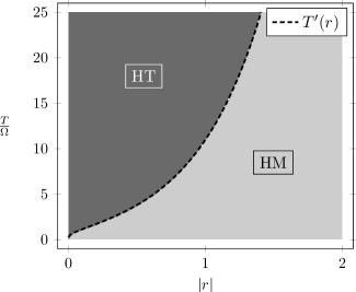
The Gaussian discord of the asymptotic state can be evaluated using Eqs. (21), (22), and (23) together with the expressions for the symplectic invariants in Eq. (15). For symmetric coupling the $+$ mode is not squeezed ($r_{crit}=0$) and all the symplectic invariants become time independent (i.e., $h(t,r,r_{crit})=\cosh(2r)$). For simplicity, we consider the non interacting case ($C_{12}=\tilde{C}_{12}=0$) and restrict ourselves to initially pure states for the moment ($\phi_{-}=1/2$). There are two interesting aspects of quantum discord in the asymptotic regime. First, we analyze what measurement optimizes the extraction of information between the two components of the system (this is needed to obtain the actual value of the discord). After that, we look at the asymptotic value of Gaussian discord as a function of squeezing and temperature.

Figure 2 shows the type of measurement, homodyne or heterodyne, that minimizes the Gaussian discord of the asymptotic state. It is clear that this phase diagram has the same topology than the one characterizing the dynamics of the entanglement in the asymptotic regime. For any given temperature, there is a degree of squeezing after which the optimal measurement is always homodyne (HM). Contrarily, heterodyne (HT) measurements are optimal for temperatures above a certain curve $T^{\prime}(r)$. This is a natural result, in fact in the limit of infinite squeezing there is an observable associated with the relative motion between the two oscillators that is perfectly localized. For example, if the observable $q_{-}=\frac{1}{\sqrt{2}}(x_{1}-x_{2})$ is perfectly localized and the position of mode $2$ is measured, then the state of mode 1 collapses to an eigenstate of $x_{1}$. This is a pure state with zero entropy. Therefore, the (homodyne) measurement of the position in mode 2 minimizes the discord since the minimum possible value of the sum of Eq. (20) is achieved. It is worth pointing out that because the asymptotic state for our system is symmetric, the discord doesn’t depend on the choice of the subsystem that is measured, as is generally the case. A simple expression for the curve $T^{\prime}(r)$ can be obtained from Eqs. (23) and (15). With $\phi_{-}=1/2$ and $r_{crit}=0$, the discriminant $g$ of eq. (23) is a polynomial of degree 8 in the variables $\phi_{+}=\frac{1}{2}\coth(\frac{\Omega}{2T})$ and $h=\cosh(2r)$. The curve $T^{\prime}(r)$ correspond to points for which $g=0$. This happens if and only if $h=h_{crit}(\phi_{+})$, with:

$$h_{crit}(\phi_{+})=\frac{-1}{3}\phi_{+}+\frac{1}{6}\sqrt{16\phi_{+}^{2}+56+\phi_{+}^{-2}}-\frac{1}{12\phi_{+}}$$ (27)

The function $T^{\prime}(r)$ is defined implicitly by $\cosh(2r)=h_{crit}(\phi_{+}(T^{\prime}))$. For high temperature or squeezing $\phi_{+}\simeq\frac{T}{\Omega}$, $h_{crit}\simeq\frac{\phi_{+}}{3}$ and $\cosh(2r)\simeq\frac{e^{2r}}{2}$. Then $T^{\prime}(r)\simeq\frac{3\Omega}{2}e^{2r}$.

Figure 3: Gaussian discord for the equilibrium state. Ohmic environment and symmetric coupling. $\Lambda=20$, $\gamma=0.1$, $M=1$, $\Omega=1$, $C_{12}=\tilde{C}_{12}=0$.

Figure 4: Gaussian discord for the equilibrium state. Ohmic environment and symmetric coupling. $\Lambda=20$, $\gamma=0.1$, $M=1$, $\Omega=1$, $C_{12}=\tilde{C}_{12}=0$.

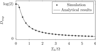
It is simple to show that discord can never disappear in a finite time (i.e., there is no sudden death of discord). Figure 3 shows the asymptotic value of the Gaussian discord as a function of the initial squeezing $r$ and the temperature $T$. As expected, for low temperatures Gaussian discord grows with the squeezing. On the other hand the temperature dependence is rather surprising: There is a temperature after that Gaussian discord grows with temperature approaching a saturation value which can be shown to be equal to $\log(2)$. This is not expected as discord is a measure of quantum correlations, which decrease with temperature. This result can be analytically found for high temperatures: Thus, in such a case the symplectic invariants are $A=B\simeq C\simeq\frac{\phi_{+}^{2}}{4}$, and $D=\phi_{+}^{2}\phi_{-}^{2}$. Then, $E_{min}\simeq 4(\phi_{-}+1/4)^{2}$ and the Gaussian discord is:

$$D_{sup}=f\left(\phi_{+}/2\right)-f\left(\phi_{+}\right)-f\left(\phi_{-}\right)+f\left(2\left(\phi_{-}+1/4\right)\right)$$ (28)

As $f\left(\phi_{+}/2\right)-f\left(\phi_{+}\right)\rightarrow-\log(2)$, for initially pure states (for which $\phi_{-}=1/2$), we have $D_{sup}=\log(2)$, as Fig. 4 indicates. This high temperature result for Gaussian discord is independent of the asymptotic squeezing of the $+$ mode. Therefore, it is also valid for the case of position coupling that will be discussed below. For high temperatures the optimal Gaussian measurement is always heterodyne and in this case the non-orthogonality of Gaussian states seem to pose a constraint on the maximal information that one can gather about one system by performing Gaussian detection on the other. It seems that this is the cause of the failure of Gaussian discord as a good approximation to true discord (which, as a measure of quantum correlations, must decrease with growing temperature in the high temperature regime).

IV.2.2 Position coupling

Figure 5: Type of measurement that minimizes the Gaussian discord for the asymptotic state. Position coupling and Ohmic environment. $\Lambda=20$, $\gamma=0.1$, $m=1$, $\Omega=1$, $C_{12}=0$.

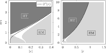
If the system-environment interaction is through position the asymptotic state is squeezed (the squeezing is measured by $r_{crit}$). As a consequence, the local symplectic invariants of the asymptotic state become time dependent (they oscillate periodically with frequency $\omega_{-}$, as seen in Eqs. (15) and (16)). The type of measurement that optimizes the extraction of information between the two subsystems changes because of this fact. This is seen in Figure 5. As opposed to the case discussed above, the phase diagram characterizing the optimal measurement shows three distinct phases. Again, large squeezing and high temperatures are, respectively, associated with HM and HT measurements. However, the fact that the asymptotic state is squeezed due to the coupling induces a low temperature phase where the optimal measurement is homodyne. The existence of an explicit time dependence in the asymptotic state reflects on the fact that the HM and HT phases are separated by a new phase where the optimal measurement depends on time (for some times the optimal measurement is homodyne while for other times such measurement is heterodyne). This is rather similar to what happens with the phase diagram characterizing the evolution of the entanglement in the long time limit. The curve $T^{\prime}(r)$ that separates the two phases for the case of symmetric coupling is plotted for reference. The new time dependent phase disappears for high temperatures (this is due to the fact that for the Ohmic environment we are considering $r_{crit}\rightarrow 0$ for increasing temperature).

Figure 6: Peak-to-peak amplitude for the oscillations of the Gaussian discord in the equilibrium state. Position coupling and Ohmic environment. $\Lambda=20$, $\gamma=0.1$, $m=1$, $\Omega=1$, $C_{12}=0$.

The asymptotic value of discord in this case is also time dependent: Gaussian discord oscillates with $\omega_{-}$ frequency. The mean value of the oscillations behaves essentially like the Gaussian discord for the symmetric coupling case (Fig. 3). Figure 6 shows the peak-to-peak amplitude $\Delta D$ of the oscillations of the Gaussian discord in the equilibrium state. Again, because $r_{crit}$ goes to zero rapidly for increasing temperature, the amplitude $\Delta D$ of the oscillations becomes negligible for temperatures that are a few times larger than $\Omega$.

IV.2.3 Mixed initial states

All the previous results were obtained for pure initial states, i.e., $\phi_{-}=1/2$. Now we explore how the results change if this condition is relaxed. For simplicity, only symmetric coupling and Ohmic environments are considered.

Figure 7: Type of measurement that minimizes the Gaussian discord for a mixed initial state with $\phi_{-}=3/2$. Symmetric coupling and Ohmic environment. $\Lambda=20$, $\gamma=0.1$, $M=1$, $\Omega=1$, $C_{12}=\tilde{C}_{12}=0$.

Figure 8: Gaussian discord of the asymptotic state versus the temperature of the environment. Mixed initial state with $\phi_{-}=3/2$. Symmetric coupling and Ohmic environment. $\Lambda=20$, $\gamma=0.1$, $M=1$, $\Omega=1$, $C_{12}=\tilde{C}_{12}=0$.

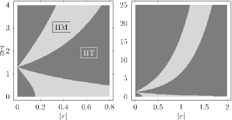
The nature of the measurement minimizing the Gaussian discord is shown in Fig. 7 for a mixed initial state with $\phi_{-}=3/2$. There are obvious differences between this and the corresponding figure for a pure initial state (see Figure 2). Some of the results are also counter intuitive: for example, in the limit of large squeezing the optimal measurement turns out to be heterodyne. The asymptotic value of discord decreases when increasing the initial mixedness. This is shown in Figure 8 where the asymptotic value of the Gaussian discord is shown as a function of the temperature for different values of the initial squeezing (for $\phi_{-}=3/2$). The asymptotic value of Gaussian discord in the high temperature limit can be analytically estimated using equation 28. Thus, the asymptotic value of Gaussian discord is examined as a function of the initial mixedness of the state (which is estimated by the effective temperature derived from $\phi_{-}$, $T_{0}$, which is such that $\phi_{-}=\frac{1}{2}\coth(\frac{\Omega}{2T_{0}})$). This is shown in Figure 9.

Figure 9: High temperature value of the Gaussian discord of the asymptotic state versus the initial temperature of the system. The analytical results (Eq. (28)) are compared to numerical simulations.

IV.3 Dynamics of Gaussian Discord

Temporal evolution of the Gaussian discord can be analyzed by a simple exact numerical solution of the dynamical equations of the covariance matrix. Results are presented below for two sets of initial conditions corresponding to separable and entangled states for the original modes.

IV.3.1 Symmetric coupling.

Figure 10: (Color online) Gaussian discord and entanglement evolution for an entangled and a separable initial state, both with initial squeezing $r=1$. Symmetric coupling and Ohmic environment at $T=0$. $\Lambda=20$, $\gamma=0.1$, $M=1$, $\Omega=1$, $C_{12}=\tilde{C}_{12}=0$.

Figure 11: (Color online) Gaussian discord and entanglement evolution for an entangled initial state with $r=1$. Symmetric coupling and Ohmic environment at $T=4\Omega$ and $T=30\Omega$. $\Lambda=20$, $\gamma=0.1$, $M=1$, $\Omega=1$, $C_{12}=\tilde{C}_{12}=0$.

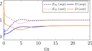
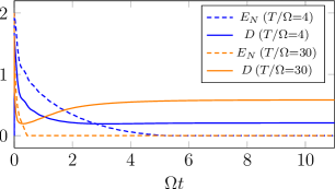
From our previous discussion it is clear that discord in the asymptotic state depends only on the initial squeezing $|r|$ of the $-$ mode. This is illustrated in Fig. 10, where it is shown that Gaussian discord behaves in the same way for both initially separable and entangled states with the same degree of squeezing ($r=1$ in this case). Three temporal scales are relevant for the evolution of quantum correlations. For example, for an initially entangled state decoherence leads to a rapid decay of both entanglement and Gaussian discord. This takes place in a timescale that is much shorter than the dynamical time of the system $\tau=2\pi/\Omega$. After this, quantum correlations oscillate with a decreasing amplitude. The timescale characterizing the oscillations is fixed by $\Omega$ while the amplitude decay is governed by $\gamma$. For the case of a $T=0$ environment, the evolution of Gaussian discord and entanglement is essentially the same. This is not true for higher temperatures, as Fig. 11 shows. As seen in the Figure, even though there is sudden death of entanglement, the Gaussian discord reaches an non-zero asymptotic value. For sub-Ohmic environments the results are similar, and the only difference is that the equilibrium state is reached faster. This is because for a sub-Ohmic environment the coupling with the low frequency oscillators in the environment is stronger.

IV.3.2 Position coupling.

Figure 12: Gaussian discord for two initial states with positive and negative squeezing. Position coupling and Ohmic environment at $T=0$. $\Lambda=20$, $\gamma=0.1$, $m=1$, $\Omega=1$, $C_{12}=0$.

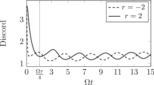
As discussed before, when system and environment interact through position, there are oscillations in the asymptotic state. The evolution of the Gaussian discord for entangled initial states is shown in Fig. 12. As before, it is seen that the mean value and amplitude of the oscillations depends only on the initial squeezing. For this case, the asymmetry between position and momentum can be seen by looking at the evolution of initial states that are squeezed either along position or along momentum. In fact, as shown in the Figure, initial states with momentum squeezing ($r<0$) are more sensitive to the environmental interaction during the initial time. Such states decohere more rapidly than states that are squeezed along position ($r>0$). For those states to decohere, dynamics has to take place (during which position and momentum exchange roles). This is clearly seen in Fig. 12. The position-momentum asymmetry is also seen in the $\pi/2$ phase difference in the long time oscillations of both entanglement and discord.

Figure 13: Gaussian discord evolution for an initial separable state with $r=1$ and different temperatures for the environment. Position coupling and Ohmic environment. $\Lambda=20$, $\gamma=0.1$, $m=1$, $\Omega=1$, $C_{12}=0$.

Figure 14: Gaussian discord and entanglement evolution for an initial state and temperature corresponding to the SDR phase ($T=0.35\Omega$ and $r=0.15$). Position coupling and Ohmic environment. $\Lambda=20$, $\gamma=0.1$, $m=1$, $\Omega=1$, $C_{12}=0$.

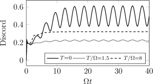
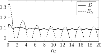
Figure 13 shows the evolution of Gaussian discord for initial separable states and different temperatures. As the temperature increases the amplitude decreases, in accordance with the results of Sec. IV.2.2. Finally, Fig. 14 compares the evolution of entanglement and Gaussian discord for an initial state and temperature corresponding to the SDR phase (see Fig. 1). It is interesting to note that the Gaussian discord attains local maximum values when the entanglement disappears.

V Conclusions

We analyzed the dynamics of Gaussian discord of a bipartite system of two harmonic oscillators that interact with a common bosonic environment. For a coupling that is bilinear (in position and momentum of both the system and the environment) the Gaussian measurement optimizing the extraction of information between the two subsystems can be obtained and used to compute the asymptotic discord. In this way, the evolution of Gaussian discord can be fully characterized in the long time limit. Finally, by means of a numerical exact solution of dynamical equations we analyzed the time dependence of discord for intermediate times (before the asymptotic state is reached). In this way, we confirmed analytical evaluation mentioned above. The results have some surprising features. Previous works on entanglement dynamics showed that such quantum correlations can be created by the interaction with the common reservoir (in fact, non-entangled initial states exhibit long time resilient entanglement). However, this is the case only for temperatures that are low enough (for any value of the initial squeezing there is a critical temperature above which the final state is separable). This is not what happens with the type of quantum correlations characterized by discord. Gaussian discord can also be created by the interaction with a common reservoir. However, once it is created by the interaction with the environment, it never disappears. As shown in our work, the asymptotic value of Gaussian discord may be small but never vanishes (as expected). The fact that the asymptotic value for Gaussian discord does not decrease (but saturates) when the temperature grows is far from intuitive. Most likely, this is an indication of the failure of the Gaussian approximation for discord in this case. True quantum discord, as a measure of quantum correlations must decrease with increasing temperature.

It is interesting to notice that our treatment enables us to obtain many exact results exploring extensively the non-perturbative, non-Ohmic and non-Markovian regimes. In fact, analytic results for entanglement in the asymptotic regime can be obtained using only the long time values of the coefficients that appear in the exact master equation. Such values are known for a variety of physically relevant cases (see Ref. Paz2009 for a collection of such results). Numerical evaluation is needed only to take care of intermediate time regimes (until the dependence on the initial state is washed out by the evolution). This treatment is in contrast with previous works, such as the one reported in Ref. Vasile2010 that make extensive use of numerical solution. In particular, using our treatment it is rather simple to relax other previous assumptions (such as the restriction to low coupling or the limitation to short time in the non-Markovian case) such as the ones used in Ref. Vasile2010 .

We gratefully acknowledge support of grants from CONICET, UBACyT and ANPCyT.

References

- [1] Harold Ollivier and Wojciech H. Zurek. Quantum Discord: A Measure of the Quantumness of Correlations. Physical Review Letters, 88(1):15–18, December 2001.
- [2] E Knill and R Laflamme. Power of one bit of quantum information. Physical Review Letters, 81(25):5672–5675, 1998.
- [3] Animesh Datta, Anil Shaji, and C.M. Caves. Quantum discord and the power of one qubit. Physical review letters, 100(5):50502, 2008.
- [4] Alireza Shabani and D.A. Lidar. Vanishing quantum discord is necessary and sufficient for completely positive maps. Physical review letters, 102(10):100402, 2009.
- [5] Vaibhav Madhok and Animesh Datta. Interpreting quantum discord through quantum state merging. Physical Review A, 83(3):032323, 2011.
- [6] D Cavalcanti, L Aolita, S Boixo, K Modi, M Piani, and A Winter. Operational interpretations of quantum discord. Physical Review A, 83(3):032324, 2011.
- [7] Bo Wang, Z.Y. Xu, Z.Q. Chen, and Mang Feng. Non-Markovian effect on the quantum discord. Physical Review A, 81(1):014101, 2010.
- [8] FF Fanchini, T. Werlang, CA Brasil, LGE Arruda, and AO Caldeira. Non-Markovian dynamics of quantum discord. Physical Review A, 81(5):052107, 2010.
- [9] T. Werlang, S. Souza, F. F. Fanchini, and C. J. Villas Boas. Robustness of quantum discord to sudden death. Physical Review A, 80(2):024103, August 2009.
- [10] Gerardo Adesso and Animesh Datta. Quantum versus classical correlations in Gaussian states. Physical review letters, 105(3):30501, 2010.
- [11] Paolo Giorda and M.G.A. Paris. Gaussian quantum discord. Physical review letters, 105(2):20503, 2010.
- [12] J.P. Paz and A.J. Roncaglia. Dynamical phases for the evolution of the entanglement between two oscillators coupled to the same environment. Physical Review A, 79(3):032102, 2009.
- [13] J.P. Paz and A.J. Roncaglia. Dynamics of the entanglement between two oscillators in the same environment. Physical review letters, 100(22):220401, 2008.
- [14] Ruggero Vasile, Paolo Giorda, Stefano Olivares, Matteo Paris, and Sabrina Maniscalco. Nonclassical correlations in non-Markovian continuous-variable systems. Physical Review A, 82(1):012313, July 2010.
- [15] Bei Lok Hu, Juan Pablo Paz, and Yuhong Zhang. Quantum Brownian Motion in a general environment. Physical Review D, 45(1):2843, 1992.