Atlasing of Assembly Landscapes using Distance Geometry and Graph Rigidity
Abstract
This paper describes a novel geometric methodology for analyzing free-energy and kinetics of assembly driven by short-range pair-potentials in an implicit solvent, and provides a proof-of-concept illustration of its unique capabilities.
An atlas is a labeled partition of the assembly landscape into a roadmap of maximal, contiguous, nearly-equipotential-energy conformational regions or macrostates, together with their neighborhood relationships. The new methodology decouples the roadmap generation from sampling and produces: (1) a query-able atlas of local potential energy minima, their basin structure, energy barriers, and neighboring basins; (2) paths between a specified pair of basins, each path being a sequence of conformational regions or macrostates below a desired energy threshold; and (3) approximations of relative path lengths, basin volumes (configurational entropy), and path probabilities.
Results demonstrating the core algorithm’s capabilities and high computational efficiency have been generated by a resource-light, curated opensource software implementation EASAL [1] (Efficient Atlasing and Search of Assembly Landscapes, see software [2], video [3] and user guide [4]). Running on a laptop with Intel(R) Core(TM) i7-7700 @ 3.60GHz CPU with 16GB of RAM, EASAL atlases several hundred thousand conformational regions or macrostates in minutes using a single compute core. Subsequent path and basin computations each take seconds. A parallelized EASAL version running on the same laptop with 4 cores gives a 3X speedup for atlas generation.
The core algorithm’s correctness, time complexity, and efficiency-accuracy tradeoffs are formally guaranteed using modern distance geometry, geometric constraint systems and combinatorial rigidity.
The methodology further links the shape of the input assembling units to a type of intuitive and query-able bar-code of the output atlas, which in turn determine stable assembled structures and kinetics. This succinct input-output relationship facilitates reverse analysis, and control towards design.
A novel feature that is crucial to both the high sampling efficiency and decoupling of roadmap generation from sampling is a recently-developed theory of convex Cayley (distance-based) custom parametrizations specific to assembly, as opposed to folding. Representing microstates with macrostate-specific Cayley parameters, to generate microstate samples, avoids gradient-descent search used by all prevailing methods. Further, these parametrizations convexify conformational regions or macrostates. This ratchets up sampling efficiency, significantly reducing number of repeated and discarded samples.
These features of the new stand-alone methodology can also be used to complement the strengths of prevailing methodologies including Molecular Dynamics, Monte Carlo, and Fast Fourier Transform based methods.
1 Introduction
This paper describes a new geometric methodology for efficient atlasing and search of assembly energy landscapes. Since many novel concepts are required to even informally describe the new methodology, the reader is referred to the Table 1.1 in Section 1.1. The table also includes a rough correspondence between new and established concepts. Formal definitions can be found in Section 3. Assembly is defined broadly as starting from tethered or flexibly bonded rigid molecular components, and driven by short-range potentials between atom-pairs in distinct components in an implicit solvent (subsuming hard-sphere or sticky-sphere models).
A key concept central to the new methodology is the atlas which is a partition of the assembly landscape into macrostates, organized as a roadmap. Each macrostate is a maximal, contiguous, nearly-equipotential-energy conformational region. Note: We refer to molecular configurations or microstates and as being conformations of each other (in the same macrostate) if their potential energies are similar and any continuous path between them does not have to cross significant energy barriers, where ‘similar’ and ‘significant’ depend on the context, and the level of discretization of the pair potentials (see Section 3.1). Otherwise, they are in different macrostates. The atlas further stratifies macrostates by energy level.
The methodology provides resource-light, stand-alone algorithms that can also be used to complement prevailing general ones such as Monte Carlo and Molecular Dynamics, as well as specialized ones used in docking. The unique features are:
-
1.
mitigating the curse of dimension in configurational entropy (free energy) and kinetics computations by
-
(a)
decoupling exploration from sampling, i.e., generating an atlas of the landscape - including basins, barriers, paths and their neighborhood relationships - with minimal sampling, using geometric constraints [5] and rigidity-based roadmap;
-
(b)
convexifying macrostates using customized, Cayley parametrization[6], which is a distance-based internal coordinate representation of assembly configurations that are constrained by inter-atomic distances (formally defined in Section 3.4); this parametrization achieves high sampling efficiency and accuracy, avoiding gradient-descent, and repeated or discarded samples;
-
(a)
-
2.
formally isolating succinct topological and geometric characteristics - intuitive bar-codes - that differentiate assembly landscapes from each other;
-
3.
exploiting characteristics that differentiate assembly landscapes from more complex folding landscapes;
-
4.
establishing a connection between these succinct bar-codes and the geometry of the input assembling structures, e.g., to facilitate labeling, querying, reverse analysis and design of landscapes;
-
5.
mathematically proving efficiency and accuracy guarantees.
The emphasis of this paper is not formal comparisons with prevailing methodologies, nor demonstration of performance on benchmarks [7, 8] for macromolecular or spherical cluster assembly systems (see Section 2.5 for a discussion on companion papers). Rather, the emphasis here is on describing the new methodology and core algorithms’ rigorous geometric underpinnings, providing both proofs of efficiency and accuracy, and proof-of-concept results demonstrating its efficiency and unique features. The results have been generated using an opensource software implementation EASAL (Efficient Atlasing and Search of Assembly Landscapes) of the core algorithms (see software [2], video [3] and user guide [4]).
The roadmap component of the atlas is refinable, and query-able with unique, intuitive “street signs” or macrostate labels, each of which is a graph or network of geometric constraints [5], called the active constraint graph. These constraints are imposed by the short-range pair potentials that are active in that macrostate, i.e., each constraint is between an atom-pair whose inter-atomic distance achieves minimum energy, treated in the limit as a hard-sphere potential. Thus a macrostate is an active constraint region whose effective dimension can be determined using combinatorial rigidity [5] of the active constraint graph. Consequently, the effective dimension becomes a proxy for the energy level of the macrostate. The theory presented here extends easily to longer range potentials with a slight modification to the way the potentials are geometrized, as explained in detail in Section 3.1. However, for ease of exposition, we use short-range potentials throughout the paper.
Microstates or configurations, which are traditionally represented using Cartesian parameters, are instead represented using Cayley or distance-based parameters that are customized to the active constraint graph of the macrostates. As we show in Section 3.4, generating microstate samples within an active constraint region using Cayley parameters avoids gradient-descent search used by all prevailing methods to sample constrained regions. Further, under Cayley parametrizations, active constraint regions or macrostates become convex with easily computable bounds.
We show that the convexification technique applies readily to macrostates in assembly, but not so readily to folding. In a convexifiable macrostate or active constraint region, there is a collection of atom pairs (the Cayley parameters , which are not active constraints) satisfying the following property: between any pair of configurations or microstates there is a path in the macrostate along which the inter-atomic distances maintain a linear or affine relationship. Thus, very roughly speaking, an assembly system can follow straight paths, in a certain formal sense, and still avoid breaking energy barriers, i.e., while remaining in the same macrostate (a contiguous, nearly equipotential energy region). However, a folding system, lacking convexifiable macrostates, may be forced to follow a convoluted path in order to remain in a macrostate.
Convexification improves sampling efficiency for assembly landscapes, significantly reducing the number of repeated and discarded samples. Overall, the methodology directly addresses the curse of dimension and complexity of landscapes while giving formal guarantees of efficiency, accuracy, robustness and tradeoffs for the core algorithms (see Section 4.5).
Furthermore, the methodology isolates input shape variables of the assembling units that directly influence landscape design variables, including the number of macrostates and the average Cayley parameter value. The values of the design variables yield a succinct bar-code for the output atlas.
Finally, a single-threaded software implementation of the core algorithms, EASAL [1] (see software [2], video [3] and user guide [4]), atlases several thousand (resp. hundred thousand) macrostates and computes entropy integrals of reasonable accuracy in minutes (resp. a couple of hours) on a laptop with Intel(R) Core(TM) i7-7700 @ 3.60GHz CPU with 16GB of RAM, running on a single core, for bi-assemblies of up to 42-atom alpha-helices, and for clusters of up to 24 identical sticky-sphere particles. Subsequent path computations each take seconds. A recent proof-of-concept parallelized EASAL version running on the same laptop, with 4 cores, gives a 3X speedup in preliminary tests. Efficiency can improve significantly when the assembling entities are identical, by exploiting symmetries in the landscape [9]. Although the proof of concepts results demonstrated in this paper only sample bi-assemblies of up to 42-atom alpha-helices, EASAL is more generally applicable to other bi-assemblies of rigid molecular components of much larger size. EASAL has been used to analyze assemblies of rigid molecular components with atoms [10, 11].
1.1 Basic Concepts and Terminology
The following table gives the list of terms and their definitions used in this paper.
| active constraint | A pair of atoms from different rigid molecular components satisfying constraint of the assembly problem (formally described in Section 3.1). |
| assembly problem | Problem (, ) for general (formally described in Section 3.1.2). |
| rigid molecular component, , | The set of atom centers in a rigid molecule. rigid molecular components are inputs to the assembly problem (formally described in Section 3.1.2). |
| assembly landscape | Complete set of solution configurations of the assembly problem (formally described in Section 3.1.2). |
| macrostate | Maximal, contiguous, nearly-equipotential-energy conformational region. |
| microstate | A molecular configuration. |
| dimension of assembly landscape | Dimension of the assembly landscape (formally described in Section 3.1.2). |
| ambient dimension | Ambient dimension of assembly problem (formally described in Section 3.1.2). |
| roadmap | A directed acyclic graph whose nodes are active constraint regions. Edges go from parent to child active constraint regions (formally described in Section 3.2). |
| stratification | Organization of the roadmap by dimension, i.e., energy level (formally described in Section 3.2). |
| active constraint region | A finite set of maximal, contiguous, nearly equi-potential energy regions (macrostates) that have the same set of active constraints (formally described in Section 3.2). |
| active constraint graph | The vertices are the atoms involved in active constraints, plus at least 3 atoms from each of participating rigid molecular component. Two types of edges: (1) pairs that are active constraints and (2) all pairs such that both belong to the same rigid molecular component(formally described in Section 3.2). |
| parent region in roadmap | Higher dimensional, higher energy level, interior active constraint regions (formally described in Section 3.3). |
| child region in roadmap | 1 lower dimensional (compared to parent), lower energy level, boundary active constraint regions (formally described in Section 3.3). |
| atlas | A topological roadmap of the assembly landscape (formally described in Section 3.4.1). |
| Cayley parameters | Non-edges in the active constraint graph that make it a 3-tree (formally described in Section 3.4.1). |
| Cayley configuration | A tuple of realizable length values of Cayley parameters for an active constraint graph (formally described in Section 3.4.1). |
| Cayley region | The complete set of Cayley configurations in an active constraint region (formally described in Section 3.4.1). |
| chart | The parameter map taking the (sampled) Cartesian configurations in an active constraint region to the corresponding Cayley configurations (formally described in Section 3.4.1). |
| input shape variables | The two variables width and concavity that describe the input rigid molecular components (formally described in Section 3.5). |
| landscape design variables | The variables used to facilitate control towards the design of the landscape (formally described in Section 3.5). |
| witness | The first configuration discovered in a region from the parent region, in which a new active constraint becomes active (formally described in Section 3.6.1). |
Organization
The next Section 2 describes related work and delineates the contributions of this paper. The Methods Section 3 formally describes the new methodology’s distinct features and strategies - sketched in the introduction - for generating (desired portions of) the atlas. The Results Section 4 provides proof of concept illustrations of the methodology’s unique capabilities, using the EASAL software implementation [1, 3, 2], including verification of the theoretical efficiency and accuracy. These should be considered starting points for the results and comparisons in the companion papers and future work (see Section 2.5, and Section 5).
2 Related Work and Contributions
Throughout this paper, we use two variables to differentiate between basic types of assembly systems: and respectively denote the number of assembling rigid molecular components (e.g. helices, clusters), and the maximum number of points (e.g. atoms/particles) in any of them. The rigid molecular components are assumed to be flexibly tethered or bonded to each other, with the assembly being driven by weak interactions modeled as short-range, Lennard-Jones pair potentials, in an implicit solvent.
We do not review the extensive literature on (ab-initio) simulation or decomposition-based methods that are required to tractably deal with large assemblies with , such as viral capsids. Direct computations of free energy, binding affinity and kinetics of assembly are challenging even starting from much fewer rigid molecular components. The challenges discussed below are due to high dimensionality as well as topological and geometric complexity of the potential energy landscape.
2.1 Exploiting Assembly Landscapes
The simplest form of molecular assembly is site-specific docking, where a small molecule initially in solution (the ligand) binds to a specific site in a much larger molecule (the receptor). Diverse methods from computational geometry, vision and image analysis have been used in site-specific docking algorithms [12, 13, 14, 15, 16, 17, 18, 19]. Unlike the more general goals of the new methodology itemized earlier, the goal of these algorithms is to find site-specific docking configurations or microstates with optimal binding affinity. While this depends on equilibrium free energy as well as kinetics between stable states, docking methods arbitrarily restrict the region of possible configurations or microstates to evaluate an approximate free energy function. On the other hand, prevailing methods for more general free energy and kinetics computation must incorporate both the depth and relative weighted volumes (entropy) of basins and their topological relationships . These use highly general approaches such as Monte Carlo (MC) and Molecular Dynamics (MD) simulation.[20, 21, 22, 23, 24, 25, 26, 27, 28, 29, 30, 31, 32, 33, 34, 35]
There exist a number of methods to explore the volume or configurational entropy of the free energy basin landscape using the fact that effective dimension of macrostates is a proxy for energy level. Small cluster assemblies from spheres [36, 37, 38, 39, 40, 41, 42], i.e., and arbitrary, ( is typically without decomposition), are used in the study of mesoscale systems such as molecule [43, 44], cDNA strands [45] and colloids interacting via depletion [46]. These can be modeled as a short-ranged potentials particle system in which the interaction length is much smaller than the system size. That is, their Lennard-Jones wells are narrow and they can be treated as a Hard Sphere assembly systems. For these systems, there exist a number of methods to compute paths and kinetics as well as free energy and configurational entropy of lower dimensional or lower energy macrostates [47, 36, 37, 38, 39, 40, 41, 42]. Newer methods study the change in the energy landscape of spherical particles when the interaction potentials change from a Lennard-Jones type potential to sticky hard-sphere type potential [48, 49]. Taken together, these methods output trajectories of sample configurations from free energy landscapes of a wide variety of systems.
However, these prevailing methods do not explicitly take advantage of the relative simplicity of constraint systems that drive assembly compared to folding. As we explain in detail in Section 3.4, constraint graphs that arise in assembly yield convexifiable configurational regions whereas a folding system has dense cycles of constraints that prevent convexification. Although the energy and force models used by MC and MD differ implicitly in assembly and folding, these methods miss out on critical advantages by not explicitly exploiting special geometric properties of small assembly configurational regions. In contrast, the new methodology specifically exploits assembly constraint graph properties via Cayley convexification[6].
2.2 Decoupling Roadmap generation from Sampling
Larger assemblies are dimensionally intractable without recursively decomposing into smaller ones [10]. Recombining requires estimating not only the equilibrium free energy but also the kinetics for each smaller intermediate assembly. Understanding kinetics requires a topological roadmap of potential energy basins, i.e., the neighborhood and boundary relationships of macrostates, especially when they feed into multiple basins.
Yet, most prevailing methods either do not extract a comprehensive topological roadmap even for small assemblies, or do so in conjunction with extensive sampling for configurational entropy or free energy computation. Decoupling roadmap generation, i.e., topology extraction, from sampling is one of the key achievements of the new methodology.
Ergodicity of methods such as MC and MD is unproven for configurational regions of high geometric or topological complexity with low energy regions or macrostates of low relative volume (low effective dimension) separated by high energy barriers. Hence they require unpredictably long trajectories starting from many different initial configurations or microstates for locating such separated regions or macrostates. Starting from MC and MD trajectories, recent heuristic methods infer a topological roadmap [50, 51, 52, 53] and use topology to guide dimensionality reduction [54]. Methods for handling broken ergodicity include basin-hopping [55] (an optimization technique to find global minima), and the use of parallelism [56] or some combination of the two [57, 58]. All of these methods are extremely resource intensive and rely on heavy sampling.
A version of assembly arises in the robotics motion planning literature with exponential time algorithms to compute a roadmap (a version of atlas) and paths in general semi-algebraic sets [59, 60, 61], with probabilistic versions to improve efficiency [62, 63]. For the Cartesian configurational regions of non intersecting spheres, the works [64, 65] characterize the complete homology, viable only for relatively small point-sets or spheres, while more empirical computational approaches for larger sets [66, 67] come without formal algorithmic guarantees. A geometric rigidity approach was primarily used to characterize the graph of contacts of arbitrarily large jammed sphere configurations in a bounded region [68, 69].
Unlike the above approaches, the new methodology gives a comprehensive atlas of the assembly macrostates as fast as possible, by using macrostate-specific, so-called, Cayley parametrization to decouple sampling from exploration of landscape topology. In addition, unlike many former approaches, our methodology is deterministic, its efficiency following from exploiting special properties of those semi-algebraic sets that arise in assembly.
While the work[70] also uses the word ‘atlas’ and refers to a configurational region stitched together from custom-sampled subregions called ‘charts’, both the decomposition into subregions and the definition of charts are entirely unrelated to our methodology. That work uses neither active constraint regions, nor stratification by energy levels, nor Cayley parameters for convexification and does not focus on assembly but systems such as cyclo-octane, where loop-closure type constraints predominate. The paper [47] uses a partition into active constraint regions that they call ‘modes’. They compute minimum potential energy states and kinetics using certain integrals over low dimensional macrostates of the interacting particles.
The paper [47] formally showed that their (and our methodology’s) geometrization of such systems is physically realistic. However, they directly search for hard-to-find minimum energy macrostates (effectively zero dimensional) by walking one-dimensional macrostates. In contrast, our methodology uses the dimensional stratification in the atlas: it starts from Cayley convexified higher-dimensional interior (parent region) and recursively locates easy-to-find boundary macrostates of exactly one less effective dimension.
2.3 Designing Landscapes
The prevailing methods described above are not particularly suited to reverse analysis. By reverse analysis we mean: isolating and altering features of the output landscape and free energy by tweaking input shape variables of the assembly constituents and interactions. Our methodology links the shape of the input assembling units to a type of intuitive and query-able bar-code of the output atlas, such as the number of active constraint regions or macrostates and their average Cayley parameter values. These landscape design variables can be used to design stable assembled structures and kinetics. This succinct input-output relationship facilitates reverse analysis, and control towards design.
2.4 Sampling and Computing Entropy Integrals
While the computation of potential energy of a given configuration is generally straightforward, free energy computation requires accurate entropy computation, i.e., relative (weighted) volume of potential energy basins, each of which is a complicated mosaic of macrostates of varying effective dimension. Similarly, kinetics requires the computation of path probabilities. As mentioned in Section 2.1 prevailing methods use exhaustive sampling for path and volume computations. For , there are bounds for approximate configurational entropy using robotics-based methods without relying on MC or MD sampling [31].
For small cluster assemblies from spheres, there exist a number of methods to compute free energy and configurational entropy of lower dimensional or lower energy macrostates [47, 36, 37, 38, 39, 40, 41, 42, 71].
However, working with Cartesian configurations as microstates, they must deal with macrostates that are comparable in topological complexity to the entire Cartesian configurational region of small molecules such as cyclo-octane [72, 70, 73].
In general, lower energy macrostates are probabilisitcally weighted higher, but have lower effective dimension which - in principle - should make sampling faster since time complexity of the volume integral computation (via sampling) is exponential in the effective dimension of the macrostate. However, such macrostates - which live within a much higher ambient dimension - are typically topologically complex. Ambient dimension is the maximum dimension of any macrostate in the assembly configuration space, specifically a region with no active constraints (discussed in Section 3.1.2). Staying within such an effectively lower dimensional macrostate, a nearly constant potential energy region, confounds most prevailing methods, forcing them to rely on local linearization and energy gradient descent (to enforce the energy constraints) leading to many discarded samples. For example the paper [47] needs to solve a non-linear equation iteratively when tracing a 1 or 2-dimensional constrained manifold by moving a Cartesian configuration along its tangential direction and projecting it back to the manifold.
Stratified sampling [74]could be considered a general way to address this problem by using stratified probability distributions whose support is restricted to a constant potential energy region. However, membership of a configuration in a region is characterized by the tangent space (linearization using Eigen vectors) at that particular configuration. Hence, the configuration needs to be sampled first, which does not address the original difficulty of staying primarily within the bounds of the desired region, i.e., computing the bounds of the support of the probability distribution. In general, while the above-mentioned methods address the accuracy issue in sampling effectively low dimensional regions, they do so at the expense of many discarded samples and efficiency.
The new methodology addresses both the accuracy and efficiency issues via a region-specific Cayley convexification ensuring that sampling (for volume computation) stays within macrostates without having to explicitly enforce any constraints. For a given Cayley configuration sample, our methodology computes the Cartesian configurations directly via evaluation, minimizing discarded and repeated samples. Specifically, instead of sampling in the Cartesian region which limits most methods, Cayley sampling permits our methodology to sample macrostates of any dimension.
On the other hand, higher energy regions or macrostates are effectively higher dimensional; hence their volume computation by sampling is tractable only when the number of rigid assembly constituents is small since the dimension of the ambient space is exponential in . For such higher dimensional regions or macrostates, the new methodology does not have to rely entirely on sampling, but utilizes the convexity arising from Cayley parametrization.
Finally, using fast, flexible sampling options [75], our methodology helps to rapidly find paths and compute entropy integrals through multiple regions or macrostates of various energy levels or effective dimensions, enabling kinetics computation.
2.5 Delineating Contributions of Directly Related Work
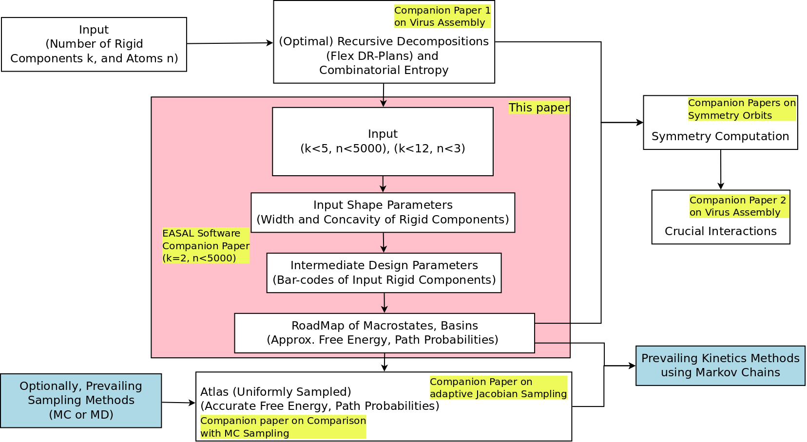
Figure 1 shows the original contributions of this paper and its connections with prevailing methods as well as companion papers whose contents are sketched below. (1) A conference proceedings paper that provides an early sketch of some aspects of the new methodology prior to the EASAL software implementation. This paper does not contain results. (2) A multi-perspective comparison of algorithmic variants of the new methodology against metropolis Monte Carlo (MC) sampling for the assembly landscape of 2 transmembrane helices, in order to assess complementary strengths [76]. (3) Using an adaptive Jacobian strategy along with convex Cayley parametrization for high-performance sampling towards entropy integral computation [75]. (4) Prediction of assembly-crucial inter-monomer-interface interactions with experimental mutagenesis validation for 3 viral capsids [10, 11] (Minute Virus of Mice (MVM), Adeno-Associated Virus (AAV), and Bromo-Mosaic Virus (BMV)) - utilizing the recursive decomposition (reverse assembly pathway) of the large viral capsid assembly into smaller assembly intermediates [77, 78], (5) Exploitation of symmetries [9]. (6) Curated opensource software and a user-developer manual that provides a summary of all of the above, as well as a paper describing the software implementation, clearly citing and summarizing the above papers as well as this manuscript [1].
Note: For ease of exposition, we use “active constraint regions” and “configurations” respectively to refer to macrostates and microstates. Technically, these have different meanings when expressed in Cartesian and Cayley parameters. Moreover, active constraint regions may not be contiguous, while macrostates are. However, as shown in Sections 3.4.1 and 3.4.2, our use of Cayley parametrization ensures that this ambiguity is not an issue when the context is clear.
3 Methods
The new methodology uses several key strategies to generate the assembly configurational regions. Section 3.1 discusses geometrization of short-range Lennard-Jones potentials as active geometric constraints, by which effective dimensions of active constraint regions become proxies for energy levels. Section 3.2 introduces a dimensional classification of active constraint regions, called Thom-Whitney stratification, using active constraint graphs.
In Section 3.3 we describe a recursive method that along with stratification decouples the generation of the roadmap from sampling. In Section 3.4 we describe how to find a lower dimensional boundary of a given region, using a a distance based region-specific Cayley parametrization to convexify the region.
In Section 3.5 we establish a connection between the input molecular geometry and the output features (a type of bar-code of the output) via landscape design variables.
Section 3.6.1 sketches the core algorithm for 2 input rigid molecular components (, arbitrary). This is followed by algorithmic variants for multimers (, arbitrary) in Section 3.6.4 and for cluster assembly from spherical particles (, ), with improvements when the assembling components are identical in Section 3.6.5; and we briefly describe under what conditions and how the approach can be extended to the general case ( arbitrary, arbitrary) in Section 3.6.6.
In Section 3.7 we discuss algorithmic extensions
to compute basins, barriers, paths, and volumes.
Note: most of the illustrative figures in this section are generated by the EASAL implementation of the new methodology [2, 1, 3].
3.1 Geometrization and Input Setup
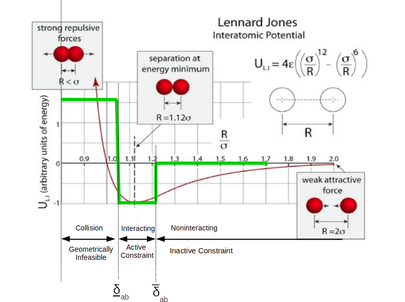
With , the distance between the centers of atoms and , we geometrize the inter-atomic short-range Lennard-Jones potential energy terms into 3 main regions (see Figure 2):
-
i
Large distances at which nearly zero force is exerted between the atoms, such atom pairs, called inactive constraints, correspond to atom pairs such that , .
-
ii
Very close distances that are prohibited by inter-atomic repulsion or inter-atomic collisions, corresponding to pairs such that , .
-
iii
The interval between these, known as the short-range Lennard-Jones well, in which bonds are formed. Atom pairs in the well are called active constraints and corresponding to the preferred distance .
| (1) |
The steric or collision distance keeps atom-centers apart; is the distance beyond which the Van der Waals forces are no longer relevant. The interval is called the well. When , is a Hard-Sphere potential. The function is discretized (see Equation 1) so that is constant.
Note: For longer range potentials, the LJ well can be discretized
into several intervals according to the energy level. Assuming that the well
has levels, the active constraint region with one constraint will have
sub-regions. Each sub-region will have constant energy. A region with
active constraints will have such sub-regions. For ease of
exposition, we use in the rest of the paper.
The assembly problem can now be viewed as exploring the feasible relative positions of a collection of point sets, each of size , in that are mutually constrained by distance intervals. Here, each point set corresponds to a rigid molecular component such as helices, each point in the point set corresponds to the center of an atom and the distance constraints correspond to the discretized short-range Lennard-Jones potentials.
3.1.1 Geometrization Example Toy
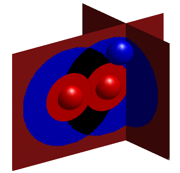
To concretely illustrate the notion of geometrization, consider an input system consisting of two rigid molecular components: consists of two atoms and with centers at a fixed distance ; is a single atom with center (see Figure 3). The atom steric radii are 1/2, i.e, the center of must maintain a distance of at least 1 from the centers of and . The potential energy of this system is the sum of the short-range Lennard Jones potentials: .
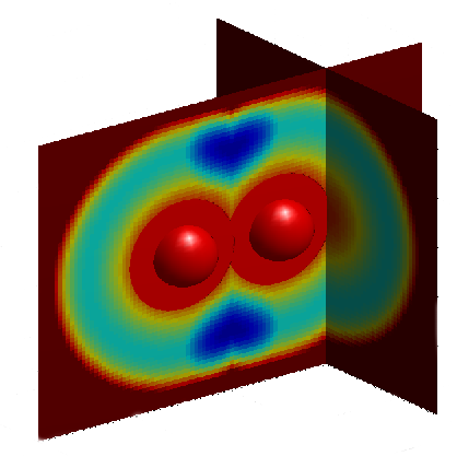
Since the energy is invariant under Euclidean rigid transformations, we may fix and . Figure 3 illustrates the discrete () geometrization of the energy landscape. The lower short-range Lennard-Jones bound prevents from falling into the red region surrounding the red atoms and . Similarly does not interact with and when its center is in the outer burgundy region corresponding to inactive configurations. The lowest energy is obtained when lies in the well of both and and two constraints are active. The lowest state corresponds to a black torus whose two transversal 4-sided sections are shown on the front-facing slice. The torus is formed as the intersection of the effectively 2-dimensional blue spherical shells of the two energy wells. Figure 3 uses a finer discrete geometrization with large .
3.1.2 Assembly Problem, Input and Output
With this setup, the core method takes as input an assembly system which consists of up to four items.
-
1.
A collection of rigid molecular components with atoms each. In the context of molecular assembly, each , , is specified as the positions of at most atom-centers.
-
2.
Distance interval constraints on point pairs given by .
- 3.
-
4.
Optional: set of active constraint regions of interest, specified by their active constraint graphs.
Consider two rigid molecular components and , of size , in , that are mutually constrained by distance intervals. For atoms and , define as , where is a Euclidean orientation preserving isometry, and is the special Euclidean group in . is feasible if the following hold:
| () | |||||
| () |
Constraint implies that is infeasible when there exists a pair that is too close. Constraint implies that at least one pair is within a preferred distance interval. When is feasible, the Cartesian configuration is called a realization of the constraint system (, ). Assembly problem (, ) asks for a description of the realization space or the Cartesian configurational region of feasible ’s. This is the assembly landscape .
When , the ambient dimension of Assembly Problem (, )
is 6, namely, the dimension of . In general is , where is
the number of rigid molecular components. When the effective
dimension of the assembly landscape is .
Note: Generally, when we refer to the assembly problem, we mean assembly problems with small assembly systems as input ( large and small, or small and large). When the input system has large and large , we get a folding system. Thus, in this paper we look at assembly and folding as all encompassed within the various ranges of and .
We make this distinction to highlight the fact that when both and are large, the active constraint graphs could be complicated enough to not permit Cayley convexification. The core algorithm in Section 3.6.1 and its variants in Section 3.6.4 and Section 3.6.5, directly atlas small assembly systems, leveraging Cayley convexification. The algorithm variant in Section 3.6.6 decomposes the larger system in a folding problem using the so-called DR-plans to take advantage of Cayley convexification.
The main output of the methodology is the topological, dimensional, and
geometric structure of the assembly landscape i.e., the set of
all feasible satisfying (, ). This is specified
as a roadmap which includes a stratification of active constraint regions by
dimension or energy levels, and their neighborhood relationships.
Each active constraint region is labeled by its active constraint graph and
comes with its Cayley and Cartesian configurations.
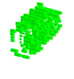
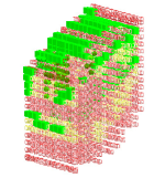
The set of Cartesian configurations is visualized as the sweep (see
Figure 4). The sweep shows one of the rigid molecular components
together with all feasible Cartesian configurations of
traced out.
Note: although Assembly Problem (, ) is defined for rigid molecular components, Sections 3.6.4, 3.6.5, and 3.6.6 show how it generalizes to arbitrary . Furthermore, the exposition of this paper assumes the case where radii , are assigned to atoms and respectively, and the constants and in (, ) (generalized to arbitrary ) are functions of .
3.2 Stratified Roadmap
We partition the assembly landscape into active constraint regions (nearly-equipotential-energy regions or macrostates).
Definition 3.1
For a configuration in the assembly landscape , i.e., a feasible configuration for Assembly Problem (, ), the vertices of an active constraint graph are the atoms involved in active constraints (atom pairs satisfying ), but additionally include at least 3 atoms from each of and . The two types of edges are (1) pairs that are active constraints for and (2) all pairs and where and (see Figure 4. An active constraint region is the set of all configurations with the same active constraint graph .
The active constraint regions are organized as a partial order (directed acyclic graph or DAG) that captures their boundary relationships (see Figure 4 and Figure 4). A node of the DAG is an active constraint region, and a directed edge captures a boundary relationship. In particular, the active constraint graph of a region is a subgraph of the active constraint graph of its children boundary regions.
More active constraints correspond to lower potential energy and the lowest potential energy is attained at the bottoms of the potential energy basins (discussed in detail, later in this section). The DAG is thus a refinable topological roadmap with unique “street signs” or region labels, which are the active constraint graphs.
In addition to indicating a boundary relationship, the DAG edges between two nodes in the roadmap indicate a dimensional relationship (see Figure 4): a lower dimensional child region is the boundary of a parent region one dimension higher (one fewer active constraint). Next we describe how the roadmap is organized into dimensional strata.
3.2.1 Generic Rigidity-based Stratification of Active Constraint Regions
Active constraint graphs are analyzed using combinatorial rigidity theory (discussed in Section A of the Appendix) [5, 82].
In particular, generically, the sum of the dimension of the active constraint region and the number of edges in its active constraint graph is the ambient dimension , which is , where is the number of rigid molecular components (see Section 3.2.2). Since the active constraint regions satisfy distance constraints which are quadratic polynomial equations and inequalities, the assembly landscape is a semi-algebraic set (a union of sets defined by polynomial inequalities). This permits a so-called Thom-Whitney stratification [83].
A Thom-Whitney stratification of an assembly landscape is a partition into active constraint regions that are grouped into strata by their dimension (see Figure 4). where the number of active constraint edges in is . For all , is effectively -dimensional, i.e., it has dimension when all its active constraints are treated as Hard-Sphere wells of zero width.
3.2.2 Genericity Assumption
In the above discussion, we assumed that generically the effective dimension of an active constraint region plus the number of active constraints is the ambient dimension , i.e., the number of active constraints is generically the co-dimension of the region. This is justified because, in Assembly Problem (, ), generically, the active constraint edges are not implied by (dependent on) the rest of the active constraint graph. In other words, implied distances are not active constraints, and inactive constraints (implied or not) do not restrict the dimension of active constraint regions. For the special case of Assembly Problem (, ), in which sets and are centers of non intersecting spheres of generic distinct radii, these assumptions are an unproven conjecture, for which counterexamples haven’t been encountered. For this conjecture has been proven [84]. When the radii are all the same, several simple counterexamples (e.g., crystalline structures with high coordination number) exist where active constraints are implied by other active constraints.
Non-generically, there could be active constraints regions of effective dimension whose number of active constraints exceeds , i.e., the active constraint system is over constrained, or some of whose active constraints are dependent. For entropy calculations, such regions should be explicitly tracked since although dependent constraints do not alter the effective dimension, they can diminish the set of configurations. For simplicity, our exposition ignores such over-constrained regions in the stratification and assumes that all regions of effective dimension are obtained by choosing exactly active constraints, i.e., they are assumed to be independent.
3.2.3 Stratification Example Toy1
To illustrate the concept of stratification further, consider Assembly Problem (, ) in with two rigid molecular components and ; contains two atoms - and - and contains two atoms - and . The ambient space is of dimension 3. A complete stratification of the Cartesian region is shown in Figure 5. The three strata are organized as a DAG, with nodes representing active constraint regions and labeled by their corresponding active constraint graphs. In , the minimum number of atoms required from each rigid molecular component in Definition 3.1 is 2 instead of 3. As in Definition 3.1, the vertices in the active constraint graph are atoms participating in the active constraints that define . The edges are of two types, (i) between atoms in the same rigid molecular component and (ii) the active constraints, between atoms in different rigid molecular components.
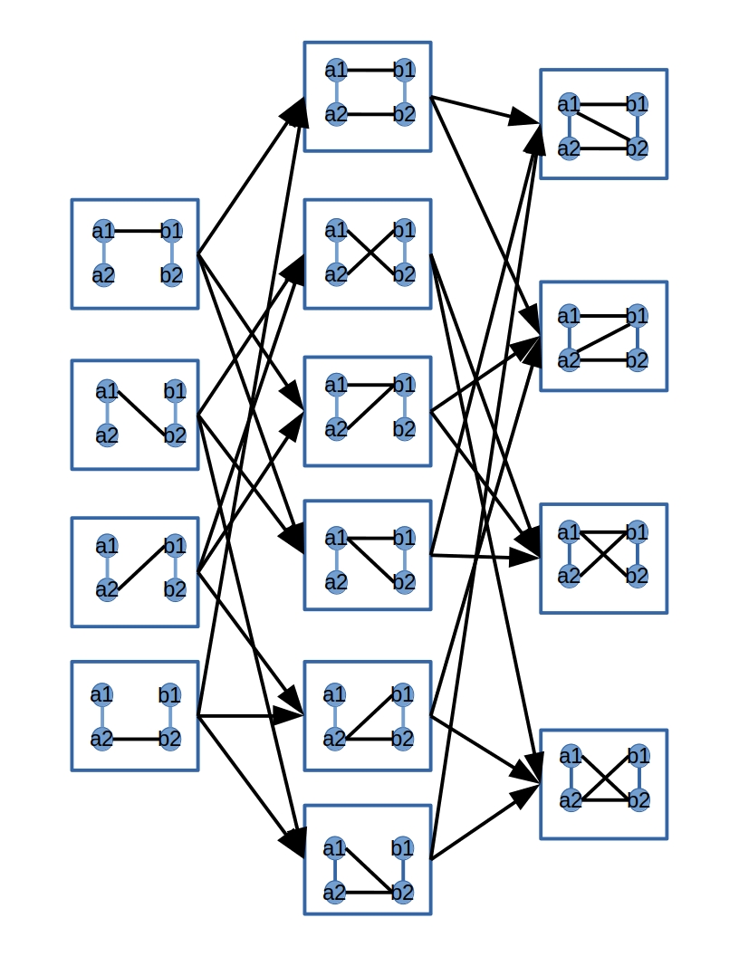
The stratum consists of the 4 regions in the left column, which are 2D regions, each containing configurations with 2 degrees of freedom. Adding an extra active constraint to any of these regions yields 1D regions in the middle column. The stratum consists of the 6 regions in the middle column, each containing configurations with one degree of freedom. Adding an extra active constraint to any of these regions yields 0D regions in the right column, each containing finitely many rigid configurations. The stratum consists of the 4 0D regions in the right column. A DAG edge represents a boundary relationship of the parent interior region to a child boundary region of one lower dimension. This is also illustrated in Figure 4 where moving from left to right, we add more constraints and decrease the dimension of the configurational regions.
3.2.4 Advantages of Stratified Roadmap
There are many advantages of partitioning and dimensionally stratifying the assembly landscape into active constraint regions and labeling them with unique “street signs” which are the active constraint graphs.
(1) The labels avoid repeated sampling of assembly landscape regions (shown in Theorem 3.4).
(2) The labels facilitate querying, sampling, and refining individual active constraint regions.
(3) The roadmap gives neighborhood and boundary relationships between active constraint regions, which allows (in conjunction with Cayley convexification discussed in Section 3.4) for recursive search for boundaries one dimension lower. Stratification also facilitates the decoupling of roadmap finding (including byproducts such as basins, barriers, paths, etc.) from sampling density (results in Section 4.3).
(4) From the roadmap several byproducts can be directly computed. These include locating and mapping the structure of different types of potential energy basins, and their neighborhood relationships (algorithm in Section 3.7.1 and results in Section 4.3.1). In addition, the roadmap allows us to find paths between active constraint regions (algorithm in Section 3.7.2 and results in 4.2.4).
(5) The roadmap connects the input shape variables and landscape design variables (discussed below), facilitating designing of assembly landscapes. Specifically, it allows us to design active constraint regions via active constraint graphs (results in Section 4.2).
3.3 Recursive Exploration Decoupled from Sampling
This section discusses the exploration from higher dimension/energy (interior/parent) to lower dimension/energy (boundary/child) recursively. The exploration is enabled by (1) neighborhood relationships between active constraint regions as given by the roadmap, (2) stratification by dimension/energy level, and (3) Cayley convexification (discussed in Section 3.4).
3.3.1 Advantages of Recursive Exploration
Recursive exploration has 3 main advantages.
(1) Searching for boundaries one dimension less at every stage (boundary detection is explained in detail in Section 3.6), has a higher chance of success than looking for the lowest dimensional active constraint regions directly, as illustrated in Section 4.3.2).
(2) When a new child region of one dimension less is found, all its higher dimensional ancestor regions are immediately discovered since they correspond to a subset of the active constraints. So, even if a “small” (hard-to-find) region is missed at some stage, if any of its descendants are found at a later stage, say via a larger (easy-to-find) sibling, the originally missed region is discovered.
Assume, for example, that regions with active constraint graphs , and are found, by successive boundaries of one lower dimension, but the boundary corresponding to active constraint region with graph is not detected during exploration of the region for . It will however be discovered when the ancestors of the region are added.
(3) Recursive search allows us to find hypostatic basins (algorithm in 3.7.1), that have non-generically high energy and high configurational volume. These basins have no lower dimensional boundaries, i.e., they are flat local minima. These are difficult to locate or recognize both by standard gradient descent methods relying on a high energy gradient or by exploration starting from a generic, low energy basin and breaking small energy barriers.
These observations show how our methodology decouples roadmap generation from the sampling of the configurational region, since finding even low effective dimensional regions is no longer heavily dependent on the sampling accuracy or completeness (see results in Section 4.3.2).
3.3.2 Recursive Search Example Toy
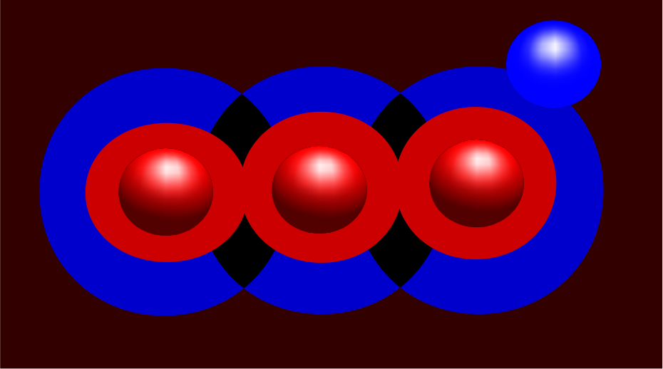
Consider an input system similar to the one described in Example Toy. with rigid molecular component augmented by a third atom with center . Then the minimum energy regions form two unconnected, parallel tori (black cross section shown in Figure 6). Since the regions are not connected, MC would need at least two random jumps/initial states to reach both regions. Our methodology treats both regions as lower dimensional boundaries that are guaranteed to be encountered in a parametrized exploration of any one of the three starting higher dimensional connected regions.
3.4 Cayley Parametrization for Efficiency
Locating boundary regions with minimal sampling during recursive search, as well as refinable sampling for volume computation are both challenging due to the disconnectedness and complexity of Cartesian active constraint regions (see Section 3.4.3). To address this challenge, we use a theoretical framework developed in the paper[6] (see Section B of the Appendix). Specifically, we map (many to one) a -dimensional Cartesian active constraint region , to a convex region of called the Cayley region of . Exploration of this convex region is direct and does not require enforcing the active constraints. In addition, the inverse map, taking an element of the Cayley region, a Cayley configuration to its finitely many corresponding Cartesian pre-image configurations is efficient to compute. For , each Cayley region corresponds to up to 8 contiguous Cartesian regions or macrostates called flips (defined in Section 3.4.2) and each Cayley configuration corresponds to up to 8 easily computable Cartesian configurations or microstates.
3.4.1 Convex Cayley Parametrization Theory
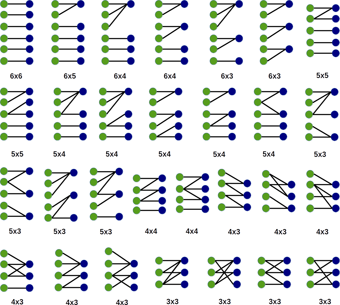
Define a non-edge of a graph as a vertex pair not connected by an edge in . One way to represent a higher dimensional active constraint region, i.e., with flexible configurations, is to use the realizable lengths of non-edges of its active constraint graph . By choosing non-edges whose addition make minimally rigid (see Section A of the Appendix), a tuple of realizable non-edge length values, a Cayley configuration, corresponds to finitely many Cartesian configurations. The non-edge length coordinates of a Cayley configuration are its Cayley parameters (see Section B of the Appendix). Finding Cayley parameters for an active constraint graph (for ) reduces to picking a (isomorphic) graph from Figure 7, with minimal number of vertices, (a minimally rigid graph, see Section A of the Appendix) for which is a subgraph. Thus, each active constraint region has its own region-specific set of Cayley parameters.
Consider the map from the Cartesian active constraint region of to the corresponding tuples of Cayley parameters (for those readers familiar with algebraic topology, we note that this map is a branched covering map [85, 86] that preserves dimension). The image of this map is the Cayley region of the active constraint graph . Sampling a Cayley region reduces to incrementing the Cayley parameters while staying within the region: the active constraints need not be explicitly enforced.
Definition 3.2 (Chart)
A chart for an active constraint region is the map taking a Cartesian configuration in to its corresponding Cayley configuration.
Certain classes of graphs, such as partial 3-trees (defined in Section A of the Appendix), yield convex Cayley regions with easily computable bounds [6] (see Theorem B.1 in Section B of the Appendix). Sampling in such active constraint regions with partial 3-tree graphs reduces to incrementing the Cayley parameters while ensuring that we stay within these easily computable bounds, and then computing the corresponding Cartesian configurations. Again, no explicit enforcing of active constraints is necessary. Section 3.6.1 describes how to sample regions and find Cartesian configurations in regions whose active constraint graphs are not partial-3-trees.
For small , almost all active constraint graphs arising from Assembly Problem (, ) are partial 3-trees and thus their regions have convex Cayley parametrizations. For , all the active constraint graphs with 1, 2 and 3 active constraints (5D, 4D and 3D atlas regions) are partial 3-trees. These are subgraphs of the graphs shown in Figure 7. of active constraint graphs with 4 active constraints (2D atlas regions) and of active constraint graphs with 5 active constraints (1D atlas regions) are partial 3-trees. Since, regions with 6 active constraints (0D atlas regions) have generically only finitely many (at most 8) Cartesian configurations in them, Cayley parametrization is irrelevant. See Section B of the Appendix for a more detailed discussion, including an example, on Cayley convexification.
Definition 3.3 (Atlas)
An atlas of an assembly landscape consists of the roadmap, and, for each active constraint region, (a) the Cayley parameters of the chart, and (b) a set of Cayley configurations and their corresponding Cartesian configurations.
Although most active constraint graphs arising in Assembly problem (, ) have convex Cayley regions, the feasible region is often (when in Constraint ) a non-convex subset created by cutting out regions defined by other constraints of type . Each such constraint resulting in a such a cut-out region is neither an active constraint nor a Cayley parameter in the active constraint graph. However, the cut-out regions typically have a (potentially different) convex Cayley parametrization. This can be seen in Figure 8 where the configurational region of the node in the center has a cut-out hole because of constraint violations by atom pairs that are not a part of the active constraint graph.
3.4.2 Computing Cartesian Configurations from a Cayley Configuration
The inverse map from Cayley configurations to Cartesian configurations can be computed easily since 3-trees (obtained by the addition of Cayley parameter non-edges to the active constraint graph) are realized by solving three quadratics at a time. This in conjunction with convexity of the Cayley region allows for efficient sampling of the typically disconnected and topologically complex Cartesian region (see Section 3.4.3).
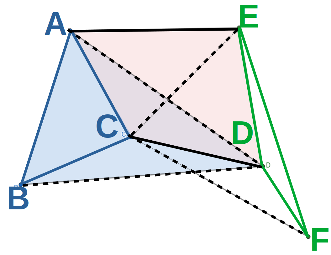
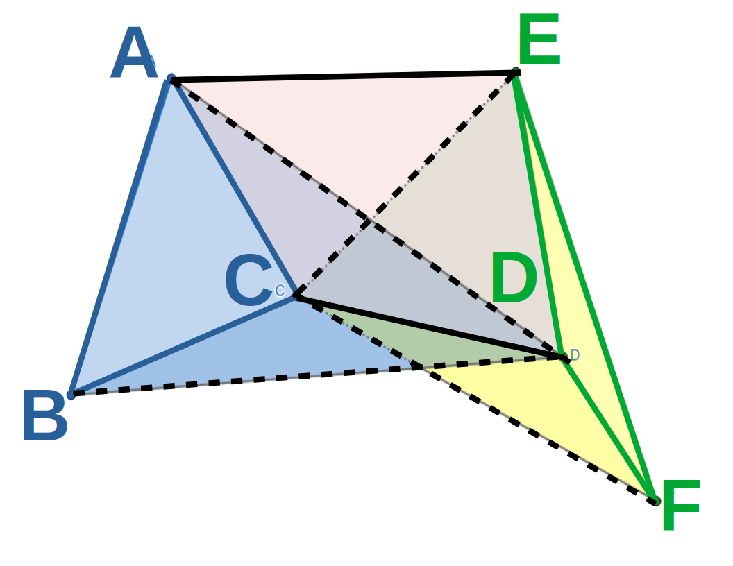
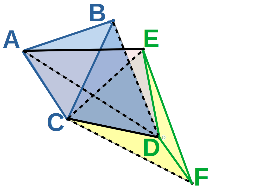
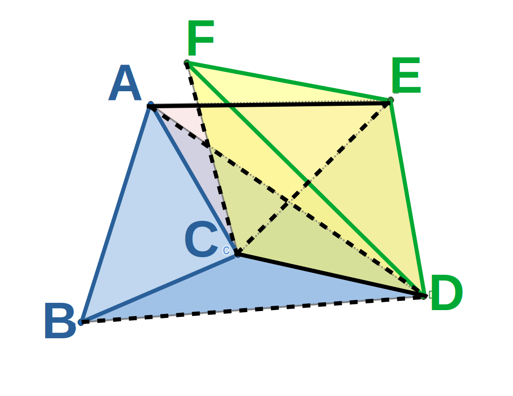
Realizing a complete 3-tree with tetrahedra means finding the coordinates of new points, one at a time, using 3 distance constraints between a new point and 3 already placed points. Each new point is the solution of the quadratic system for intersecting 3 spheres resulting in two possible placements of the new point. This yields possible Cartesian configurations of the Cayley configuration. A flip associated with an active constraint region consists of all Cartesian configurations in that region restricted to one of these placements (see Figure 9). For , there are always 3 tetrahedra and as a result, every Cayley configuration has up to 8 Cartesian configurations (see Theorem C.1 in Section C of the Appendix).
Flips could be disconnected and form distinct (Cartesian) macrostates. In addition, multiple flips could be connected to form a single macrostate when the tetrahedra flatten, which happens at the convex Cayley bounds (for those readers familiar with algebraic topology, we note that the Cayley parametrization map is a branched cover. See Section B in the Appendix).
3.4.3 Correspondence between Cayley and Cartesian Regions
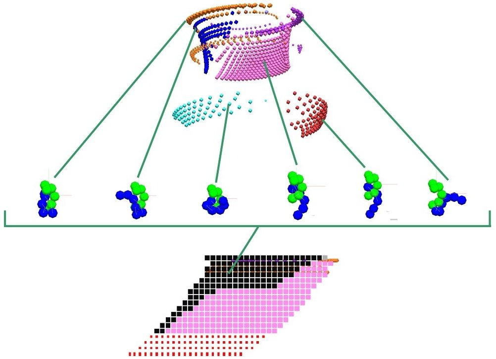
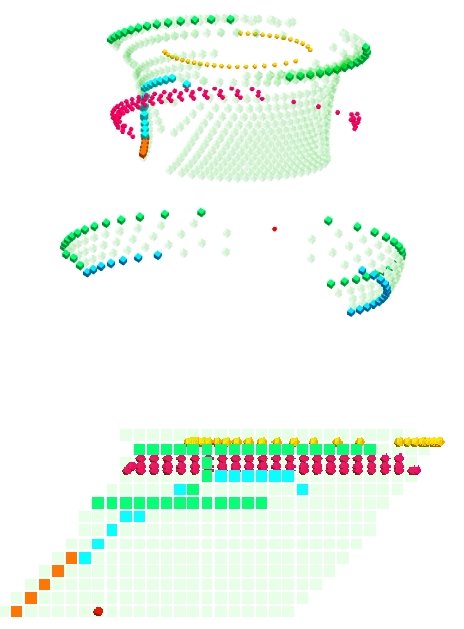
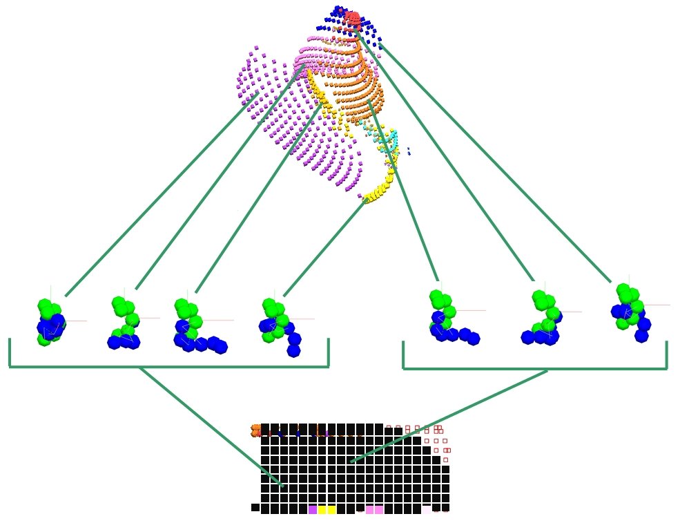
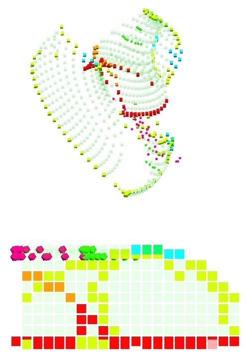
Figure 10 and Figure 10(b) show the stark difference in the topological complexity between the Cayley and Cartesian parametrization of two typical 2D active constraint regions. Each point in the bottom is a Cayley configuration. Each point in the top is a Cartesian configuration in the quaternion representation, i.e., as a point six dimensional space (3 translational and 3 rotational dimensions), projected onto the 3 translational axes.
Figure 10(a) and Figure 10(c) show the boundary or child regions of the active constraint regions of Figure 10 and Figure 10(b) respectively, where an extra constraint becomes active.
A Cayley configuration at the boundary of a parent region can map to multiple Cayley configurations in either the same or multiple children regions (via different flips and different region-specific Cayley parametrizations for the children). In the same way, multiple Cayley configurations at the same boundary in the parent region may map to the same Cayley configuration in a child region (via the same or different flips) due to different Cayley parametrization for parent and child.
3.5 Bar-Code: Input Shape Variables and Landscape Design Variables
We establish a formal and intuitive connection between the topology of assembly landscapes (output) and the geometry of the assembling rigid molecular components(input). The geometry of the input rigid molecular components is described by two input shape variables, the width of the rigid molecular component and its concavity. A rigid molecular component is considered narrow if the width of the entire rigid molecular component, defined as the spread of the rigid molecular component across its principal axis, is comparable to the average diameter of the ‘hard-sphere’ (described in Section 3.2) corresponding to constituent atoms. It is considered wide otherwise.
To measure the concavity of an input rigid molecular component, take a closed smooth manifold (skin), enclosing the minimum volume containing all the hard spheres corresponding to each of the constituent atoms in the rigid molecular component. For any two points on the skin of the rigid molecular component, consider the difference between their geodesic and Euclidean distance. Concavity is the average of all such differences across all pairs of points. Convex (resp. concave) rigid molecular components have low (resp. high) concavity. We can discretize concavity computation by reducing it to a discrete set of points for each atom that has at least a part of its surface on the skin.
The input shape variables can be tuned to ensure that specific active constraint regions and basins are present by influencing the landscape design variables (atlas bar-code). These are the number of active constraint regions and the average Cayley parameter range, where the average is taken over a set of active constraint regions of interest. The average Cayley parameter range for an active constraint region determines its volume. Furthermore, concavity of the input rigid molecular component, an input shape parameter, is directly correlated with the average Cayley parameter range and the volume of the active constraint regions.
Results in Section 4.2) show how the bar-code influences other dependent properties of the output landscape such as volume of regions and basins.
3.5.1 Advantages of Region-Specific Cayley Parametrization
There are 4 main advantages of region-specific Cayley parametrization.
1. Avoiding gradient descent: Since the Cayley region of an active constraint region is convex, and exact bounds are easily computed, sampling the region is as simple as taking a step within the convex Cayley bounds and computing the Cartesian configurations of the new Cayley configuration. This computation time is constant for any given as described in Section 3.4.2. This avoids gradient-descent search used by all prevailing methods to enforce the active constraints. With Cayley parametrization no constraints need to be enforced, drastically improving sampling efficiency and minimizing discarded samples.
2. Boundary detection: Sampling using region-specific parametrization reveals more configurations (see results in Section 4.3.3) and hence finds more lower dimensional boundary regions, decoupling the generation of the roadmap from sampling.
3. Volume computation: A child or boundary region may have negligible volume compared to the parent or interior region (as the child region has one lower effective dimension, for example a narrow channel in the assembly landscape). Yet, it deserves careful sampling when computing free energy and entropy since it has a lower potential energy level. Region-specific parametrization ensures better accuracy for sampling such regions as shown in Section 4.3.3.
Cayley convexification aids efficient approximate and exact volume computation. Approximate volume computation is used in the comparison of relative volumes of potential energy basins and computation of path probabilities (see algorithm in Section 3.7.3 and results in Section 4.4.1). Exact volume is used for entropy computation (see algorithm in Section 3.7.5 and results in Section 4.4.2).
4. Path Probabilities: To assign probabilities to paths between active constraint regions ( discussed in Sections 3.7.2 and 3.7.4) we can use two distinct partitions of an active constraint region into subregions, one based on the relative volumes of the parent regions and the second based on the relative volumes of children regions. These partition volumes along with paths between active constraint regions yields approximate path probabilities .
3.6 Algorithms
This section discusses the key algorithms implemented in the EASAL software [1, 3, 2]. We first present the core algorithm and analyze its correctness and time complexity. This is followed by 3 variants of the core algorithm for different assembly regimes: (1) arbitrary and ; (2) and ; and the most general version (3) with arbitrary and .
3.6.1 Core Algorithm
We describe the core algorithm for arbitrary and (Algorithm 1 in Section D of the Appendix), leveraging the capabilities described in the prior sections. The algorithm starts by generating all possible active constraint graphs with 1 or 2 (depending on user input) active constraints yielding 5D or 4D regions (represented as root nodes) in the roadmap.
Starting with an initially generated root node, the algorithm then (i) recursively (by depth first search) generates the roadmap by discovering active constraint regions of decreasing dimensions; (ii) uses Cayley convexification of the region to efficiently compute bounds for Cayley parameters a priori (before computing the Cartesian configurations), and coarsely samples Cayley configurations in this convex region; (iii) efficiently finds the (finitely many) Cartesian configurations of the sampled Cayley configurations; (iv) creates a boundary regions of 1 lower dimension when a new constraint becomes active detected as a collision a posteriori (after computing the Cartesian configurations). Configurations where a new constraint becomes active are witness configurations for the corresponding boundary or child region; (v) all ancestors of 0D regions are introduced into the roadmap, i.e., those missed by coarse sampling are later discovered by ancestor addition through their descendants, and sampled.
Thus, the algorithm, through coarse sampling, generates the roadmap, decoupling roadmap generation from sampling (as discussed in Section 3.2.4). Subsequently, a desired active constraint region can be sampled using different variants of Cayley sampling with any desired level of refinement. Optionally, as detailed in the pseudocode in Section D of the Appendix, the sampling can proceed along with the roadmap generation, resulting in a complete atlas.
Handling Non-Convexifiable Regions
When the active constraint graph of a region is not a partial 3-tree, we first drop constraints one at a time, until the active constraint graph becomes a partial 3-tree. In doing so, we end up in an ancestor region, with a partial 3-tree active constraint graph and a convex Cayley parametrization. Note that since non-partial 3-trees potentially arise only when exploring active constraint regions with 4 or 5 active constraints (2D and 1D atlas nodes respectively), it is always possible to drop one or two constraints to reach an ancestor region which has a partial 3-tree active constraint graph.
Once in the ancestor region, we trace along rays to populate the lower dimensional region by searching in the ancestor region. For example, to find a 2D boundary region which does not have a partial 3-tree active constraint graph or a convex parametrization, we drop one constraint resulting in a 3D parent region that is guaranteed to have a convex Cayley parametrization. We then perform multiple one dimensional searches in the 3D region (ray tracing) in order to locate the target 2D boundary (child) region along each of these rays, using binary search. This generalizes to any dimension and region in the sense that ray tracing is robust when searching for and populating a region one dimension lower. By recursing on the thus populated region, we find further lower dimensional regions.
3.6.2 Core Algorithm Accuracy
The discussion in the preceding sections proves the following theorem showing that the core algorithm finds the complete atlas of the assembly landscape (up to a tolerance specified as part of the input); overwhelmingly generates only feasible configurations, i.e., minimizes discarded samples; and only explores or samples any active constraint region once.
Theorem 3.4
(Completeness, Tightness and Efficiency) The core algorithm
- 1.
-
2.
only creates non-empty active constraint regions (through a witness configuration);
-
3.
only samples feasible configurations in active constraint regions with desired refinement;
-
4.
explores active constraint regions only once.
We emphasize a few notable features of the core algorithm. Lower-dimensional (boundary) regions are detected by detecting collisions. Binary search then determines, up to a tolerance, a witness configuration for creating this boundary region, ensuring that any created active constraint region is non-empty. Since children regions inherit the constraints of their parent regions, no region can be missed by not exploring the descendants of an empty region.
Once the boundary region is found, the core algorithm explores it using its region-specific Cayley parametrization. Therefore, even regions that have negligible volume in the parent’s parametrization, through their own parametrization, are as exhaustively sampled as the parent region.
In rare cases when there is no convex Cayley parametrization, the region is sampled as part of the parent region to ensure good sampling coverage.
In the core algorithm, we use a hash table to keep track of previously found and sampled active constraint regions. This ensures that active constraint regions, found through multiple parents, are not explored or sampled more than once.
Convexity guarantees that all sampled configurations (other than binary search due to collisions) are valid and none are discarded.
During binary search to locate a boundary region, after a collision, some samples may be discarded. Since this happens only once per newly discovered region from each ancestor region, the number of discarded samples is bounded by the number of edges in the roadmap DAG.
3.6.3 Complexity Analysis
Roadmap Generation
By Theorem 3.4 (1), (2), and (4)
the time to generate the roadmap is linear in the number of edges of the
roadmap DAG, since roadmap generation is decoupled from sampling.
In the worst case, the number of regions or nodes, , of the roadmap can be as large as .
Since the
complexity cannot be less than the output size, this achieves the best possible
complexity. Usually, is a much smaller number of regions specified as part
of the input by designating a set of active constraints of interest.
Sampling an Active Constraint Region
By Theorem 3.4 (1) and (3)
the sampling time grows linearly in the number of feasible configurations, which
in turn grows polynomially with sampling density and exponentially
in the dimension. The dimension of an active constraint region is bounded by
, where is the number of rigid molecular components. However, for any given the
dimension is a constant; hence the sampling time complexity is polynomial
in the sampling density.
Sampling time grows quadratically in the number of atoms in each rigid molecular component. This is because an a posteriori collision check involves, at worst, checking every atom pair (one from each rigid molecular component) for violation of the Constraint of the assembly problem. Note that this can be improved by using more sophisticated collision detection algorithms.
Thus, given a step size as a fraction of the range for each Cayley parameter, the complexity of sampling a region is , showing the expected tradeoff between complexity and accuracy [87]. The constant of proportionality hidden in the big depends on one of the two independent landscape design variables, i.e., the average Cayley parameter range as discussed in Section 3.5 (see Results in Section 4.5).
Sampling the Landscape
Putting these factors together, if is the number of regions to sample,
given as part of the input by specifying a set of active constraints of
interest, the complexity of sampling all these regions is . For a given number of rigid molecular components , the
complexity is linear in the number of regions , polynomial in the sampling
density and quadratic in the maximum number of atoms in a rigid molecular component . Note that number of regions is one of the landscape design variables.
The number of atoms is a constituent of the input shape variables.
A recent parallelized version of the EASAL software (using a modified version of the core algorithm) takes advantage of the partition of the landscape to sample active constraint regions in parallel without repeat sampling. The algorithm inherently does not present any obstacles to achieving a linear speedup with the number of compute cores. Early testing of this method has shown a 3X speedup on a 4 core machine.
3.6.4 Algorithm Variant for arbitrary and
Assembly Problem (, ) generalizes as follows. The constraint remains the same, the constraint now enforces a tree as the minimal active constraint graph, with one vertex (representing an atom) in each of the rigid molecular components. There are three distinct methods for tackling this variant of the problem.
In the first method we start by generating the assembly landscape of two rigid molecular components, say , . Then, treating each configuration in the atlas as a rigid molecular component we generate the atlas of . This way we add one rigid molecular component at a time till we have added all the rigid molecular components. With this method, at each stage, the number of atlases needed to be generated grows by a factor of the number of rigid configurations discovered at each stage. However, most of these configurations may not be valid further down the line. Thus this method does not scale well when the number of rigid configurations generated is large.
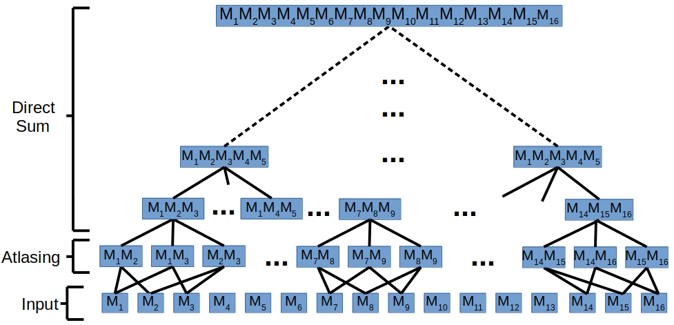
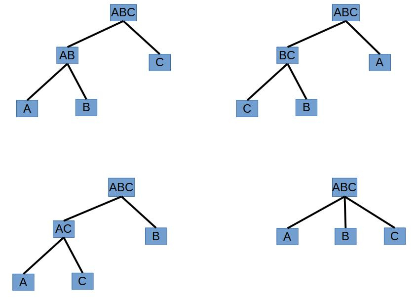
The second method is to generate, through atlasing, all the atlases of pairs of rigid molecular components, namely and for and . We then recursively merge by taking direct sums of these atlases, aligning the common rigid molecular components between them, and building larger atlases at every stage. This sets up a tournament tree, whose leaves are the input rigid molecular components, its internal nodes adjacent to the leaves are atlases obtained through atlasing, using the core algorithm, and all other internal nodes are obtained through a merging or direct sum of its children (see Figure 11). The root node is the final atlas of all the input rigid molecular components. At every internal node, the complexity of search is at most the product of the search complexity at all of its children.
For a given set of input rigid molecular components, there are potentially several different tournament trees. The optimal among these is the one which has the least search complexity at the root of the tree. Thus, picking of the best tournament tree can be setup as an optimization problem which minimizes the search complexity at the root of the tree.
Let us assume we are merging the atlases of , and to obtain the atlas . For a configuration in the direct sum, let configuration belong to the active constraint region of the atlas with graph and let configuration belong to the active constraint region of the atlas with graph . Now the configuration is a potential witness for the active constraint region with graph in the atlas for the 3 rigid molecular components. While we are guaranteed that all the configurations in the atlas for are contained in this direct sum, some configurations need to be removed. Specifically, we know that collision constraint holds between and either of the other two, but the configurations where does not not hold between and should be removed. These configurations can be eliminated using a simple collision check.
Second, configurations in an active constraint region with graph may additionally have a graph of active constraints between and . These configurations are witnesses for a new active constraint region with graph . However, this active constraint region need not be re-atlased, we can simply use the atlas of to look up the active constraint region with the constraint graph and merge it. This method is illustrated in Figure 12 for .
This method can be further optimized by indexing or hashing the active constraint regions (according to their active constraint graphs) and sample points (according to some Cartesian configuration metric). Indexing the active constraint regions allows us to look at a tiny portion of the assembly landscape instead of the whole thing at the same time giving constant time lookup when the active constraint graph is known. Indexing and hashing the sample points allows us to do range operations on them to either select or eliminate entire sets of configurations in an active constraint region, instead of having to look up individual ones every time we do a direct sum.
In this method, the number of atlases generated is always and all further atlases generated are done using simply by indexing and searching the previously generated atlases. If all ’s are identical, this method gains from the consequent symmetry in the landscape, since we just need to sample the configurational region of only one pair of molecular units and essentially reuse them.
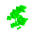
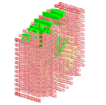
In the third method, we start by creating root nodes, whose active constraint graphs are the complete set of trees. There are trees with one vertex (representing an atom) in each rigid molecular component . If there are atoms in each , there are different active constraint graphs that are isomorphic to the same tree, and hence root nodes. Starting from the root nodes, we use the core algorithm, to recursively, by depth first search, generate the roadmap of the assembly landscape. In this method, we directly sample the dimensional space through Cayley convexification. Thus, for very large values of this method quickly becomes intractable. However, when all the ’s are identical, the number of root nodes is vastly reduced because the number of non-isomorphic (unlabeled) trees is much less than .
In fact, even when the rigid molecular components are not identical, we can exploit the existence of symmetries in the structure of the rigid molecular components to efficiently sample. The paper [9] studies all such symmetries in assembly landscapes. When each rigid molecular component is an identical singleton sphere, symmetries can be further exploited, leading to a much simpler algorithm, as explained in the next section.
3.6.5 Algorithm Variant for and
This variant of Assembly Problem (, ) is used in the study of particle cluster assembly (see discussion in 2.2). It is much simpler than the general input to our methodology since the presence of many isomorphic active constraint graphs lead to a large symmetry group for the assembly landscape. Utilizing these symmetries for this variant of the problem is discussed in the paper [9] and summarized in Section E of the Appendix.
In particular, the symmetry (isomorphic active constraint graphs) allows the potential stratified roadmap to be created apriori, with only one copy of each unlabeled active constraint graph, i.e., the fundamental domain of the full roadmap. The core algorithm proceeds as usual but its function is to remove all descendants of a region that has no witness configurations (see Algorithm 2 in Section F of the Appendix.)
As Theorem E.1 in Section sec:app:symmetries of the Appendix shows, in
addition to the symmetry in the roadmap, there are symmetries within active
constraint regions themselves. For many active constraint regions it is
sufficient to sample a portion whose symmetry orbits complete the region.
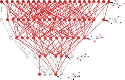
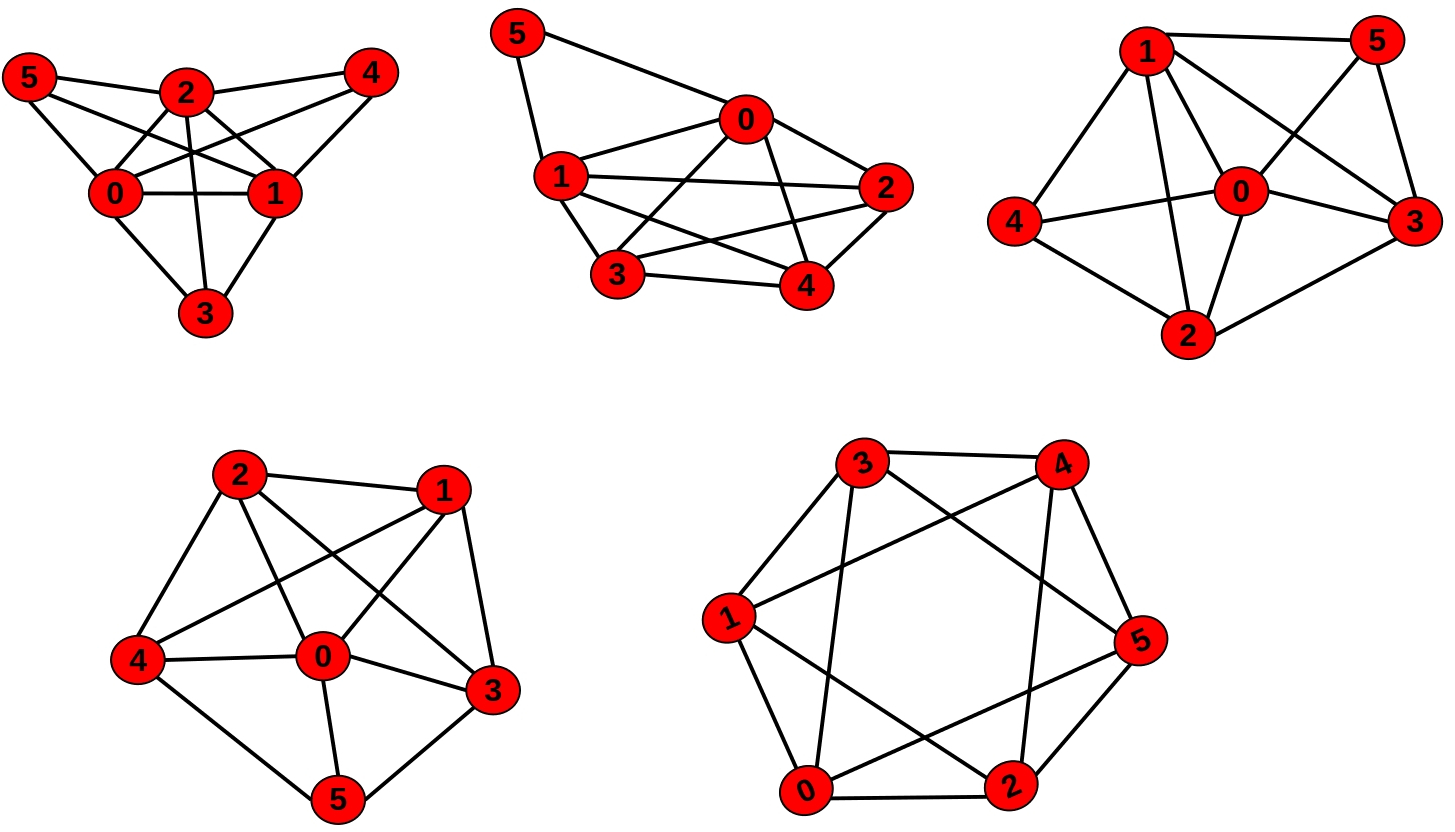
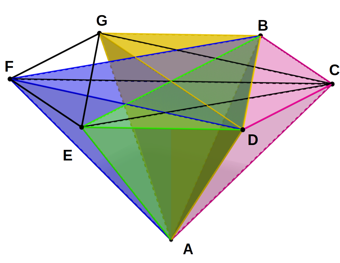
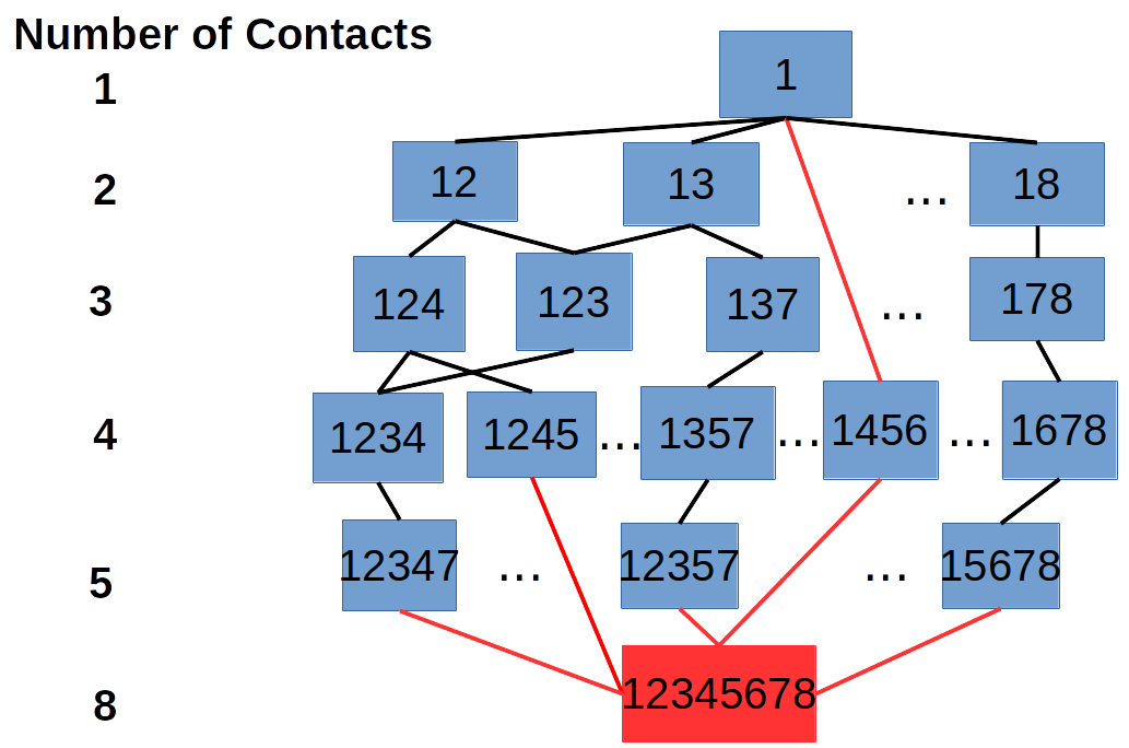
Illustrative Example: Consider an assembly system of identical hard spheres with pairwise distances equal to the sum of the hard-sphere radii. Since all particles and all interaction distances are identical, two isomorphic active constraint graphs represent the same active constraint region and only one representative is needed in the atlas. Figure 13 shows the fundamental domain of the atlas (up to 4D regions). The red nodes have non-empty active constraint regions while white nodes have no feasible configurations. On the right, we show the active constraint graphs of some active constraint regions. The roadmap has exactly five 0D regions, which correspond to the 5 non-isomorphic rigid active constraint graphs shown in Figure 14.
3.6.6 Algorithm Variant for arbitrary and
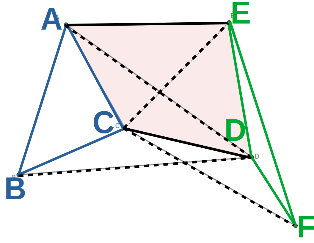
For arbitrarily large and , some decomposition based method is required to tractably deal with the size of the assembly landscape. The concept of decomposition and recombination plans or DR-plans is useful in this context [88, 89, 78]. Generally there are several ways to combine the solutions to sub-assemblies. The overall complexity of the recombination process depends primarily on the maximum number of sub-assemblies combined at a stage. Figure 15 shows all the different ways of combining sub-assemblies into larger assemblies, when we are given rigid molecular components , , and as input. In general, we choose a DR-plan where the number of sub-assemblies being combined at any given stage is at most 12. Now, the third method from Section 3.6.4 can be used at each stage. In particular, if the number of sub-assemblies being combined at any given stage is at most 2, as in the first three cases of Figure 15, then one of the first two methods of Section 3.6.4 can be used.
3.7 Algorithm Extensions
This section describes algorithms to compute several direct byproducts of the atlas: (1) structure and neighborhood relationships of potential energy basins, (2) paths between active constraint regions and basins, (3) approximate basin volumes, (4) path probabilities and (5) entropy integrals.
3.7.1 Algorithm for Potential Energy Basin Structure
The lowest potential energy region of a basin or basin bottom is typically, but not always, an effectively 0-dimensional active constraint region , with graph , that splits into finitely many basins whose bottoms are rigid configurations satisfying the constraints in . The potential energy basin (basins) corresponding to include portions of all ancestor active constraint regions whose graphs are non-trivial subgraphs of . Hypostatic basins have higher dimensional active constraint regions as ‘bottoms’, i.e., their active constraint graphs are maximal with no additional constraints possible, but their configurations are flexible. In this manner the assembly landscape is partitioned into potential energy basins with clear neighborhood relationships. Free energy of a configuration depends both on the potential energy and the weighted relative volume (entropy) of its potential energy basin.
Figure 16 schematically uses a 6-simplex to illustrate the structure of a potential energy basin (up to 3D regions). Specifically, it illustrates how multiple active constraint regions (3D-0D) interact to form the basin. In the figure, vertices B through F represent constraints between atoms and A is a dummy vertex used for visualization. Each of the 20 tetrahedra represents a 3D active constraint region, with Tetrahedron ABCD representing the region in which the constraints E, F, and G are active. Each of the four colored tetrahedra share a common triangle ABD, whose active constraints are C, E, F, and G, i.e., the triangle 2D region ABD is a boundary of each of the colored tetrahedral 3D regions formed by adding one more constraint to each of their active constraint graphs.
Figure 16 shows how active constraint regions interact in a generic setting. Figure 16 shows a non-generic setting. In addition to non-generic hypostatic basins previously discussed, there is a further type of non-genericity where more than one constraint becomes active at the same time.
Figure 16 schematically illustrates a hyperstatic regions and potential energy basins. Each box represents an active constraint region and the numbers inside the boxes represent the set of active constraints. The figure shows a portion of the roadmap for nodes that have the active constraint ‘1’ in them. Generically, when going from a parent to child regions, only one more constraint gets added to the set of active constraints. However, in some non-generic cases (shown as red edges), multiple constraints get added simultaneously. For example, the edge between 1 and 1456, causes a drastic reduction in energy/effective dimension from parent to child when compared to a generic case. It also creates a higher potential energy barrier when going from a region to its parent as multiple bonds need to be broken simultaneously. Recalling , the ambient dimension of the assembly problem, generically, basins correspond to active constraint regions with ) constraints with rigid configurations, but in hyperstatic basins more than constraints could become active (e.g., red node at the bottom with 8 constraints).
Crucially, since the core algorithm recursively generates the roadmap from interior to boundary (higher to immediately lower energy/dimension), the hypostatic basins are guaranteed to be found. Hyperstaticity - when multiple constraints become active simultaneously - is easily handled by the core algorithm by creating clearly marked dummy nodes that fill out the intermediate energy/dimension levels of the stratification, ensuring that only one extra constraint is added in any parent child relationship. These dummy nodes are not included in the count of active constraint regions (a landscape design variable). Results for potential energy basin structure are presented in Section 4.3.1.
3.7.2 Finding Paths between Active Constraint Regions
From the generated roadmap, it is extremely fast to find (shortest) paths (or number of paths of a given length) below a given energy level, between any two active constraint regions. Of particular interest is finding paths between two 0D active constraint regions that generically correspond to basin bottoms. Specifically, we are interested in paths through 1D regions (with one higher degree of freedom and one fewer constraint). These regions represent a generic one degree of freedom motion path (see Figure 17).
Moving from one 0D region to another via a 1D region involves releasing a constraint and making the same or a different constraint active. This corresponds to crossing a local energy barrier. Breaking more than one bond at a time means crossing a larger energy barrier. Either one (shortest) path or all of them between two given active constraint regions are found by performing a standard breadth first search through the roadmap DAG. Alternatively, the number of paths of a given length can be found by performing a matrix multiplication on the adjacency matrix of the DAG restricted to the relevant energy/dimensional regions (see results in 4.2.4).
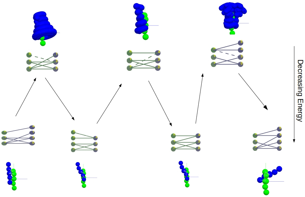
3.7.3 Approximate Basin Volume Computation
To compute the volume of a potential energy basin for a given ‘bottom’ active constraint region with constraint graph , we first identify all active constraint regions with . Not all configurations in contribute to this basin since is part of all basins with bottom regions with . Hence we locate those configurations in that are ‘close’ to some boundary region with . For all , the total number of these configurations, is the approximate volume of the potential energy basin.
To find the configurations in that are close to a boundary region , we use a method of partitioning the set of configurations of any parent region into sub-regions one for each child boundary region. For example, a given 5D region can be partitioned into sub-regions, one for each of its 4D children. The sizes of the sub-regions are proportional to the relative sizes of the boundaries corresponding to children, since the size of the boundary is a proxy for the probability that the new constraint corresponding to that boundary becomes active.
Let be the size of the boundary region in the parent , based on the number of sampled configurations in . Then, the relative size of the boundary is given by and the number of configurations that lead to a boundary region is then the product of and the number of configurations in .
While different Cayley parameters choices for could lead to different sizes of boundaries, the relative sizes of the boundaries are independent of the choice of Cayley parameters. Nevertheless, using Cayley configurations, as opposed to Cartesian configurations, to compute these quantities only provides an approximate basin volumes (see results in Section 4.4).
3.7.4 Computation of Path Probabilities
The probability of a path between two active constraint regions is the product of the probabilities of each directed edge in the path. The directed edges are either edges in the roadmap DAG or their reverse. For a directed edge from a region to in the roadmap DAG, the probability is the relative size of the boundary corresponding to within . This is computed as described in Section 3.7.3.
The following example shows how to compute the probability on the reverse edges. Consider a simplified atlas which has two active constraint regions and that are root nodes in the roadmap DAG, i.e., they have no ancestors. Let (resp. ) be the probabilities of a configuration being in (resp. ); can be computed as the relative volumes of and using the same Cayley parameters. If and are not root node regions, can be computed by treating and as bottoms of basins and computing their relative volumes as described in the previous section, but using common Cayley parameters.
Let and be children of both and . Let be the probability of the roadmap DAG edge and let be the probability of the roadmap DAG edge , computed as described above. Since and are the only children of and , the probabilities on the edges and . Thus, the probabilities of a configuration being in and are given as follows.
Let be the unknown the probability of a configuration in having come from on the addition of an active constraint, which is treated as the probability of ending up in after a constraint is released. Therefore the probabilities , and . Similarly, take and . Now we can solve for unknowns and using the following two equations.
Once and are solved for, the probability of the path , for example, can be computed as and the probability of path can be computed as .
Using the computation of the partitioning probabilities described above (, and , , in the above example), and the algorithm for finding paths between active constraint regions (described in Section 3.7.2), probabilities for atlas paths can be computed.
3.7.5 Computing Cartesian Integrals using the Cayley Region
Metric on modulus space A single flip of a Cartesian active constraint region of dimension is a -dimensional manifold in . Six of the dimensions represent rigid body motions that should not enter the metric. Fortunately, every Cartesian configuration output by our methodology represents a unique orbit of the manifold modulo the special Euclidean group of rigid body motions (for those readers familiar with algebraic topology, we note that the branched covering map gives a bijection between each Cartesian flip and its corresponding Cayley image).
The distance of two orbits with orbit representatives can then be defined as the minimal Euclidean distance between Cartesian configurations from the orbits:
For two Cartesian configurations , the projection of on the local tangent space of is
Entropy Integral The partition function for a manifold can be expressed as the integral[47].
| (2) |
where is called vibration factor, rotation factor and is the metric on . To compute the integral using the Cayley parameter samples output by our methodology, we convert Eq. (2) into an integral on the Cayley parameters :
| (3) |
where where is the Jacobian matrix when changing variables from Cartesian coordinates to Cayley parameters . To approximately calculate for each , we find a Cartesian configuration with Cayley parameters , we find the Cartesian configurations of the Cayley parameters and project the into the tangent space of as . Then
To capture multiple flips and to account for different isomorphs of the same active constraint graph(for example when the rigid molecular components are identical), the integral over the Cartesian active constraint region in the fundamental domain of the roadmap is determined as . The Jacobian matrix has been used to develop a sophisticated adaptive sampling method, different from the one presented in this paper, that samples the Cayley region to get a guaranteed uniform coverage of samples in the Cartesian region. This adaptive Jacobian algorithm, is the subject of a companion paper [75].
4 Results
Results demonstrating the core algorithm’s capabilities and high computational efficiency have been generated by a resource-light, curated opensource software implementation EASAL [1] (Efficient Atlasing and Search of Assembly Landscapes, see software [2], video [3] and user guide [4]).
We present 4 types of results demonstrating features of the new methodology that were described respectively in Sections 3.2, 3.3, 3.4, 3.6.3, 3.7.1, 3.7.2, 3.7.3, and 3.7.5.
(1) Landscape Design and Path Finding. Section 4.2.2 demonstrates the connection between input shape variables and the two landscape design variables described in Section 3.5, namely the number of active constraint regions and the average Cayley parameter range.
Section 4.2.2 shows how the volumes of active constraint regions can be designed by varying the concavity of the rigid molecular components.
The independence of the two landscape design variables and their precise effect on the total assembly landscape volume is demonstrated in Section 4.2.
Section 4.2.3 demonstrates the effect of the two landscape design variables on the volumes of the different dimensional (energy) strata, both of the atlas and individual basins. Together the landscape design variables provide a bar-code summarizing the atlas. In addition the effect of the input shape variables on the bar-code is shown.
Section 4.2.4 shows the efficiency of computing paths between active constraint regions once the roadmap has been found.
(2) Recursive Search and Decoupling of roadmap generation from sampling density. Section 4.3 first shows the diminishing returns of number of samples in finding the regions of the roadmap.
Section 4.3.1 shows the use of recursive boundary search for finding diverse types of basins and their bar-codes.
Section 4.3.2 quantifies how recursive boundary search decouples both efficiency and accuracy of roadmap generation from sampling density.
Section 4.3.3 quantifies how region-specific parametrization aids in decoupling.
(3) Volume Computation for Potential Energy Basins. Section 4.4.1 demonstrates the efficiency of computing approximate basin free energy i.e., volumes stratified by their dimension or energy.
Section 4.4.2 gives results on accurate volume and entropy computations for the case of and , i.e., cluster assembly from identical spheres.
(4) Verifying the Theoretical Time Complexity from Section 3.6.3. Section 4.5 tabulates computational experiments verifying the time complexity analysis for the single threaded version of EASAL, in particular showing the dependence of the sampling time on the landscape design variables and the input shape variables.
4.1 Details of the Experiments
We describe the experimental setup in Section 4.1.1, the main computations in Section 4.1.2 and the key measurements in Section 4.1.3.
4.1.1 Experimental Setup
The experiments were broadly run on two types of input.
(1) The results for input rigid molecular components (macromolecular assembly, Sections 4.2.2, 4.2.4, 4.3.1, 4.3.2, 4.3.3, 4.4.1, and 4.5) are set up to cover a wide variety of geometric shapes (input shape variables, including number of atoms, concavity and width, see Figure 18). Although the proof of concept results here, are restricted to atoms, EASAL has been used to analyze assemblies of rigid molecular components with atoms [10].
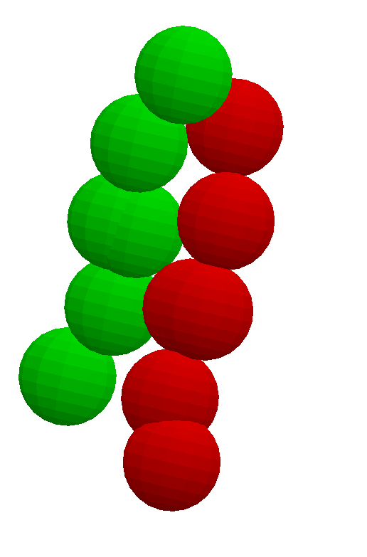
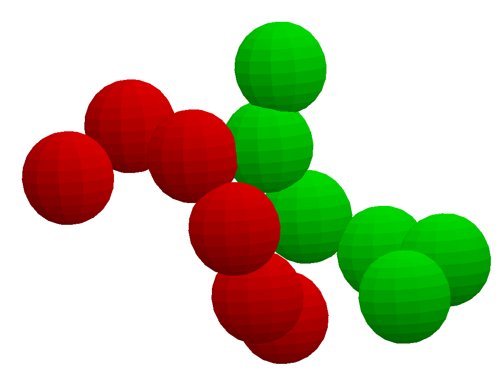
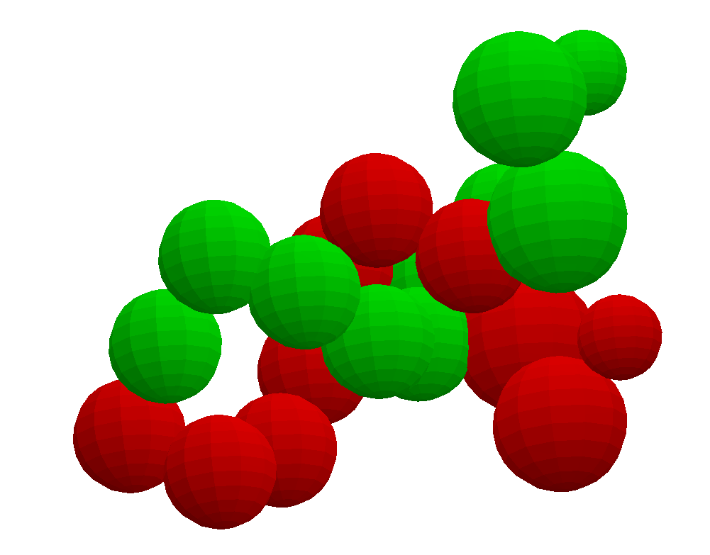

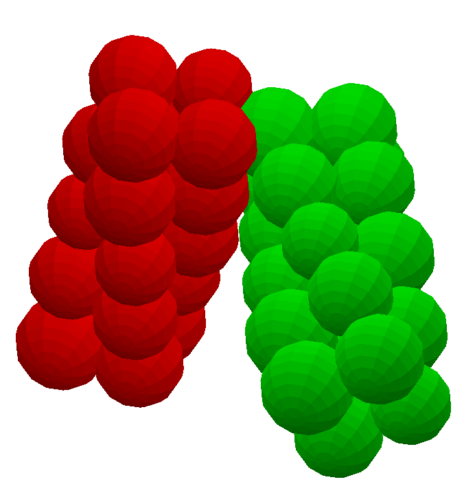
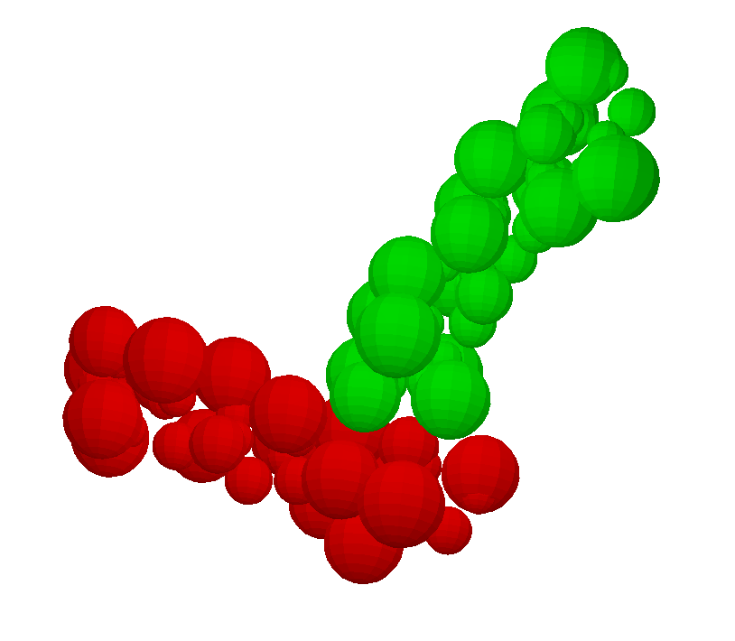
The width of input rigid molecular components Figure 18 - Figure 18 is comparable to the average diameter of their constituent atoms and hence considered narrow. The width of the rest of the input rigid molecular components (Figure 18 - Figure 18) are much greater than the average atomic diameter and are hence considered wide.
The experiments were run on a laptop with Intel(R) Core(TM) i7-7700 @ 3.60GHz CPU with 16GB of RAM. Suitable g++ compiler optimizations were used on the EASAL code (open source software available on Bitbucket at https://bitbucket.org/geoplexity/easal) to enhance its performance. On average 52 million configurations were generated per hour.
(2) The results (spherical cluster assembly, Section 4.4.2) are setup as follows. Each assembly system consisted of identical singleton spheres. The experiments were run on a laptop with Intel(R) Core(TM) i5-2500K @ 3.2GHz CPU with 8GB RAM. For , on average, 4 million Cartesian configurations in the underlying fundamental region of the roadmap (up to 3D active constraint regions) were generated per hour.
4.1.2 Main Computations
We perform 3 main computations.
(1) Atlas Generation. For (shown in Figure 18), we generate the atlas for 10 typical randomly chosen 5D active constraint regions and all their descendants. To be able to compare the results across rigid molecular components, we fix the ratio of the average atom radius to the sampling step size . We additionally fix the width of the Lennard-Jones’ well, in Assembly Problem (, ) for an atom pair , with radii and , to . Each of these input assembly systems was sampled with 3 different values of , to analyze the effects of step size on the sampling time. The core algorithm in Section 3.6.1 is used to generate the atlas.
For , the fundamental domain of the atlas was generated for 0D to 3D active constraint regions. The algorithm variant in Section 3.6.5 is used.
(2) Basin Mapping and Volume Computation. The input is a previously generated atlas and an active constraint region whose corresponding basin is to be mapped. All ancestor regions that contribute to the basin are generated (by taking subgraphs of the active constraint graph of the input region). To compute the volume of the basin, the algorithm described in Section 3.7.3 is used.
(3) Path Finding. The input is a previously generated atlas and 100 randomly chosen pairs of active constraint regions. To find the shortest paths and the number of paths of a given length, the algorithm in Section 3.7.2 is used.
(4) Entropy integral. The input is a previously generated atlas (). The algorithm described in Section 3.7.5 is used.
4.1.3 Key Measurements
(1) The number of active constraint regions, a landscape design variable, is measured both for atlases and basins.
(2) The average Cayley parameter range, a second landscape design variable (defined in Section 3.5), is measured for atlases regions.
(3) The weighted samples are the number of Cayley configurations sampled, weighted by the number of their corresponding Cartesian configurations. This is measured both for atlases and basins.
(4) We measure the time required for atlas, basin and path computation.
4.2 Results on Designing Landscapes and Finding Paths
To validate the discussion in Section 3.2, we show how to design assembly landscapes, by using the input shape variables, to alter the landscape design variables. We analyze the independence of the two landscape design variables and their precise effect on assembly landscape volume. We show how volumes of active constraint regions are designed by changing the average Cayley parameter range for the region, a landscape design variable. Time required to compute both the shortest path and the number of paths of a given length are tabulated.
4.2.1 Independence of the two Landscape Design Variables
The goal of this experiment is to verify that (a) the independence of the two landscape design variables, namely the number of active constraint regions and the average Cayley parameter range; and (b) that the number of weighted samples, a proxy for volume, is linear in the number of regions where the linear factor depends only on the average Cayley parameter range and the sampling step size. This validates the discussion in Section 3.5.
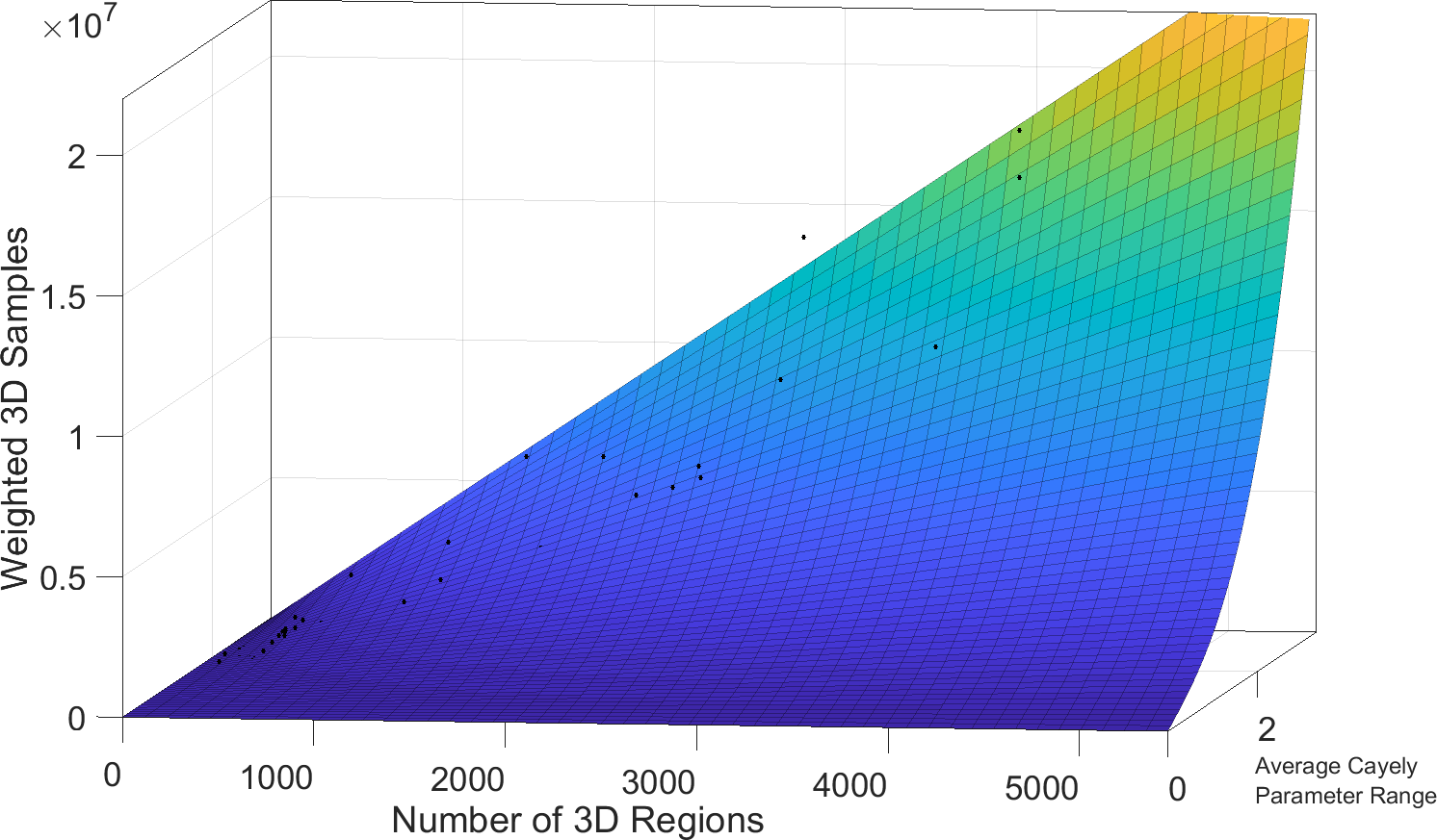
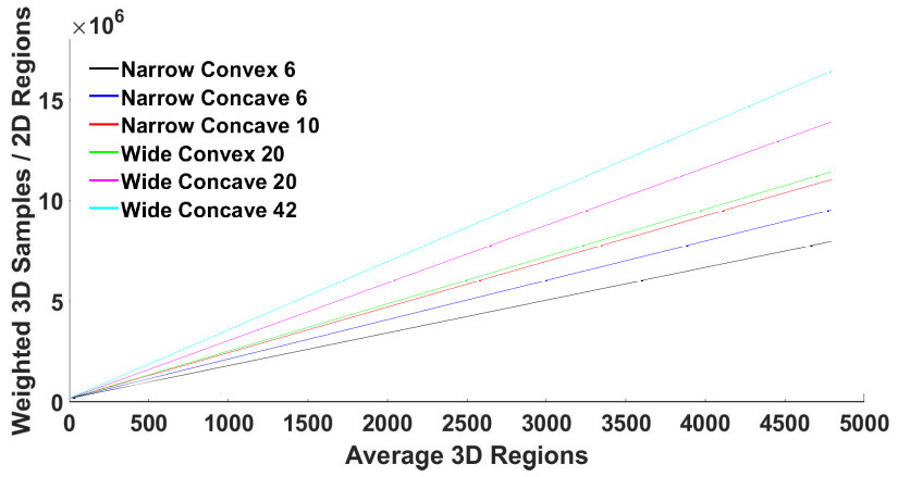
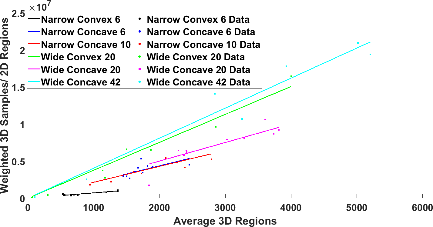
Figure 19 plots the average Cayley parameter value and the number of 3D regions against the number of weighted samples in those 3D regions. These regions are the descendants of the 10 5D regions for the 6 input rigid molecular component pairs described in Section 4.1.1. Each point represents a single atlas for one of the input rigid molecular component pairs.
We expect the number of weighted samples to vary as the third power of the average Cayley parameter range and linearly in the number of regions. As predicted, a bivariate function that is cubic in the average Cayley parameter range and linear in the number of active constraint regions shows a good fit to the points.
Figure 19 shows 6 slices of the plot in Figure 19 taken at values corresponding to average 3D regions’ Cayley parameter ranges, for each of the 6 input rigid molecular component pairs.
Independently, for each input rigid molecular component pair, Figure 19 plots the number of 3D regions against the number of weighted samples in those regions. As can be seen, the predicted plots (Figure 19) and the observed plots (Figure 19) match except for the 20 atom wide concave and the 20 atom wide convex systems, which have switched order. We expect this is because of the highly non-generic nature of the wide convex rigid molecular component which has several atoms with similar radii.
4.2.2 Designing Volumes of Regions via Average Cayley Parameter Range
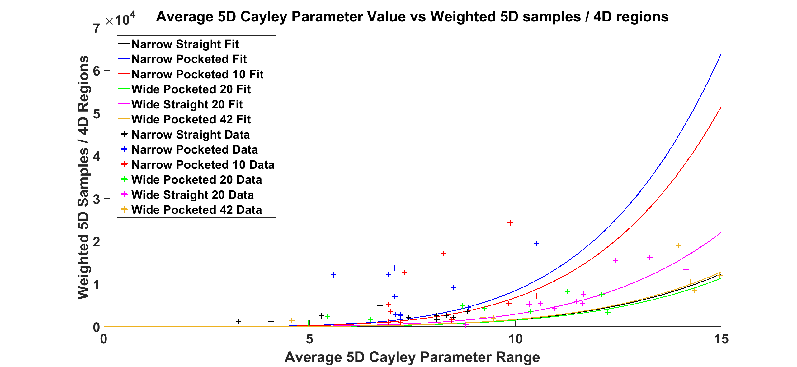
The goal of the experiment is to verify that the volumes of active constraint regions can be designed using the average Cayley parameter range, a landscape design variable, which in turn can be tuned using the input shape variables.
However, once the Cayley parameter range is fixed, we expect the number of weighted samples to be the same across all rigid molecular components regardless of their size and their geometry.
We present results validating the discussion in Section 3.5, by demonstrating that the number of weighted Cayley samples (a proxy for volume) in an active constraint region is proportional to its average Cayley parameter range raised to its dimension.
To be able to compare the effect of the average Cayley parameter range on weighted samples across different rigid molecular components, we divide the average Cayley parameter range by the average radius of the atoms in the input rigid molecular components. In addition, we correct for the extra samples created by boundary search. While finding the boundaries of an active constraint region, the EASAL software performs binary search (described in Section 3.6), which leads to the creation of more samples. The number of extra samples created in an active constraint region due to binary search is proportional to the number of children of that region. Hence we divide the number of weighted samples in the active constraint region by its children.
Therefore in Figure 20, the x-coordinate represents the normalized average Cayley parameter range value for that active constraint region obtained by dividing it by the average radius of atoms in the input rigid molecular components. The y-coordinate represents the number of weighted samples in the active constraint region divided by the number of its children.
Figure 20 shows trend lines of the variation of weighted samples with the normalized average Cayley parameter range. It is clear that the trend lines match the a degree polynomial fit from MATLAB, where is the dimension of the active constraint region. The results are shown for .
4.2.3 Using the Bar-Code of the Atlas
This experiment demonstrates a surprising behavior of the succinct bar-code (shown in Figure 21) of Section 3.5. The bar-code consists of (1) the normalized profiles of the two landscape design variables and (2) the weighted samples of the output atlas or basin, both stratified by dimension. The experiment shows that the bar-code does not change appreciably with variations in the input shape variables of the 6 input rigid molecular component pairs. This is despite the strong influence of input shape variables on the absolute values of the landscape design variables of the atlas as a whole, of individual regions, and of dimensional strata, as demonstrated in the previous two experiments.
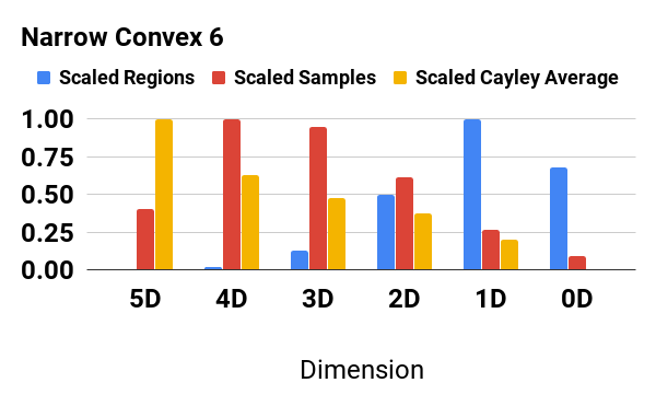
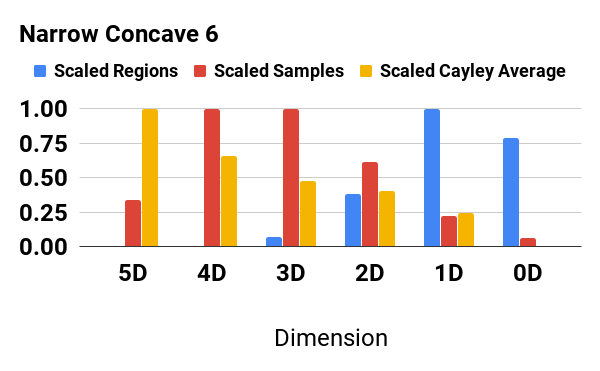
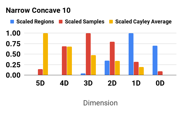
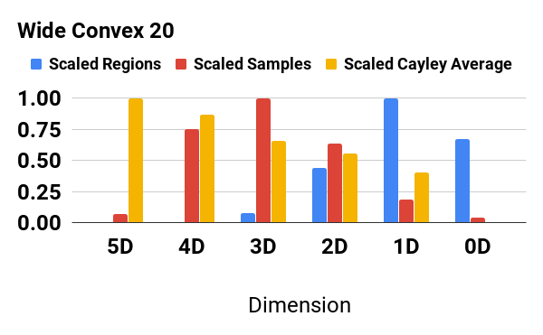

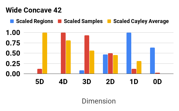
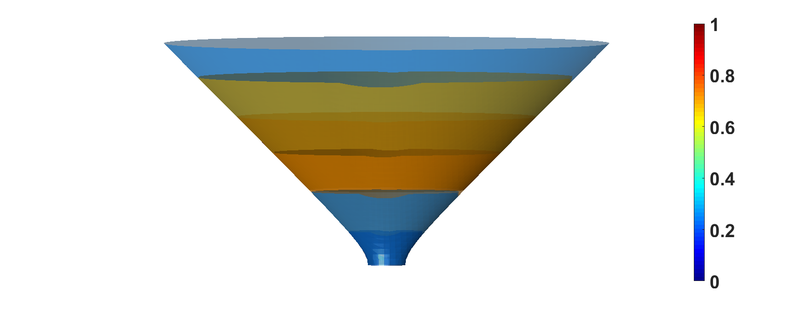
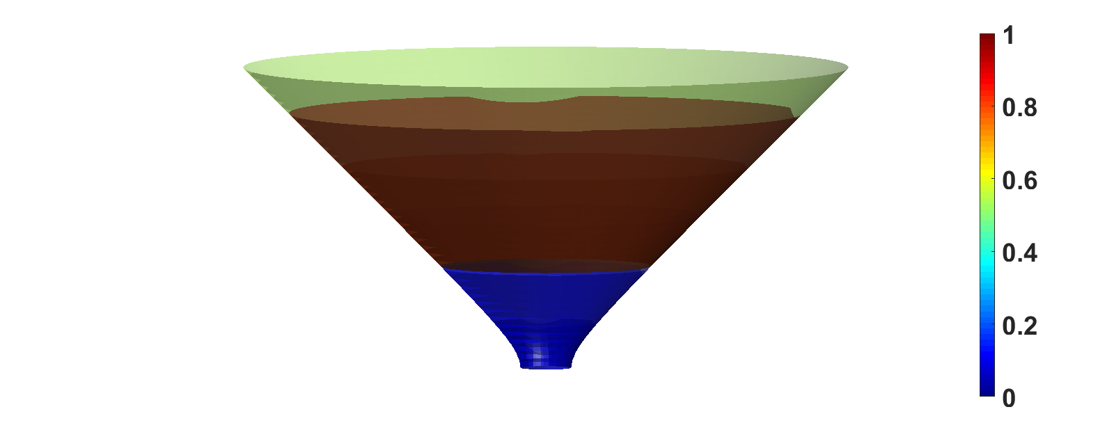
In other ways, however, the bar-code behaves as expected. The highest number of regions belong in the lower dimensional strata (0D, 1D, 2D) and a negligible number belong in the higher dimensional strata (5D, 4D, and 3D). Despite this, as expected, the total number of samples in higher dimensional regions is significantly higher than those in lower dimensional regions, due to exponential dependence on dimension. In addition, the higher dimensional regions also have higher values of the average Cayley parameter range, which decreases exponentially by dimension. The bar-code for the basin behaves similarly to the bar-code of the atlas.
4.2.4 Finding Paths from Roadmap
The goal of this experiment is to tabulate the time that the algorithm of Section 3.7.2 takes to find shortest paths and number of paths between active constraint regions of previously generated atlas. The experiment was run on the atlases of the narrow convex 6 and the narrow convex 20 rigid molecular components. The results are summarized in Tables 2 and 3.
| Path Length | Time | ||
|---|---|---|---|
| 6 | 176 | 7 | 1.9 ms |
| 6 | 145 | 6 | 2.2 ms |
| 20 | 787 | 18 | 119ms |
| Time | |||
|---|---|---|---|
| 6 | 176 | 2 | 2.02 s |
| 176 | 4 | 4 s | |
| 176 | 8 | 6.04 s | |
| 176 | 10 | 8.08 s | |
| 20 | 787 | 2 | 6 min |
| 787 | 4 | 11.58 min | |
| 787 | 8 | 18.04 min | |
| 787 | 10 | 27.44 min |
4.3 Results on Recursive Search and Decoupling
We demonstrate the core algorithm’s effective decoupling of roadmap generation from sampling discussed in Section 3.3.1.
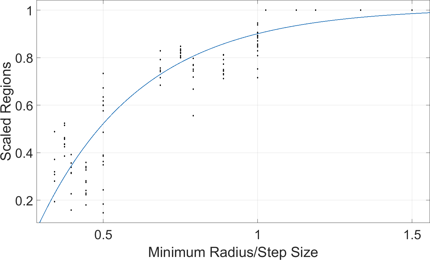
|
\bottominset
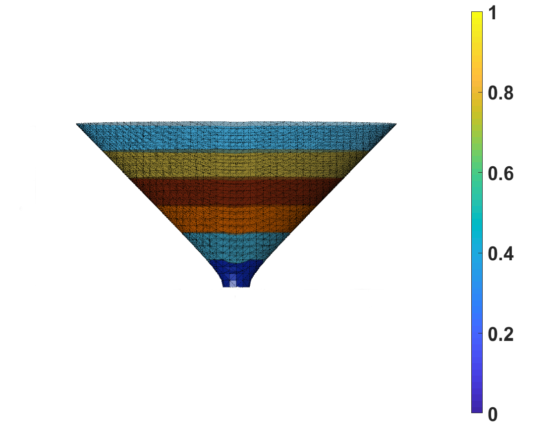
30pt18pt
\bottominset
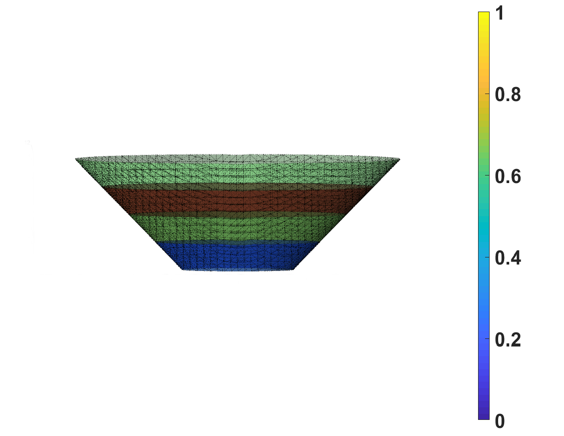
20pt30pt
\bottominset
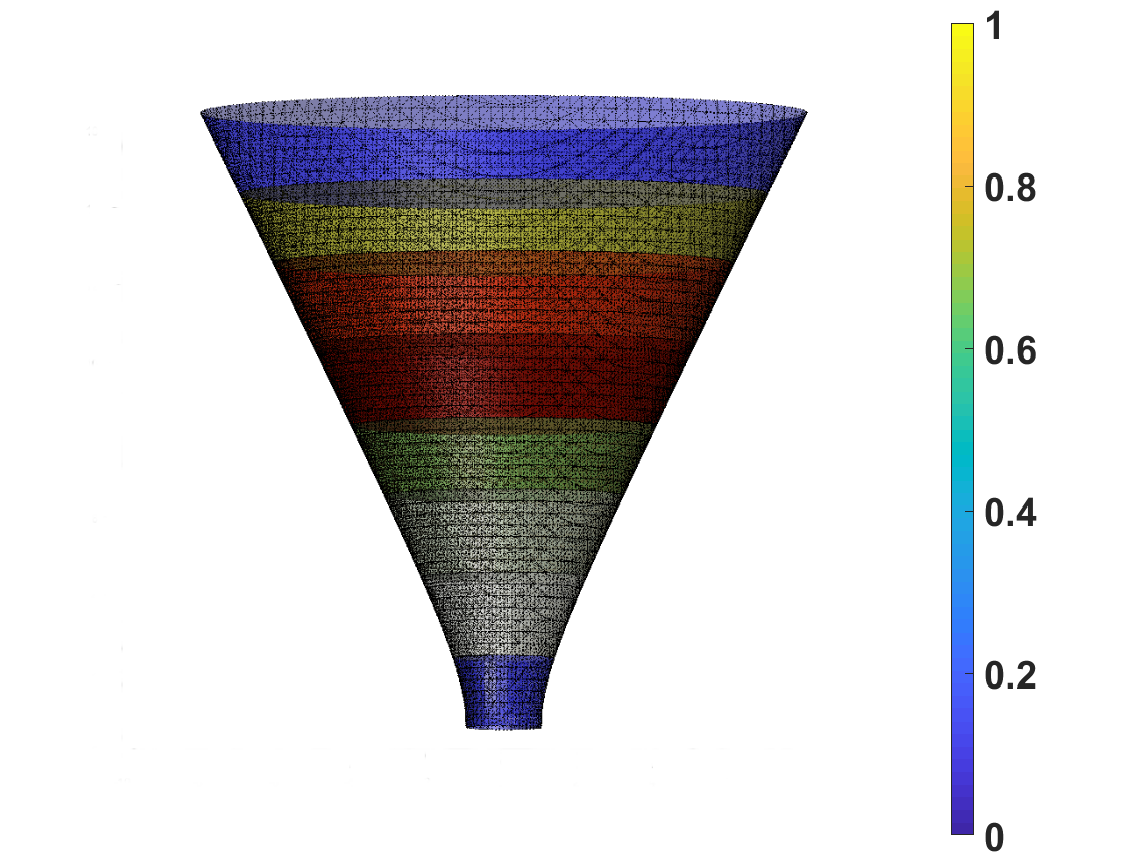
10pt20pt
|
The first experiment shows that decreasing the step size (a way to get better coverage of the configurational region), gives diminishing returns in terms of the number of regions discovered. To be able to compare the phenomenon across the 6 different input rigid molecular component pairs, we normalized the step size by dividing it by the radius of the smallest atom in the input rigid molecular component pair.
In Figure 22, we plot the ratio of the radius of the smallest atom in the assembly system to the step size on the x-axis and on the normalized number of regions discovered using this step size on the y-axis. Each point represents one run starting from one of the 10 5D regions, for one of the 6 input rigid molecular component pairs, for one of the step sizes, as described in Section 4.1.1. As the step size decreases the number of regions discovered converges. Specifically, as the step size approaches the radius of the smallest atom in the assembly system, the number of regions discovered does not significantly increase. This supports the effectiveness of our methodology in generating the roadmap with minimal sampling and thus decoupling roadmap generation from sampling.
4.3.1 Recursive Search for Locating and Mapping Basins
This experiment demonstrates that the recursive approach to roadmap generation easily locates all three types of basins (normal, hypostatic, and hyperstatic) and maps their structure using the algorithm in Section 3.7.1.
Figure 23 schematically shows a portion of the basin bar-code, i.e., the number of ancestor regions of different dimensions that contribute to different types of basins occurring in the assembly landscapes of of 3 different input rigid molecular component pairs.
Figure 23(a) shows the basin bar-code for the 6 atom narrow concave system, a generic basin.
Unlike the generic basins shown in Figure 23(a), the basin bar-code in Figure 23(b) does not have any 0D or 1D regions. The inset rigid molecular component shows a 2D configuration with 4 active constraints that is at the bottom of its potential energy basin. Despite the configurations in this region having 2 degrees of freedom, more constraints cannot become active due to the special geometry of the rigid molecular components involved.
Figure 23(c) shows the bar-code of a hyperstatic potential energy basin. Notice that there are no 0D regions, and that the bottom of the basin has more than 6 contacts.
4.3.2 Decoupling aided by Recursive Boundary Search
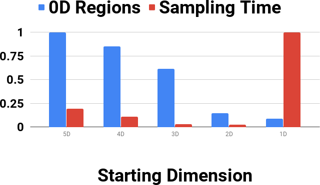
This experiment illustrates that when recursive search - starting from higher dimensional (energy) interior to lower dimensional boundary - is decoupled from sampling, it has a huge advantage over typical methods that remain in lower dimensional (energy) regions, validating the discussion in Section 3.3.1.
We use the EASAL software to enumerate all the lowest potential energy 0D regions in the assembly system with a pair of narrow concave (6 atoms) rigid molecular component as input. While EASAL typically starts sampling from the interior of 5D regions, in this experiment, we compare its time complexity and accuracy in discovering 0D regions to alternatively starting the sampling from the interior of 4D, 3D, 2D and 1D regions.
Figure 24 shows that when EASAL starts from 5D regions it discovers the most number of 0D regions and takes a reasonable amount of time. The number of 0D regions found decreases as the starting dimension for sampling decreases. The time required initially decreases with dimension as well, but dramatically increases, once the starting dimension decreases to a turning point. This is due to the combinatorial blow up of the number of possible starting regions, most of which do not have valid configurations, being low dimensional. Thus, starting from the interior of a higher dimensional (energy) region and recursively finding lower dimensional boundary regions is most effective at finding all minimum potential energy regions.
4.3.3 Region Specific Parametrization for Decoupling and Volumes
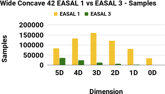
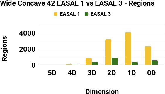
The results in this section demonstrate the advantages of region-specific parametrization both in finding active constraint regions and in computing volumes, validating the discussion in Section 3.5.1.
The first experiment quantifies the advantage of sampling each lower dimensional boundary region using a region-specific parametrization instead of just using a single parametrization of a region to sample its lower dimensional boundary regions.
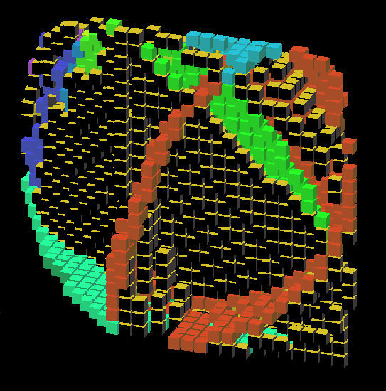
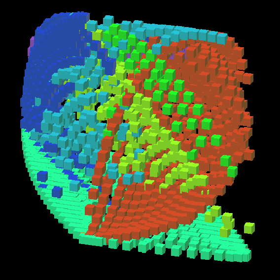
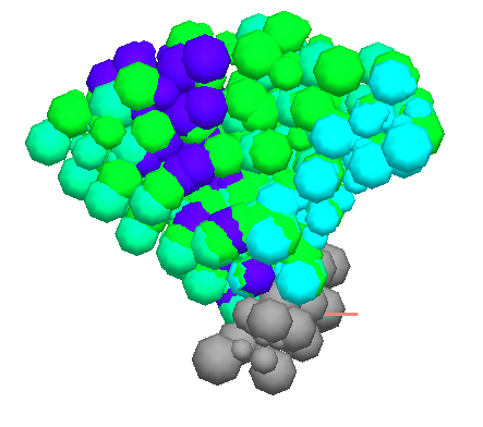
We sample the assembly landscape of the 42 atom concave system using two different methods with the same starting step size. The first method, EASAL-1 with region-specific parametrization, starts by sampling a 5D Cayley region. When a child region is discovered, it creates a different Cayley parametrization for the child region and recursively samples the child region until all its descendants are explored.
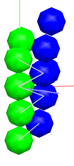
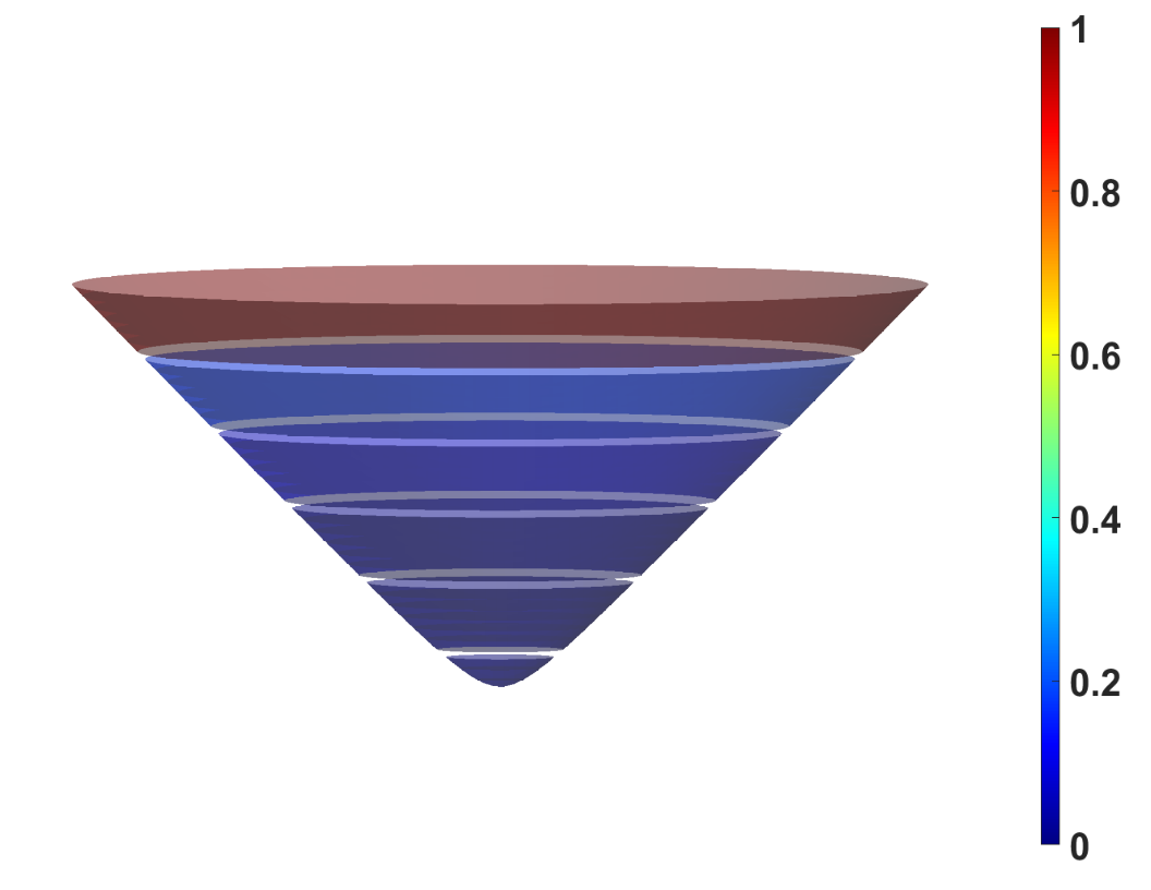
10pt23pt
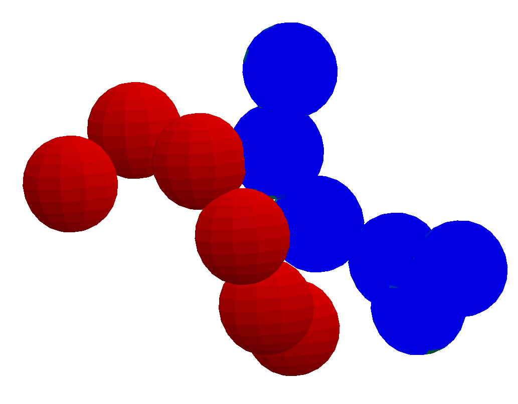
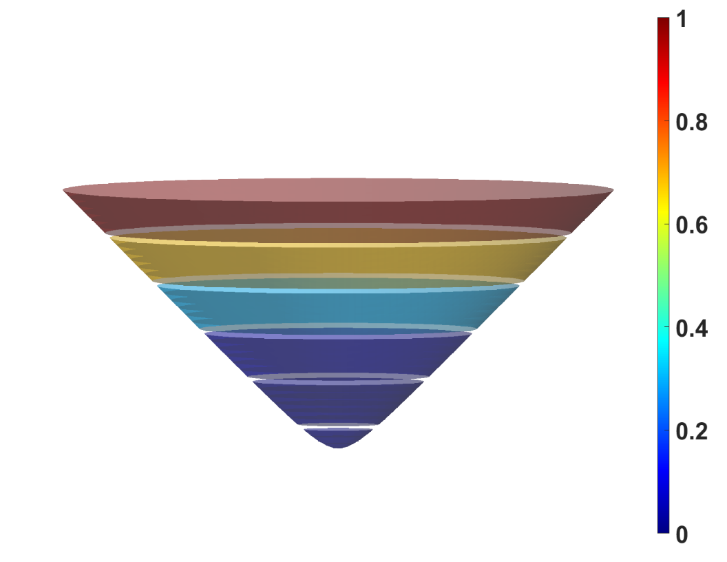
23pt43pt
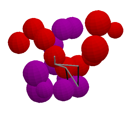
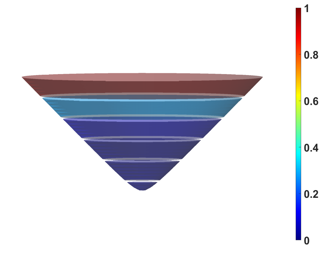
18pt33pt
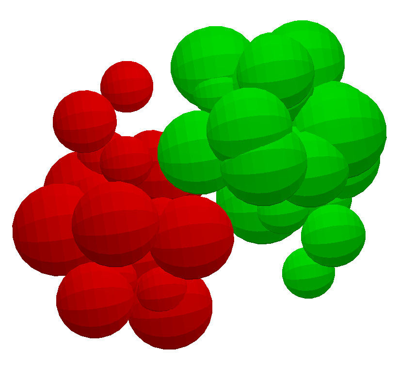
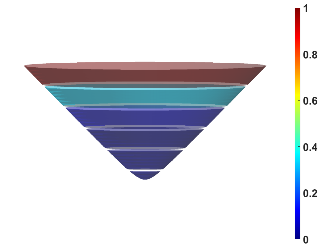
18pt38pt

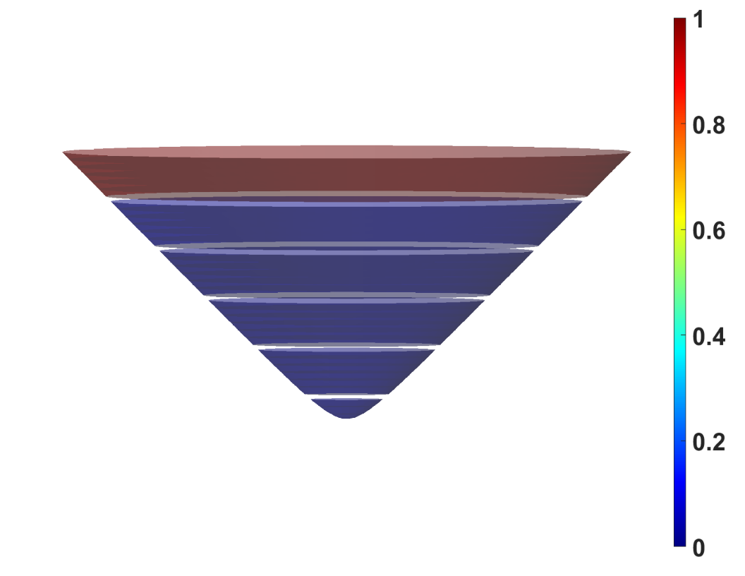
18pt38pt
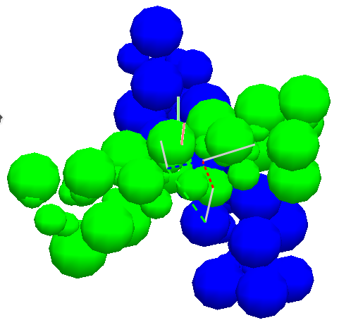
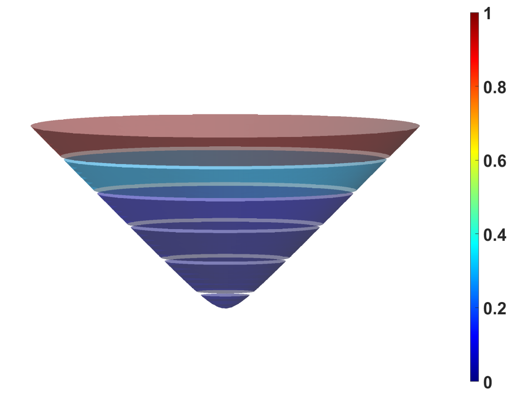
18pt33pt
The second method, EASAL-3 without region-specific parametrization, samples a 5D region densely close to the boundaries and sparsely in the interior, thereby sampling the descendant regions, in a single Cayley parametrization.
Figure 25 compares the number of regions and the number of samples found using the two methods. Figure 25 shows that EASAL-1 finds more configurations as compared to EASAL-3. In addition, Figure 25 shows that EASAL-1 finds more lower dimensional active constraint regions as well. Thus, region-specific parametrization further helps to decouple roadmap generation from sampling by reducing the number of samples required to find a given number of regions.
The second experiment shows that using region-specific parametrization provides better coverage sampling of active constraint regions. Figure 26 shows, using a concrete example in the EASAL software, how region-specific parametrization discovers more configurations.
4.4 Results on Volume Computation
| Rigid Molecular Component | Volume Computation Time (seconds) |
|---|---|
| 6 Convex | 1.4261 |
| 6 Concave | 4.4712 |
| 10 Concave | 9.0646 |
| 20 Convex | 22.6449 |
| 20 Concave | 20.1107 |
| 42 Concave | 106.8745 |
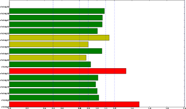
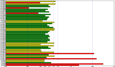
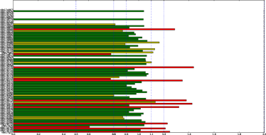
Results in this section demonstrate the performance of two algorithms for finding approximate and accurate volumes given in Sections 3.7.3 and 3.7.5.
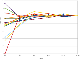
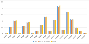
4.4.1 Approximate Basin Volume Computation
This experiment starts from a previously generated atlas and finds the volumes of potential energy basins extremely fast using the algorithm in Section 3.7.3. Results are tabulated in Table 4.
Figure 27 shows portions of the basin bar-codes, namely the weighted samples or approximate volumes stratified by dimension.
4.4.2 Comparison and Convergence of Entropy Integrals
This section demonstrates the performance of the algorithm in Section 3.7.5.
Figure 28 compares, for assembly systems with and identical spheres, 1D and 2D region integrals (See Equation (3) in Section 3.7.5) computed by our method to the results of the paper [47]. Already with coarse sampling, most of the ratios of values returned are in the range . Although some integrals differ by more than 50%, increasing sampling density has these integrals converge rapidly as shown in Figure 29(a).
The samples are uniformly distributed in Cayley region; the Jacobian relating Cayley to Cartesian parametrization (of Section 3.7.5) was not used to adjust either the sampling step size or direction, but only to scale the integral.
Our method extends to regions of any dimension. But since the paper [47] does not provide 3D region integrals we use two different methods to compute the integral and compare against each other.
The first ‘cell based’ method is the generalization of the 2D integral in 3D. At each grid point in Cayley region, the function value is computed and multiplied by the volume scaling factor calculated from the local Jacobian. The sum of this weighted function value at all the grid points is used as the numerical integral. By calculating the local numerical Jacobian we linearized the space locally, which could contribute to the error when the dimension is high and sampling is coarse.
The other “slice based” method is based on the integral of a 2D slice of the space. We partition the 3D Cayley region into a collection of 2D regions, or slices, by fixing one of the Cayley parameters. For each slice, the 2D integral is calculated as before. The sum of the slice integrals weighted by their thickness is used as the numerical 3D integral. The thickness for each 2D region is calculated as the average distance between neighboring slices. Our previous comparison shows that the error of local linearization is negligible for the 2D integral. So this result can be credibly used to check the magnitude of linearization error for the 3D integral.
Figure 29(b) shows the comparison between these two methods for all 3D regions of the assembly system with identical spheres. For the slice based method, we can partition the region in 3 different directions depending on the Cayley parameter to be fixed for each slice. So there are 3 different slice based results. As shown in the figure, the result from the 4 different methods are very similar, implying that the linearization error for the cell-based 3D integral is negligible.
4.5 Results on Verifying Time Complexity
We first demonstrate the performance of the core algorithm in Section 4.5.1 and in Section 4.5.2 we demonstrate the performance of the algorithm variant for and arbitrary .
4.5.1 Verifying the Core Algorithm’s Time Complexity
We demonstrate the performance of the core algorithm in Section 3.6.1 and verify the time complexity analysis in Section 3.6.3. Table 5 shows the sampling time, averaged across the 10 5D regions and their descendants for each of the 6 input rigid molecular component pairs, varying linearly in the number of weighted samples. As expected, the sampling time varies linearly in the number of regions but the factor of proportionality depends on the input rigid molecular component’s shape variables and is captured by the second landscape design variable as demonstrated in Section 4.2.2.
| Rigid Molecular Component | n | Regions | Weighted Samples | Sampling Time(seconds) |
|---|---|---|---|---|
| Narrow Convex | 6 | 3270 | 419k | 20 |
| Narrow Concave | 6 | 10128 | 2.2 million | 86 |
| Narrow Concave | 10 | 110554 | 11.5 million | 451 |
| Wide Convex | 20 | 112625 | 19.5 million | 1190 |
| Wide Concave | 20 | 63835 | 12.8 million | 775 |
| Wide Concave | 42 | 90190 | 31.5 million | 8580 |
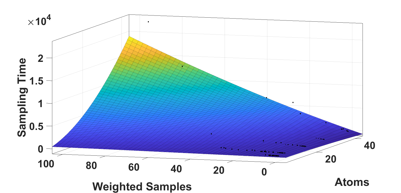
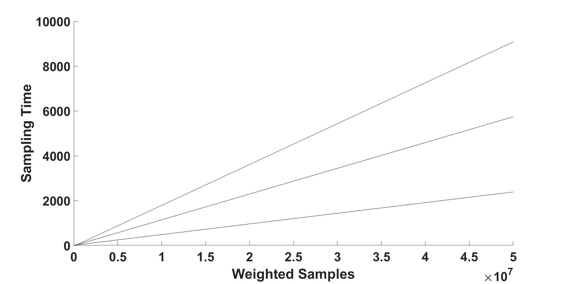
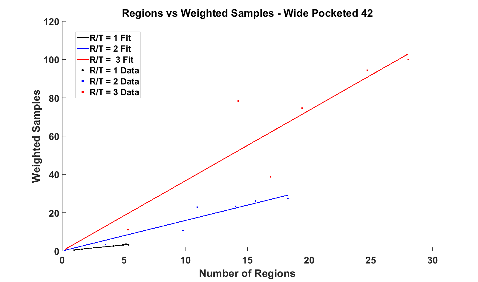
The next experiment verifies: (1) the expected linear dependence of sampling time on the number of weighted samples and quadratic dependence on the number of atoms (a constituent of the input shape variables); and (2) the influence of the sampling step size on the constant of proportionality between weighted samples and the number of regions.
Figure 30 plots the number of atoms and the number of weighted samples against the sampling time. Each point corresponds to a single run (using a 5D root node) described in Section 4.1.1. As expected, the plot also shows a bivariate function fit to this data using MATLAB conforming to a quadratic dependence on the number of atoms . Also as expected, slices of the function taken at different values of (see Figure 30) show a linear relationship between the number of weighted samples and the sampling time.
Figure 30 plots the number of samples against the number of regions for the wide concave rigid molecular component system (42 atoms). It shows three different lines, one each for the different step size. As can be seen from the plots, the slope of the line showing the number of samples against the number of regions, increases as the step size increases.
4.5.2 Verifying the Time Complexity of Algorithm Variant for arbitrary and
We demonstrate the performance of the second algorithm variant, described in Section 3.6.4, at atlasing the configuration space of the folding of the tryptophan zipper (trpzip 1). We decompose the tryptophan zipper into smaller rigid sub-units as described in [90, 91]. We use the benchmark data available at [92] as input and generate the topology of the landscape
The benchmark data for the tryptophan zipper consists as input a single molecule with 147 atoms divided into 17 groups of rigid sub-units, each varying in size from 4 atoms to 10 atoms. Using the second method in Section 3.6.4, we generate atlases with pairs of the rigid sub-units as input and give an estimate for the time required to find the complete atlas using this data.
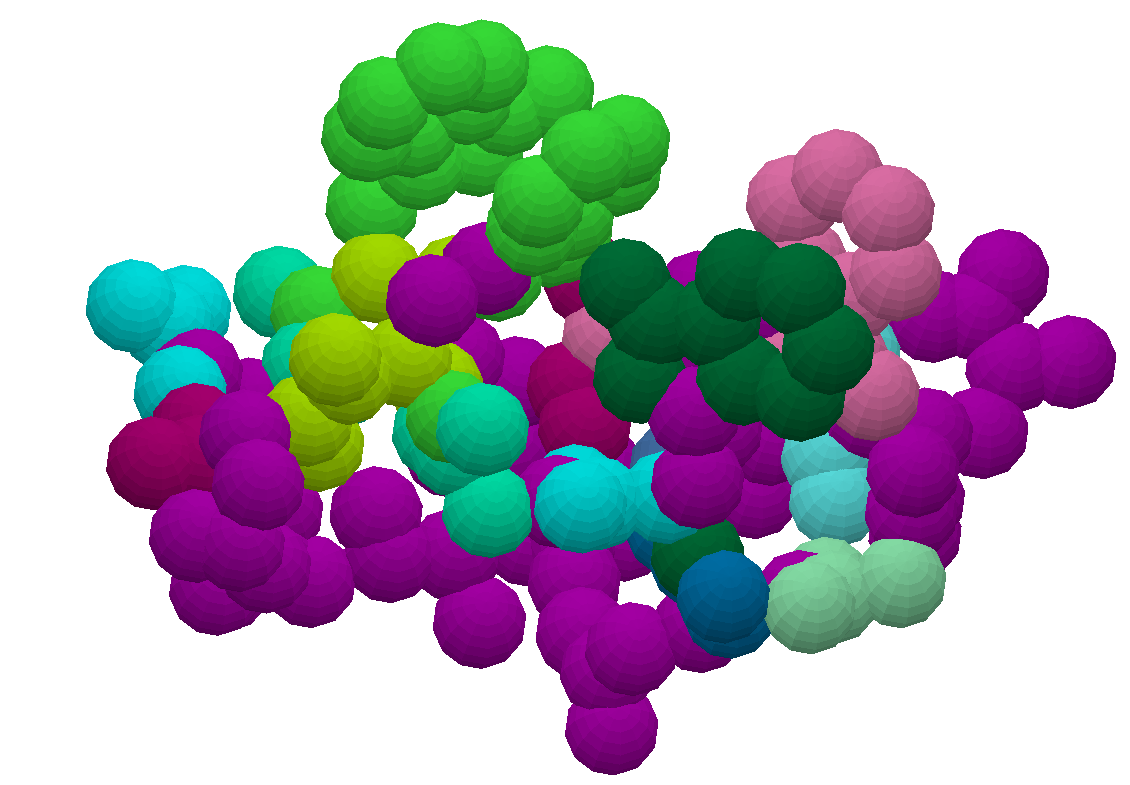
The output of the benchmark as described in the papers [93, 90] is a potential energy disconnectivity graph which, is gives information about all the minima in the landscape and the energy barriers separating them. The wealth of information in EASAL’s atlas subsumes this information. For example, the atlas provides the complete connectivity of basins, including all path lengths, basin volumes, and energy level information (see Figure 31 for an EASAL screenshot of a configuration in the folding landscape).
The following experiments were performed using the prototype parallel version of EASAL running on the hipergator supercomputer. We used 10 cores of Intel(R) Xeon(R) Gold 6142 CPU @ 2.60GHz processors and 10 GB of memory. Table 6 summarizes the atlasing time required by EASAL to generate the atlases of pairs of rigid molecular components in the first step. With these, we estimate the time required for the direct sum at each stage and finally the time required for generating the entire atlas.
| Rigid Molecular Components | Macrostates | Number of Energy Minima | Atlasing Time | Time per Minima |
|---|---|---|---|---|
| 10 - 10 | 2.6 million | 1.1 million | 6m 22s | 0.3 ms |
| 10 - 4 | 200k | 80k | 1m 30s | 1.1 ms |
| 4 - 4 | 7k | 2k | 50s | 25 ms |
Direct sum involves searching for active constraint regions of atlases. We assume a naive approach in the worst case, taking the direct sum at each internal node of the tree, which gives us a search time no worse than the product of the roadmap traversal time at the children. With more sophisticated techniques for direct sum (such as the one described in Section 3.6.4), we would in fact achieve significantly better search times, hence this is a conservative estimate. Next, we use the sampling time of the 10-10 pair at first level of the direct sum. Since most of the nodes at this level are of size 8 (4-4 pairs), this serves as a good approximation.
From Table 6, we estimate the search time for an atlas of size 10 as follows. On average, each node in the 10 atom atlas has 100 configurations, thus the time required to search for an active constraint region in the roadmap should be a hundredth of the time required to generate all the samples. In the case of the 10-10 molecular pair, this is 3.8 seconds. Propagating this product up the tree, we obtain a time of 12 hours at the root node to complete the process.
The number of energy minima at the root node can be estimated conservatively as in a similar way. Theoretically, every pair of minima at the child level produces a new minima at the parent node, but of these only a fraction are valid. Using the fraction we obtain from the 10-10 molecule (theoretical v/s observed), and propagating the number of minima up the tree, we get 5.8 billion minima in total at the root node, i.e., for the entire tryptophan zipper atlas. This gives us a sampling time per energy minimum of 7s.
5 Discussion
The new methodology presented in this paper combines many ideas e.g. geometrization, stratified roadmaps, recursive search. But the unique advantages (see Section 6 for a summary) can be traced directly or indirectly to the combination of these ideas with the use of Cayley parametrization to convexify constrained regions of the energy landscape that are topologically complex. Crucially, this parametrization permits traversal of the constrained region without having to explicitly enforce the constraints (which is usually done by minimizing constraint violation using gradient descent). Moreover, the convexity brings clear advantages in boundary detection, path and volume computations, ameliorating the curse of dimension. To the best of our knowledge, our methodology is the only one that uses this type of parametrization and convexification.
However, as pointed out, such convexification is only viable for active constraint graphs that occur in assembly, but not more generally in folding and other systems. Secondly, Cayley parameters are defined only for active constraint graphs, which in turn assume a pair-potential energy model that can be treated using geometric constraint systems. More global energy functions can be incorporated into the methodology, but not in ways that leverage Cayley parametrization. These represent inherent limits to extending the advantages of Cayley parametrization.
On the other hand, although the new methodology has not so far been leveraged beyond combining with standard multiscale techniques [77, 11], new methods are now being developed that transmit the unique strengths of Cayley parametrization across scales, e.g. in conjunction with the use of decomposition and recombination (DR) plans (as sketched in the core algorithm’s adaptation to large assemblies).
Overall, the new methodology can be used either as a resource-light, stand-alone method, or any combination of its features can be combined piecemeal with prevailing methods including MC and MD. Ongoing development of a parallel EASAL version, using the C++ Actor Framework (CAF) [94, 95], assigns different active constraint regions to different threads to sample in parallel, with one thread dedicated to keep track of the atlas. Results so far indicate no obstacles to linear speedup in the number of processors. This version would permit comparisons with other parallel methods [8, 57].
6 Conclusions
The paper has introduced a resource-light geometric method to generate and sample assembly landscapes characterized by short-range, Lennard-Jones pair potentials in an implicit solvent. The new methodology’s key strengths are robust and query-able generation of assembly landscape topology decoupled from sampling; intuitive design of landscapes using succinct bar-codes that connect input geometry with key landscape features; efficient sampling with refinable accuracy towards path and volume computations; and generalizability to a variety of assembly systems. Proof-of-concept results illustrating these features have been provided using a curated opensource software implementation [1].
The underlying theory is grounded in the classical concept of topological stratification and, more crucially, a recent understanding of convexification of configurational region using Cayley parameters. Consequently, the method provides quantifiable accuracy, isolation and coverage of narrow, low potential energy regions. Since the sampling is done by direct, region-specific parametrization that avoids the need to enforce constraints, it minimizes discarded samples and improves efficiency. Convexity additionally facilitates path finding, boundary detection, and volume computation even for high dimensional landscapes. While it can be used as a stand-alone method, its individual features can be hybridized with prevailing methods - with complementary strengths - promising an alternative approach to persistent computational challenges including free energy, configurational entropy, kinetics and multiscale modeling of significantly larger assemblies.
While the methodology formally characterizes and leverages the simplicity of assembly as opposed to folding, this also represents its inherent limits in that convex Cayley parametrization is only viable for assembly as opposed to folding or more general macromolecular energetic processes. Moreover the advantages of Cayley parametrization do not extend to more global energy functions that are not based on pair-potentials.
Acknowledgement
This research was supported in part by NSF Grants DMS-0714912, CCF-1117695, DMS-1563234, and DMS-1564480.
References
- [1] Aysegul Ozkan, Rahul Prabhu, Troy Baker, James Pence, Jorg Peters, and Meera Sitharam. Algorithm 990: Efficient atlasing and search of configuration spaces of point-sets constrained by distance intervals. ACM Trans. Math. Softw., 44(4):48:1–48:30, 2018.
- [2] Aysegul Ozkan, Rahul Prabhu, Troy Baker, James Pence, and Meera Sitharam. Efficient atlasing and search of assembly landscapes, 2016.
- [3] Rahul Prabhu, Troy Baker, and Meera Sitharam. Video illustrating the opensource software EASAL, 2016.
- [4] Rahul Prabhu and Meera Sitharam. EASAL software user guide., 2016.
- [5] Meera Sitharam, Audrey St. John, and Jessica Sidman. Handbook of Geometric Constraint Systems Principles. CRC Press, 1st edition, 2018.
- [6] Meera Sitharam and Heping Gao. Characterizing graphs with convex and connected cayley configuration spaces. Discrete & Computational Geometry, 43(3):594–625, 2010.
- [7] Samuel T. Chill, Jacob Stevenson, Victor Ruehle, Cheng Shang, Penghao Xiao, James D. Farrell, David J. Wales, and Graeme Henkelman. Benchmarks for characterization of minima, transition states, and pathways in atomic, molecular, and condensed matter systems. Journal of Chemical Theory and Computation, 10(12):5476–5482, 2014.
- [8] Deukhyun Cha, Qin Zhang, Jesmin Jahan Tithi, Alexander Rand, Rezaul A Chowdhury, and Chandrajit Bajaj. Accelerated molecular mechanical and solvation energetics on multicore cpus and manycore gpus. In Proceedings of the 6th ACM Conference on Bioinformatics, Computational Biology and Health Informatics, pages 222–231. ACM, 2015.
- [9] Meera Sitharam, Andrew Vince, Menghan Wang, and Miklós Bóna. Symmetry in sphere-based assembly configuration spaces. Symmetry, 8(1):5 1–26, 2016.
- [10] Ruijin Wu, Aysegul Ozkan, Antonette Bennett, Mavis Agbandje-Mckenna, and Meera Sitharam. Robustness measure for an adeno-associated viral shell self-assembly is accurately predicted by configuration space atlasing using easal. In Proceedings of the ACM Conference on Bioinformatics, Computational Biology and Biomedicine, BCB ’12, pages 690–695, New York, NY, USA, 2012. ACM.
- [11] Ruijin Wu, Rahul Prabhu, Antonette Bennett, Aysegul Ozkan, Mavis Agbandje-McKenna, and Meera Sitharam. Rapid prediction of crucial hotspot interactions for icosahedral viral capsid self-assembly by energy landscape atlasing validated by mutagenesis, 2020. arXiv:2001:00316.
- [12] Sergei Bespamyatnikh, Vicky Choi, Herbert Edelsbrunner, and Johannes Rudolph. Accurate protein docking by shape complementarity alone. Manuscript, Duke Univ., Durham, NC, 2004.
- [13] Vicky Choi, Pankaj K Agarwal, Herbert Edelsbrunner, and Johannes Rudolph. Local search heuristic for rigid protein docking. In International Workshop on Algorithms in Bioinformatics, pages 218–229, 2004.
- [14] E. Katchalski-Katzir, I. Shariv, M. Eisenstein, A. A. Friesem, C. Aflalo, and I. A. Vakser. Molecular surface recognition: determination of geometric fit between proteins and their ligands by correlation techniques. Proc. Natl. Acad. Sci. U.S.A., 89(6):2195–2199, Mar 1992.
- [15] Dina Duhovny, Ruth Nussinov, and Haim J Wolfson. Efficient unbound docking of rigid molecules. In International workshop on algorithms in bioinformatics, pages 185–200. Springer, 2002.
- [16] D. Schneidman-Duhovny, Y. Inbar, R. Nussinov, and H. J. Wolfson. PatchDock and SymmDock: servers for rigid and symmetric docking. Nucleic Acids Res., 33(Web Server issue):363–367, Jul 2005.
- [17] Ashini Bolia, Z. Nevin Gerek, and S. Banu Ozkan. Bp-dock: A flexible docking scheme for exploring protein-ligand interactions based on unbound structures. Journal of Chemical Information and Modeling, 54(3):913–925, 2014. PMID: 24380381.
- [18] Ashini Bolia and S. Banu Ozkan. Adaptive bp-dock: An induced fit docking approach for full receptor flexibility. Journal of Chemical Information and Modeling, 56(4):734–746, 2016. PMID: 26971620.
- [19] Pei Zhou, Botong Li, Yumeng Yan, Bowen Jin, Libang Wang, and Sheng-You Huang. Hierarchical flexible peptide docking by conformer generation and ensemble docking of peptides. Journal of Chemical Information and Modeling, 58(6):1292–1302, 2018. PMID: 29738247.
- [20] M. Karplus and J.N. Kushick. Method for estimating the configurational entropy of macromolecules. Macromolecules, 14(2):325–332, 1981.
- [21] Martha S Head, James A Given, and Michael K Gilson. Mining minima: Direct computation of conformational free energy. The Journal of Physical Chemistry A, 101(8):1609–1618, 1997.
- [22] IV Kurnikov, K Speranskiy, and MG Kurnikova. Harlem (hamiltonians to research large molecules). software package, 2001. https://crete.chem.cmu.edu/index.php/ software/harlem-software.
- [23] Ioan Andricioaei and Martin Karplus. On the calculation of entropy from covariance matrices of the atomic fluctuations. The Journal of Chemical Physics, 115(14):6289–6292, 2001.
- [24] Vladimir Hnizdo, Eva Darian, Adam Fedorowicz, Eugene Demchuk, Shengqiao Li, and Harshinder Singh. Nearest-neighbor nonparametric method for estimating the configurational entropy of complex molecules. Journal of Computational Chemistry, 28(3):655–668, 2007.
- [25] Benjamin J Killian, Joslyn Yundenfreund Kravitz, and Michael K Gilson. Extraction of configurational entropy from molecular simulations via an expansion approximation. The Journal of chemical physics, 127(2):024107–1 – 024107–16, 2007.
- [26] Vladimir Hnizdo, Jun Tan, Benjamin J Killian, and Michael K Gilson. Efficient calculation of configurational entropy from molecular simulations by combining the mutual-information expansion and nearest-neighbor methods. Journal of Computational Chemistry, 29(10):1605–1614, 2008.
- [27] Matthew Clark, Sia Meshkat, and Jeffrey S. Wiseman. Grand canonical free-energy calculations of protein-ligand binding. Journal of Chemical Information and Modeling, 49(4):934–943, 2009.
- [28] Matthew Clark, Siavash Meshkat, George T. Talbot, Paolo Carnevali, and Jeffrey S. Wiseman. Fragment-based computation of binding free energies by systematic sampling. Journal of Chemical Information and Modeling, 49(8):1901–1913, 2009. PMID: 19610599.
- [29] B. R. Brooks, C. L. Brooks III, A. D. Mackerell, L. Nilsson, R. J. Petrella, B. Roux, Y. Won, G. Archontis, C. Bartels, S. Boresch A. Caflisch, L. Caves, Q. Cui, A. R. Dinner, M. Feig, S. Fischer, J. Gao, M. Hodoscek, W. Im, K. Kuczera, T. Lazaridis, J. Ma, V. Ovchinnikov, E. Paci, R. W. Pastor, C. B. Post, J. Z. Pu, M. Schaefer, B. Tidor, R. M. Venable, H. L. Woodcock, X. Wu, W. Yang, D. M. York, , and M. Karplus. Charmm: the biomolecular simulation program. Journal of computational chemistry, 30(10):1545–1614, 2009.
- [30] Ulf Hensen, Oliver F Lange, and Helmut Grubmüller. Estimating absolute configurational entropies of macromolecules: The minimally coupled subspace approach. PLoS ONE, 5(2):1–8, 2010.
- [31] Gregory S. Chirikjian. Chapter four – modeling loop entropy. In Michael L. Johnson and Ludwig Brand, editors, Computer Methods Part C, volume 487 of Methods in Enzymology, pages 99 – 132. Academic Press, 2011.
- [32] Bracken M. King, Nathaniel W. Silver, and Bruce Tidor. Efficient calculation of molecular configurational entropies using an information theoretic approximation. The Journal of Physical Chemistry B, 116(9):2891–2904, 2012.
- [33] Chaitanya A. K. Koppisetty, Martin Frank, Graham J. L. Kemp, and Per-Georg Nyholm. Computation of binding energies including their enthalpy and entropy components for protein–ligand complexes using support vector machines. Journal of Chemical Information and Modeling, 53(10):2559–2570, 2013. PMID: 24050538.
- [34] D.A. Case, I.Y. Ben-Shalom, S.R. Brozell, D.S. Cerutti, T.E. Cheatham, III, V.W.D. Cruzeiro, T.A. Darden, R.E. Duke, D. Ghoreishi, M.K. Gilson, H. Gohlke, A.W. Goetz, D. Greene, R Harris, N. Homeyer, S. Izadi, A. Kovalenko, T. Kurtzman, T.S. Lee, S. LeGrand, P. Li, C. Lin, J. Liu, T. Luchko, R. Luo, D.J. Mermelstein, K.M. Merz, Y. Miao, G. Monard, C. Nguyen, H. Nguyen, I. Omelyan, A. Onufriev, F. Pan, R. Qi, D.R. Roe, A. Roitberg, C. Sagui, S. Schott-Verdugo, J. Shen, C.L. Simmerling, J. Smith, R. Salomon-Ferrer, J. Swails, R.C. Walker, J. Wang, H. Wei, R.M. Wolf, X. Wu, L. Xiao, D.M. York, and P.A. Kollman. Amber 18. Technical report, University of California, San Francisco, 2018.
- [35] Wei Jiang, Christophe Chipot, and Benoît Roux. Computing relative binding affinity of ligands to receptor: An effective hybrid single-dual-topology free-energy perturbation approach in namd. Journal of Chemical Information and Modeling, 59(9):3794–3802, 2019. PMID: 31411473.
- [36] Natalie Arkus, Vinothan Manoharan, and Michael Brenner. Minimal Energy Clusters of Hard Spheres with Short Range Attractions. Physical Review Letters, 103(11):118303 1–118303 4, 2009.
- [37] David J Wales. Energy landscapes of clusters bound by short-ranged potentials. Chemphyschem : a European journal of chemical physics and physical chemistry, 11(12):2491–2494, 2010.
- [38] Daniel J. Beltran-Villegas and Michael A. Bevan. Free energy landscapes for colloidal crystal assembly. Soft Matter, 7(7):3280–3285, 2011.
- [39] Florent Calvo, Jonathan P K Doye, and David J Wales. Energy landscapes of colloidal clusters: thermodynamics and rearrangement mechanisms. Nanoscale, 4(4):1085–1100, 2012.
- [40] Siddique J Khan, O L Weaver, C M Sorensen, and A Chakrabarti. Nucleation in short-range attractive colloids: ordering and symmetry of clusters. Langmuir : the ACS journal of surfaces and colloids, 28(46):16015–16021, 2012.
- [41] Robert S. Hoy, Jared Harwayne-Gidansky, and Corey S. O’Hern. Structure of finite sphere packings via exact enumeration: Implications for colloidal crystal nucleation. Physical Review E, 85(5):051403 1 – 051403 15, 2012.
- [42] Robert S. Hoy. Structure and dynamics of model colloidal clusters with short-range attractions. Phys. Rev. E, 91:012303 1 – 012303 7, 2015.
- [43] Jonathan P.K. Doye and David J. Wales. The structure of (C60)N clusters. Chemical Physics Letters, 262(1-2):167–174, 1996.
- [44] M. H. J. Hagen, E. J. Meijer, G. C. A. M. Mooij, D. Frenkel, and H. N. W. Lekkerkerker. Does C60 have a liquid phase? Nature, 365(6445):425–426, 1993.
- [45] Guangnan Meng, Natalie Arkus, Michael P. Brenner, and Vinothan N. Manoharan. The free-energy landscape of clusters of attractive hard spheres. Science (New York, N.Y.), 327(5965):560–563, 2010.
- [46] Domenico Gazzillo, Achille Giacometti, Riccardo Fantoni, and Peter Sollich. Multicomponent adhesive hard sphere models and short-ranged attractive interactions in colloidal or micellar solutions. Physical Review E, 74(5):051407 1–14, 2006.
- [47] Miranda Holmes-Cerfon, Steven J Gortler, and Michael P Brenner. A geometrical approach to computing free-energy landscapes from short-ranged potentials. Proceedings of the National Academy of Sciences of the United States of America, 110(1):E5–E14, 2013.
- [48] Lukas Trombach, Robert S. Hoy, David J. Wales, and Peter Schwerdtfeger. From sticky-hard-sphere to lennard-jones-type clusters. Phys. Rev. E, 97:043309 1–10, 2018.
- [49] Anthony Trubiano and Miranda Holmes-Cerfon. From canyons to valleys: Numerically continuing sticky-hard-sphere clusters to the landscapes of smoother potentials. Phys. Rev. E, 101:042608 1 – 13, Apr 2020.
- [50] David Gfeller, David Morton De Lachapelle, Paolo De Los Rios, Guido Caldarelli, and Francesco Rao. Uncovering the topology of configuration space networks. Physical Review E - Statistical, Nonlinear and Soft Matter Physics, 76(2 Pt 2):026113 1–9, 2007.
- [51] G Varadhan, Y J Kim, S Krishnan, and D Manocha. Topology preserving approximation of free configuration space. Robotics, (May):3041–3048, 2006.
- [52] Zaizhi Lai, Jiguo Su, Weizu Chen, and Cunxin Wang. Uncovering the properties of energy-weighted conformation space networks with a hydrophobic-hydrophilic model. International Journal of Molecular Sciences, 10(4):1808–1823, 2009.
- [53] Diego Prada-Gracia, Jesús Gómez-Garden̄es, Pablo Echenique, and Fernando Falo. Exploring the free energy landscape: From dynamics to networks and back. PLoS Comput Biol, 5(6):1–9, 2009.
- [54] Yuan Yao, Jian Sun, Xuhui Huang, Gregory R Bowman, Gurjeet Singh, Michael Lesnick, Leonidas J Guibas, Vijay S Pande, and Gunnar Carlsson. Topological methods for exploring low-density states in biomolecular folding pathways. The Journal of chemical physics, 130(14):144115 1–11, 2009.
- [55] David J. Wales. Surveying a complex potential energy landscape: Overcoming broken ergodicity using basin-sampling. Chemical Physics Letters, 584:1 – 9, 2013.
- [56] David J Earl and Michael W Deem. Parallel tempering: Theory, applications, and new perspectives. Physical Chemistry Chemical Physics, 7(23):3910–3916, 2005.
- [57] Matthew Griffiths and David J. Wales. Nested basin-sampling. Journal of Chemical Theory and Computation, 15(12):6865–6881, 2019.
- [58] David J. Wales. Exploring energy landscapes. Annual Review of Physical Chemistry, 69(1):401–425, 2018. PMID: 29677468.
- [59] John Canny. Computing roadmaps of general semi-algebraic sets. Computer Journal, 36:504–514, 1993.
- [60] J. Canny. A new algebraic method for robot motion planning and real geometry. In 28th Annual Symposium on Foundations of Computer Science (sfcs 1987), pages 39–48, 1987.
- [61] Saugata Basu, Richard Pollack, and Marie-Françoise Roy. Computing roadmaps of semi-algebraic sets on a variety. Journal of the American Mathematical Society, 13:55–82, 2000.
- [62] L. E. Kavraki, M. N. Kolountzakis, and J. C. Latombe. Analysis of probabilistic roadmaps for path planning. IEEE Transactions on Robotics and Automation, 14(1):166–171, 1998.
- [63] L. E. Kavraki, P. Svestka, J. C. Latombe, and M. H. Overmars. Probabilistic roadmaps for path planning in high-dimensional configuration spaces. IEEE Transactions on Robotics and Automation, 12(4):566–580, 1996.
- [64] Yuliy Baryshnikov, Peter Bubenik, and Matthew Kahle. Min-type morse theory for configuration spaces of hard spheres. International Mathematics Research Notices, 2014(9):2577–2592, 2014.
- [65] Matthew Kahle. Random geometric complexes. Discrete & Computational Geometry, 45(3):553–573, 2011.
- [66] Gunnar Carlsson, Jackson Gorham, Matthew Kahle, and Jeremy Mason. Computational topology for configuration spaces of hard disks. Phys. Rev. E, 85:011303 1–8, 2012.
- [67] Peter Bubenik, Gunnar Carlsson, Peter T Kim, and Zhi-Ming Luo. Statistical topology via morse theory persistence and nonparametric estimation. Algebraic methods in statistics and probability II, 516:75–92, 2010.
- [68] Matthew Kahle. Sparse locally-jammed disk packings. Annals of Combinatorics, 16(4):773–780, 2012.
- [69] Aleksandar Donev, Salvatore Torquato, Frank H. Stillinger, and Robert Connelly. Jamming in hard sphere and disk packings. Journal of Applied Physics, 95(3):989–999, 2004.
- [70] Léonard Jaillet and Josep M. Porta. Path Planning with Loop Closure Constraints Using an Atlas-Based RRT, pages 345–362. Springer International Publishing, Cham, 2017.
- [71] Emilio Zappa, Miranda Holmes-Cerfon, and Jonathan Goodman. Monte carlo on manifolds: Sampling densities and integrating functions. Communications on Pure and Applied Mathematics, 71(12):2609–2647, 2018.
- [72] Shawn Martin, Aidan Thompson, Evangelos A Coutsias, and Jean-Paul Watson. Topology of cyclo-octane energy landscape. The Journal of chemical physics, 132(23):234115 1–7, 2010.
- [73] Josep M Porta, Lluís Ros, Federico Thomas, Francesc Corcho, Josep Cantó, and Juan Jesús Pérez. Complete maps of molecular-loop conformational spaces. Journal of computational chemistry, 28(13):2170–2189, 2007.
- [74] Aaron R. Dinner, Erik Thiede, Brian Van Koten, and Jonathan Weare. Stratification as a general variance reduction method for markov chain monte carlo, 2017. arXiv:1705.08445.
- [75] Aysegul Ozkan and Meera Sitharam. Best of both worlds: Uniform sampling in cartesian and cayley molecular assembly configuration space. 2014. arXiv:1409.0956.
- [76] Aysegul Ozkan, Jose C. Flores-Canales, Meera Sitharam, and Maria Kurnikova. Fast and Flexible Geometric Method For Enhancing MC Sampling of Compact Configurations For Protein Docking Problem. 2014. arXiv:1408.2481.
- [77] Meera Sitharam. Modeling Autonomous Supramolecular Assembly, pages 197–216. Springer Berlin Heidelberg, Berlin, Heidelberg, 2014.
- [78] M. Sitharam and M. Agbandje-McKenna. Modeling virus assembly using geometric constraints and tensegrity:avoiding dynamics. 13(6):1232–1265, 2006. Journal of Computational Biology.
- [79] T Lazaridis and M Karplus. Effective energy function for proteins in solution. Proteins, 35(2):133–152, 1999.
- [80] Themis Lazaridis. Effective energy function for proteins in lipid membranes. Proteins, 52(2):176–192, 2003.
- [81] Wonpil Im, Michael Feig, and Charles L Brooks. An implicit membrane generalized born theory for the study of structure, stability, and interactions of membrane proteins. Biophysical Journal, 85(5):2900–2918, 2003.
- [82] Jack Graver, Brigitte Servatius, and Herman Servatius. Combinatorial Rigidity Graduate Studies in Mathematics, volume 2. American Mathematical Society, 1993.
- [83] Tzee-Char Kuo. On thom-whitney stratification theory. Mathematische Annalen, 234:97–107, 1978. 10.1007/BF01420960.
- [84] Robert Connelly, Steven J. Gortler, and Louis Theran. Rigidity for sticky discs. Proceedings of the Royal Society A: Mathematical, Physical and Engineering Sciences, 475(2222):20180773 1–16, 2019.
- [85] Wikipedia contributors. Covering space, 2020. [Online; accessed 3-July-2020].
- [86] Wikipedia contributors. Branched covering, 2020. [Online; accessed 3-July-2020].
- [87] Aysegul Ozkan and Meera Sitharam. Easal: Efficient atlasing, analysis and search of molecular assembly landscapes. In Proceedings of the ISCA 3rd International Conference on Bioinformatics and Computational Biology, BICoB-2011, pages 233–238, 2011.
- [88] Christoph M Hoffman, Andrew Lomonosov, and Meera Sitharam. Decomposition plans for geometric constraint systems, part i: Performance measures for cad. Journal of Symbolic Computation, 31(4):367–408, 2001.
- [89] C. M. Hoffmann, A. Lomonosov, and M. Sitharam. Decomposition of geometric constraints systems, part ii: new algorithms. Journal of Symbolic Computation, 31(4), 2001.
- [90] Jerelle A Joseph, Konstantin Röder, Debayan Chakraborty, Rosemary G Mantell, and David J Wales. Exploring biomolecular energy landscapes. Chemical Communications, 53(52):6974–6988, 2017.
- [91] Halim Kusumaatmaja, Chris S Whittleston, and David J Wales. A local rigid body framework for global optimization of biomolecules. Journal of chemical theory and computation, 8(12):5159–5165, 2012.
- [92] Gmin: A program for finding global minima and calculating thermodynamic properties from basin-sampling, 2020. Available Online : http://www-wales.ch.cam.ac.uk/examples/GMIN/.
- [93] Jerelle A. Joseph, Chris S. Whittleston, and David J. Wales. Structure, thermodynamics, and folding pathways for a tryptophan zipper as a function of local rigidification. Journal of Chemical Theory and Computation, 12(12):6109–6117, 2016. PMID: 27809512.
- [94] Dominik Charousset, Thomas C. Schmidt, Raphael Hiesgen, and Matthias Wählisch. Native Actors – A Scalable Software Platform for Distributed, Heterogeneous Environments. In Proc. of the 4rd ACM SIGPLAN Conference on Systems, Programming, and Applications (SPLASH ’13), Workshop AGERE, pages 87–96, New York, NY, USA, 2013. ACM.
- [95] Dominik Charousset, Raphael Hiesgen, and Thomas C. Schmidt. Revisiting Actor Programming in C++. Computer Languages, Systems & Structures, 45:105–131, 2016.
- [96] James Clerk Maxwell. On reciprocal figures and diagrams of forces. Philosophical Magazine, 27:250–261, 1864.
- [97] Ugandhar Reddy Chittamuru. Efficient bounds for 3d cayley configuration space of partial 2-trees. Master’s thesis, 2010.
Appendix
Appendix A Rigidity Preliminaries
The generic rigidity-based analysis of active constraint graphs in Section 3.2.1 uses the following concepts of combinatorial rigidity (we additionally refer the reader to the works [5, 82]). A (Euclidean) realization in of a graph , with edge lengths , is an assignment of points in to vertices such that the Euclidean distance between pairs of points are the given edge lengths (factoring out the Euclidean rigid body motions namely, the rotations and translations of ). A realization is said to be (locally) rigid if there is no other realization in its neighborhood that has the same edge lengths. A graph is said to be rigid if a generic realization of the graph with given edge lengths is rigid. Otherwise, the graph is said to be flexible (not rigid). A rigid graph, generically has finitely many realizations for a given set of edge lengths. A graph is said to be minimally rigid, well constrained or isostatic if it is rigid and the removal of any edge causes it to be flexible. All non-edges whose lengths are fixed by fixing the edge lengths of the graph, are (locally) implied or dependent.
The degrees of freedom (dof) of a graph is the minimum number of edges whose addition makes it rigid. Thus, the number of degrees of freedom is the same as the generic (effective) dimension of the realization space of the graph with given edge lengths. In , Maxwell’s theorem [96] states that if a graph is rigid, then there is a subset of edges , such that for every subset of vertices , , and . For , the right hand side is and for the right hand side is . The converse is true for , but fails for . A graph is independent if the removal of any edge increases the degrees of freedom. Thus, for an independent graph, the number of edges plus the number of degrees of freedom is .
Appendix B Cayley Convexification
We define a class of graphs that have a convex Cayley parametrization used in Section 3.4.1.
A complete 3-tree is any graph obtained by starting with a triangle and adding a new vertex adjacent to the vertices of a triangle in the current graph. Alternatively, this amounts to successively pasting a complete graph on 4 vertices (a tetrahedron) onto a triangle in the current graph. This yields a natural ordering of vertices in a 3-tree (we drop ‘complete’ when the context is clear). A 3-tree has edges and is minimally rigid in . Therefore, a 3-tree generically has finitely many realizations, and removing any edge gives a flexible partial 3-tree.
In , the analogous graphs for 3-trees are 2-trees. A complete 2-tree is any graph obtained by starting with an edge and successively pasting a triangle onto an edge in the current graph. A 2-tree is minimally rigid in and has edges. A partial 2-tree is any subgraph of complete 2-tree.
Theorem B.1 asserts that the length tuples of non-edges or Cayley parameters, - that complete a partial 3-tree into a 3-tree , or complete a partial 2-tree into a 2-tree - form a convex set (see the example in Section B.1). These length tuples are called Cayley configurations of the partial 3-tree . The chart for a graph and Cayley parameters is a map that takes a Cartesian realization of (with given edge lengths) to a Cayley configuration, i.e., the tuple of lengths of the non-edges in the Cartesian realization. The chart is a branched covering map. Therefore the theorem states that the chart for a partial 3-tree maps the set of Cartesian realizations of (given edge lengths or edge length intervals) to a convex set.
In addition to proving Theorem B.1, the paper [6] shows the existence of convex Cayley regions for a much larger class of graphs (beyond the scope of this paper).
Theorem B.1
Let the active constraint graph of a region be a partial 3-tree. Let be a set of non-edges such that is a 3-tree. Then the chart for with Cayley parameters maps the set of Cartesian realizations of (given edge lengths or edge length intervals) to a convex set. The convex set is bounded by polynomial inequalities (typically linear or quadratic). There is a sequence in which the parameters in can be fixed, such that the exact bounds on each successive parameter can be computed in time .
The quadratic and linear polynomials defined in Theorem B.1 arise from simple edge-length (metric) relationships in triangles and tetrahedra and are called triangle and tetrahedral inequalities. The exact bounds mentioned in the theorem are called tetrahedral bounds. The core algorithm of Section 3.6.1 leverages this efficient computation of the convex bounds enhanced by the Theorem 5.1.3 in the master’s thesis [97].
B.1 Example Toy2
Here, we use an active constraint graph in the assembly system of two molecules with 3 and 2 atoms respectively, to illustrate Cayley convexification in . Since that example is in , 2-trees (defined in Section B in the Appendix) serve the purpose of 3-trees used in our methodology [6].
Consider the partial 2-tree graph shown in Figure 32 (left). To represent the configurational region of this flexible graph, we add the non-edges and , shown with dotted lines, to complete the 2-tree. This not only makes the graph rigid, but finding its Cartesian configurations is easy by a straightforward ruler and compass construction, solving two quadratics at a time. The non-edges and are the Cayley parameters and correspond to independent flexes. Figure 32 shows the convex Cayley region corresponding to this graph.
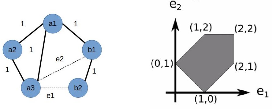
If the edges in the graph in Figure 32 (left) were assigned length intervals instead of fixed lengths, yielding an active constraint graph, the resulting configurational region would continue to be convex, but would be 7 dimensional. However, when these intervals are relatively small in comparison to the edge lengths, the Cayley region remains effectively 2 dimensional.
Furthermore, in the context of active constraint graphs, generalized 3-trees also yield convex Cayley parameters. This is because each rigid molecular component represents a unique realization of their underlying complete graph. A generalized 3-tree is defined by construction similar to a 3-tree. If 3 or more vertices in the already constructed graph belong to the same rigid molecular component , when a new vertex is added with edges to the vertices of a triangle in , then the vertices in can be replaced by any other distinct vertices in to which is adjacent. Moreover, generalized 3-trees, just like 3-trees, have an underlying sequence of tetrahedra, and are rigid with finitely many realizations. In this paper, we simply refer to generalized (partial) 3-trees as (partial) 3-trees.
Appendix C Cayley Configuration to Cartesian Configurations
Theorem C.1
In an assembly system with molecular units, each Cayley configuration corresponds to up to 8 Cartesian configurations.
Proof: Consider the first tetrahedron in a 3-tree completion of an active constraint graph that contains at least one edge (active constraint or Cayley parameter) between the two rigid molecular components and . The tetrahedron contains either (i) 2 vertices and in and 2 vertices , and in or without loss of generality (ii) 3 vertices , , and in and 1 vertex in . In either case the 3-tree will contain exactly 2 new (generalized) tetrahedra: In case (i) there are 4 edges between and and at most 2 further edges can be added to attain minimal rigidity. 2 additional (generalized) tetrahedra can be added: one with a vertex from and one with a vertex from distinct from . The vertex is connected by a new edge to or . The vertex is connected by a new edge to any vertex in . In case (ii) there are 3 edges between and and at most 3 further edges can be added to attain minimal rigidity. Again, 2 additional (generalized) tetrahedra can be added. The first containing and the second with . The vertex is connected to two of the vertices among , and the vertex is connected to any one of the vertices .
Appendix D Core Algorithm Details
This section details the core algorithm described briefly in Section 3.6.1. The exploration of the atlas is done by the recursive sampleAtlasNode algorithm using one of the generated atlas root nodes as input. Using depth first search, this algorithm samples the atlas node and all its descendants.
Base case of recursion: If active constraint graph of the node is minimally rigid i.e., the active constraint region is 0D, then there is only 1 Cayley configuration (with finitely many Cartesian configurations). We have no more sampling to do, hence return.
The recursion step: If is not minimally rigid, the core algorithm applies the complete3Tree algorithm to first check if is a partial 3-tree, and if so, find a set of non-edges that complete to a 3-tree. is the set of Cayley parameters. This leverages the convex parametrization theory [6] of Section 3.4 and additionally ensures that a graph with edge set is minimally rigid, and the corresponding Cartesian configurations can be easily found.
The computeConvexChart algorithm detects the tetrahedral bounds on these Cayley parameters as described below and samples uniformly within this region using a user specified step size.
-
•
If there is only one Cayley parameter in a tetrahedron, the tentative range of that parameter is computed by the intersection of tetrahedral inequalities.
-
•
If there is more than one unfixed Cayley parameter in a tetrahedron, then the tentative ranges of a parameters are computed in a specific sequence [97]. The tentative range of a parameter in the sequence is computed through tetrahedral inequalities using fixed values for the parameters appearing earlier in the sequence. Since the range of the parameter is affected by the previously fixed parameters, more precise range computation of the unfixed parameter is required for every iteration/assignment of fixed parameters.
Cayley Sampling Efficiency and Decoupling:
The actual range for each parameter for a given active constraint region is obtained by taking the intersection of
the tentative range and the range of Constraint . The order
in which Cayley parameters are fixed have an effect on the efficiency of the
range computation. We pick parameters in the order that gives
the best efficiency[97]. Once we choose the parameters and the sequence, the
explicit bounds can be computed in quadratic time in . Once explicit
bounds for each Cayley parameter have been found, we populate this region by
sampling it uniformly using a user specified step size. For roadmap generation,
coarse sampling is
sufficient since the boundary being detected is only one dimension less.
Robustness against coarse sampling is also provided by the
findAndSampleMissingAncestors algorithm, which ensures that all
for any non-empty active constraint region, all ancestor regions are
are added to the roadmap and sampled, even if they were initially missed
due to coarse sampling. This effectively
decouples roadmap generation from sampling.
Computing Cartesian Configurations:
For each Cayley configuration, the sampleAtlasNode algorithm computes its
Cartesian configurations using the computeRealization algorithm. The
computeRealization algorithm takes in a Cayley configuration and generates all
its 8 possible Cartesian configurations. There are 2 cases depending on
whether the active constraint graph is a partial 3-tree or not. Cartesian
configurations for partial 3-trees is straightforward as described in Section
3.4.2.
Boundary Detection:
After finding the Cartesian configurations, we perform the
aPosterioriConstraintViolated check to discover a boundary region.
This is the crucial test that indicates that a new constraint has become
active. The Cayley configuration, one of whose Cartesian configurations caused a child boundary region to
be found at a parent is called a witness point, since it witnesses the
boundary, and is placed in the child boundary region clearly labeled as a
witness point coming from each parent region.
The core algorithm relies on Cayley parameter grid sampling to find the child boundary regions of each active constraint region. However, boundary detection is not guaranteed by Cayley parameter grid sampling alone, since the sampling step size may be too large to identify a close-by atom pair that causes a constraint to become active. That is, the constraint violation could occur between 2 feasible sample realizations or between a feasible and an infeasible realization on the same flip in the sampling sequence. In the former case, the missed boundary region is “small,” and will later be discovered by the findAndSampleMissingAncestors. In the latter case, the newly active constraint has been flagged but exploration (by way of binary search) is required to find the exact Cayley parameter values at which new constraints became active. The binary search is on the Cayley parameter value, with direction determined by whether the realization is feasible or not.
Avoiding Repeat Sampling:
In both cases, once a new active constraint is discovered, we add the new
constraint to and create an new active constraint graph whose
edge set is . A boundary region could be detected via multiple parents.
However, since regions have unique labels, namely the active constraint graphs,
no region is sampled more than once. If has already been sampled, we just
add the node for into the atlas, as a child of . Otherwise, we create
a new atlas node with , sample it using the recursive
sampleAtlasNode algorithm and then add it as a child of .
Appendix E Symmetries in Assembly
This section discusses symmetries used in the algorithm variant described in Section 3.6.5. The concepts are developed in the paper [9]. An assembly configuration is an ordered set , where each , called a bunch, is a set of identical points. Two assembly configurations and are configurations of the same assembly system if is congruent to for some permutation , for all . The set of all assembly configurations of an assembly system is called an assembly configurational region.
Two assembly configurations and are isomorphic if there is a permutation such that for all , is isomorphic to . Two assembly configurations and are strictly isomorphic, if there is a permutation , such that for all , is isomorphic to . The weak automorphism group of is the group of all transformations that take to a strictly isomorphic . It is clear that all assembly configurations in the same assembly configurational region have the same weak automorphism group.
An active constraint graph of an assembly configuration is a graph where the vertex set has one vertex for each , and a vertex pair if and and are at a preferred distance from each other. Two active constraint graphs and are isomorphic if there is a such that . The automorphism group of an active constraint graph is the group of elements such that . This is also called the stabilizer group of . It is easy to see that the stabilizer group of is a subset of the stabilizer group of its active constraint graph . Figure 14 shows all the non-isomorphic active constraint graphs with 12 edges of an assembly system of 6 bunches each containing identical singleton spheres.
An active constraint region of the assembly configurational region contains all assembly configurations with active constraint graph .
Theorem E.1
[9] For an active constraint graph of an assembly configurational region , it holds that:
In addition, there exist active constraint graphs of assembly configurational region where the above containment is strict, i.e., for every such that ,
A fundamental domain of a stratification is the minimal sub-stratification such that , where each acts on via its action on the active constraint region of .