FERMILAB-CONF-12-065-E
CDF Note 10806
D0 Note 6303
Combined CDF and D0 Search for Standard Model Higgs Boson Production with up to 10.0 fb-1 of Data
Abstract
We combine results from CDF and D0 on direct searches for the standard model (SM) Higgs boson () in collisions at the Fermilab Tevatron at TeV. Compared to the previous Tevatron Higgs boson search combination more data have been added, additional channels have been incorporated, and some previously used channels have been reanalyzed to gain sensitivity. With up to 10 fb-1 of luminosity analyzed, the 95% C.L. median expected upper limits on Higgs boson production are factors of 0.94, 1.10, and 0.49 times the values of the SM cross section for Higgs bosons of mass 115 GeV/, 125 GeV/,and 165 GeV/, respectively. We exclude, at the 95% C.L., two regions: GeV/, and GeV/. We expect to exclude the regions GeV/ and GeV/. There is an excess of data events with respect to the background estimation in the mass range GeV/ which causes our limits to not be as stringent as expected. At GeV/, the -value for a background fluctuation to produce this excess is 3.510-3, corresponding to a local significance of 2.7 standard deviations. The global significance for such an excess anywhere in the full mass range is approximately 2.2 standard deviations. We also combine separately searches for and , and find that the excess is concentrated in the channel, although the results in the channel are also consistent with the possible presence of a low-mass Higgs boson.
Preliminary Results
I Introduction
Understanding the mechanism for electroweak symmetry breaking, specifically by testing for the presence or absence of the standard model (SM) Higgs boson, has been a major goal of particle physics for many years, and is a central part of the Fermilab Tevatron physics program. Both the CDF and D0 collaborations have performed new combinations CDFHiggs ; DZHiggs of multiple direct searches for the SM Higgs boson. The new searches include more data, additional channels, and improved analysis techniques compared to previous analyses. Precision electroweak data, including the recently updated measurements of the -boson mass from the CDF and D0 Collaborations CDFMW ; DZMW , yield an indirect constraint on the allowed mass of the Higgs boson, GeV/ lepewwg , at 95% confidence level (C.L.). The Large Electron Positron Collider (LEP) has excluded Higgs boson masses below 114.4 GeV/ lep , and the LHC experiments, ATLAS and CMS, now limit the SM Higgs boson to have a mass between 115.5 and 127 GeV/ atlas ; cms at the 95% C.L. Both LHC experiments report local standard deviation (s.d.) excesses at approximately 125 GeV/. The sensitivities of the new combinations presented here significantly exceeds those of previous Tevatron combinations prevhiggs ; WWPRLhiggs , providing sensitivity within the allowed Higgs boson mass range.
In this note, we combine the most recent results of all such searches in collisions at TeV in the Higgs boson mass range from 100–200 GeV/. The analyses combined here seek signals of Higgs bosons produced in association with a vector boson (), through gluon-gluon fusion (), and through vector boson fusion (VBF) () corresponding to integrated luminosities up to 10.0 fb-1 at CDF and up to 9.7 fb-1 at D0. The Higgs boson decay modes studied are , , , and . For Higgs boson masses greater than 125 GeV, modes with leptonic decay provide the greatest sensitivity keung ; glover ; hhg ; dittmar , while below 125 GeV sensitivity comes mainly from () where decays to and the or decays leptonically glashow ; marciano ; hhg . The dominant decay mode for a low mass Higgs boson is , and thus measurements of this process provide constraints on possible Higgs boson phenomenology that are complementary to those provided by the LHC.
To simplify the combination, the searches are separated into mutually exclusive final states referred to as “analysis sub-channels” in this note. Listings of these analysis sub-channels are provided in Tables 1 and 2. The selection procedures for each analysis are detailed in Refs. cdfWH through dzHgg , and are briefly described below.
II Acceptance, Backgrounds, and Luminosity
Event selections are similar for the corresponding CDF and D0 analyses, consisting typically of a preselection followed by the use of a multivariate analysis technique with a final discriminating variable to separate signal and background. For the case of , an isolated lepton ( electron or muon) and two or three jets are required, with one or more of the jets being -tagged, i.e., identified as containing a weakly-decaying hadron. Selected events must also display a significant imbalance in transverse momentum (referred to as missing transverse energy or ). Events with more than one isolated lepton are rejected.
For the D0 analyses, the data are split by lepton type and jet multiplicity (two or three jet sub-channels), and on the number of -tagged jets. Orthogonal selections corresponding to events with exactly one tight -tagged jet (TST), exactly two loose but not tight -tagged jets (LDT) and exactly two tight -tagged jets (TDT) are made. Every event is placed into one of these mutually exclusive categories. As with other D0 analyses targeting the decay, a boosted decision tree based -tagging algorithm, which builds and improves upon the previous neural network -tagger Abazov:2010ab , is used. For example, the loose -tagging criterion corresponds to an identification efficiency of for true -jets for a mis-identification rate of . The outputs of boosted decision trees, trained separately for each sample (i.e. jet multiplicity, lepton flavor and -tag category) and for each Higgs boson mass, are used as the final discriminating variables.
For the CDF analyses, events are analyzed in two and three jet sub-channels separately, and in each of these samples the events are grouped into various lepton and -tag categories. Events are broken into separate analysis categories based on the quality of the identified lepton. Separate categories are used for events with a high quality muon or central electron candidate, an isolated track or identified loose muon in the extended muon coverage, a forward electron candidate, and a loose central electron or isolated track candidate. The final two lepton categories, which provide some acceptance for lower quality electrons and single prong tau decays, are used only in the case of two-jet events. Within the lepton categories there are five -tagging categories considered for two-jet events: two tight -tags (TT), one tight -tag and one loose -tag (TL), a single tight -tag (Tx), two loose -tags (LL), and a single loose -tag. For three jet categories only the TT and TL -tagging categories are considered. The tight and loose -tag definitions are taken for the first time from a neural network tagging algorithm cdfHobit based on sets of kinematic variables sensitive to displaced decay vertices and tracks within jets with large transverse impact parameters relative to the hard-scatter vertices. Using an operating point which gives an equivalent rate of false tags, the new algorithm improves upon previous -tagging efficiencies by 20%. A Bayesian neural network discriminant is trained at each Higgs boson mass within the test range for each of the specific categories (defined by lepton type, -tagging type, and number of jets) to separate signal from backgrounds.
For the analyses, the selection is similar to the selection, except all events with isolated leptons are rejected and stronger multijet background suppression techniques are applied. Both the CDF and D0 analyses use a track-based missing transverse momentum calculation as a discriminant against false . In addition both CDF and D0 utilize multivariate techniques, a boosted decision tree at D0 and a neural network at CDF, to further discriminate against the multijet background before -tagging. There is a sizable fraction of the signal in which the lepton is undetected that is selected in the samples, so these analyses are also referred to as . The CDF analysis uses three non-overlapping categories of -tagged events (SS, SJ and 1S). These categories are based on two older CDF -tagging algorithms, an algorithm for reconstructing displaced, secondary vertices of -quark decays (S) and an algorithm for assigning a likelihood for tracks within a jet to have originated from a displaced vertex (J). The D0 analysis requires exactly two jets. The -tagging criteria have been re-optimized to reduce the loss in sensitivity due to systematic uncertainties. The tagger output values for each of the two jets are added to form an event -tag, the value of which is used to define two high purity samples: the medium -tag sample (MS) and the tight tag-sample (TS). After applying a multijet veto, these samples have a signal-to-background ratio of 0.3% and 1.5% respectively. Boosted decision trees, trained separately for the different -tagging categories and at each test mass, are used as the final discriminant. Overall, the sensitivity has been improved by 25% with respect to the previous result. The CDF analysis uses a second layer of neural network discriminants for separating signal from backgrounds.
The analyses require two isolated leptons and at least two jets. D0’s analyses separate events into non-overlapping samples of events with either one tight -tag (TST) or one tight and one loose -tag (TLDT). CDF has incorporated its new neural network -tagging algorithm in this analysis and uses four out of the five tagging categories (TT, TL, Tx, and LL). CDF now also separates events with two or three jets into independent analysis channels. To increase signal acceptance D0 loosens the selection criteria for one of the leptons to include an isolated track not reconstructed in the muon detector () or an electron from the inter-cryostat region of the D0 detector (). Combined with the dielectron () and dimuon () analyses, these provide four orthogonal analyses, and each uses 9.7 fb-1 of data in this combination. CDF uses neural networks to select loose dielectron and dimuon candidates. D0 applies a kinematic fit to optimize reconstruction, while CDF corrects jet energies for using a neural network approach. D0 uses random forests of decision trees to provide the final variables for setting limits. CDF utilizes a multi-layer discriminant based on neural networks where separate discriminant functions are used to define four separate regions of the final discriminant function.
For the analyses, signal events are characterized by large and two opposite-signed, isolated leptons. The presence of neutrinos in the final state prevents the accurate reconstruction of the candidate Higgs boson mass. D0 selects events containing electrons and/or muons, dividing the data sample into three final states: , , and . Each final state is further subdivided according to the number of jets in the event: 0, 1, or 2 or more (“2+”) jets. The dimuon and dielectron channels use boosted decision trees to reduce the dominant Drell-Yan background. Decays involving tau leptons are included in two orthogonal ways. A dedicated analysis () using 7.3 fb-1 of data studying the final state involving a muon and a hadronic tau decay plus up to one jet is included in the Tevatron combination. Final states involving other tau decays and mis-identified hadronic tau decays are included in the , , and final state analyses. CDF separates the events in five non-overlapping samples, split into “high ” and “low ” categories defined by lepton types and the number of reconstructed jets: 0, 1, or 2+ jets. The sample with two or more jets is not split into low and high lepton categories due to the smaller statistics in this channel. A sixth CDF channel is the low dilepton mass () channel, which accepts events with GeV. CDF has further improved its analysis of the low dilepton mass channel by reducing the cut applied to dilepton pairs down to 0.1, which increases Higgs signal acceptance in this channel 10%.
The division of events into categories based on the number of reconstructed jets allows the analysis discriminants to separate differing contributions of signal and background processes more effectively. The signal production mechanisms considered are , , and vector-boson fusion. The relative fractions of the contributions from each of the three signal processes and background processes, notably production and production, are very different in the different jet categories. Dividing our data into these categories provides more statistical discrimination, but introduces the need to evaluate the systematic uncertainties carefully in each jet category. A discussion of these uncertainties is found in Section III.
The D0 , , and final state channels use boosted decision trees as the final discriminants; for categories with non-zero jet multiplicity -tagging information is included. The channel uses neural networks as the final discriminant. CDF uses neural-network outputs, including likelihoods constructed from calculated matrix-element probabilities as additional inputs for the 0-jet bin.
D0 includes a analysis in which the associated vector boson and the boson from the Higgs boson decay are required to decay leptonically, giving like-sign dilepton final states. Previously the three final , , and were considered. In this combination, only the most sensitive final state is included. The combined output of two decision trees, trained against the instrumental and diboson backgrounds respectively, is used as the final discriminant. For the first time however, D0 includes tri-lepton analyses to increase the sensitivity to associated production and other decay modes, such as . The , and final states are considered. The and final states use boosted decision trees as the final discriminants. The final states are sub-divided according to the jet multiplicity to improve the sensitivity and a kinematic variable based on the event used as the discriminating variable.
CDF also includes a separate analysis of events with same-sign leptons to incorporate additional potential signal from associated production events in which the two leptons (one from the associated vector boson and one from a boson produced in the Higgs boson decay) have the same charge. CDF additionally incorporates three tri-lepton channels to include additional associated production contributions in which leptons result from the associated boson and the two bosons produced in the Higgs boson decay or where an associated boson decays into a dilepton pair and a third lepton is produced in the decay of either of the bosons resulting from the Higgs boson decay. In the latter case, CDF separates the sample into one jet and two or more jet sub-channels to take advantage of the fact that the Higgs boson candidate mass can be reconstructed from the invariant mass of the two jets, the lepton, and the missing transverse energy. CDF also includes for the first time a new tri-lepton channel focusing on production in which one of the three leptons is reconstructed as a hadronic tau.
CDF includes a search for using four lepton events. In addition to the simple four-lepton invariant mass discriminant used previously for separating potential Higgs boson signal events from the non-resonant background, the in these events is now used as a second discriminating variable to better identify four lepton signal contributions from and production. CDF has also updated its opposite-sign channels in which one of the two lepton candidates is a hadronic tau. Events are separated into - and - channels. The final discriminants are obtained from boosted decision trees which incorporate both hadronic tau identification and kinematic event variables as inputs.
D0 also includes channels in which one of the bosons in the process decays leptonically and the other decays hadronically. Electron and muon final states are studied separately. Random forests are used for the final discriminants.
CDF includes an updated, generic analysis searching for Higgs bosons decaying to tau lepton pairs incorporating contributions from direct production, associated or production, and vector boson fusion production. CDF also includes an analysis of events that contain one or more reconstructed leptons ( = or ) in addition to a tau lepton pair focusing on associated production where and additional leptons are produced in the decay of the or boson. For these searches multiple Support Vector Machine (SVM) svm classifiers are obtained using separate trainings for the signal against each of the primary backgrounds. In the generic search, events with either one or two jets are separated into two independent analysis channels. The final discriminant for setting limits is obtained using the minimum score of four SVM classifiers obtained from trainings against the primary backgrounds (, , multi-jet, and +jet production). In the extended analysis events are separated into five separate analysis channels (, , , , and ). The four lepton category includes candidates. The final discriminants are likelihoods based on outputs obtained from independent SVM trainings against each of the primary backgrounds (+jets, , and dibosons). These channels are included in the combination only for lower Higgs masses to avoid overlap with other search channels.
The D0 analyses likewise include direct production, associated or production, and vector boson fusion production. Decays of the Higgs boson to tau, and boson pairs are considered. A final state consisting of one leptonic tau decay, one hadronic tau decay and two jets is required. Both muonic and electronic sub-channels are considered. Recent improvements include increased trigger efficiencies. The output of boosted decision trees is used as the final discriminant.
CDF incorporates an updated all-hadronic analysis based on the older CDF -tagging algorithms, which results in two sub-channels (SS and SJ). Both and VBF production contribute to the final state. Events with either four or five reconstructed jets are selected, and at least two must be -tagged. The large QCD multijet backgrounds are modeled from the data by applying a measured mistag probability to the non -tagged jets in events containing a single -tag. Neural network discriminants based on kinematic event variables including those designed to separate quark and gluon jets are used to obtain the final limits.
D0 and CDF both contribute analyses searching for Higgs bosons decaying into diphoton pairs. The CDF analysis looks for a signal peak in the diphoton invariant mass spectrum above the smooth background originating from QCD production. Events are separated into four independent analysis channels based on the photon candidates contained within the event: two central candidates (CC), one central and one plug candidate (CP), one central and one central conversion candidate (C′C), or one plug and one central conversion candidate (C′P). In the D0 analysis the contribution of jets misidentified as photons is reduced by combining information sensitive to differences in the energy deposition from these particles in the tracker, calorimeter and central preshower in a neural network (ONN). The output of boosted decision trees, rather than the diphoton invariant mass, is used as the final discriminating variable. Previously, the transverse energies of the leading two photons along with the azimuthal opening angle between them and the diphoton invariant mass and transverse momentum were used as input variables. Additional variables, including the ONN output value for the two photons have been included, resulting in a sizeable improvement in sensitivity of .
CDF incorporates three non-overlapping sets of analysis channels searching for the process . One set of channels selects events with a reconstructed lepton, large missing transverse energy, and four or more reconstructed jets. Events containing four, five, and six or more jets are are analyzed separately and further sub-divided into five -tagging categories based on the older CDF tagging algorithms (three tight -tags (SSS), two tight and one loose -tags (SSJ), one tight and two loose -tags (SJJ), two tight -tags (SS), and one tight and one loose -tags (SJ)). Neural network discriminants trained at each mass point are used to set limits. A second set of channels selects events with no reconstructed lepton. These events are separated into two categories, one containing events with large missing transverse energy and five to nine reconstructed jets and another containing events with low missing transverse energy and seven to ten reconstructed jets. Events in these two channels are required to have a minimum of two -tagged jets based on an independent neural network tagging algorithm. Events with three or more -tags are analyzed in separate channels from those with exactly two tags. Two stages of neural network discriminants are used (the first to help reject large multijet backgrounds and the second to separate potential signal events from background events).
For both CDF and D0, events from QCD multijet (instrumental) backgrounds are typically measured in independent data samples using several different methods. For CDF, backgrounds from SM processes with electroweak gauge bosons or top quarks were generated using PYTHIA pythia , ALPGEN alpgen , MC@NLO MC@NLO , and HERWIG herwig programs. For D0, these backgrounds were generated using PYTHIA, ALPGEN, and COMPHEP comphep , with PYTHIA providing parton-showering and hadronization for all the generators. These background processes were normalized using either experimental data or next-to-leading order calculations (including MCFM mcfm for the heavy flavor process). All Monte Carlo samples are passed through detailed GEANT-based simulations geant of the CDF and D0 detectors.
Tables 1 and 2 summarize, for CDF and D0 respectively, the integrated luminosities, the Higgs boson mass ranges over which the searches are performed, and references to further details for each analysis.
| Channel | Luminosity | range | Reference |
| (fb-1) | (GeV/) | ||
| 2-jet channels 4(TT,TL,Tx,LL,Lx) | 9.45 | 100-150 | cdfWH |
| 3-jet channels 3(TT,TL) | 9.45 | 100-150 | cdfWH |
| (SS,SJ,1S) | 9.45 | 100-150 | cdfmetbb |
| 2-jet channels 2(TT,TL,Tx,LL) | 9.45 | 100-150 | cdfZH |
| 3-jet channels 2(TT,TL,Tx,LL) | 9.45 | 100-150 | cdfZH |
| 2(0 jets,1 jet)+(2 or more jets)+(low-) | 9.7 | 110-200 | cdfHWW |
| (-)+(-) | 9.7 | 130-200 | cdfHWW2 |
| (same-sign leptons)+(tri-leptons) | 9.7 | 110-200 | cdfHWW |
| tri-leptons with 1 | 9.7 | 130-200 | cdfHWW2 |
| (tri-leptons with 1 jet)+(tri-leptons with 2 or more jets) | 9.7 | 110-200 | cdfHWW |
| four leptons | 9.7 | 120-200 | cdfHZZ |
| + (1 jet)+(2 jets) | 8.3 | 100-150 | cdfHtt |
| / -- | 6.2 | 100-150 | cdfVHtt |
| / (--)+(--) | 6.2 | 100-125 | cdfVHtt |
| / -- | 6.2 | 100-105 | cdfVHtt |
| four leptons including candidates | 6.2 | 100-115 | cdfVHtt |
| (SS,SJ) | 9.45 | 100-150 | cdfjjbb |
| (CC,CP,CC-Conv,PC-Conv) | 10.0 | 100-150 | cdfHgg |
| (lepton) (4jet,5jet,6jet)(SSS,SSJ,SJJ,SS,SJ) | 9.45 | 100-150 | cdfttHLep |
| (no lepton) (low met,high met)(2 tags,3 or more tags) | 5.7 | 100-150 | cdfttHnoLep |
| Channel | Luminosity | range | Reference |
| (fb-1) | (GeV/) | ||
| (TST,LDT,TDT)(2,3 jet) | 9.7 | 100-150 | dzWHl |
| (MS,TS) | 9.5 | 100-150 | dzZHv2 |
| (TST,TLDT)(,,,) | 9.7 | 100-150 | dzZHll1 |
| + | 4.3-6.2 | 105-200 | dzVHt2 |
| 9.7 | 115-200 | dzWWW2 | |
| (0,1,2+ jet) | 8.6-9.7 | 115-200 | dzHWW |
| 7.3 | 115-200 | dzVHt2 | |
| 5.4 | 130-200 | dzHWWjj | |
| 9.7 | 100-200 | dzlll | |
| 7.0 | 115-200 | dzttl | |
| 9.7 | 100-150 | dzHgg |
III Signal Predictions
In order to predict the kinematic distributions of Higgs boson signal events, CDF and D0 use the PYTHIA pythia Monte Carlo program, with CTEQ5L and CTEQ6L1 cteq leading-order (LO) parton distribution functions. We scale these Monte Carlo predictions to the most recent higher-order calculations of inclusive cross sections, and differential cross sections, such as in the Higgs boson spectrum and the number of associated jets, as described below. The production cross section we use is calculated at next-to-next-to leading order (NNLO) in QCD with a next-to-next-to leading log (NNLL) resummation of soft gluons; the calculation also includes two-loop electroweak effects and handling of the running quark mass anastasiou ; grazzinideflorian . The numerical values in Table 3 are updates grazziniprivate of these predictions with set to 173.1 GeV/ tevtop09 , and with a treatment of the massive top and bottom loop corrections up to next-to-leading-order (NLO) + next-to-leading-log (NLL) accuracy. The factorization and renormalization scale choice for this calculation is . These calculations are refinements of the earlier NNLO calculations of the production cross section harlanderkilgore2002 ; anastasioumelnikov2002 ; ravindran2003 . Electroweak corrections were computed in Refs. actis2008 ; aglietti . Soft gluon resummation was introduced in the prediction of the production cross section in Ref. catani2003 . The production cross section depends strongly on the gluon parton density function, and the accompanying value of . The cross sections used here are calculated with the MSTW 2008 NNLO PDF set mstw2008 , as recommended by the PDF4LHC working group pdf4lhc . The inclusive Higgs boson production cross sections are listed in Table 3.
For analyses that consider inclusive production but do not split it into separate channels based on the number of reconstructed jets, we use the inclusive uncertainties from the simultaneous variation of the factorization and renormalization scale up and down by a factor of two. We use the prescription of the PDF4LHC working group for evaluating PDF uncertainties on the inclusive production cross section. QCD scale uncertainties that affect the cross section via their impacts on the PDFs are included as a correlated part of the total scale uncertainty. The remainder of the PDF uncertainty is treated as uncorrelated with the QCD scale uncertainty.
For analyses seeking production that divide events into categories based on the number of reconstructed jets, we employ a new approach for evaluating the impacts of the scale uncertainties. Following the recommendations of Ref. bnlaccord ; lhcdifferential , we treat the QCD scale uncertainties obtained from the NNLL inclusive grazzinideflorian ; anastasiou , NLO one or more jets anastasiouwebber , and NLO two or more jets campbellh2j cross section calculations as uncorrelated with one another. We then obtain QCD scale uncertainties for the exclusive jet, 1 jet, and 2 or more jet categories by propagating the uncertainties on the inclusive cross section predictions through the subtractions needed to predict the exclusive rates. For example, the +0 jet cross section is obtained by subtracting the NLO or more jet cross section from the inclusive NNLL+NNLO cross section. We now assign three separate, uncorrelated scale uncertainties which lead to correlated and anticorrelated uncertainty contributions between exclusive jet categories. The procedure in Ref. anastasiouwebber is used to determine PDF model uncertainties. These are obtained separately for each jet bin and treated as 100% correlated between jet bins and between D0 and CDF.
The scale choice affects the spectrum of the Higgs boson when produced in gluon-gluon fusion, and this effect changes the acceptance of the selection requirements and also the shapes of the distributions of the final discriminants. The effect of the acceptance change is included in the calculations of Ref. anastasiouwebber and Ref. campbellh2j , as the experimental requirements are simulated in these calculations. The effects on the final discriminant shapes are obtained by reweighting the spectrum of the Higgs boson production in the Monte Carlo simulations to higher-order calculations. The Monte Carlo signal simulation used by CDF and D0 is provided by the LO generator pythia pythia which includes a parton shower and fragmentation and hadronization models. We reweight the Higgs boson spectra in our pythia Monte Carlo samples to that predicted by hqt hqt when making predictions of differential distributions of signal events. To evaluate the impact of the scale uncertainty on our differential spectra, we use the resbos resbos generator, and apply the scale-dependent differences in the Higgs boson spectrum to the hqt prediction, and propagate these to our final discriminants as a systematic uncertainty on the shape, which is included in the calculation of the limits.
We include all significant Higgs boson production modes in the high-mass search. Besides gluon-gluon fusion through virtual quark loops (ggH), we include Higgs boson production in association with a or vector boson (VH), and vector boson fusion (VBF). For the low-mass searches, we target the , , VBF, and production modes with specific searches, including also those signal components not specifically targeted but which fall in the acceptance nonetheless. Our and cross sections are from Ref. djouadibaglio . This calculation starts with the NLO calculation of v2hv v2hv and includes NNLO QCD contributions vhnnloqcd , as well as one-loop electroweak corrections vhewcorr . A similar calculation of the cross section is available in Ref. grazziniferrera . We use the VBF cross section computed at NNLO in QCD in Ref. vbfnnlo . Electroweak corrections to the VBF production cross section are computed with the hawk program hawk , and are small and negative (2-3%) in the Higgs boson mass range considered here. We include these corrections in the VBF cross sections used for this result. The production cross sections we use are from Ref. tth .
The Higgs boson decay branching ratio predictions used for this result are those of Ref. lhcxs ; lhcdifferential . In this calculation, the partial decay widths for all Higgs boson decays except to pairs of and bosons are computed with HDECAY hdecay , and the and pair decay widths are computed with Prophecy4f prophecy4f . The relevant decay branching ratios are listed in Table 3. The uncertainties on the predicted branching ratios from uncertainties in , , , and missing higher-order effects are presented in Ref. dblittlelhc ; denner .
| (GeV/) | (fb) | (fb) | (fb) | (fb) | (fb) | (%) | (%) | (%) | (%) | (%) | (%) |
|---|---|---|---|---|---|---|---|---|---|---|---|
| 100 | 1821.8 | 281.1 | 162.7 | 97.3 | 8.0 | 79.1 | 3.68 | 8.36 | 1.11 | 0.113 | 0.159 |
| 105 | 1584.7 | 238.7 | 139.5 | 89.8 | 7.1 | 77.3 | 3.59 | 8.25 | 2.43 | 0.215 | 0.178 |
| 110 | 1385.0 | 203.7 | 120.2 | 82.8 | 6.2 | 74.5 | 3.46 | 8.03 | 4.82 | 0.439 | 0.197 |
| 115 | 1215.9 | 174.5 | 103.9 | 76.5 | 5.5 | 70.5 | 3.27 | 7.65 | 8.67 | 0.873 | 0.213 |
| 120 | 1072.3 | 150.1 | 90.2 | 70.7 | 4.9 | 64.9 | 3.01 | 7.11 | 14.3 | 1.60 | 0.225 |
| 125 | 949.3 | 129.5 | 78.5 | 65.3 | 4.3 | 57.8 | 2.68 | 6.37 | 21.6 | 2.67 | 0.230 |
| 130 | 842.9 | 112.0 | 68.5 | 60.5 | 3.8 | 49.4 | 2.29 | 5.49 | 30.5 | 4.02 | 0.226 |
| 135 | 750.8 | 97.2 | 60.0 | 56.0 | 3.3 | 40.4 | 1.87 | 4.52 | 40.3 | 5.51 | 0.214 |
| 140 | 670.6 | 84.6 | 52.7 | 51.9 | 2.9 | 31.4 | 1.46 | 3.54 | 50.4 | 6.92 | 0.194 |
| 145 | 600.6 | 73.7 | 46.3 | 48.0 | 2.6 | 23.1 | 1.07 | 2.62 | 60.3 | 7.96 | 0.168 |
| 150 | 539.1 | 64.4 | 40.8 | 44.5 | 2.3 | 15.7 | 0.725 | 1.79 | 69.9 | 8.28 | 0.137 |
| 155 | 484.0 | 56.2 | 35.9 | 41.3 | 2.0 | 9.18 | 0.425 | 1.06 | 79.6 | 7.36 | 0.100 |
| 160 | 432.3 | 48.5 | 31.4 | 38.2 | 1.8 | 3.44 | 0.159 | 0.397 | 90.9 | 4.16 | 0.0533 |
| 165 | 383.7 | 43.6 | 28.4 | 36.0 | 1.6 | 1.19 | 0.0549 | 0.138 | 96.0 | 2.22 | 0.0230 |
| 170 | 344.0 | 38.5 | 25.3 | 33.4 | 1.4 | 0.787 | 0.0364 | 0.0920 | 96.5 | 2.36 | 0.0158 |
| 175 | 309.7 | 34.0 | 22.5 | 31.0 | 1.3 | 0.612 | 0.0283 | 0.0719 | 95.8 | 3.23 | 0.0123 |
| 180 | 279.2 | 30.1 | 20.0 | 28.7 | 1.1 | 0.497 | 0.0230 | 0.0587 | 93.2 | 6.02 | 0.0102 |
| 185 | 252.1 | 26.9 | 17.9 | 26.9 | 1.0 | 0.385 | 0.0178 | 0.0457 | 84.4 | 15.0 | 0.00809 |
| 190 | 228.0 | 24.0 | 16.1 | 25.1 | 0.9 | 0.315 | 0.0146 | 0.0376 | 78.6 | 20.9 | 0.00674 |
| 195 | 207.2 | 21.4 | 14.4 | 23.3 | 0.8 | 0.270 | 0.0125 | 0.0324 | 75.7 | 23.9 | 0.00589 |
| 200 | 189.1 | 19.1 | 13.0 | 21.7 | 0.7 | 0.238 | 0.0110 | 0.0287 | 74.1 | 25.6 | 0.00526 |
IV Distributions of Candidates
All analyses provide binned histograms of the final discriminant variables for the signal and background predictions, itemized separately for each source, and the observed data. The number of channels combined is large, and the number of bins in each channel is large. Therefore, the task of assembling histograms and visually checking whether the expected and observed limits are consistent with the input predictions and observed data is difficult. We therefore provide histograms that aggregate all channels’ signal, background, and data together. In order to preserve most of the sensitivity gain that is achieved by the analyses by binning the data instead of collecting them all together and counting, we aggregate the data and predictions in narrow bins of signal-to-background ratio, . Data with similar may be added together with no loss in sensitivity, assuming similar systematic uncertainties on the predictions. The aggregate histograms do not show the effects of systematic uncertainties, but instead compare the data with the central predictions supplied by each analysis.
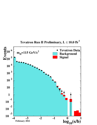
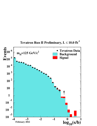
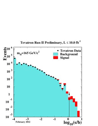
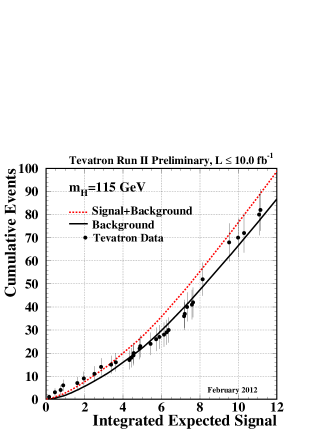
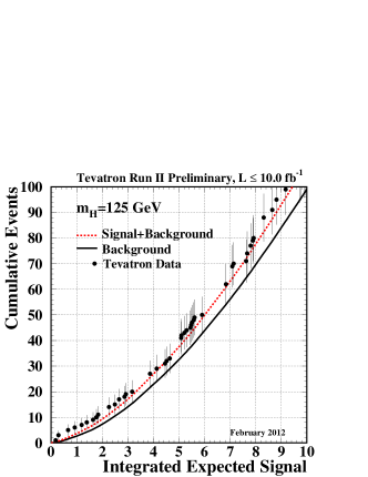
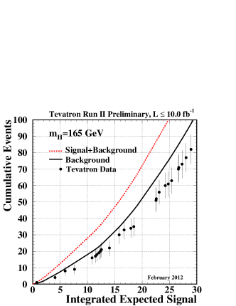
The range of is quite large in each analysis, and so is chosen as the plotting variable. Plots of the distributions of are shown for Higgs boson masses of 115, 125, and 165 GeV/ in Figure 1, demonstrating agreement with background over five orders of magnitude. These distributions can be integrated from the high- side downwards, showing the sums of signal, background, and data for the most pure portions of the selection of all channels added together. The integrals of the highest events are shown in Figure 2, plotted as functions of the number of signal events expected. The most significant candidates are found in the bins with the highest ; an excess in these bins relative to the background prediction drives the Higgs boson cross section limit upwards, while a deficit drives it downwards. The lower- bins show that the modeling of the rates and kinematic distributions of the backgrounds is very good. The integrated plots show an excess consistent with signal for the analyses seeking a Higgs boson mass of 125 GeV/, and a deficit of events in the highest- bins for the analyses seeking a Higgs boson of mass 165 GeV/.
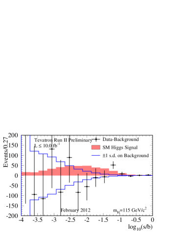
We also show the distributions of the data after subtracting the expected background, and compare that with the expected signal yield for a Standard Model Higgs boson, after collecting all bins in all channels sorted by . These background-subtracted distributions are shown in Figure 3 for Higgs boson masses of 115, 125, and 165 GeV/. These graphs also show the remaining uncertainty on the background prediction after fitting the background model to the data within the systematic uncertainties on the rates and shapes in each contributing channel.


V Combining Channels
To gain confidence that the final result does not depend on the details of the statistical formulation, we perform two types of combinations, using Bayesian and Modified Frequentist approaches, which yield limits on the Higgs boson production rate that agree within 10% at each value of , and within 1% on average. Both methods rely on distributions in the final discriminants, and not just on their single integrated values. Systematic uncertainties enter on the predicted number of signal and background events as well as on the distribution of the discriminants in each analysis (“shape uncertainties”). Both methods use likelihood calculations based on Poisson probabilities.
V.1 Bayesian Method
Because there is no experimental information on the production cross section for the Higgs boson, in the Bayesian technique CDFHiggs we assign a flat prior for the total number of selected Higgs boson events. For a given Higgs boson mass, the combined likelihood is a product of likelihoods for the individual channels, each of which is a product over histogram bins:
| (1) |
where the first product is over the number of channels (), and the second product is over histogram bins containing events, binned in ranges of the final discriminants used for individual analyses, such as the dijet mass, neural-network outputs, or matrix-element likelihoods. The parameters that contribute to the expected bin contents are for the channel and the histogram bin , where and represent the expected background and signal in the bin, and is a scaling factor applied to the signal to test the sensitivity level of the experiment. Truncated Gaussian priors are used for each of the nuisance parameters , which define the sensitivity of the predicted signal and background estimates to systematic uncertainties. These can take the form of uncertainties on overall rates, as well as the shapes of the distributions used for combination. These systematic uncertainties can be far larger than the expected SM Higgs boson signal, and are therefore important in the calculation of limits. The truncation is applied so that no prediction of any signal or background in any bin is negative. The posterior density function is then integrated over all parameters (including correlations) except for , and a 95% credibility level upper limit on is estimated by calculating the value of that corresponds to 95% of the area of the resulting distribution. This posterior density function may also be used to estimate the best-fit value of by finding that value which maximizes the posterior density. The fitted uncertainties are given by the shortest interval containing 68% of the integrated posterior density. These values are compared with those obtained from a profile likelihood fit to , maximizing over the values of the nuisance parameters, and give good agreement.
V.2 Modified Frequentist Method
The Modified Frequentist technique relies on the method, using a log-likelihood ratio (LLR) as test statistic DZHiggs :
| (2) |
where denotes the test hypothesis, which admits the presence of SM backgrounds and a Higgs boson signal, while is the null hypothesis, for only SM backgrounds and ’data’ is either an ensemble of pseudo-experiment data constructed from the expected signal and backgrounds, or the actual observed data. The probabilities are computed using the best-fit values of the nuisance parameters for each pseudo-experiment, separately for each of the two hypotheses, and include the Poisson probabilities of observing the data multiplied by Gaussian priors for the values of the nuisance parameters. This technique extends the LEP procedure pdgstats which does not involve a fit, in order to yield better sensitivity when expected signals are small and systematic uncertainties on backgrounds are large pflh .
The technique involves computing two -values, and . The latter is defined by
| (3) |
where is the value of the test statistic computed for the data. is the probability of observing a signal-plus-background-like outcome without the presence of signal, i.e. the probability that an upward fluctuation of the background provides a signal-plus-background-like response as observed in data. The other -value is defined by
| (4) |
and this corresponds to the probability of a downward fluctuation of the sum of signal and background in the data. A small value of reflects inconsistency with . It is also possible to have a downward fluctuation in data even in the absence of any signal, and a small value of is possible even if the expected signal is so small that it cannot be tested with the experiment. To minimize the possibility of excluding a signal to which there is insufficient sensitivity (an outcome expected 5% of the time at the 95% C.L., for full coverage), we use the quantity . If for a particular choice of , that hypothesis is deemed to be excluded at the 95% C.L. In an analogous way, the expected , and values are computed from the median of the LLR distribution for the background-only hypothesis.
Systematic uncertainties are included by fluctuating the predictions for signal and background rates in each bin of each histogram in a correlated way when generating the pseudo-experiments used to compute and .
An alternate computation of the -value is to use the fitted value of as a test statistic instead of LLR. This method is nearly as optimal as using LLR in our searches, and has been applied in the single top quark observation d0singletop . The background-only -value is the probability of obtaining the fitted cross section observed in the data or more, assuming that a signal is absent. We use this method to quote our -values and significances.
V.3 Systematic Uncertainties
Systematic uncertainties differ between experiments and analyses, and they affect the rates and shapes of the predicted signal and background in correlated ways. The combined results incorporate the sensitivity of predictions to values of nuisance parameters, and include correlations between rates and shapes, between signals and backgrounds, and between channels within experiments and between experiments. More on these issues can be found in the individual analysis notes cdfWH through dzHgg . Here we discuss only the largest contributions and correlations between and within the two experiments.
V.3.1 Correlated Systematics between CDF and D0
The uncertainties on the measurements of the integrated luminosities are 6% (CDF) and 6.1% (D0). Of these values, 4% arises from the uncertainty on the inelastic scattering cross section, which is correlated between CDF and D0. CDF and D0 also share the assumed values and uncertainties on the production cross sections for top-quark processes ( and single top) and for electroweak processes (, , and ). In order to provide a consistent combination, the values of these cross sections assumed in each analysis are brought into agreement. We use , following the calculation of Moch and Uwer mochuwer , assuming a top quark mass GeV/ tevtop09 , and using the MSTW2008nnlo PDF set mstw2008 . Other calculations of are similar otherttbar .
For single top, we use the next-to-next-to-next-to-leading-order (NNNLO) at next-to-leading logarithmic (NLL) -channel calculation of Kidonakis kid1 , which has been updated using the MSTW2008nnlo PDF set mstw2008 kidprivcomm . For the -channel process we use kid2 , again based on the MSTW2008nnlo PDF set. Both of the cross section values below are the sum of the single and single cross sections, and both assume GeV.
| (5) |
| (6) |
Other calculations of are similar for our purposes harris .
MCFM mcfm has been used to compute the NLO cross sections for , , and production dibo . Using a scale choice and the MSTW2008 PDF set mstw2008 , the cross section for inclusive production is
| (7) |
and the cross section for inclusive production is
| (8) |
The calculation is done using and therefore necessarily includes contributions from . The cross sections quoted above have the requirement GeV/ for the leptons from the neutral current exchange. The same dilepton invariant mass requirement is applied to both sets of leptons in determining the cross section which is
| (9) |
For the diboson cross section calculations, for all calculations. Loosening this requirement to include all leptons leads to +0.4% change in the predictions. Lowering the factorization and renormalization scales by a factor of two increases the cross section, and raising the scales by a factor of two decreases the cross section. The PDF uncertainty has the same fractional impact on the predicted cross section independent of the scale choice. All PDF uncertainties are computed as the quadrature sum of the twenty 68% C.L. eigenvectors provided with MSTW2008 (MSTW2008nlo68cl).
In many analyses, the dominant background yields are calibrated with data control samples. Since the methods of measuring the multijet (“QCD”) backgrounds differ between CDF and D0, and even between analyses within the collaborations, there is no correlation assumed between these rates. Similarly, the large uncertainties on the background rates for +heavy flavor (HF) and +heavy flavor are considered at this time to be uncorrelated. The calibrations of fake leptons, unvetoed conversions, -tag efficiencies and mistag rates are performed by each collaboration using independent data samples and methods, and are therefore also treated as uncorrelated.
V.3.2 Correlated Systematic Uncertainties for CDF
The dominant systematic uncertainties for the CDF analyses are shown in the Appendix in Tables 9 and 8 for the channels, in Table 12 for the channels, in Tables 14 and 15 for the channels, in Tables 17, 18, and 19 for the channels, in Table 20 for the and channels, in Table 21 for the channels, In Table 28 for the channel, in Tables 29, 30, and 31 for the channels, in Table 32 for the channels, in Table 33 for the and channels, in Table 34 for the and VBF channels, and in Table 35 for the channel. Each source induces a correlated uncertainty across all CDF channels’ signal and background contributions which are sensitive to that source. For , the largest uncertainties on signal arise from measured -tagging efficiencies, jet energy scale, and other Monte Carlo modeling. Shape dependencies of templates on jet energy scale, -tagging, and gluon radiation (“ISR” and “FSR”) are taken into account for some analyses (see tables). For , the largest uncertainties on signal acceptance originate from Monte Carlo modeling. Uncertainties on background event rates vary significantly for the different processes. The backgrounds with the largest systematic uncertainties are in general quite small. Such uncertainties are constrained by fits to the nuisance parameters, and they do not affect the result significantly. Because the largest background contributions are measured using data, these uncertainties are treated as uncorrelated for the channels. The differences in the resulting limits when treating the remaining uncertainties as either correlated or uncorrelated is less than .
V.3.3 Correlated Systematic Uncertainties for D0
The dominant systematic uncertainties for the D0 analyses are shown in the Appendix, in Tables 10, 11, 13, 16, 22, 23, 24, 26, 25, 27, and 36. Each source induces a correlated uncertainty across all D0 channels sensitive to that source. Wherever appropriate the impact of systematic effects on both the rate and shape of the predicted signal and background is included. For the low mass, analyses, significant sources of uncertainty include the measured -tagging rate and the normalization of the and plus heavy flavor backgrounds. For the and analyses, significant sources of uncertainty are the measured efficiencies for selecting leptons. For analyses involving jets the determination of the jet energy scale, jet resolution and the multijet background contribution are significant sources of uncertainty. Significant sources for all analyses are the uncertainties on the luminosity and the cross sections for the simulated backgrounds. All systematic uncertainties arising from the same source are taken to be correlated among the different backgrounds and between signal and background.
VI Combined Results
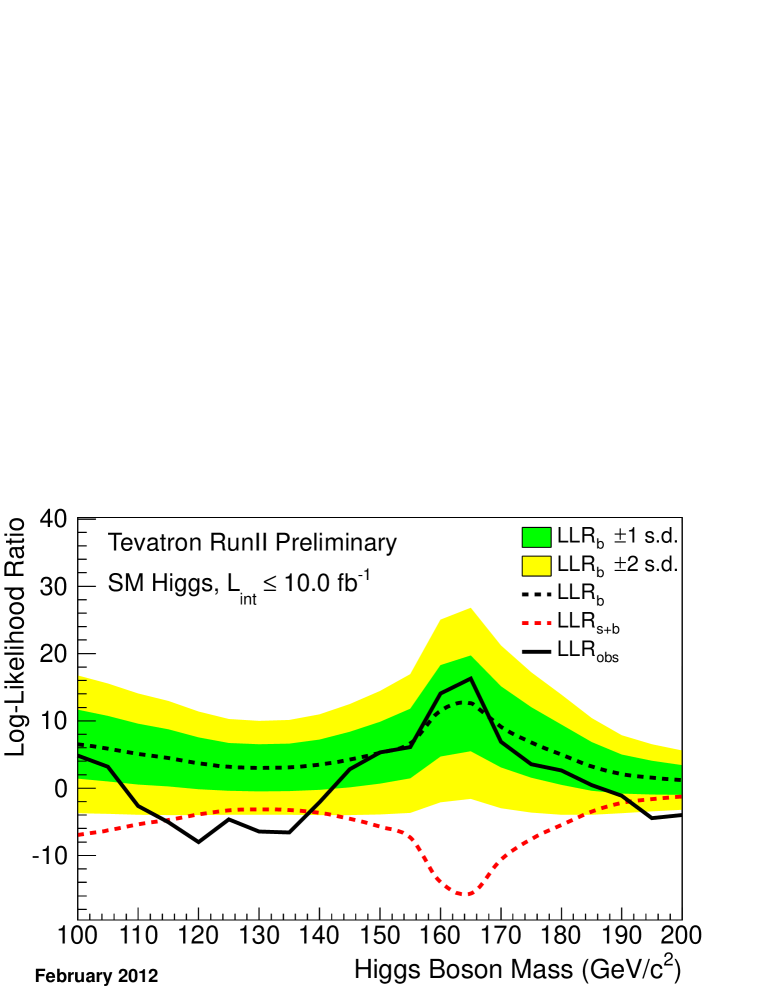
Before extracting the combined limits we study the distributions of the log-likelihood ratio (LLR) for different hypotheses to quantify the expected sensitivity across the mass range tested. Figure 4 and Table 6 display the LLR distributions for the combined analyses as functions of . Included are the median of the LLR distributions for the background-only hypothesis (LLRb), the signal-plus-background hypothesis (LLRs+b), and the observed value for the data (LLRobs). The shaded bands represent the one and two s.d. departures for LLRb centered on the median. The separation between the medians of the LLRb and LLRs+b distributions provides a measure of the discriminating power of the search. The sizes of the one- and two-s.d. LLRb bands indicate the width of the LLRb distribution, assuming no signal is truly present and only statistical fluctuations and systematic effects are present. The value of LLRobs relative to LLRs+b and LLRb indicates whether the data distribution appears to resemble what we expect if a signal is present (i.e. closer to the LLRs+b distribution, which is negative by construction) or whether it resembles the background expectation more closely; the significance of departures of LLRobs from LLRb can be evaluated by the width of the LLRb bands. The data are consistent with the prediction of the background-only hypothesis (the black dashed line) above 145 GeV/. For from 110 to 140 GeV/, an excess in the data has an amplitude consistent with the expectation for a standard model Higgs boson in this mass range (dashed red line). In this region our ability to distinguish the signal-plus-background and background-only hypotheses is, as indicated by the separation of the LLRs+b and LLRb values, at the 2 s.d. level.
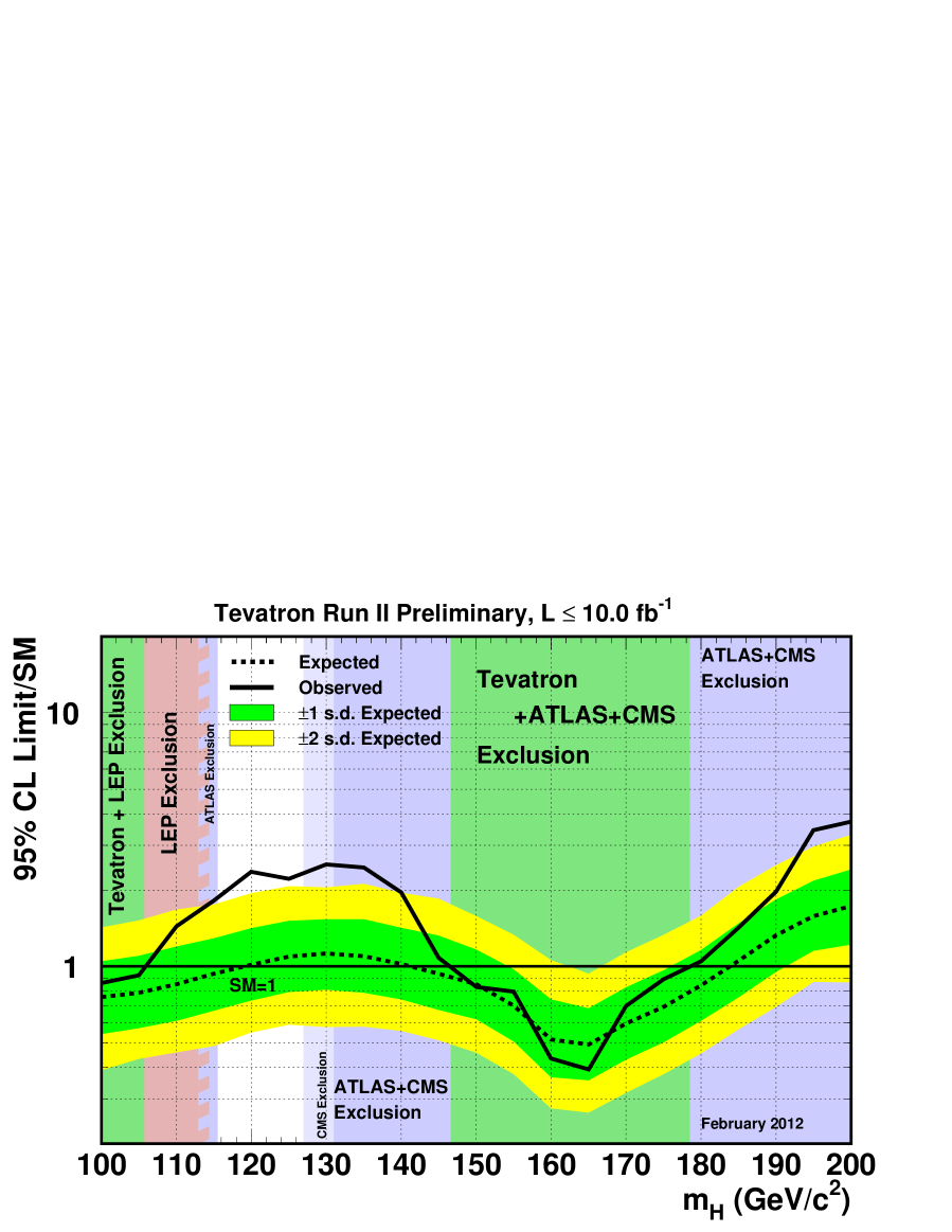
Using the combination procedures outlined in Section III, we extract limits on the SM Higgs boson production in collisions at TeV for GeV/. To facilitate comparisons with the standard model and to accommodate analyses with different degrees of sensitivity and acceptance for more than one signal production mechanism, we present our resulting limit divided by the SM Higgs boson production cross section, as a function of Higgs boson mass, for test masses for which both experiments have performed dedicated searches in different channels. A value of the combined limit ratio which is less than or equal to one indicates that that particular Higgs boson mass is excluded at the 95% C.L.
The combinations of results CDFHiggs ; DZHiggs of each single experiment, as used in this Tevatron combination, yield the following ratios of 95% C.L. observed (expected) limits to the SM cross section: 2.37 (1.16) for CDF and 2.17 (1.58) for D0 at GeV/, 2.90 (1.41) for CDF and 2.53 (1.85) for D0 at GeV/, and 0.42 (0.69) for CDF and 0.94 (0.76) for D0 at GeV/.
| Bayesian | 100 | 105 | 110 | 115 | 120 | 125 | 130 | 135 | 140 | 145 | 150 |
|---|---|---|---|---|---|---|---|---|---|---|---|
| Expected | 0.76 | 0.79 | 0.85 | 0.94 | 1.01 | 1.10 | 1.12 | 1.10 | 1.02 | 0.93 | 0.85 |
| Observed | 0.86 | 0.92 | 1.44 | 1.82 | 2.36 | 2.22 | 2.52 | 2.46 | 1.96 | 1.08 | 0.83 |
| 100 | 105 | 110 | 115 | 120 | 125 | 130 | 135 | 140 | 145 | 150 | |
| Expected | 0.76 | 0.80 | 0.86 | 0.92 | 1.02 | 1.11 | 1.13 | 1.12 | 1.05 | 0.95 | 0.84 |
| Observed | 0.84 | 0.97 | 1.52 | 1.88 | 2.20 | 2.23 | 2.65 | 2.62 | 1.93 | 1.07 | 0.83 |
| Bayesian | 155 | 160 | 165 | 170 | 175 | 180 | 185 | 190 | 195 | 200 |
|---|---|---|---|---|---|---|---|---|---|---|
| Expected | 0.70 | 0.52 | 0.49 | 0.60 | 0.69 | 0.84 | 1.05 | 1.33 | 1.58 | 1.73 |
| Observed | 0.80 | 0.43 | 0.39 | 0.70 | 0.89 | 1.05 | 1.42 | 1.97 | 3.45 | 3.73 |
| 155 | 160 | 165 | 170 | 175 | 180 | 185 | 190 | 195 | 200 | |
| Expected | 0.74 | 0.53 | 0.50 | 0.62 | 0.73 | 0.87 | 1.10 | 1.38 | 1.61 | 1.84 |
| Observed | 0.74 | 0.43 | 0.38 | 0.68 | 0.89 | 1.04 | 1.47 | 2.09 | 3.56 | 4.06 |
The ratios of the 95% C.L. expected and observed limit to the SM cross section are shown in Figure 5 for the combined CDF and D0 analyses. The observed and median expected ratios are listed for the tested Higgs boson masses in Table 4 for GeV/, and in Table 5 for GeV/, as obtained by the Bayesian and the methods. In the following summary we quote only the limits obtained with the Bayesian method, which was decided upon a priori. The corresponding limits and expected limits obtained using the method are shown alongside the Bayesian limits in the tables. We obtain the observed (expected) values of 0.92 (0.79) at GeV/, 1.82 (0.94) at GeV/, 2.22 (1.10) at GeV/, 1.08 (0.93) at GeV/, 0.39 (0.49) at GeV/, and 1.42 (1.05) at GeV/.
We choose to use the intersections of piecewise linear interpolations of our observed and expected rate limits in order to quote ranges of Higgs boson masses that are excluded and that are expected to be excluded. The sensitivities of our searches to Higgs bosons are smooth functions of the Higgs boson mass and depend most strongly on the predicted cross sections and the decay branching ratios (the decay is the dominant decay for the region of highest sensitivity). We therefore use the linear interpolations to extend the results from the 5 GeV/ mass grid investigated to points in between. The regions of Higgs boson masses excluded at the 95% C.L. thus obtained are GeV/ and GeV/. The expected exclusion regions are, given the current sensitivity, GeV/ and GeV/. Higgs boson masses below 100 GeV/ were not studied. We also show in Figure 6, and list in Table 7, the observed values of 1- and their expected distributions for the background-only hypothesis as functions of the Higgs boson mass. The excluded regions obtained by finding the intersections of the linear interpolations of the observed curve are nearly identical to those obtained with the Bayesian calculation.
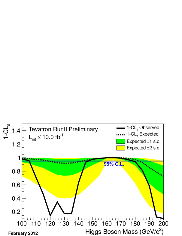
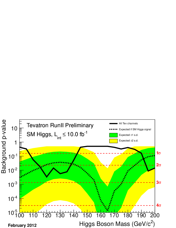
Figure 7 shows the -value as a function of as well as the expected distributions in the absence of a Higgs boson signal. Figure 8 shows the -value 1- as a function of , i.e., the probability that an upward fluctuation of the background can give an outcome as signal-like as the data or more. In the absence of a Higgs boson signal, the observed -value is expected to be uniformly distributed between 0 and 1. A small -value indicates that the data are not easily explained by the background-only hypothesis, and that the data prefer the signal-plus-background prediction. Our sensitivity to a Higgs boson with a mass of 165 GeV/ is such that we would expect to see a -value corresponding to s.d. in half of the experimental outcomes. The smallest observed -value corresponds to a Higgs boson mass of 120 GeV/. The fluctuations seen in the observed -value as a function of the tested result from excesses seen in different search channels, as well as from point-to-point fluctuations due to the separate discriminants at each , and are discussed in more detail below. The width of the dip in the -values from 115 to 135 GeV/ is consistent with the resolution of the combination of the and channels. The effective resolution of this search comes from two independent sources of information. The reconstructed candidate masses help constrain , but more importantly, the expected cross sections times the relevant branching ratios for the and channels are strong functions of in the SM. The observed excesses in the channels coupled with a more background-like outcome in the channels determines the shape of the observed -value as a function of .
We perform a fit of the signal-plus-background hypothesis to the observed data, allowing the signal strength to vary as a function of . The resulting best-fit signal strength is shown in Figure 9, normalized to the SM prediction. The signal strength is within 1 s.d. of the SM expectation with a Higgs boson signal in the range GeV. The largest signal fit in this range, normalized to the SM prediction, is obtained at 130 GeV. The reason the highest signal strength is at 130 GeV/ while the smallest -value from Figure 8 is at 120 GeV is because a signal at 120 GeV would have a higher cross section than a signal at 130 GeV, and since the resolution of the discriminants cannot distinguish very well such a small mass difference, a signal at 120 GeV would be similar to a signal at 130 GeV with a larger scale factor for the predicted cross section.
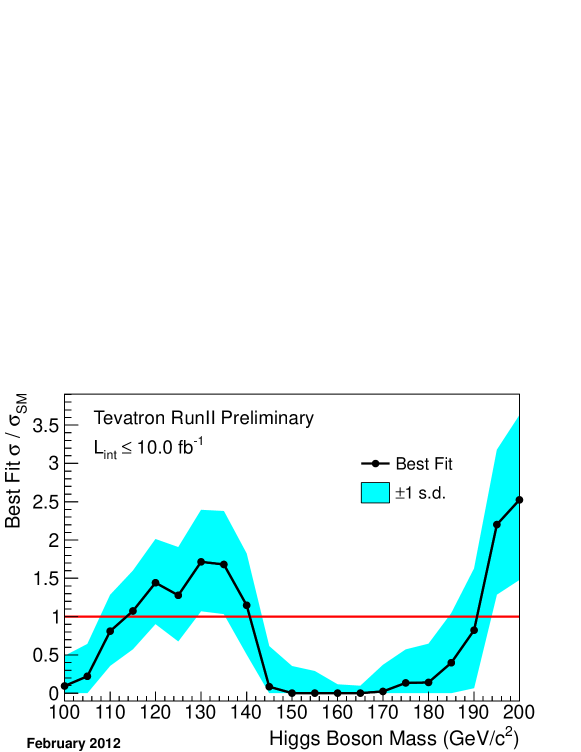
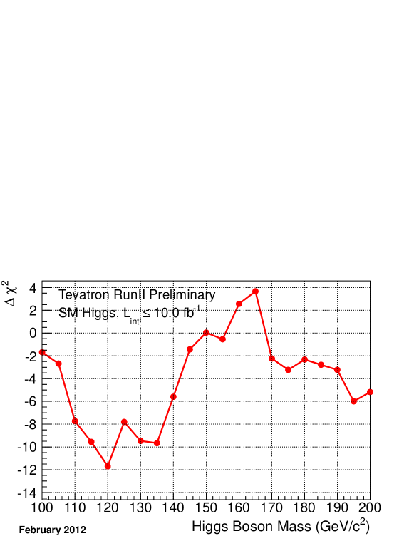
Figure 10 shows , which is an estimate of how discrepant the observed data are with the median expectation from the prediction of the background-only hypothesis, as a function of . Significantly negative values of indicate a preference in the data for the signature of Higgs boson production.
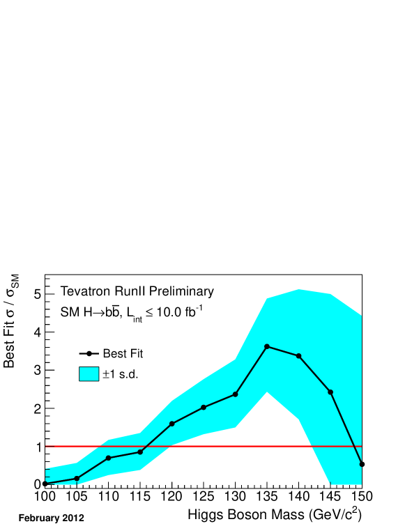
We also investigate combinations of CDF and D0 searches based on the and decay modes. Below 125 GeV/, the searches contribute the majority of our sensitivity. The , , and channels from both experiments are included in this combination. The result is shown in Figure 11. The distribution of the LLR demonstrates the compatibility of the observed data with both the background-only and signal-plus-background hypotheses, and is shown in Figure 12. An interesting feature of this graph is that as increases towards the high end of the range shown, falls rapidly, and the expected signal yield becomes small. Thus LLR approaches zero as gets larger, independent of the experimental outcome. This feature can also be seen with the shaded bands which also converge on zero at high . If there is a broad excess in the searches, then LLR will fall to a minimum value and rise again.
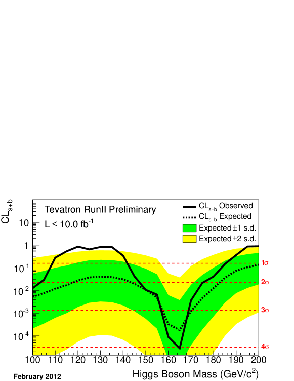
Figure 13 shows the observed and expected values of CLs+b as functions of mH. Figure 14 shows the -value for the background-only hypothesis 1 - CLb, which represents the probability for the background to fluctuate to produce an outcome as signal-like as the observed data or more. The smallest -value within the mass range where these searches are performed, GeV/, corresponds to a significance of approximately 2.8 s.d.
These probabilities do not include the look-elsewhere effect (LEE), and are thus local -values, corresponding to searches at each value of separately. The LEE accounts for the probability of observing an upwards fluctuation of the background at any of the tested values of in our search region, at least as significant as the one observed at the value of with the most significant local excess. A simple and correct method of calculating the LEE, and thus the global significance of the excess, is to simulate many possible experimental outcomes assuming the absence of a signal, and for each one, compute the LLR and the fitted cross section curves and find the deviation with the smallest background-only-hypothesis -value. Using this minimum -value as a test statistic, another -value is then computed, which is the probability of observing that minimum -value or less. This method is difficult to pursue in the Tevatron Higgs boson searches due to the fact that in most search analyses, a distinct multivariate analysis (MVA) discriminant function is trained for each value of that is tested. This step is an important optimization, because the kinematic distributions and signal branching ratios are functions of , but it introduces the difficulty of running the same set of simulated events separately through many MVA functions in order to compute the LEE with the simple method. The use of a separate MVA function at each also introduces additional point-to-point randomness as individual events are reclassified from bins with lower to higher and vice versa. Even though the discriminants are nearly optimal and are thus highly similar from one value to the next, small variations are amplified by the discrete nature of the data which are processed through these MVAs. One may see this in the variations of observed limits, LLR values and -values from one mass point to the next which show more rapid variation than can be explained from mass resolution effects alone.
Gross and Vitells grossvitells provide a technique that extrapolates from a smaller sample of background-only Monte Carlo simulations fully propagated through the MVA discriminant functions. We lack the ability to perform this propagation through all of our channels, as we rely on exchanged histograms of distributions of selected events. We therefore estimate the LEE effect in a simplified manner. In the mass range 100–130 GeV, where the low-mass searches dominate, the reconstructed mass resolution is approximately 10-15%, or about 15 GeV. We therefore estimate a LEE factor of for the low-mass region. The searches have a much better mass resolution, of order 3%, but their contribution to the final LLR is small due to the much smaller in those searches. They introduce more rapid oscillations of LLR as a function of , but the magnitude of these oscillations is much smaller than those induced by the searches. The searches have both worse reconstructed mass resolution and lower than the searches and therefore similarly do not play a significant role in the estimation of the LEE. Applying the LEE of 2 to the most significant local -value obtained from our combination, we obtain a global significance of approximately 2.6 s.d.
We perform a fit of the signal-plus-background hypothesis to the observed data, allowing the signal strength to vary as a function of . The resulting best-fit signal strength is shown in Figure 15, normalized to the SM prediction. The excess comes mainly from the CDF channels, which have combined s.d. excesses, with the most signal-like candidates coming from CDF’s channel. The , , and search channels all contribute to the increase in significance of the CDF excess with respect to previous combinations. The larger excesses found in each individual channel are consistent with the large numbers of new events being added to the searches through the analysis of new data and use of the improved neural-network -tagging algorithm. For the channel, which sees the largest change in the significance of its observed excess, more than half of the currently analyzed data events were not contained within previous analyses of this channel. The D0 channels see a 1 s.d. excess, consistent with the signal-plus-background hypothesis.
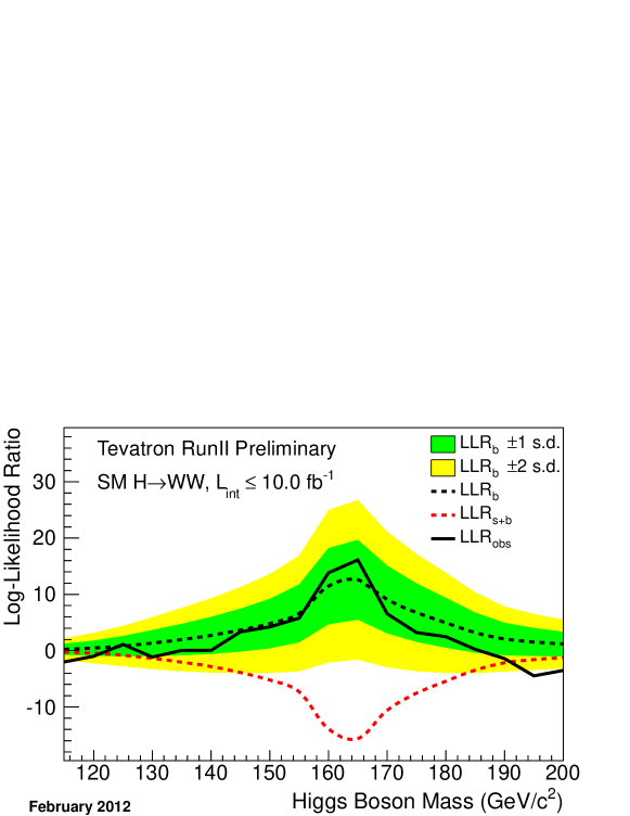
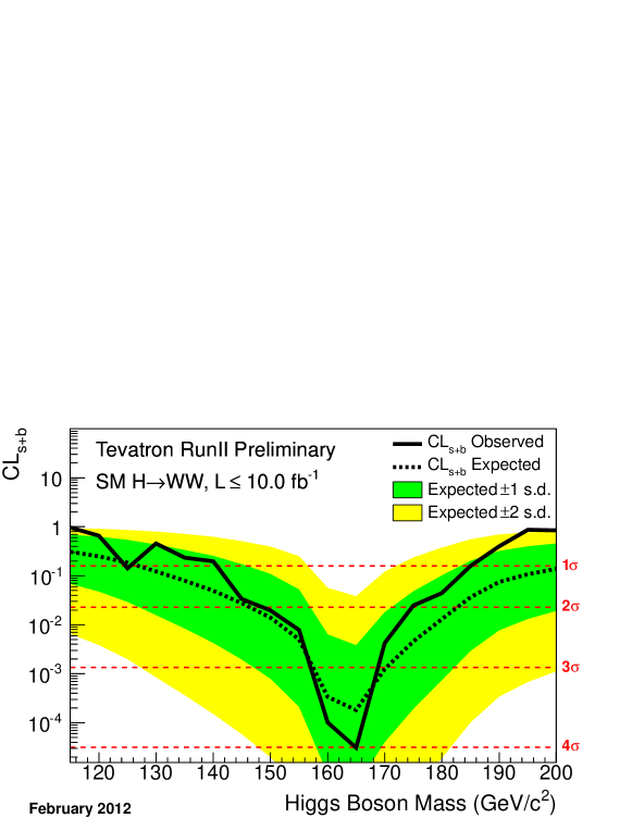
Above 125 GeV/, the channels contribute the majority of our search sensitivity. We combine all searches from CDF and D0, incorporating potential signal contributions from , , , and VBF production. The result of this combination is shown in Figure 16. The distribution of the LLR is shown in Figure 17, which shows good agreement overall with the background-only hypothesis. Where the sensitivity is low, for GeV/ and 190 GeV/, the data are slightly more compatible with the signal-plus-background hypothesis. Figure 18 shows the observed and expected CLs+b distribution as a function of mH. Figure 19 shows the -value for the background-only hypothesis. We perform a fit of the observed data to the signal-plus-background hypothesis, allowing the signal strength to vary in the fit as a function of as shown in Figure 20. Consistent with Figure 17 the combined observed data do not indicate any significant excesses, though the D0 analysis has a slight excess ( s.d.) from 130 to 140 GeV/ consistent with the signal-plus-background hypothesis.
The analyses which dominate the sensitivity of our high mass searches have poor resolution for reconstructing due to the presence of two neutrinos in the final states of the most sensitive channels, and we thus expect the outcomes in these searches at each in the high-mass range to be highly correlated with each other. Above , the bosons are on shell, and the kinematic variables take on different weights in the training of the MVAs than they do at masses below . At very high masses, the discriminating variable cdfHWW ; dzHWW plays less of a role than it does near the threshold. We therefore expect a LEE factor of approximately two for our high-mass searches in the mass range 130 200 GeV/. Over the entire mass range of our Higgs searches, 100 200 GeV/, we therefore expect that there are roughly four possible independent locations for uncorrelated excesses to appear in our analysis. The global -value associated with our entire suite of Higgs searches is therefore , using the Dunn-Ŝidák correction dunn . Based on this approach, if we simply chose to consider the region not currently excluded by other experiments, our resulting LEE factor would be one, making the global significance equivalent to the local significance. The smallest local -value obtained from the full combination of CDF and D0 SM Higgs searches has a significance of approximately 2.7 s.d. Applying a LEE of 4 to this value, we obtain a global significance of approximately 2.2 s.d.
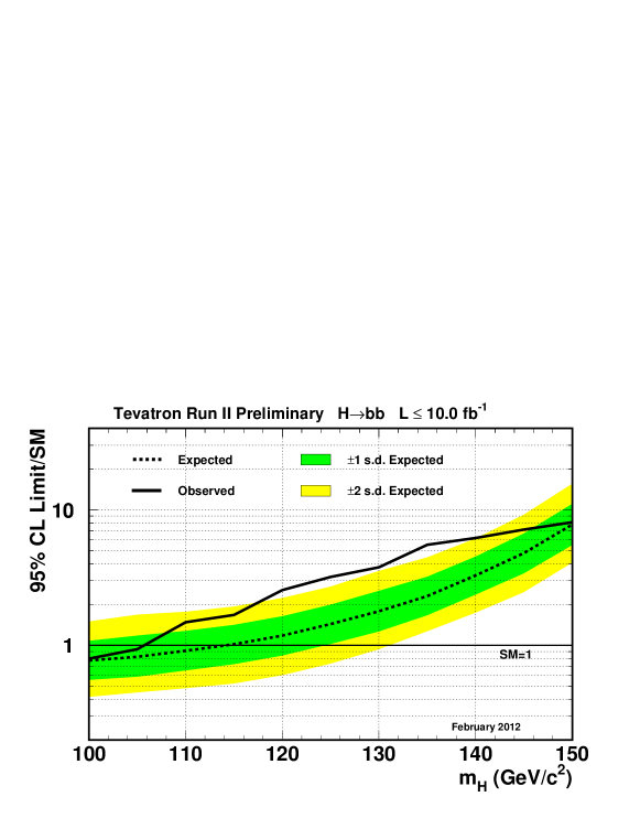
As a final step, we separately combine CDF and D0 searches for , and display the resulting limits on the production cross section times the decay branching ratio normalized to the SM prediction in Figure 21.
In summary, we combine all available CDF and D0 results on SM Higgs boson searches, based on luminosities ranging from 4.3 to 10.0 fb-1. Compared to our previous combination, more data have been added to the existing channels, additional channels have been included, and analyses have been further optimized to gain sensitivity. The results presented here significantly extend the individual limits of each collaboration and those obtained in our previous combination. The sensitivity of our combined search is sufficient to exclude a Higgs boson at high mass and is, in the absence of signal, expected to grow in the future as further improvements are made to our analysis techniques. There is an excess of data events with respect to the background estimation in the mass range GeV/ which causes our limits to not be as stringent as expected. At GeV/, the -value for a background fluctuation to produce this excess is 3.510-3, corresponding to a local significance of 2.7 standard deviations. The global significance for such an excess anywhere in the full mass range is approximately 2.2 standard deviations, after accounting for the look-elsewhere effect.
In addition, we separate the CDF and D0 searches into combinations focusing on the and channels. The largest excess is observed in the channels, corresponding to a local significance of s.d. prior to accounting for the look elsewhere effect of 2, which, when included, yields a global significance of s.d.


| (GeV/ | LLRobs | LLR | LLR | LLR | LLR | LLR | LLR |
|---|---|---|---|---|---|---|---|
| 100 | 4.84 | -6.96 | 16.75 | 11.64 | 6.53 | 1.42 | -3.69 |
| 105 | 3.18 | -6.27 | 15.56 | 10.71 | 5.87 | 1.02 | -3.82 |
| 110 | -2.66 | -5.36 | 14.08 | 9.57 | 5.07 | 0.57 | -3.94 |
| 115 | -5.07 | -4.74 | 12.96 | 8.72 | 4.49 | 0.25 | -3.99 |
| 120 | -8.01 | -3.90 | 11.38 | 7.54 | 3.69 | -0.15 | -3.99 |
| 125 | -4.63 | -3.29 | 10.28 | 6.73 | 3.17 | -0.39 | -3.95 |
| 130 | -6.45 | -3.15 | 9.98 | 6.50 | 3.02 | -0.45 | -3.93 |
| 135 | -6.56 | -3.23 | 10.14 | 6.62 | 3.10 | -0.42 | -3.94 |
| 140 | -2.10 | -3.66 | 10.97 | 7.23 | 3.49 | -0.25 | -3.98 |
| 145 | 2.82 | -4.55 | 12.48 | 8.36 | 4.24 | 0.12 | -4.00 |
| 150 | 5.29 | -5.72 | 14.43 | 9.84 | 5.26 | 0.67 | -3.91 |
| 155 | 6.11 | -7.33 | 16.95 | 11.80 | 6.64 | 1.49 | -3.67 |
| 160 | 14.06 | -13.94 | 25.05 | 18.27 | 11.49 | 4.71 | -2.07 |
| 165 | 16.27 | -15.66 | 26.81 | 19.71 | 12.61 | 5.51 | -1.60 |
| 170 | 6.88 | -10.62 | 21.18 | 15.15 | 9.11 | 3.07 | -2.96 |
| 175 | 3.57 | -7.58 | 17.22 | 12.00 | 6.79 | 1.58 | -3.63 |
| 180 | 2.64 | -5.47 | 13.88 | 9.43 | 4.97 | 0.51 | -3.95 |
| 185 | 0.45 | -3.48 | 10.41 | 6.82 | 3.23 | -0.37 | -3.96 |
| 190 | -1.14 | -2.18 | 7.87 | 4.98 | 2.09 | -0.80 | -3.69 |
| 195 | -4.44 | -1.61 | 6.54 | 4.05 | 1.55 | -0.94 | -3.43 |
| 200 | -3.97 | -1.24 | 5.59 | 3.39 | 1.20 | -0.99 | -3.18 |
| (GeV/) | 1-CL | 1-CL | 1-CL | 1-CL | 1-CL | 1-CL |
|---|---|---|---|---|---|---|
| 100 | 0.980 | 1.000 | 0.999 | 0.989 | 0.933 | 0.726 |
| 105 | 0.958 | 1.000 | 0.998 | 0.985 | 0.914 | 0.680 |
| 110 | 0.707 | 0.999 | 0.996 | 0.976 | 0.881 | 0.612 |
| 115 | 0.463 | 0.999 | 0.994 | 0.966 | 0.850 | 0.559 |
| 120 | 0.148 | 0.998 | 0.988 | 0.945 | 0.796 | 0.479 |
| 125 | 0.347 | 0.996 | 0.982 | 0.925 | 0.748 | 0.415 |
| 130 | 0.174 | 0.995 | 0.979 | 0.918 | 0.734 | 0.400 |
| 135 | 0.175 | 0.996 | 0.981 | 0.922 | 0.742 | 0.409 |
| 140 | 0.634 | 0.997 | 0.986 | 0.938 | 0.779 | 0.454 |
| 145 | 0.934 | 0.999 | 0.992 | 0.961 | 0.838 | 0.541 |
| 150 | 0.979 | 0.999 | 0.996 | 0.978 | 0.892 | 0.639 |
| 155 | 0.988 | 1.000 | 0.999 | 0.990 | 0.939 | 0.745 |
| 160 | 1.000 | 1.000 | 1.000 | 0.999 | 0.993 | 0.943 |
| 165 | 1.000 | 1.000 | 1.000 | 1.000 | 0.996 | 0.961 |
| 170 | 0.994 | 1.000 | 1.000 | 0.998 | 0.979 | 0.877 |
| 175 | 0.971 | 1.000 | 0.999 | 0.991 | 0.943 | 0.758 |
| 180 | 0.941 | 0.999 | 0.995 | 0.974 | 0.881 | 0.619 |
| 185 | 0.813 | 0.996 | 0.982 | 0.928 | 0.760 | 0.436 |
| 190 | 0.582 | 0.985 | 0.952 | 0.852 | 0.619 | 0.288 |
| 195 | 0.125 | 0.971 | 0.918 | 0.787 | 0.530 | 0.219 |
| 200 | 0.103 | 0.952 | 0.882 | 0.727 | 0.459 | 0.173 |
Acknowledgments
We thank the Fermilab staff and the technical staffs of the participating institutions for their vital contributions, and we acknowledge support from the DOE and NSF (USA); CONICET and UBACyT (Argentina); ARC (Australia); CNPq, FAPERJ, FAPESP and FUNDUNESP (Brazil); CRC Program and NSERC (Canada); CAS, CNSF, and NSC (China); Colciencias (Colombia); MSMT and GACR (Czech Republic); Academy of Finland (Finland); CEA and CNRS/IN2P3 (France); BMBF and DFG (Germany); INFN (Italy); DAE and DST (India); SFI (Ireland); Ministry of Education, Culture, Sports, Science and Technology (Japan); KRF, KOSEF and World Class University Program (Korea); CONACyT (Mexico); FOM (The Netherlands); FASI, Rosatom and RFBR (Russia); Slovak R&D Agency (Slovakia); Ministerio de Ciencia e Innovación, and Programa Consolider-Ingenio 2010 (Spain); The Swedish Research Council (Sweden); Swiss National Science Foundation (Switzerland); STFC and the Royal Society (United Kingdom); and the A.P. Sloan Foundation (USA).
References
- (1) CDF Collaboration, “Combination of CDF standard model Higgs boson searches with up to to 9.7 fb-1 of data”,CDF Conference Note 10804 (2012).
- (2) “Combined Upper Limits on Standard Model Higgs Boson Production from the D0 Experiment in up to 9.7 fb-1 of data”, D0 Conference Note 6304 (2012).
- (3) CDF Collaboration, “Measurement of the W Boson Mass using 2.2 fb-1 of CDF II Data”, CDF Conference Note 10775 (2012).
- (4) D0 Collaboration, “Measurement of the W Boson Mass with the D0 Detector”, arXiv:1203.0293v1 [hep-ph] (2012).
- (5) The LEP Electroweak Working Group, ”Status of March 2012”, http://lepewwg.web.cern.ch/LEPEWWG/.
- (6) R. Barate et al. [LEP Working Group for Higgs boson searches], Phys. Lett. B 565, 61 (2003).
- (7) ATLAS Collaboration, “Combined search for the Standard Model Higgs Boson using up to 4.9 fb of pp collision data at = 7 TeV with the ATLAS detector at the LHC”, ATLAS-CONF-2011-163, arXiv:1202.1408 [hep-ex] (2012).
- (8) CMS Collaboration, “Combined results of searches for the standard model Higgs boson in pp collisions at = 7 TeV”, CMS-PAS-HIG-11-032, arXiv:1202.1488 [hep-ex] (2012).
-
(9)
The CDF and D0 Collaborations and the TEVNPH Working Group, “Combined CDF and D0 Upper Limits on Standard Model Higgs Boson Production with up to 8.6 fb-1 of Data,”, FERMILAB-CONF-11-044-E, CDF Note 10606, D0 Note 6226, arXiv:1107.5518v2 [hep-ex] (2011);
The CDF and D0 Collaborations and the TEVNPH Working Group, “Combined CDF and D0 Upper Limits on Standard Model Higgs Boson Production with up to 8.2 fb-1 of Data,”, FERMILAB-CONF-11-044-E, CDF Note 10441, D0 Note 6184, arXiv:1103.3233v1 [hep-ex] (2011);
The CDF and D0 Collaborations and the TEVNPH Working Group, “Combined CDF and D0 Upper Limits on Standard Model Higgs-Boson Production with up to 6.7 fb-1 of Data”, FERMILAB-CONF-10-257-E, CDF Note 10241, D0 Note 6096, arXiv:1007.4587v1 [hep-ex] (2010);
The CDF and D0 Collaborations and the TEVNPH Working Group, “Combined CDF and DZero Upper Limits on Standard Model Higgs-Boson Production with 2.1 to 4.2 fb-1 of Data”, FERMILAB-PUB-09-0557-E, CDF Note 9998, D0 Note 5983, arXiv:0911.3930v1 [hep-ex] (2009).
CDF Collaboration, “Combined Upper Limit on Standard Model Higgs Boson Production for EPS2011”,CDF Conference Note 10609 (2011);
CDF Collaboration, “Search for Production Using 5.9 fb-1”, CDF Conference Note 10432 (2011);
CDF Collaboration, “Combined Upper Limit on Standard Model Higgs Boson Production for ICHEP 2010”,CDF Conference Note 10241 (2010);
CDF Collaboration, “Combined Upper Limit on Standard Model Higgs Boson Production for HCP 2009”, CDF Conference Note 9999 (2009);
CDF Collaboration, “Combined Upper Limit on Standard Model Higgs Boson Production for Summer 2009”, CDF Conference Note 9807 (2009);
D0 Collaboration,“Combined Upper Limits on Standard Model Higgs Boson Production from the D0 Experiment in up to 8.6 fb-1 of data”, D0 Conference Note 6229 (2011);
D0 Collaboration, “Combined Upper Limits on Standard Model Higgs Boson Production in the , and decay modes;
from the D0 Experiment in up to 8.2 fb-1 of data”, D0 Conference Note 6183 (2011);
D0 Collaboration, “Combined Upper Limits on Standard Model Higgs Boson Production from the D0 Experiment in up to 6.7 fb-1 of data”, D0 Conference Note 6094 (2010);
D0 Collaboration,“Combined Upper Limits on Standard Model Higgs Boson Production from the D0 Experiment in 2.1-5.4 fb-1”, D0 Conference Note 6008 (2009);
D0 Collaboration, “Combined upper limits on Standard Model Higgs boson production from the D0 experiment in 0.9-5.0 fb-1”, D0 Conference Note 5984 (2009). -
(10)
CDF Collaboration, “ Inclusive Search for Standard Model Higgs Boson Production in the
WW Decay Channel Using the CDF II Detector”, Phys. Rev. Lett. 104, 061803 (2010);
D0 Collaboration, “ Search for Higgs Boson Production in Dilepton and Missing Energy Final States with 5.4 fb-1 of Collisions at TeV”, Phys. Rev. Lett. 104, 061804 (2010);
The CDF and D0 Collaborations, “Combination of Tevatron Searches for the Standard Model Higgs Boson in the Decay Mode”, Phys. Rev. Lett. 104, 061802 (2010). - (11) W. -Y. Keung and W. J. Marciano, Phys. Rev. D 30, 248 (1984).
- (12) E. W. N. Glover, J. Ohnemus and S. S. D. Willenbrock, Phys. Rev. D 37, 3193 (1988).
- (13) J. F. Gunion, H. E. Haber, G. Kane, and S. Dawson, The Higgs Hunter’s Guide (Addison-Wesley, Boston, 1990).
- (14) M. Dittmar and H. K. Dreiner, Phys. Rev. D 55, 167 (1997).
- (15) S. L. Glashow, D. V. Nanopoulos, and A. Yildiz, Phys. Rev. D 18, 1724 (1978).
- (16) A. Stange, W. J. Marciano and S. Willenbrock, Phys. Rev. D 49, 1354 (1994).
- (17) CDF Collaboration, “Search for standard model Higgs boson production in association with a boson using 9.4 fb-1”, CDF Conference Note 10796 (2012).
- (18) CDF Collaboration, “Search for the standard model Higgs boson in the plus -jets signature in 9.45 fb-1”, CDF Conference Note 10798 (2012).
- (19) CDF Collaboration, “A Search for the standard model Higgs boson in with 9.45 fb-1 of CDF II Data”, CDF Conference Note 10799 (2012).
- (20) CDF Collaboration, “Search for production using 9.7 fb-1”, CDF Conference Note 10785 (2012).
- (21) CDF Collaboration, “Search for with leptons and hadronic taus in the final state using 9.7 fb-1”, CDF Conference Note 10781 (2012).
- (22) CDF Collaboration, “An inclusive search for the Higgs boson in the four lepton final state”, CDF Conference Note 10791 (2012).
- (23) CDF Collaboration, “Search for the standard model Higgs boson in plus jets final state with 8.3 fb-1 of CDF data”, CDF Conference Note 10625 (2011).
- (24) CDF Collaboration, “Search for the standard model Higgs in the and channels”, CDF Conference Note 10500 (2011).
- (25) CDF Collaboration, “A search for the Higgs boson in the all-hadronic channel using 9.45 fb-1”, CDF Conference Note 10792 (2012).
- (26) CDF Collaboration, “Search for a standard model Higgs boson decaying into photons at CDF using 10.0 fb-1 of data”, CDF Conference Note 10737 (2012).
- (27) CDF Collaboration, “Search for the Higgs boson produced in association with top quarks”, CDF Conference Note 10801 (2012).
- (28) CDF Collaboration, “Search for standard model Higgs boson production in association with using no lepton final state”, CDF Conference Note 10582 (2011).
- (29) D0 Collaboration, “Search for Higgs boson in final states with lepton, missing energy and at least two jets in 9.7 fb-1 of Tevatron data,” D0 Conference Note 6309.
- (30) D0 Collaboration, “Search for the standard model Higgs boson in the channel in 9.5 fb-1 of collisions at TeV”, D0 Conference note 6299.
- (31) D0 Collaboration, “A Search for Production in 9.7 fb-1 of Collisions”, D0 Conference Note 6296.
- (32) D0 Collaboration, “Search for the standard model Higgs boson in tau pair final states”, D0 Conference note 6305.
- (33) D0 Collaboration, “Search for associated Higgs boson production with like charged electron muon pairs using 9.7 of collisions at TeV”, D0 Conference Note 6301.
- (34) D0 Collaboration, “ Search for Higgs boson production in dilepton plus missing energy final states with 8.6 - 9.7 fb-1 of collisions at TeV”, D0 Conference Note 6302.
- (35) D0 Collaboration, “A search for the standard model Higgs boson in the Decay Channel”, Phys. Rev. Lett. 106, 171802 (2011).
- (36) D0 Collaboration, “Search for standard model Higgs boson with tri-leptons and missing transverse energy with 9.7 fb-1 of collisions at TeV”, D0 Conference Note 6276.
- (37) D0 Collaboration, “Search for a standard model Higgs boson in the final state with 7.0 fb-1 at TeV”, D0 Conference Note 6286.
- (38) D0 Collaboration, “Search for the Standard Model Higgs boson in + X final states at D0 with 9.7 fb-1 of data”, D0 Conference Note 6295.
- (39) V. M. Abazov et al. [The D0 Collaboration], Nucl. Instrum. Methods A 620, 490 (2010).
- (40) CDF Collaboration, “Higgs optimized -identification tagger at CDF”, CDF Conference Note 10803 (2012).
-
(41)
A. Hoecker, P. Speckmayer, J. Stelzer, J.Therhaag, E. von Toerne, and H. Voss,
“TMVA 4 Toolkit for Multivariate Data Analysis with ROOT User’s Guide” arXiv:physics/0703039a (2007);
C. Cortes and V. Vapnik, “Support vector networks”, Machine Learning 20, 273 (1995);
V. Vapnik, “The Nature of Statistical Learning Theory”, Springer Verlag, New York (1995);
C.J.C. Burges, “A Tutorial on Support Vector Machines for Pattern Recognition”, Data Mining and Knowledge Discovery 2, 1 (1998). - (42) T. Sjöstrand, L. Lonnblad and S. Mrenna, “PYTHIA 6.2: Physics and manual,” arXiv:hep-ph/0108264 (2001).
- (43) M. L. Mangano, M. Moretti, F. Piccinini, R. Pittau and A. D. Polosa, “ALPGEN, a generator for hard multiparton processes in hadronic collisions,” J. High Energy Phys. 0307, 001 (2003).
- (44) S. Frixione and B.R. Webber, J. High Energy Phys. 0206, 029 (2002).
- (45) G. Corcella et al., J. High Energy Phys. 0101, 010 (2001).
-
(46)
A. Pukhov et al.,
“CompHEP: A package for evaluation of Feynman diagrams and integration over
multi-particle phase space. User’s manual for version 33,”
arXiv:hep-ph/9908288 (1999);
E. Boos et al., Nucl. Instrum. Methods A 534, 250 (2004);
E. Boos et al., Phys. Atom. Nucl. 69, 1317 (2006). - (47) J. Campbell and R. K. Ellis, http://mcfm.fnal.gov/.
-
(48)
R. Brun, R. Hagelberg, M. Hansroul, and J. C. Lasalle,
GEANT: Simulation Program for Particle Physics Experiments. User Guide
and Reference Manual, CERN-DD-78-2-REV;
S. Agostinelli et al., Nucl. Instrum. Methods A 506, 250 (2003). - (49) H. L. Lai et al., Phys. Rev D 55, 1280 (1997).
- (50) C. Anastasiou, R. Boughezal and F. Petriello, J. High Energy Phys. 0904, 003 (2009).
- (51) D. de Florian and M. Grazzini, Phys. Lett. B 674, 291 (2009).
- (52) M. Grazzini, private communication (2010).
- (53) The CDF and D0 Collaborations and the Tevatron Electroweak Working Group, arXiv:0903.2503 [hep-ex] (2009).
- (54) R. V. Harlander and W. B. Kilgore, Phys. Rev. Lett. 88, 201801 (2002).
- (55) C. Anastasiou and K. Melnikov, Nucl. Phys. B 646, 220 (2002).
- (56) V. Ravindran, J. Smith, and W. L. van Neerven, Nucl. Phys. B 665, 325 (2003).
- (57) S. Actis, G. Passarino, C. Sturm, and S. Uccirati, Phys. Lett. B 670, 12 (2008).
- (58) U. Aglietti, R. Bonciani, G. Degrassi, A. Vicini, “Two-loop electroweak corrections to Higgs production in proton-proton collisions”, arXiv:hep-ph/0610033v1 (2006).
- (59) S. Catani, D. de Florian, M. Grazzini and P. Nason, “Soft-gluon resummation for Higgs boson production at hadron colliders,” J. High Energy Phys. 0307, 028 (2003).
- (60) A. D. Martin, W. J. Stirling, R. S. Thorne and G. Watt, Eur. Phys. J. C 63, 189 (2009).
-
(61)
http://www.hep.ucl.ac.uk/pdf4lhc/;
S. Alekhin et al., (PDF4LHC Working Group), arXiv:1101.0536v1 [hep-ph] (2011);
M. Botje et al., (PDF4LHC Working Group), arXiv:1101.0538v1 [hep-ph] (2011). - (62) I. W. Stewart, F. J. Tackmann, hys. Rev. D 85, 034011 (2012).
- (63) S. Dittmaier, S. Dittmaier, C. Mariotti, G. Passarino, R. Tanaka, S. Alekhin, J. Alwall and E. A. Bagnaschi et al., arXiv:1201.3084 [hep-ph] (2012).
- (64) C. Anastasiou, G. Dissertori, M. Grazzini, F. Stöckli and B. R. Webber, J. High Energy Phys. 0908, 099 (2009).
- (65) J. M. Campbell, R. K. Ellis, C. Williams, Phys. Rev. D 81, 074023 (2010).
-
(66)
G. Bozzi, S. Catani, D. de Florian, and M. Grazzini, Phys. Lett. B 564, 65 (2003);
G. Bozzi, S. Catani, D. de Florian, and M. Grazzini, Nucl. Phys. B 737, 73 (2006). -
(67)
C. Balazs, J. Huston, I. Puljak, Phys. Rev. D 63 014021 (2001).
C. Balazs and C.-P. Yuan, Phys. Lett. B 478 192-198 (2000).
Qing-Hong Cao and Chuan-Ren Chen, Phys. Rev. D 76 073006 (2007). - (68) J. Baglio and A. Djouadi, J. High Energy Phys. 1010, 064 (2010). We have obtained extended versions of the table of and cross sections for all Higgs boson masses we test, and with more digits of precision, from the authors.
- (69) The Fortran program can be found on Michael Spira’s web page http://people.web.psi.ch/mspira/proglist.html.
- (70) O. Brein, A. Djouadi, and R. Harlander, Phys. Lett. B 579, 149 (2004).
- (71) M. L. Ciccolini, S. Dittmaier, and M. Kramer, Phys. Rev. D 68, 073003 (2003).
- (72) G. Ferrera, M. Grazzini and F. Tramontano, Phys. Rev. Lett. 107, 152003 (2011).
- (73) P. Bolzoni, F. Maltoni, S.-O. Moch, and M. Zaro, Phys. Rev. Lett. 105, 011801 (2010).
-
(74)
M. Ciccolini, A. Denner, and S. Dittmaier,
Phys. Rev. Lett. 99, 161803 (2007);
M. Ciccolini, A. Denner, and S. Dittmaier, Phys. Rev. D 77, 013002 (2008).
We would like to thank the authors of the hawk program for adapting it to the Tevatron. -
(75)
W. Beenaker, S. Dittmaier, M. Krämer, B. Plümper, M. Spira, and P. M. Zerwas,
Phys. Rev. Lett. 87, 201805 (2001);
L. Reina and S. Dawson, Phys. Rev. Lett. 87, 201804 (2001). - (76) S. Dittmaier et al. [ LHC Higgs Cross Section Working Group Collaboration ], arXiv:1101.0593 [hep-ph] (2011).
- (77) A. Djouadi, J. Kalinowski and M. Spira, Comput. Phys. Commun. 108, 56 (1998).
-
(78)
A. Bredenstein, A. Denner, S. Dittmaier, and M. M. Weber,
Phys. Rev. D 74, 013004 (2006);
A. Bredenstein, A. Denner, S. Dittmaier, and M. Weber, J. High Energy Phys. 0702, 080 (2007);
A. Bredenstein, A. Denner, S. Dittmaier, A. Mück, and M. M. Weber, J. High Energy Phys. 0702, 080 (2007) http://omnibus.uni-freiburg.de/~sd565/programs/prophycey4f/prophecy4f.html (2010). - (79) J. Baglio, A. Djouadi, J. High Energy Phys. 1103, 055 (2011).
- (80) A. Denner, S. Heinemeyer, I. Puljak, D. Rebuzzi and M. Spira, Eur. Phys. J. C 71, 1753 (2011).
-
(81)
T. Junk, Nucl. Instrum. Methods A 434, 435 (1999);
A.L. Read, “Modified Frequentist analysis of search results (the method)”, in F. James, L. Lyons and Y. Perrin (eds.), Workshop on Confidence Limits, CERN, Yellow Report 2000-005, available through cdsweb.cern.ch. - (82) W. Fisher, “Systematics and Limit Calculations,” FERMILAB-TM-2386-E.
- (83) V. M. Abazov et al., [D0 Collaboration], Phys. Rev. Lett. 103, 092001 (2009).
- (84) S. Moch and P. Uwer, U. Langenfeld, S. Moch and P. Uwer, Phys. Rev. D 80, 054009 (2009).
-
(85)
M. Cacciari, S. Frixione, M. L. Mangano, P. Nason and G. Ridolfi,
J. High Energy Phys. 0809, 127 (2008).
N. Kidonakis and R. Vogt, Phys. Rev. D 78, 074005 (2008). - (86) N. Kidonakis, Phys. Rev. D 74, 114012 (2006).
- (87) N. Kidonakis, private communication.
- (88) N. Kidonakis, N. Kidonakis, PoS DIS 2010, 196 (2010).
- (89) B. W. Harris, E. Laenen, L. Phaf, Z. Sullivan and S. Weinzierl, Phys. Rev. D 66, 054024 (2002).
- (90) J. Campbell and R. K. Ellis, Phys. Rev. D 65, 113007 (2002).
- (91) E. Gross and O. Vitells, Eur. Phys. J. C 70, 525 (2010).
- (92) Dunn, O.J., “Multiple Comparisons Among Means” Journal of the American Statistical Association, 56, 52-64 (1961).
Appendix A Systematic Uncertainties
CDF: single tight -tag (Tx) channel relative uncertainties (%)
| Contribution | +HF | Mistags | Top | Diboson | Non- | |
| Luminosity () | 3.8 | 0 | 3.8 | 3.8 | 0 | 3.8 |
| Luminosity Monitor | 4.4 | 0 | 4.4 | 4.4 | 0 | 4.4 |
| Lepton ID | 2.0-4.5 | 0 | 2.0-4.5 | 2.0-4.5 | 0 | 2.0-4.5 |
| Jet Energy Scale | 3.2-6.9(S) | 0.9-1.8(S) | 0.8-9.7(S) | 3.6-13.2(S) | 0 | 3.0-5.0(S) |
| Mistag Rate (tight) | 0 | 19 | 0 | 0 | 0 | 0 |
| Mistag Rate (loose) | 0 | 0 | 0 | 0 | 0 | 0 |
| -Tag Efficiency (tight) | 0 | 0 | 3.9 | 3.9 | 0 | 3.9 |
| -Tag Efficiency (loose) | 0 | 0 | 0 | 0 | 0 | 0 |
| Cross Section | 0 | 0 | 10 | 0 | 0 | 0 |
| Diboson Rate | 0 | 0 | 0 | 6.0 | 0 | 0 |
| Signal Cross Section | 0 | 0 | 0 | 0 | 0 | 5 |
| HF Fraction in W+jets | 30 | 0 | 0 | 0 | 0 | 0 |
| ISR+FSR+PDF | 0 | 0 | 0 | 0 | 0 | 3.8-6.8 |
| 3.2-6.9(S) | 0.9-1.8(S) | 0 | 0 | 0 | 0 | |
| QCD Rate | 0 | 0 | 0 | 0 | 40 | 0 |
CDF: single loose -tag (Lx) channel relative uncertainties (%)
| Contribution | +HF | Mistags | Top | Diboson | Non- | |
| Luminosity () | 3.8 | 0 | 3.8 | 3.8 | 0 | 3.8 |
| Luminosity Monitor | 4.4 | 0 | 4.4 | 4.4 | 0 | 4.4 |
| Lepton ID | 2 | 0 | 2 | 2 | 0 | 2 |
| Jet Energy Scale | 2.2-6.0(S) | 0.9-1.8(S) | 1.6-8.6(S) | 4.6-9.6(S) | 0 | 3.1-4.8(S) |
| Mistag Rate (tight) | 0 | 0 | 0 | 0 | 0 | 0 |
| Mistag Rate (loose) | 0 | 10 | 0 | 0 | 0 | 0 |
| -Tag Efficiency (tight) | 0 | 0 | 0 | 0 | 0 | 0 |
| -Tag Efficiency (loose) | 0 | 0 | 3.2 | 3.2 | 0 | 3.2 |
| Cross Section | 0 | 0 | 10 | 0 | 0 | 0 |
| Diboson Rate | 0 | 0 | 0 | 6.0 | 0 | 0 |
| Signal Cross Section | 0 | 0 | 0 | 0 | 0 | 10 |
| HF Fraction in W+jets | 30 | 0 | 0 | 0 | 0 | 0 |
| ISR+FSR+PDF | 0 | 0 | 0 | 0 | 0 | 2.4-4.9 |
| QCD Rate | 2.1-6.0(S) | 0.9-1.8(S) | 0 | 0 | 40 | 0 |
CDF: two tight -tag (TT) channel relative uncertainties (%)
| Contribution | +HF | Mistags | Top | Diboson | Non- | |
| Luminosity () | 3.8 | 0 | 3.8 | 3.8 | 0 | 3.8 |
| Luminosity Monitor | 4.4 | 0 | 4.4 | 4.4 | 0 | 4.4 |
| Lepton ID | 2.0-4.5 | 0 | 2.0-4.5 | 2.0-4.5 | 0 | 2.0-4.5 |
| Jet Energy Scale | 4.0-16.6(S) | 0.9-3.3(S) | 0.9-10.4(S) | 4.7-19.7(S) | 0 | 2.3-13.6(S) |
| Mistag Rate (tight) | 0 | 40 | 0 | 0 | 0 | 0 |
| Mistag Rate (loose) | 0 | 0 | 0 | 0 | 0 | 0 |
| -Tag Efficiency (tight) | 0 | 0 | 7.8 | 7.8 | 0 | 7.8 |
| -Tag Efficiency (loose) | 0 | 0 | 0 | 0 | 0 | 0 |
| Cross Section | 0 | 0 | 10 | 0 | 0 | 0 |
| Diboson Rate | 0 | 0 | 0 | 6.0 | 0 | 0 |
| Signal Cross Section | 0 | 0 | 0 | 0 | 0 | 5 |
| HF Fraction in W+jets | 30 | 0 | 0 | 0 | 0 | 0 |
| ISR+FSR+PDF | 0 | 0 | 0 | 0 | 0 | 6.4-12.6 |
| 4.0-8.8(S) | 0.9-1.8(S) | 0 | 0 | 0 | 0 | |
| QCD Rate | 0 | 0 | 0 | 0 | 40 | 0 |
CDF: one tight and one loose -tag (TL) channel relative uncertainties (%)
| Contribution | +HF | Mistags | Top | Diboson | Non- | |
| Luminosity () | 3.8 | 0 | 3.8 | 3.8 | 0 | 3.8 |
| Luminosity Monitor | 4.4 | 0 | 4.4 | 4.4 | 0 | 4.4 |
| Lepton ID | 2.0-4.5 | 0 | 2.0-4.5 | 2.0-4.5 | 0 | 2.0-4.5 |
| Jet Energy Scale | 3.9-12.4(S) | 0.9-3.3(S) | 1.4-11.5(S) | 5.0-16.0(S) | 2.5-16.1(S) | |
| Mistag Rate (tight) | 0 | 19 | 0 | 0 | 0 | 0 |
| Mistag Rate (loose) | 0 | 10 | 0 | 0 | 0 | 0 |
| -Tag Efficiency (tight) | 0 | 0 | 3.9 | 3.9 | 0 | 3.9 |
| -Tag Efficiency (loose) | 0 | 0 | 3.2 | 3.2 | 0 | 3.2 |
| Cross Section | 0 | 0 | 10 | 0 | 0 | 0 |
| Diboson Rate | 0 | 0 | 0 | 6.0 | 0 | 0 |
| Signal Cross Section | 0 | 0 | 0 | 0 | 0 | 5 |
| HF Fraction in W+jets | 30 | 0 | 0 | 0 | 0 | 0 |
| ISR+FSR+PDF | 0 | 0 | 0 | 0 | 0 | 3.3-10.3 |
| 3.9-7.7(S) | 0.9-1.9(S) | 0 | 0 | 0 | 0 | |
| QCD Rate | 0 | 0 | 0 | 0 | 40 | 0 |
CDF: two loose -tag (LL) channel relative uncertainties (%)
| Contribution | +HF | Mistags | Top | Diboson | Non- | |
| Luminosity () | 3.8 | 0 | 3.8 | 3.8 | 0 | 3.8 |
| Luminosity Monitor | 4.4 | 0 | 4.4 | 4.4 | 0 | 4.4 |
| Lepton ID | 2 | 0 | 2 | 2 | 0 | 2 |
| Jet Energy Scale | 3.6-6.9(S) | 0.9-1.8(S) | 1.7-7.9(S) | 1.2-8.5 | 0 | 2.7-5.4(S) |
| Mistag Rate (tight) | 0 | 0 | 0 | 0 | 0 | 0 |
| Mistag Rate (loose) | 0 | 20 | 0 | 0 | 0 | 0 |
| -Tag Efficiency (tight) | 0 | 0 | 0 | 0 | 0 | 0 |
| -Tag Efficiency (loose) | 0 | 0 | 6.3 | 6.3 | 0 | 6.3 |
| Cross Section | 0 | 0 | 10 | 0 | 0 | 0 |
| Diboson Rate | 0 | 0 | 0 | 6.0 | 0 | 0 |
| Signal Cross Section | 0 | 0 | 0 | 0 | 0 | 10 |
| HF Fraction in W+jets | 30 | 0 | 0 | 0 | 0 | 0 |
| ISR+FSR+PDF | 0 | 0 | 0 | 0 | 0 | 2.0-13.6 |
| QCD Rate | 3.6-6.9(S) | 0.9-1.8(S) | 0 | 0 | 40 | 0 |
Single Tag (TST) channels relative uncertainties (%)
| Contribution | Dibosons | +l.f. | single top | Multijet | |||
| Luminosity | 6.1 | 6.1 | 6.1 | 6.1 | 6.1 | – | 6.1 |
| Electron ID/Trigger eff. (S) | 1–5 | 2–4 | 2–4 | 1–2 | 1–2 | – | 2–3 |
| Muon Trigger eff. (S) | 1 | 1 | 1 | 1 | 1 | – | 1 |
| Muon ID/Reco eff./resol. | 4.1 | 4.1 | 4.1 | 4.1 | 4.1 | – | 4.1 |
| Jet ID/Reco eff. | 2 | 2 | 2 | 2 | 2 | – | 2 |
| Jet Resolution (S) | 1–2 | 2–4 | 2–3 | 2–5 | 1–2 | – | 2 |
| Jet Energy Scale (S) | 4–7 | 1–5 | 2–5 | 2–7 | 1–2 | – | 2–6 |
| Vertex Conf. Jet (S) | 4–6 | 3–4 | 2–3 | 6–10 | 2–4 | – | 3–7 |
| -tag/taggability (S) | 1–3 | 1–4 | 7–10 | 1–6 | 1–2 | – | 2–9 |
| Heavy-Flavor K-factor | – | 20 | – | – | – | – | – |
| Inst.-WH (S) | 1–2 | 2–4 | 1–3 | 1–2 | 1–3 | 15 | 1–2 |
| Inst.-WH | – | 2.4 | 2.4 | – | – | 20 | – |
| Cross Section | 6 | 9 | 6 | 7 | 7 | – | 6.1 |
| Signal Branching Fraction | – | – | – | – | – | – | 1-9 |
| ALPGEN MLM pos/neg(S) | – | – | SH | – | – | – | – |
| ALPGEN Scale (S) | – | SH | SH | – | – | – | – |
| Underlying Event (S) | – | SH | SH | – | – | – | – |
| PDF, reweighting | 2 | 2 | 2 | 2 | 2 | – | 2 |
Loose Double Tag (LDT) channels relative uncertainties (%)
| Contribution | Dibosons | +l.f. | single top | Multijet | |||
| Luminosity | 6.1 | 6.1 | 6.1 | 6.1 | 6.1 | – | 6.1 |
| Electron ID/Trigger eff. (S) | 2–5 | 2–3 | 2–3 | 1–2 | 1–2 | – | 1–2 |
| Muon Trigger eff. (S) | 1 | 1 | 1 | 1 | 1 | – | 1 |
| Muon ID/Reco eff./resol. | 4.1 | 4.1 | 4.1 | 4.1 | 4.1 | – | 4.1 |
| Jet ID/Reco eff. | 2 | 2 | 2 | 2 | 2 | – | 2 |
| Jet Resolution (S) | 1–7 | 2–7 | 2–3 | 2–7 | 2–4 | – | 1–5 |
| Jet Energy Scale (S) | 2–11 | 2–5 | 2–7 | 2–7 | 2–5 | – | 2–8 |
| Vertex Conf. Jet (S) | 2–11 | 2–12 | 2–3 | 4–15 | 2–3 | – | 3–7 |
| -tag/taggability (S) | 2–15 | 2–6 | 6–10 | 2–5 | 2–3 | – | 1–5 |
| Heavy-Flavor K-factor | – | 20 | – | – | – | – | – |
| Inst.-WH (S) | 1–2 | 2–4 | 1–3 | 1–2 | 1–3 | 15 | 1–2 |
| Inst.-WH | – | 2.4 | 2.4 | – | – | 20 | – |
| Cross Section | 6 | 9 | 6 | 7 | 7 | – | 6.1 |
| Signal Branching Fraction | – | – | – | – | – | – | 1-9 |
| ALPGEN MLM pos/neg(S) | – | – | SH | – | – | – | – |
| ALPGEN Scale (S) | – | SH | SH | – | – | – | – |
| Underlying Event (S) | – | SH | SH | – | – | – | – |
| PDF, reweighting | 2 | 2 | 2 | 2 | 2 | – | 2 |
Tight Double Tag (TDT) channels relative uncertainties (%)
| Contribution | Dibosons | +l.f. | single top | Multijet | |||
| Luminosity | 6.1 | 6.1 | 6.1 | 6.1 | 6.1 | – | 6.1 |
| Electron ID/Trigger eff. (S) | 2–5 | 2–3 | 2–3 | 1–2 | 1–2 | – | 1–2 |
| Muon Trigger eff. (S) | 1 | 1 | 1 | 1 | 1 | – | 1 |
| Muon ID/Reco eff./resol. | 4.1 | 4.1 | 4.1 | 4.1 | 4.1 | – | 4.1 |
| Jet ID/Reco eff. | 2 | 2 | 2 | 2 | 2 | – | 2 |
| Jet Resolution (S) | 2–5 | 2–4 | 2–6 | 2–7 | 1–2 | – | 4–6 |
| Jet Energy Scale (S) | 3–8 | 2–5 | 1–8 | 2–9 | 2–4 | – | 2–6 |
| Vertex Conf. Jet (S) | 2–3 | 2–4 | 2–5 | 5–7 | 2–3 | – | 2–4 |
| -tag/taggability (S) | 3–15 | 4–15 | 10–15 | 5–10 | 5–9 | – | 4–12 |
| Heavy-Flavor K-factor | – | 20 | – | – | – | – | – |
| Inst.-WH (S) | 1–2 | 2–4 | 1–3 | 1–2 | 1–3 | 15 | 1–2 |
| Inst.-WH | – | 2.4 | 2.4 | – | – | 20 | – |
| Cross Section | 6 | 9 | 6 | 7 | 7 | – | 6.1 |
| Signal Branching Fraction | – | – | – | – | – | – | 1-9 |
| ALPGEN MLM pos/neg(S) | – | – | SH | – | – | – | – |
| ALPGEN Scale (S) | – | SH | SH | – | – | – | – |
| Underlying Event (S) | – | SH | SH | – | – | – | – |
| PDF, reweighting | 2 | 2 | 2 | 2 | 2 | – | 2 |
Run IIb channel relative uncertainties (%)
| Contribution | +jets | +jets | Top | Dibosons | Multijet | |||
|---|---|---|---|---|---|---|---|---|
| Luminosity | 6.1 | 6.1 | 6.1 | 6.1 | 6.1 | 6.1 | 6.1 | – |
| ID | 2.9 | 2.9 | 2.9 | 2.9 | 2.9 | 2.9 | 2.9 | – |
| trigger | 5.0 | 5.0 | 5.0 | 5.0 | 5.0 | 5.0 | 5.0 | – |
| inclusive trigger relative | 7.0 | 7.0 | 7.0 | 7.0 | 7.0 | 7.0 | 7.0 | – |
| energy correction | 9.8 | 9.8 | 9.8 | 9.8 | 9.8 | 9.8 | 9.8 | – |
| track efficiency | 1.4 | 1.4 | 1.4 | 1.4 | 1.4 | 1.4 | 1.4 | – |
| selection by type | 10,4,5 | 10,4,5 | 10,4,5 | 10,4,5 | 10,4,5 | 10,4,5 | 10,4,5 | – |
| Cross section | 6.2 | 4.9 | 33 | 6.0 | 6.0 | 10.0 | 7.0 | – |
| GGF Signal PDF | – | – | 29 | – | – | – | – | – |
| GGF Reweighting (S) | – | – 5.0 | – | – | – | – | – | – |
| Signal Branching Fraction | 0-7.3 | 0-7.3 | 0-7.3 | – | – | – | – | – |
| Vertex confirmation for jets(S) | 5.0 | 5.0 | 5.0 | 5.0 | 5.0 | 5.0 | 5.0 | – |
| Jet ID(S) | 5 | 5 | 5 | 5 | 5 | 5 | 5 | – |
| Jet Energy Resolution (S) | 5 | 5 | 5 | 5 | 5 | 5 | 5 | – |
| Jet energy Scale (S) | 5 | 5 | 5 | 5 | 5 | 5 | 5 | – |
| Jet pT | 5.5 | 5.5 | 5.5 | 5.5 | 5.5 | 5.5 | 5.5 | – |
| PDF reweighting | 1.6 | 1.6 | 1.6 | 1.6 | 2 | 2 | 2 | – |
| Multijet Normalization | – | – | – | – | – | – | – | 5.3 |
| Multijet Shape | – | – | – | – | – | – | – | 15 |
Run IIb relative uncertainties (%)
| Contribution | +jets | +jets | Top | Dibosons | Multijet | |||
|---|---|---|---|---|---|---|---|---|
| Luminosity | 6.1 | 6.1 | 6.1 | 6.1 | 6.1 | 6.1 | 6.1 | – |
| Electron ID | 4 | 4 | 4 | 4 | 4 | 4 | 4 | – |
| Electron trigger | 2 | 2 | 2 | 2 | 2 | 2 | 2 | – |
| energy correction | 9.8 | 9.8 | 9.8 | 9.8 | 9.8 | 9.8 | 9.8 | – |
| track efficiency | 1.4 | 1.4 | 1.4 | 1.4 | 1.4 | 1.4 | 1.4 | – |
| selection by type | 10,4,5 | 10,4,5 | 10,4,5 | 10,4,5 | 10,4,5 | 10,4,5 | 10,4,5 | – |
| Cross section | 6.1 | 4.9 | 33 | 6.0 | 6.0 | 10.0 | 7.0 | – |
| GGF Signal PDF | – | – | 29 | – | – | – | – | – |
| GGF Reweighting (S) | – | – | 5.0 | – | – | – | – | – |
| Signal Branching Fraction | 0-7.3 | 0-7.3 | 0-7.3 | – | – | – | – | – |
| Vertex confirmation for jets(S) | 5.0 | 5.0 | 5.0 | 5.0 | 5.0 | 5.0 | 5.0 | – |
| Jet ID(S) | 10 | 5 | 5 | 5 | 5 | 5 | 5 | – |
| Jet Energy Resolution (S) | 10 | 10 | 10 | 10 | 10 | 10 | 10 | – |
| Jet energy Scale (S) | 10 | 10 | 10 | 10 | 10 | 10 | 10 | – |
| Jet pT | 5.5 | 5.5 | 5.5 | 5.5 | 5.5 | 5.5 | 5.5 | – |
| PDF reweighting | 1.6 | 1.6 | 1.6 | 1.6 | 2 | 2 | 2 | – |
| Multijet Normalization | – | – | – | – | – | – | – | 4.7 |
| Multijet Shape | – | – | – | – | – | – | – | 15 |
CDF: tight double-tag (SS) channel relative uncertainties (%)
| Contribution | ZH | WH | Multijet | Mistags | Top Pair | S. Top | Diboson | W + HF | Z + HF |
|---|---|---|---|---|---|---|---|---|---|
| Luminosity | 3.8 | 3.8 | 3.8 | 3.8 | 3.8 | 3.8 | 3.8 | ||
| Lumi Monitor | 4.4 | 4.4 | 4.4 | 4.4 | 4.4 | 4.4 | 4.4 | ||
| Tagging SF | 10.4 | 10.4 | 10.4 | 10.4 | 10.4 | 10.4 | 10.4 | ||
| Trigger Eff. (S) | 0.9 | 1.4 | 0.9 | 0.9 | 1.6 | 2.0 | 1.8 | 1.2 | |
| Lepton Veto | 2.0 | 2.0 | 2.0 | 2.0 | 2.0 | 2.0 | 2.0 | ||
| PDF Acceptance | 3.0 | 3.0 | 3.0 | 3.0 | 3.0 | 3.0 | 3.0 | ||
| JES (S) | |||||||||
| ISR/FSR | |||||||||
| Cross-Section | 5 | 5 | 10 | 10 | 6 | 30 | 30 | ||
| Multijet Norm. (shape) | 2.5 | ||||||||
| Mistag (S) | |||||||||
CDF: loose double-tag (SJ) channel relative uncertainties (%)
| Contribution | ZH | WH | Multijet | Mistags | Top Pair | S. Top | Diboson | W + HF | Z + HF |
|---|---|---|---|---|---|---|---|---|---|
| Luminosity | 3.8 | 3.8 | 3.8 | 3.8 | 3.8 | 3.8 | 3.8 | ||
| Lumi Monitor | 4.4 | 4.4 | 4.4 | 4.4 | 4.4 | 4.4 | 4.4 | ||
| Tagging SF | 8.3 | 8.3 | 8.3 | 8.3 | 8.3 | 8.3 | 8.3 | ||
| Trigger Eff. (S) | 1.2 | 1.7 | 1.6 | 0.9 | 1.8 | 2.0 | 2.5 | 1.9 | |
| Lepton Veto | 2.0 | 2.0 | 2.0 | 2.0 | 2.0 | 2.0 | 2.0 | ||
| PDF Acceptance | 3.0 | 3.0 | 3.0 | 3.0 | 3.0 | 3.0 | 3.0 | ||
| JES (S) | |||||||||
| ISR/FSR | |||||||||
| Cross-Section | 5.0 | 5.0 | 10 | 10 | 6 | 30 | 30 | ||
| Multijet Norm. | 1.6 | ||||||||
| Mistag (S) | |||||||||
CDF: single-tag (1S) channel relative uncertainties (%)
| Contribution | ZH | WH | Multijet | Mistags | Top Pair | S. Top | Diboson | W + HF | Z + HF |
|---|---|---|---|---|---|---|---|---|---|
| Luminosity | 3.8 | 3.8 | 3.8 | 3.8 | 3.8 | 3.8 | 3.8 | ||
| Lumi Monitor | 4.4 | 4.4 | 4.4 | 4.4 | 4.4 | 4.4 | 4.4 | ||
| Tagging SF | 5.2 | 5.2 | 5.2 | 5.2 | 5.2 | 5.2 | 5.2 | ||
| Trigger Eff. (S) | 1.2 | 1.7 | 1.6 | 0.9 | 1.8 | 2.0 | 2.5 | 1.9 | |
| Lepton Veto | 2.0 | 2.0 | 2.0 | 2.0 | 2.0 | 2.0 | 2.0 | ||
| PDF Acceptance | 3.0 | 3.0 | 3.0 | 3.0 | 3.0 | 3.0 | 3.0 | ||
| JES (S) | |||||||||
| ISR/FSR | |||||||||
| Cross-Section | 5.0 | 5.0 | 10 | 10 | 6 | 30 | 30 | ||
| Multijet Norm. | 0.7 | ||||||||
| Mistag (S) | |||||||||
medium-tag channel relative uncertainties (%)
| Contribution | Top | +l.f. | Dibosons | Total Bkgd | ||
|---|---|---|---|---|---|---|
| Jet ID/Reco Eff (S) | 2.0 | 2.0 | 2.0 | 2.0 | 1.9 | 2.0 |
| Jet Energy Scale (S) | 1.3 | 1.5 | 2.8 | 1.5 | 1.9 | 0.3 |
| Jet Resolution (S) | 0.5 | 0.4 | 0.5 | 0.8 | 0.5 | 0.9 |
| Vertex Conf. / Taggability (S) | 3.4 | 2.2 | 2.0 | 2.3 | 2.2 | 2.1 |
| b Tagging (S) | 1.5 | 2.6 | 8.0 | 3.6 | 3.7 | 0.6 |
| Lepton Identification | 1.5 | 0.9 | 0.8 | 0.9 | 0.9 | 0.9 |
| Trigger | 2.0 | 2.0 | 2.0 | 2.0 | 1.9 | 2.0 |
| Heavy Flavor Fractions | – | 20.0 | – | – | 8.4 | – |
| Cross Sections | 10.0 | 10.2 | 10.2 | 7.0 | 9.8 | 7.0 |
| Signal Branching Fraction | – | – | – | – | – | 1-9 |
| Luminosity | 6.1 | 6.1 | 6.1 | 6.1 | 5.8 | 6.1 |
| Multijet Normalilzation | – | – | – | – | 1.1 | – |
| ALPGEN MLM (S) | – | – | SH | – | – | – |
| ALPGEN Scale (S) | – | SH | SH | – | – | – |
| Underlying Event (S) | – | SH | SH | – | – | – |
| PDF, reweighting (S) | SH | SH | SH | SH | SH | SH |
| Total uncertainty | 12.8 | 23.8 | 15.1 | 10.8 | 14.2 | 10.0 |
tight-tag channel relative uncertainties (%)
| Contribution | Top | +l.f. | Dibosons | Total Bkgd | ||
|---|---|---|---|---|---|---|
| Jet ID/Reco Eff (S) | 2.0 | 2.0 | 2.0 | 2.0 | 2.0 | 2.0 |
| Jet Energy Scale (S) | 1.0 | 1.6 | 3.9 | 1.6 | 1.6 | 0.5 |
| Jet Resolution (S) | 0.7 | 0.6 | 2.6 | 1.4 | 0.8 | 1.3 |
| Vertex Conf. / Taggability (S) | 3.0 | 1.9 | 2.4 | 2.0 | 2.3 | 1.9 |
| b Tagging (S) | 8.9 | 7.3 | 12.5 | 6.4 | 7.4 | 7.8 |
| Lepton Identification | 1.9 | 0.8 | 0.3 | 0.7 | 1.1 | 0.8 |
| Trigger | 2.0 | 2.0 | 2.0 | 2.0 | 2.0 | 2.0 |
| Heavy Flavor Fractions | – | 20.0 | – | – | 11.0 | – |
| Cross Sections | 10.0 | 10.2 | 10.2 | 7.0 | 10.0 | 7.0 |
| Signal Branching Fraction | – | – | – | – | – | 1-9 |
| Luminosity | 6.1 | 6.1 | 6.1 | 6.1 | 6.1 | 6.1 |
| Multijet Normalilzation | – | – | – | – | 0.2 | – |
| ALPGEN MLM (S) | – | – | SH | – | – | – |
| ALPGEN Scale (S) | – | SH | SH | – | – | – |
| Underlying Event (S) | – | SH | SH | – | – | – |
| PDF, reweighting (S) | SH | SH | SH | SH | SH | SH |
| Total uncertainty | 15.5 | 24.7 | 18.3 | 12.0 | 16.8 | 12.7 |
CDF: tight double tag (TT) channels relative uncertainties (%)
| Contribution | Fakes | Mistags | |||||||
| Luminosity () | 3.8 | 3.8 | 3.8 | 3.8 | 3.8 | 3.8 | 3.8 | ||
| Luminosity Monitor | 4.4 | 4.4 | 4.4 | 4.4 | 4.4 | 4.4 | 4.4 | ||
| Lepton ID | 1 | 1 | 1 | 1 | 1 | 1 | 1 | ||
| Lepton Energy Scale | 1.5 | 1.5 | 1.5 | 1.5 | 1.5 | 1.5 | 1.5 | ||
| Fake | 50 | ||||||||
| Fake | 5 | ||||||||
| Tight Mistag Rate | 40 | ||||||||
| Loose Mistag Rate | |||||||||
| JES [, 2 jet] | |||||||||
| JES [, 3 jet] | |||||||||
| JES [, 2 jet] | |||||||||
| JES [, 3 jet] | |||||||||
| Tight -tag Rate | 7.8 | 7.8 | 7.8 | 7.8 | 7.8 | 7.8 | 7.8 | ||
| Loose -tag Rate | |||||||||
| Cross Section | 10 | ||||||||
| Diboson Cross Section | 6 | 6 | 6 | ||||||
| HF Cross Section | 40 | 40 | |||||||
| Cross Section | 5 | ||||||||
| ISR/FSR | 5.5–7.6 | ||||||||
| Electron Trigger Eff. | 1 | 1 | 1 | 1 | 1 | 1 | 1 | ||
| Muon Trigger Eff. | 5 | 5 | 5 | 5 | 5 | 5 | 5 |
CDF: one tight and one loose tag (TL) channels relative uncertainties (%)
| Contribution | Fakes | Mistags | |||||||
| Luminosity () | 3.8 | 3.8 | 3.8 | 3.8 | 3.8 | 3.8 | 3.8 | ||
| Luminosity Monitor | 4.4 | 4.4 | 4.4 | 4.4 | 4.4 | 4.4 | 4.4 | ||
| Lepton ID | 1 | 1 | 1 | 1 | 1 | 1 | 1 | ||
| Lepton Energy Scale | 1.5 | 1.5 | 1.5 | 1.5 | 1.5 | 1.5 | 1.5 | ||
| Fake | 50 | ||||||||
| Fake | 5 | ||||||||
| Tight Mistag Rate | 19 | ||||||||
| Loose Mistag Rate | 10 | ||||||||
| JES [, 2 jet] | |||||||||
| JES [, 3 jet] | |||||||||
| JES [, 2 jet] | |||||||||
| JES [, 3 jet] | |||||||||
| Tight -tag Rate | 3.9 | 3.9 | 3.9 | 3.9 | 3.9 | 3.9 | 3.9 | ||
| Loose -tag Rate | 3.2 | 3.2 | 3.2 | 3.2 | 3.2 | 3.2 | 3.2 | ||
| Cross Section | 10 | ||||||||
| Diboson Cross Section | 6 | 6 | 6 | ||||||
| HF Cross Section | 40 | 40 | |||||||
| Cross Section | 5 | ||||||||
| ISR/FSR | 3.4–7.0 | ||||||||
| Electron Trigger Eff. | 1 | 1 | 1 | 1 | 1 | 1 | 1 | ||
| Muon Trigger Eff. | 5 | 5 | 5 | 5 | 5 | 5 | 5 |
CDF: single tight tag (TT) channels relative uncertainties (%)
| Contribution | Fakes | Mistags | |||||||
| Luminosity () | 3.8 | 3.8 | 3.8 | 3.8 | 3.8 | 3.8 | 3.8 | ||
| Luminosity Monitor | 4.4 | 4.4 | 4.4 | 4.4 | 4.4 | 4.4 | 4.4 | ||
| Lepton ID | 1 | 1 | 1 | 1 | 1 | 1 | 1 | ||
| Lepton Energy Scale | 1.5 | 1.5 | 1.5 | 1.5 | 1.5 | 1.5 | 1.5 | ||
| Fake | 50 | ||||||||
| Fake | 5 | ||||||||
| Tight Mistag Rate | 19 | ||||||||
| Loose Mistag Rate | |||||||||
| JES [, 2 jet] | |||||||||
| JES [, 3 jet] | |||||||||
| JES [, 2 jet] | |||||||||
| JES [, 3 jet] | |||||||||
| Tight -tag Rate | 3.9 | 3.9 | 3.9 | 3.9 | 3.9 | 3.9 | 3.9 | ||
| Loose -tag Rate | |||||||||
| Cross Section | 10 | ||||||||
| Diboson Cross Section | 6 | 6 | 6 | ||||||
| HF Cross Section | 40 | 40 | |||||||
| Cross Section | 5 | ||||||||
| ISR/FSR | 0.9–12.8 | ||||||||
| Electron Trigger Eff. | 1 | 1 | 1 | 1 | 1 | 1 | 1 | ||
| Muon Trigger Eff. | 5 | 5 | 5 | 5 | 5 | 5 | 5 |
CDF: double loose tag (LL) channels relative uncertainties (%)
| Contribution | Fakes | Mistags | |||||||
| Luminosity () | 3.8 | 3.8 | 3.8 | 3.8 | 3.8 | 3.8 | 3.8 | ||
| Luminosity Monitor | 4.4 | 4.4 | 4.4 | 4.4 | 4.4 | 4.4 | 4.4 | ||
| Lepton ID | 1 | 1 | 1 | 1 | 1 | 1 | 1 | ||
| Lepton Energy Scale | 1.5 | 1.5 | 1.5 | 1.5 | 1.5 | 1.5 | 1.5 | ||
| Fake | 50 | ||||||||
| Fake | 5 | ||||||||
| Tight Mistag Rate | |||||||||
| Loose Mistag Rate | 20 | ||||||||
| JES [, 2 jet] | |||||||||
| JES [, 3 jet] | |||||||||
| JES [, 2 jet] | |||||||||
| JES [, 3 jet] | |||||||||
| Tight -tag Rate | |||||||||
| Loose -tag Rate | 6.3 | 6.3 | 6.3 | 6.3 | 6.3 | 6.3 | 6.3 | ||
| Cross Section | 10 | ||||||||
| Diboson Cross Section | 6 | 6 | 6 | ||||||
| HF Cross Section | 40 | 40 | |||||||
| Cross Section | 5 | ||||||||
| ISR/FSR | 3.1–15.2 | ||||||||
| Electron Trigger Eff. | 1 | 1 | 1 | 1 | 1 | 1 | 1 | ||
| Muon Trigger Eff. | 5 | 5 | 5 | 5 | 5 | 5 | 5 |
Single Tag (ST) channels relative uncertainties (%)
| Contribution | Multijet | +l.f. | Dibosons | Top | |||
| Jet Energy Scale (S) | 4.2 | – | 6.8 | 4.9 | 5.2 | 6.7 | 3.3 |
| Jet Energy Resolution (S) | 1.2 | – | 5.2 | 3.3 | 3.2 | 2.2 | 0.4 |
| Jet ID (S) | 0.3 | – | 0.7 | 0.3 | 0.5 | 0.5 | 0.6 |
| Taggability (S) | 1.5 | – | 1.0 | 1.0 | 1.3 | 1.3 | 0.8 |
| Model (S) | – | – | 2.7 | 1.4 | 1.5 | – | – |
| HF Tagging Efficiency (S) | 0.4 | – | – | 1.1 | 4.0 | – | 1.3 |
| LF Tagging Efficiency (S) | – | – | 73 | – | – | 3.0 | – |
| Multijet Shape (S) | – | 54 | – | – | – | – | – |
| Multijet Normalization | – | 1-70 | – | – | – | – | – |
| +jets Jet Angles (S) | – | – | 1.7 | 2.9 | 3.4 | – | – |
| Alpgen MLM (S) | – | – | 0.3 | – | – | – | – |
| Alpgen Scale (S) | – | – | 0.4 | 0.4 | 0.4 | – | – |
| Underlying Event (S) | – | – | 0.2 | 0.4 | 0.3 | – | – |
| Trigger (S) | 0.4 | – | 0.03 | 0.2 | 0.2 | 0.2 | 0.5 |
| Cross Sections | 6 | – | – | 20 | 20 | 7 | 10 |
| Signal Branching Fraction | 1-9 | – | – | – | – | – | – |
| Normalization | 2.5 | – | 0.3 | 0.3 | 0.3 | 2.5 | 2.5 |
| PDFs | 0.6 | – | 1.0 | 2.4 | 1.1 | 0.7 | 5.9 |
Double Tag (DT) channels relative uncertainties (%)
| Contribution | Multijet | +l.f. | Dibosons | Top | |||
| Jet Energy Scale (S) | 2.6 | – | 7.4 | 6.5 | 5.1 | 5.8 | 1.0 |
| Jet Energy Resolution(S) | 1.0 | – | 4.0 | 4.4 | 4.7 | 0.9 | 0.9 |
| JET ID (S) | 0.8 | – | 0.8 | 0.1 | 0.1 | 0.8 | 0.8 |
| Taggability (S) | 0.9 | – | 0.5 | 1.0 | 0.8 | 0.7 | 0.9 |
| Model (S) | – | – | 1.3 | 1.3 | 2.0 | – | – |
| HF Tagging Efficiency (S) | 5.3 | – | – | 5.7 | 5.9 | – | 4.0 |
| LF Tagging Efficiency (S) | – | – | 47 | – | – | 6.2 | – |
| Multijet Shape (S) | – | 59 | – | – | – | – | – |
| Multijet Normalization | – | 1-70 | – | – | – | – | – |
| +jets Jet Angles (S) | – | – | 1.4 | 3.7 | 3.7 | – | – |
| Alpgen MLM (S) | – | – | 0.2 | – | – | – | – |
| Alpgen Scale (S) | – | – | 0.3 | 0.4 | 0.4 | – | – |
| Underlying Event(S) | – | – | 0.3 | 0.4 | 0.4 | – | – |
| Trigger (S) | 0.4 | – | 0.4 | 0.3 | 0.2 | 0.3 | 0.5 |
| Cross Sections | 6 | – | – | 20 | 20 | 7 | 10 |
| Signal Branching Fraction | 1-9 | – | – | – | – | – | – |
| Normalization | 2.5 | – | 0.3 | 0.3 | 0.3 | 2.5 | 2.5 |
| PDFs | 0.6 | – | 1.0 | 2.4 | 1.1 | 0.7 | 5.9 |
CDF: with no associated jet channel relative uncertainties (%)
| Contribution | DY | +jet | VBF | ||||||||
|---|---|---|---|---|---|---|---|---|---|---|---|
| Cross Section | |||||||||||
| ScaleInclusive | 13.4 | ||||||||||
| Scale1+Jets | |||||||||||
| Scale2+Jets | 0.0 | ||||||||||
| PDF Model | 7.6 | ||||||||||
| Total | 6.0 | 6.0 | 6.0 | 7.0 | 5.0 | 5.0 | 10.0 | ||||
| Acceptance | |||||||||||
| Scale (jets) | 0.3s | ||||||||||
| PDF Model (leptons) | 2.7 | ||||||||||
| PDF Model (jets) | 1.1 | 5.5 | |||||||||
| Higher-order Diagrams | 10.0 | 10.0 | 10.0 | 10.0 | 10.0 | 10.0 | 10.0 | ||||
| Modeling | 19.0 | ||||||||||
| Conversion Modeling | 6.8 | ||||||||||
| Jet Fake Rates | |||||||||||
| (Low S/B) | 15.0 | ||||||||||
| (High S/B) | 24.0 | ||||||||||
| Jet Energy Scale | 3.1 | 6.2 | 3.5 | 28.2 | 18.0 | 3.5 | 5.7 | 9.9 | 5.3 | 12.9 | |
| Lepton ID Efficiencies | 3.8 | 3.8 | 3.8 | 3.8 | 3.8 | 3.8 | 3.8 | 3.8 | 3.8 | ||
| Trigger Efficiencies | 2.0 | 2.0 | 2.0 | 2.0 | 2.0 | 2.0 | 2.0 | 2.0 | 2.0 | ||
| Luminosity | 5.9 | 5.9 | 5.9 | 5.9 | 5.9 | 5.9 | 5.9 | 5.9 | 5.9 |
CDF: with one associated jet channel relative uncertainties (%)
| Contribution | DY | +jet | VBF | ||||||||
|---|---|---|---|---|---|---|---|---|---|---|---|
| Cross Section | |||||||||||
| ScaleInclusive | 0.0 | ||||||||||
| Scale1+Jets | 35.0 | ||||||||||
| Scale2+Jets | |||||||||||
| PDF Model | 17.3 | ||||||||||
| Total | 6.0 | 6.0 | 6.0 | 7.0 | 5.0 | 5.0 | 10.0 | ||||
| Acceptance | |||||||||||
| Scale (jets) | -4.0s | ||||||||||
| PDF Model (leptons) | 3.6 | ||||||||||
| PDF Model (jets) | 4.7 | -6.3 | |||||||||
| Higher-order Diagrams | 10.0 | 10.0 | 10.0 | 10.0 | 10.0 | 10.0 | 10.0 | ||||
| Modeling | 21.0 | ||||||||||
| Conversion Modeling | 6.8 | ||||||||||
| Jet Fake Rates | |||||||||||
| (Low S/B) | 16.0 | ||||||||||
| (High S/B) | 27.0 | ||||||||||
| Jet Energy Scale | -5.8 | -1.1 | -4.8 | -13.1 | -6.5 | -9.5 | -3.8 | -8.5 | -7.8 | -6.8 | |
| Lepton ID Efficiencies | 3.8 | 3.8 | 3.8 | 3.8 | 3.8 | 3.8 | 3.8 | 3.8 | 3.8 | ||
| Trigger Efficiencies | 2.0 | 2.0 | 2.0 | 2.0 | 2.0 | 2.0 | 2.0 | 2.0 | 2.0 | ||
| Luminosity | 5.9 | 5.9 | 5.9 | 5.9 | 5.9 | 5.9 | 5.9 | 5.9 | 5.9 |
CDF: with two or more associated jets channel relative uncertainties (%)
| Contribution | DY | +jet | VBF | ||||||||
|---|---|---|---|---|---|---|---|---|---|---|---|
| Cross Section | |||||||||||
| ScaleInclusive | 0.0 | ||||||||||
| Scale1+Jets | 0.0 | ||||||||||
| Scale2+Jets | 33.0 | ||||||||||
| PDF Model | 29.7 | ||||||||||
| Total | 6.0 | 6.0 | 6.0 | 7.0 | 5.0 | 5.0 | 10.0 | ||||
| Acceptance | |||||||||||
| Scale (jets) | -8.2s | ||||||||||
| PDF Model (leptons) | 4.8 | ||||||||||
| PDF Model (jets) | 4.2 | -12.3 | |||||||||
| Higher-order Diagrams | 10.0 | 10.0 | 10.0 | 10.0 | 10.0 | 10.0 | 10.0 | ||||
| Modeling | 26.0 | ||||||||||
| Conversion Modeling | 6.8 | ||||||||||
| Jet Fake Rates | 19.0 | ||||||||||
| Jet Energy Scale | -20.5 | -13.2 | -13.3 | -1.7 | -32.7 | -22.0 | -15.1 | -4.0 | -2.5 | -3.8 | |
| -tag Veto | 3.6 | ||||||||||
| Lepton ID Efficiencies | 3.8 | 3.8 | 3.8 | 3.8 | 3.8 | 3.8 | 3.8 | 3.8 | 3.8 | ||
| Trigger Efficiencies | 2.0 | 2.0 | 2.0 | 2.0 | 2.0 | 2.0 | 2.0 | 2.0 | 2.0 | ||
| Luminosity | 5.9 | 5.9 | 5.9 | 5.9 | 5.9 | 5.9 | 5.9 | 5.9 | 5.9 |
CDF: low with zero or one associated jets channel relative uncertainties (%)
| Contribution | DY | +jet(s) | VBF | ||||||||
|---|---|---|---|---|---|---|---|---|---|---|---|
| Cross Section | |||||||||||
| ScaleInclusive | 8.1 | ||||||||||
| Scale1+Jets | 0.0 | ||||||||||
| Scale2+Jets | |||||||||||
| PDF Model | 10.5 | ||||||||||
| Total | 6.0 | 6.0 | 6.0 | 7.0 | 5.0 | 5.0 | 5.0 | 10.0 | |||
| Acceptance | |||||||||||
| Scale (jets) | -0.4s | ||||||||||
| PDF Model (leptons) | 1.0 | ||||||||||
| PDF Model (jets) | 1.6 | 2.1 | |||||||||
| Higher-order Diagrams | 10.0 | 10.0 | 10.0 | 10.0 | 10.0 | 10.0 | 10.0 | ||||
| Conversion Modeling | 8.4 | ||||||||||
| Jet Fake Rates | 13.8 | ||||||||||
| Jet Energy Scale | 1.2 | 2.2 | 2.0 | 13.3 | 15.4 | 1.2 | 2.4 | 9.2 | 6.5 | 7.8 | |
| Lepton ID Efficiencies | 3.8 | 3.8 | 3.8 | 3.8 | 3.8 | 3.8 | 3.8 | 3.8 | 3.8 | ||
| Trigger Efficiencies | 2.0 | 2.0 | 2.0 | 2.0 | 2.0 | 2.0 | 2.0 | 2.0 | 2.0 | ||
| Luminosity | 5.9 | 5.9 | 5.9 | 5.9 | 5.9 | 5.9 | 5.9 | 5.9 | 5.9 |
CDF: channel relative uncertainties ( )
| Contribution | +jet | VBF | ||||||||||
| Cross section | 6.0 | 6.0 | 6.0 | 10.0 | 5.0 | 5.0 | 10.3 | 5 | 5 | 10 | ||
| Measured W cross-section | 12 | |||||||||||
| PDF Model | 1.6 | 2.3 | 3.2 | 2.3 | 2.7 | 4.6 | 2.2 | 3.1 | 2.5 | 2.0 | 1.9 | 1.8 |
| Higher order diagrams | 10 | 10 | 10 | 10 | 10 | 10 | 10 | 10 | 10 | 10 | ||
| Conversion modeling | 10 | |||||||||||
| Trigger Efficiency | 0.5 | 0.6 | 0.6 | 0.6 | 0.7 | 0.5 | 0.6 | 0.6 | 0.5 | 0.5 | 0.6 | 0.5 |
| Lepton ID Efficiency | 0.4 | 0.5 | 0.5 | 0.4 | 0.4 | 0.4 | 0.5 | 0.4 | 0.4 | 0.4 | 0.4 | 0.4 |
| ID Efficiency | 1.0 | 1.3 | 1.9 | 1.3 | 2.1 | 0.3 | 2.8 | 1.6 | 1.7 | 2.8 | ||
| Jet into Fake rate | 5.8 | 4.8 | 2.0 | 5.1 | 0.1 | 8.8 | 4.2 | 4.0 | 0.4 | |||
| Lepton into Fake rate | 0.2 | 0.1 | 0.6 | 0.2 | 2.3 | 2.1 | 0.15 | 0.06 | 0.15 | 0.11 | ||
| W+jet scale | 1.6 | |||||||||||
| MC Run dependence | 2.6 | 2.6 | 2.6 | 2.6 | ||||||||
| Luminosity | 3.8 | 3.8 | 3.8 | 3.8 | 3.8 | 3.8 | 3.8 | 3.8 | 3.8 | 3.8 | 3.8 | 3.8 |
| Luminosity Monitor | 4.4 | 4.4 | 4.4 | 4.4 | 4.4 | 4.4 | 4.4 | 4.4 | 4.4 | 4.4 | 4.4 | 4.4 |
CDF: channel relative uncertainties (%)
| Contribution | +jet | VBF | ||||||||||
| Cross section | 6.0 | 6.0 | 6.0 | 10.0 | 5.0 | 5.0 | 10.4 | 5 | 5 | 10 | ||
| Measured W cross-section | 12 | |||||||||||
| PDF Model | 1.5 | 2.1 | 2.9 | 2.1 | 2.5 | 4.3 | 2.0 | 2.9 | 2.6 | 2.2 | 2.0 | 2.2 |
| Higher order diagrams | 10 | 10 | 10 | 10 | 11 | 10 | 10 | 10 | ||||
| Trigger Efficiency | 1.3 | 0.7 | 0.7 | 1.1 | 0.9 | 1.3 | 1.0 | 1.0 | 1.3 | 1.3 | 1.2 | 1.3 |
| Lepton ID Efficiency | 1.1 | 1.4 | 1.4 | 1.1 | 1.2 | 1.1 | 1.4 | 1.3 | 1.0 | 1.0 | 1.0 | 1.0 |
| ID Efficiency | 1.0 | 1.2 | 1.4 | 1.6 | 1.9 | 2.9 | 1.6 | 1.7 | 2.8 | |||
| Jet into Fake rate | 5.8 | 5.0 | 4.4 | 4.4 | 0.2 | 8.8 | 4.5 | 4.2 | 0.4 | |||
| Lepton into Fake rate | 0.06 | 0.05 | 0.09 | 0.04 | 1.9 | 1.2 | 0.04 | 0.02 | 0.02 | 0.04 | ||
| W+jet scale | 1.4 | |||||||||||
| MC Run dependence | 3.0 | 3.0 | 3.0 | 3.0 | ||||||||
| Luminosity | 3.8 | 3.8 | 3.8 | 3.8 | 3.8 | 3.8 | 3.8 | 3.8 | 3.8 | 3.8 | 3.8 | 3.8 |
| Luminosity Monitor | 4.4 | 4.4 | 4.4 | 4.4 | 4.4 | 4.4 | 4.4 | 4.4 | 4.4 | 4.4 | 4.4 | 4.4 |
CDF: channel relative uncertainties (%)
| Contribution | DY | +jet | |||||||
| Cross Section | |||||||||
| Total | 6.0 | 6.0 | 6.0 | 7.0 | 5.0 | 5.0 | 5.0 | ||
| Acceptance | |||||||||
| Scale (jets) | -6.1 | ||||||||
| PDF Model (jets) | 5.7 | ||||||||
| Higher-order Diagrams | 10.0 | 10.0 | 10.0 | 10.0 | 10.0 | 10.0 | 10.0 | ||
| Conversion Modeling | 6.8 | ||||||||
| Jet Fake Rates | 37.7 | ||||||||
| Charge Mismeasurement Rate | 25.0 | 25.0 | |||||||
| Jet Energy Scale | -4.1 | -4.2s | -3.3s | -0.3 | -4.9s | -9.1 | -1.0s | -0.7s | |
| Lepton ID Efficiencies | 3.8 | 3.8 | 3.8 | 3.8 | 3.8 | 3.8 | 3.8 | ||
| Trigger Efficiencies | 2.0 | 2.0 | 2.0 | 2.0 | 2.0 | 2.0 | 2.0 | ||
| Luminosity | 5.9 | 5.9 | 5.9 | 5.9 | 5.9 | 5.9 | 5.9 |
CDF: channel relative uncertainties (%)
| Contribution | Fakes | ||||||
|---|---|---|---|---|---|---|---|
| Cross Section | |||||||
| Total | 6.0 | 6.0 | 10.0 | 7.0 | 5.0 | 5.0 | |
| Acceptance | |||||||
| Higher-order Diagrams | 10.0 | 10.0 | 15.0 | 10.0 | 10.0 | 10.0 | |
| Jet Fake Rates | 22.3 | ||||||
| -Jet Fake Rates | 27.3 | ||||||
| Jet Energy Scale | -3.0 | ||||||
| Lepton ID Efficiencies | 5.0 | 5.0 | 5.0 | 5.0 | 5.0 | 5.0 | |
| Trigger Efficiencies | 2.0 | 2.0 | 2.0 | 2.0 | 2.0 | 2.0 | |
| Luminosity | 5.9 | 5.9 | 5.9 | 5.9 | 5.9 | 5.9 |
CDF: with one associated jet channel relative uncertainties (%)
| Contribution | Fakes | ||||||
|---|---|---|---|---|---|---|---|
| Cross Section | |||||||
| Total | 6.0 | 6.0 | 10.0 | 7.0 | 5.0 | 5.0 | |
| Acceptance | |||||||
| Higher-order Diagrams | 10.0 | 10.0 | 15.0 | 10.0 | 10.0 | 10.0 | |
| Jet Fake Rates | 23.6 | ||||||
| -Jet Fake Rates | 42.0 | ||||||
| Jet Energy Scale | -7.8 | -2.4 | -6.4 | 2.2 | -7.0 | 7.1 | |
| Lepton ID Efficiencies | 5.0 | 5.0 | 5.0 | 5.0 | 5.0 | 5.0 | |
| Trigger Efficiencies | 2.0 | 2.0 | 2.0 | 2.0 | 2.0 | 2.0 | |
| Luminosity | 5.9 | 5.9 | 5.9 | 5.9 | 5.9 | 5.9 |
CDF: with two or more associated jets channel relative uncertainties (%)
| Contribution | Fakes | ||||||
|---|---|---|---|---|---|---|---|
| Cross Section | |||||||
| Total | 6.0 | 6.0 | 10.0 | 7.0 | 5.0 | 5.0 | |
| Acceptance | |||||||
| Higher-order Diagrams | 10.0 | 10.0 | 15.0 | 10.0 | 10.0 | 10.0 | |
| Jet Fake Rates | 18.4 | ||||||
| -Jet Fake Rates | 22.2 | ||||||
| Jet Energy Scale | -18.0 | -15.4 | -16.8 | -2.3 | -20.1 | -5.5 | |
| Lepton ID Efficiencies | 5.0 | 5.0 | 5.0 | 5.0 | 5.0 | 5.0 | |
| Trigger Efficiencies | 2.0 | 2.0 | 2.0 | 2.0 | 2.0 | 2.0 | |
| Luminosity | 5.9 | 5.9 | 5.9 | 5.9 | 5.9 | 5.9 |
channels relative uncertainties (%)
| Contribution | Dibosons | jet | Multijet | |||||
| Luminosity/Normalization | 4 | – | 4 | 4 | 4 | 4 | 4 | 4 |
| Cross Section (Scale/PDF) | 5-7 | – | – | 7 | – | 13-33/8-30 | 5 | 6 |
| n-jet norm | – | 2-15 | – | – | – | – | – | – |
| MET model | – | 5-19 | – | – | – | – | – | – |
| jet norm | – | – | 6-30 | – | – | – | – | – |
| jet ISR/FSR model (s) | – | – | 2-20 | – | – | – | – | – |
| Vertex Confirmation (s) | 1-5 | 1-5 | 1-5 | 5-6 | – | 1-5 | 1-5 | 1-5 |
| Jet identification (s) | 1 | 1 | 1 | 1 | – | 1 | 1 | 1 |
| Jet Energy Scale (s) | 1-5 | 1-5 | 1-5 | 1-4 | – | 1-5 | 1-5 | 1-4 |
| Jet Energy Resolution(s) | 1-4 | 1-4 | 1-4 | 1-4 | – | 1-3 | 1-4 | 1-3 |
| B-tagging (s) | – | – | – | 1-5 | – | – | – | – |
D0: channel relative uncertainties (%)
| Contribution | Diboson | + | Multijet | |||||
|---|---|---|---|---|---|---|---|---|
| Luminosity () | 4.6 | 4.6 | - | 4.6 | - | 4.6 | 4.6 | 4.6 |
| Luminosity Monitor | 4.1 | 4.1 | - | 4.1 | - | 4.1 | 4.1 | 4.1 |
| Trigger | 5.0 | 5.0 | - | 5.0 | - | 5.0 | 5.0 | 5.0 |
| Lepton ID | 3.7 | 3.7 | - | 3.7 | - | 3.7 | 3.7 | 3.7 |
| EM veto | 5.0 | - | - | 5.0 | - | 5.0 | 5.0 | 5.0 |
| Tau Energy Scale (S) | 1.0 | 1.1 | - | 1 | - | 1 | 1 | 1 |
| Jet Energy Scale (S) | 8.0 | 1 | - | 1.8 | - | 2.5 | 2.5 | 2.5 |
| Jet identification (S) | 1 | 1 | - | 7.5 | - | 5.0 | 5.0 | 5.0 |
| Multijet (S) | - | - | - | - | 20-50 | - | - | - |
| Cross Section (scale/PDF) | 7.0 | 4.0 | - | 10 | - | 7/8 | 4.9 | 6.1 |
| Signal Branching Fraction | - | - | - | - | - | 0-7.3 | 0-7.3 | 0-7.3 |
| Modeling | 1.0 | - | 10 | - | - | 3.0 | 3.0 | 3.0 |
like charge electron muon pair channel relative uncertainties (%)
| Contribution | VH | Diboson | Multijet | |||
| Cross section | 6.2 | – | – | 6 | 7 | – |
| Luminosity/Normalization | 4 | – | 4 | 4 | 4 | – |
| Multijet | – | – | – | – | – | 30 |
| Trigger | 2 | 2 | 2 | 2 | 2 | 2 |
| Charge flip | – | 50 | – | 50 | 50 | – |
| W+jets/ | – | – | 10 | – | – | – |
| model | – | – | shape | – | – | – |
| model | – | shape | – | – | – | – |
| W+jets/ ISR/FSR model | – | – | shape | – | – | – |
Trilepton channels relative uncertainties (%)
| Contribution | Dibosons | jet | ||||||
| Luminosity | 6.1 | 6.1 | 6.1 | 6.1 | – | 6.1 | 6.1 | 6.1 |
| Cross Section (Scale/PDF) | 6 | 6 | 6 | 7 | – | 6.2 | 7 | 4.9 |
| 2.5 | 2.5 | 2.5 | 2.5 | – | 2.5 | 2.5 | 2.5 | |
| Electron Identification | 2.5 | 2.5 | 2.5 | 2.5 | – | 2.5 | 2.5 | 2.5 |
| Muon Identification | 4 | 4 | 4 | 4 | – | 4 | 4 | 4 |
| Trigger | 3.5 | 3.5 | 3.5 | 3.5 | – | 3.5 | 3.5 | 3.5 |
| – | – | – | – | 8 | – | – | – | |
| lepton fake rate | – | 30 | 30 | – | – | – | – | – |
| Z- reweighting (s) | – | – | – | – | – | – | – | |
| Electron smearing (s) | – | |||||||
| Muon smearing (s) | – |
+X channels relative uncertainties (%)
| Contribution | Dibosons | Instrumental | |||||
| Luminosity/Normalization | 6 | 6 | 6 | 24 | 6 | 6 | 6 |
| Trigger | 3 | 3 | 3 | – | 3 | 3 | 3 |
| Cross Section (Scale/PDF) | 7 | 6 | 10 | – | 13-33/7.6-30 | 4.9 | 6.2 |
| 2.5 | 2.5 | 2.5 | – | 2.5 | 2.5 | 2.5 | |
| Tau Id per (Type 1/2/3) | 7/3.5/5 | 7/3.5/5 | 7/3.5/5 | – | 7/3.5/5 | 7/3.5/5 | 7/3.5/5 |
| Tau Energy Scale | 1 | 1 | 1 | – | 1 | 1 | 1 |
| Tau Track Match per | 1.4 | 1.4 | 1.4 | – | 1.4 | 1.4 | 1.4 |
| Muon Identification | 2.9 | 2.9 | 2.9 | – | 2.9 | 2.9 | 2.9 |
D0: Run II channel relative uncertainties (%)
| Contribution | Shape | +jets | +jets | Top | Diboson | |||
| Jet energy scale | Y | 0.7 | 3.3 | 1.5 | ||||
| Jet identification | Y | 0.5 | 3.8 | 1.0 | 1.1 | 1.0 | ||
| Jet resolution | Y | 0.5 | ||||||
| Association of jets with PV | Y | 1.2 | 3.2 | 2.9 | 2.4 | |||
| Luminosity | N | n/a | n/a | 6.1 | 6.1 | 6.1 | 6.1 | 6.1 |
| Muon trigger | Y | |||||||
| Electron identification | N | 4.0 | 4.0 | 4.0 | 4.0 | 4.0 | 4.0 | 4.0 |
| Muon identification | N | 4.0 | 4.0 | 4.0 | 4.0 | 4.0 | 4.0 | 4.0 |
| ALPGEN tuning | Y | n/a | n/a | n/a | n/a | n/a | ||
| Cross Section | N | 6 | 6 | 10 | 7 | 10 | 10 | 6 |
| Heavy-flavor fraction | Y | 20 | 20 | n/a | n/a | n/a | n/a | n/a |
| Signal Branching Fraction | N | n/a | n/a | n/a | n/a | 0-7.3 | 0-7.3 | 0-7.3 |
| Y | ||||||||
| Electron channel | Muon channel | |||||||
| Multijet Background | Y | 6.5 | 26 | |||||
CDF: channel relative uncertainties (%)
| Contribution | +jets | VBF | ||||
|---|---|---|---|---|---|---|
| Cross Section : | ||||||
| Scale | 7.0 | |||||
| PDF Model | 7.7 | |||||
| Total | 10.0 | 5.0 | 5.0 | 10.0 | ||
| 3.0 | 3.0 | 3.0 | 3.0 | |||
| Acceptance : | ||||||
| PDF Model | 2.7 | |||||
| Higher-order Diagrams | 2.5 | |||||
| Jet Fake Rates | 50.0 | |||||
| Resolution | s | s | s | s | ||
| Lepton ID Efficiencies | 3.6 | 3.6 | 3.6 | 3.6 | 3.6 | |
| Trigger Efficiencies | 0.4 | 0.5 | 0.5 | 0.5 | 0.5 | |
| Luminosity | 5.9 | 5.9 | 5.9 | 5.9 | 5.9 |
CDF: 4 jets channel relative uncertainties (%)
| 1 tight, 1 loose | 1 tight, loose | 2 tight, 0 loose | 2 tight, loose | tight, loose | ||||||
| Contribution | ||||||||||
| Cross Section | 10 | 10 | 10 | 10 | 10 | |||||
| Cross Section | 10 | 10 | 10 | 10 | 10 | |||||
| Luminosity () | 3.8 | 3.8 | 3.8 | 3.8 | 3.8 | 3.8 | 3.8 | 3.8 | 3.8 | 3.8 |
| Luminosity Monitor | 4.4 | 4.4 | 4.4 | 4.4 | 4.4 | 4.4 | 4.4 | 4.4 | 4.4 | 4.4 |
| -Tag Efficiency | ||||||||||
| Mistag Rate | ||||||||||
| Jet Energy Scale | ||||||||||
| ISR+FSR+PDF | 0.36 | 3.04 | 0.38 | 0.75 | 1.29 | 2.73 | 3.86 | 5.28 | 0.33 | 5.13 |
CDF: 5 jets channel relative uncertainties (%)
| 1 tight, 1 loose | 1 tight, loose | 2 tight, 0 loose | 2 tight, loose | tight, loose | ||||||
| Contribution | ||||||||||
| Cross Section | 10 | 10 | 10 | 10 | 10 | |||||
| Cross Section | 10 | 10 | 10 | 10 | 10 | |||||
| Luminosity () | 3.8 | 3.8 | 3.8 | 3.8 | 3.8 | 3.8 | 3.8 | 3.8 | 3.8 | 3.8 |
| Luminosity Monitor | 4.4 | 4.4 | 4.4 | 4.4 | 4.4 | 4.4 | 4.4 | 4.4 | 4.4 | 4.4 |
| -Tag Efficiency | ||||||||||
| Mistag Rate | ||||||||||
| Jet Energy Scale | ||||||||||
| ISR+FSR+PDF | 3.42 | 2.41 | 11.28 | 0.79 | 5.24 | 2.30 | 3.89 | 3.26 | 3.95 | 2.88 |
CDF: 6 or more jets channel relative uncertainties (%)
| 1 tight, 1 loose | 1 tight, loose | 2 tight, 0 loose | 2 tight, loose | tight, loose | ||||||
| Contribution | ||||||||||
| Cross Section | 10 | 10 | 10 | 10 | 10 | |||||
| Cross Section | 10 | 10 | 10 | 10 | 10 | |||||
| Luminosity () | 3.8 | 3.8 | 3.8 | 3.8 | 3.8 | 3.8 | 3.8 | 3.8 | 3.8 | 3.8 |
| Luminosity Monitor | 4.4 | 4.4 | 4.4 | 4.4 | 4.4 | 4.4 | 4.4 | 4.4 | 4.4 | 4.4 |
| -Tag Efficiency | ||||||||||
| Mistag Rate | ||||||||||
| Jet Energy Scale | ||||||||||
| ISR+FSR+PDF | 13.17 | 0.75 | 17.33 | 2.32 | 12.38 | 1.42 | 20.89 | 1.15 | 14.84 | 0.38 |
CDF: +jets 2-tag channel relative uncertainties (%)
| Contribution | non- | ||
|---|---|---|---|
| Luminosity () | 0 | 3.8 | 3.8 |
| Luminosity Monitor | 0 | 4.4 | 4.4 |
| Jet Energy Scale | 0 | 2 | 11 |
| Trigger Efficiency | 0 | 7 | 7 |
| -Tag Efficiency | 0 | 7 | 7 |
| ISR/FSR | 0 | 2 | 2 |
| 0 | 2 | 2 | |
| Cross Section | 0 | 10 | 0 |
| Cross Section | 0 | 3 | 0 |
| Signal Cross Section | 0 | 0 | 10 |
| Background Modeling | 6 | 0 | 0 |
| Background -tagging | 5 | 0 | 0 |
CDF: +jets 3-tag channel relative uncertainties (%)
| Contribution | non- | ||
|---|---|---|---|
| Luminosity () | 0 | 3.8 | 3.8 |
| Luminosity Monitor | 0 | 4.4 | 4.4 |
| Jet Energy Scale | 0 | 3 | 13 |
| Trigger Efficiency | 0 | 7 | 7 |
| -Tag Efficiency | 0 | 9 | 9 |
| ISR/FSR | 0 | 2 | 2 |
| 0 | 2 | 2 | |
| Cross Section | 0 | 10 | 0 |
| Cross Section | 0 | 5 | 0 |
| Signal Cross Section | 0 | 0 | 10 |
| Background Modeling | 6 | 0 | 0 |
| Background -tagging | 10 | 0 | 0 |
CDF: all jets 2-tag channel relative uncertainties (%)
| Contribution | non- | ||
|---|---|---|---|
| Luminosity () | 0 | 3.8 | 3.8 |
| Luminosity Monitor | 0 | 4.4 | 4.4 |
| Jet Energy Scale | 0 | 11 | 20 |
| Trigger Efficiency | 0 | 7 | 7 |
| -Tag Efficiency | 0 | 7 | 7 |
| ISR/FSR | 0 | 2 | 2 |
| 0 | 2 | 2 | |
| Cross Section | 0 | 10 | 0 |
| Cross Section | 0 | 3 | 0 |
| Signal Cross Section | 0 | 0 | 10 |
| Background Modeling | 9 | 0 | 0 |
| Background -tagging | 5 | 0 | 0 |
CDF: all jets 3-tag channel relative uncertainties (%)
| Contribution | non- | ||
|---|---|---|---|
| Luminosity () | 0 | 3.8 | 3.8 |
| Luminosity Monitor | 0 | 4.4 | 4.4 |
| Jet Energy Scale | 0 | 13 | 22 |
| Trigger Efficiency | 0 | 7 | 7 |
| -Tag Efficiency | 0 | 9 | 9 |
| ISR/FSR | 0 | 2 | 2 |
| 0 | 2 | 2 | |
| Cross Section | 0 | 10 | 0 |
| Cross Section | 0 | 6 | 0 |
| Signal Cross Section | 0 | 0 | 10 |
| Background Modeling | 9 | 0 | 0 |
| Background -tagging | 10 | 0 | 0 |
CDF: channel relative uncertainties (%)
| Contribution | diboson | fakes from SS | W+jets | VBF | |||||||
|---|---|---|---|---|---|---|---|---|---|---|---|
| PDF Uncertainty | - | - | - | - | - | - | - | 1.2 | 0.9 | 2.2 | 4.9 |
| ISR/FSR 1 JET | - | - | - | - | - | - | - | 6.7 | 8.7 | 8.8 | 3.6 |
| ISR/FSR 2 JETS | - | - | - | - | - | - | - | 4.8 | 3.8 | 3.9 | 19.1 |
| JES (S) 1 JET | 9.5 | 8.5 | 8.5 | 14.5 | 0.5 | - | 4.2 | 2.8 | 6.4 | 6.5 | 4.3 |
| JES (S) 2 JETS | 18.9 | 22.3 | 22.3 | 1.3 | 10.7 | - | 15.4 | 5.1 | 3.9 | 3.7 | 14.5 |
| Normalization 1 JET | 2.0 | 5.0 | 5.0 | 10.0 | 6.0 | 1.3 | 14.8 | 5.0 | 5.0 | 10.0 | 23.5 |
| Normalization 2 JETS | 2.0 | 5.0 | 5.0 | 10.0 | 6.0 | 2.5 | 14.8 | 5.0 | 5.0 | 10.0 | 33.0 |
| (e leg) | 0.3 | 0.3 | - | 0.3 | 0.3 | - | - | 0.3 | 0.3 | 0.3 | 0.3 |
| ( leg) | 1.0 | - | 1.0 | 1.0 | 1.0 | - | - | 1.0 | 1.0 | 1.0 | 1.0 |
| ( leg) | 3.0 | 3.0 | 3.0 | 3.0 | 3.0 | - | - | 3.0 | 3.0 | 3.0 | 3.0 |
| 2.4 | 2.4 | - | 2.4 | 2.4 | - | - | 2.4 | 2.4 | 2.4 | 2.4 | |
| 2.6 | - | 2.6 | 2.6 | 2.6 | - | - | 2.6 | 2.6 | 2.6 | 2.6 | |
| 3.0 | 3.0 | 3.0 | 3.0 | 3.0 | - | - | 3.0 | 3.0 | 3.0 | 3.0 | |
| 0.5 | 0.5 | 0.5 | 0.5 | 0.5 | - | - | 0.5 | 0.5 | 0.5 | 0.5 | |
| Luminosity | 5.9 | 5.9 | 5.9 | 5.9 | 5.9 | - | - | 5.9 | 5.9 | 5.9 | 5.9 |
CDF: and channel relative uncertainties (%)
| Contribution | ||||||||||||||
|---|---|---|---|---|---|---|---|---|---|---|---|---|---|---|
| Luminosity | 5.9 | 5.9 | 5.9 | 5.9 | 5.9 | 5.9 | 5.9 | 5.9 | 5.9 | 5.9 | 5.9 | 5.9 | 5.9 | 5.9 |
| Cross Section | 11.7 | 11.7 | 11.7 | 5.0 | 5.0 | 5.0 | 11.7 | 14.1 | 11.7 | 5.0 | 5.0 | 5.0 | 10.0 | 10.0 |
| Z-vertex Cut Efficiency | 0.5 | 0.5 | 0.5 | 0.5 | 0.5 | 0.5 | 0.5 | 0.5 | 0.5 | 0.5 | 0.5 | 0.5 | 0.5 | 0.5 |
| Trigger Efficiency | 1.1 | 1.1 | 1.0 | 1.0 | 1.0 | 1.1 | 1.1 | 1.0 | 0.8 | 1.0 | 1.2 | 1.2 | 1.2 | 1.1 |
| Lepton ID Efficiency | 2.4 | 2.3 | 2.4 | 2.4 | 2.4 | 2.4 | 2.4 | 2.4 | 2.3 | 2.4 | 2.4 | 2.4 | 2.4 | 2.4 |
| Lepton Fake Rate | 10.7 | 8.0 | 26.7 | 26.0 | 26.6 | 15.1 | 27.1 | 22.4 | 22.8 | 28.7 | 2.9 | 2.3 | 15.1 | 13.6 |
| Jet Energy Scale | 1.3 | 1.1 | 0.0 | 3.2 | 5.1 | 0.6 | 6.6 | 0.1 | 2.0 | 0.2 | 0.1 | 0.03 | 0.6 | 0.4 |
| MC stat | 3.7 | 2.9 | 7.6 | 1.5 | 1.7 | 2.2 | 4.1 | 3.1 | 20.0 | 3.1 | 1.5 | 1.4 | 3.8 | 9.4 |
| PDF Model | - | - | - | - | - | - | - | - | - | - | 1.2 | 0.9 | 2.2 | 4.9 |
| ISR/FSR Uncertainties | - | - | - | - | - | - | - | - | - | - | 1.3 | 2.1 | 0.6 | 0.2 |
CDF: and channel relative uncertainties (%)
| Contribution | ||||||||||||||
|---|---|---|---|---|---|---|---|---|---|---|---|---|---|---|
| Luminosity | 5.9 | 5.9 | 5.9 | 5.9 | 5.9 | 5.9 | 5.9 | 5.9 | 5.9 | 5.9 | 5.9 | 5.9 | 5.9 | 5.9 |
| Cross Section | 11.7 | 11.7 | 11.7 | 5.0 | 5.0 | 5.0 | 11.7 | 14.1 | 11.7 | 5.0 | 5.0 | 5.0 | 10.0 | 10.0 |
| Z-vertex Cut Efficiency | 0.5 | 0.5 | 0.5 | 0.5 | 0.5 | 0.5 | 0.5 | 0.5 | 0.5 | 0.5 | 0.5 | 0.5 | 0.5 | 0.5 |
| Trigger Efficiency | 1.4 | 1.4 | 1.1 | 1.1 | 1.3 | 1.1 | 1.4 | 1.1 | 1.0 | 0.7 | 1.3 | 1.3 | 1.2 | 1.2 |
| Lepton ID Efficiency | 2.4 | 2.4 | 2.4 | 2.4 | 2.4 | 2.4 | 2.4 | 2.4 | 2.4 | 2.4 | 2.4 | 2.4 | 2.4 | 2.4 |
| Lepton Fake Rate | 9.0 | 6.5 | 26.6 | 20.8 | 31.4 | 25.2 | 39.4 | 27.8 | 19.3 | 41.9 | 1.6 | 2.5 | 28.5 | 29.2 |
| Jet Energy Scale | 0.0 | 0.3 | 2.2 | 0.0 | 0.8 | 1.5 | 0.5 | 0.8 | 0.0 | 0.0 | 0.2 | 0.1 | 1.7 | 0.0 |
| MC stat | 12.9 | 7.2 | 20.9 | 57.7 | 12.6 | 7.7 | 10.2 | 12.4 | 35.4 | 25.8 | 2.1 | 3.9 | 13.0 | 44.7 |
| PDF Model | - | - | - | - | - | - | - | - | - | - | 1.2 | 0.9 | 2.2 | 4.9 |
| ISR/FSR Uncertainties | - | - | - | - | - | - | - | - | - | - | 0.6 | 0.2 | 0.1 | 0.0 |
CDF: and channel relative uncertainties (%)
| Contribution | ||||||||||||||
|---|---|---|---|---|---|---|---|---|---|---|---|---|---|---|
| Luminosity | 5.9 | 5.9 | 5.9 | 5.9 | 5.9 | 5.9 | 5.9 | 5.9 | 5.9 | 5.9 | 5.9 | 5.9 | 5.9 | 5.9 |
| Cross Section | 11.7 | 11.7 | 11.7 | 5.0 | 5.0 | 5.0 | 11.7 | 14.1 | 11.7 | 5.0 | 5.0 | 5.0 | 10.0 | 10.0 |
| Z-vertex Cut Efficiency | 0.5 | 0.5 | 0.5 | 0.5 | 0.5 | 0.5 | 0.5 | 0.5 | 0.5 | 0.5 | 0.5 | 0.5 | 0.5 | 0.5 |
| Trigger Efficiency | 1.0 | 1.1 | 0.9 | 1.0 | 1.1 | 1.1 | 1.1 | 1.0 | 0.7 | 0.9 | 1.1 | 1.1 | 1.1 | 1.1 |
| Lepton ID Efficiency | 3.3 | 3.3 | 3.3 | 3.3 | 3.3 | 3.3 | 3.3 | 3.3 | 3.3 | 3.3 | 3.3 | 3.3 | 3.3 | 3.3 |
| Lepton Fake Rate | 10.4 | 6.8 | 38.1 | 43.3 | 39.9 | 24.8 | 32.8 | 34.2 | 28.8 | 34.8 | 3.1 | 5.9 | 28.1 | 26.3 |
| Jet Energy Scale | 5.5 | 0.0 | 0.0 | 3.3 | 1.6 | 1.2 | 1.6 | 0.0 | 0.0 | 1.1 | 0.1 | 0.6 | 1.8 | 1.7 |
| MC stat | 12.5 | 8.1 | 16.9 | 18.3 | 12.5 | 4.9 | 12.6 | 14.7 | 70.7 | 8.7 | 2.0 | 3.3 | 9.4 | 18.3 |
| PDF Model | - | - | - | - | - | - | - | - | - | - | 1.2 | 0.9 | 2.2 | 4.9 |
| ISR/FSR Uncertainties | - | - | - | - | - | - | - | - | - | - | 1.2 | 0.5 | 0.4 | 0.04 |
CDF: and channel relative uncertainties (%)
| Contribution | QCD | single-top | diboson | +Jets | VH | VBF | |
| Jet Energy Correction | 9 s | 9 s | 9 s | 9 s | 9 s | 9 s | |
| PDF Modeling | 2 | 2 | |||||
| SecVtx+SecVtx | 7.1 | 7.1 | 7.1 | 7.1 | 7.1 | 7.1 | |
| SecVtx+JetProb | 6.4 | 6.4 | 6.4 | 6.4 | 6.4 | 6.4 | |
| Luminosity | 6 | 6 | 6 | 6 | 6 | 6 | |
| ISR/FSR modeling | 3 s | 3 s | |||||
| Jet Width | s | s | s | s | s | s | |
| Trigger | 3.6 | 3.6 | 3.6 | 3.6 | 3.6 | 3.6 | |
| QCD Interpolation | s | ||||||
| QCD MJJ Tuning | s | ||||||
| QCD NN Tuning | s | ||||||
| cross section | 7 | 7 | 6 | 50 | 5 | 10 |
CDF: channel relative uncertainties (%)
| Channel | CC | CP | C′C | C′P |
| Signal Uncertainties : | ||||
| Luminosity | 6 | 6 | 6 | 6 |
| 14/7/5 | 14/7/5 | 14/7/5 | 14/7/5 | |
| 5 | 2 | 5 | 2 | |
| ISR/FSR | 3 | 4 | 2 | 5 |
| Energy Scale | 0.2 | 0.8 | 0.1 | 0.8 |
| Trigger Efficiency | 1.0 | 1.3 | 1.5 | 6.0 |
| Vertex | 0.07 | 0.07 | 0.07 | 0.07 |
| Conversion ID | – | – | 7 | 7 |
| Detector Material | 0.4 | 3.0 | 0.2 | 3.0 |
| Photon/Electron ID | 1.0 | 2.8 | 1.0 | 2.6 |
| Run Dependence | 3.0 | 2.5 | 1.5 | 2.0 |
| Data/MC Fits | 0.4 | 0.8 | 1.5 | 2.0 |
| Background Uncertainties : | ||||
| Fit Function | 2.8 | 0.9 | 6.1 | 3.3 |
D0: channel relative uncertainties (%)
| Contribution | Background | Signal |
| Luminosity | 6 | 6 |
| Acceptance | – | 2 |
| electron ID efficiency | 2 | – |
| electron track-match inefficiency | 10 | – |
| Photon ID efficiency | 3 | 3 |
| Photon energy scale | 2 | 1 |
| Cross Section | 4 | 10 |
| Background subtraction | 15 | - |
| ONN Shape | 1-5 | - |