Bayesian Parameter Estimation for Latent Markov Random Fields and Social Networks

Abstract

Undirected graphical models are widely used in statistics, physics and machine vision. However Bayesian parameter estimation for undirected models is extremely challenging, since evaluation of the posterior typically involves the calculation of an intractable normalising constant. This problem has received much attention, but very little of this has focussed on the important practical case where the data consists of noisy or incomplete observations of the underlying hidden structure. This paper specifically addresses this problem, comparing two alternative methodologies. In the first of these approaches particle Markov chain Monte Carlo (Andrieu et al., 2010) is used to efficiently explore the parameter space, combined with the exchange algorithm (Murray et al., 2006) for avoiding the calculation of the intractable normalising constant (a proof showing that this combination targets the correct distribution in found in a supplementary appendix online). This approach is compared with approximate Bayesian computation (Pritchard et al., 1999). Applications to estimating the parameters of Ising models and exponential random graphs from noisy data are presented. Each algorithm used in the paper targets an approximation to the true posterior due to the use of MCMC to simulate from the latent graphical model, in lieu of being able to do this exactly in general. The supplementary appendix also describes the nature of the resulting approximation.

Nuffield Department of Clinical Medicine,
University of Oxford,
John Radcliffe Hospital,
Oxford OX3 9DU, UK.
Tel.: +447815763118
richard.g.everitt@gmail.com

Keywords: approximate Bayesian computation, particle Markov chain Monte Carlo, intractable normalising constants, exponential random graphs, graphical models.

1   INTRODUCTION

1.1 Motivation

The subject of this paper is Bayesian inference in models for large numbers of dependant objects, e.g. pixels in an image, people in a social network, or pages on the world wide web. We focus on Markov random fields (MRFs), also known as undirected graphical models (UGMs), which are the models most commonly used for this type of data. Much of the literature (e.g. Murray et al. (2006); Møller et al. (2006)) is devoted to estimating the parameters of these models in the case where the MRF is completely observed, but for real data this is often not the case: in practice observations of the MRF can be noisy or incomplete. As a result, estimation of the parameters of the model presents a significant computational challenge, particularly when using Bayesian estimation in order to account for the missing data in a principled manner.

Let $y\in\mathcal{Y}$ represent noisy or incomplete observations of the hidden variables $x\in\mathcal{X}$. Our aim is to estimate the parameters $\theta\in\Theta$ of a model for this data. Using the Bayesian approach, we describe a joint distribution $p(\theta,x,y)=p(\theta)f(x,y|\theta)$ over $\theta$, $x$ and $y$ and wish to estimate $\theta$ through the posterior distribution:

$$p(\theta|y)\propto\int_{x}p(\theta)f(x,y|\theta)dx.$$ (1)

Our focus is on Monte Carlo methods for simulating from $p(\theta|y)$, and we present two quite general methodologies for achieving this. We apply these methods to two well known types of data: a noisy image (similar to Besag (1986)); and an indirectly observed social network (similar to Caimo and Friel (2011)).

Parameter estimation in problems such as these is often addressed using maximum likelihood (as in Heckerman (1996)), rather than a fully Bayesian approach (aside from the recent work in Møller et al. (2004); Murray et al. (2006); Friel et al. (2009); Koskinen et al. (2010)). In this paper we compare the computational approach taken in these recent papers, which we show is not always appropriate, to alternative computational methods.

In some cases we are also interested in the posterior distribution over the hidden variables $x$ (in the applications described above, this is the case if we wish to infer a denoised Ising model or social network) but this is not our primary focus. A part of the methodology we describe is the use of sequential Monte Carlo (SMC) samplers for simulating from the posterior of $x$, which can be significantly more efficient than using MCMC on these models.

In the remainder of this section we describe MRFs in more detail in section 1.2, and basic methods of inference in these model in section 1.3. Section 1.3 also describes the challenges faced in using these basic inference methods, and this motivates the rest of the paper.

1.2 Models

1.2.1 Markov Random Fields

Throughout the paper, we take $p(\theta)$ to have some simple form that can be both evaluated pointwise and simulated from using standard techniques. The primary purpose of this paper is to discuss computational methods for inference rather than choosing the most appropriate models, therefore we choose a proper prior simply to ensure that the posterior always exists.

We assume that the likelihood $f(x,y|\theta)$ factorises as an MRF, i.e. the joint distribution is completely defined by potential functions over groups of variables known as cliques (Besag, 1974):

$$f(x,y|\theta)=\frac{1}{Z(\theta)}\prod_{j=1}^{M}\Phi_{j}(x,y\in C_{j}|\theta)$$ (2)

where $\Phi_{1:M}$ are potentials on cliques $C_{1:M}$, and the normalising constant

$$Z(\theta)=\int_{x,y}\prod_{j=1}^{M}\Phi_{j}(x,y\in C_{j}|\theta)dxdy$$ (3)

is usually an intractable integral. The methods described in this paper also apply to directed graphical models, which is easier to deal with since the factors of the joint distribution in a directed model are simply conditional distributions that can be normalised independently (Heckerman, 1996), and hence the intractable normalising constant is not present.

1.2.2 Ising Models

The Ising model is a particular MRF that defines a distribution over a random vector $x$ of binary variables each of which can take the value $-1$ or $1$. The distribution is defined by the pairwise interactions between variables as $f(x|\theta_{x})=\exp\left[\theta_{x}\sum_{(i,j)\in\mathbf{N}}x_{i}x_{j}\right]/Z(\theta_{x})$, where $\mathbf{N}$ is a set that defines pairs of nodes that are “neighbours” and, for our purposes, $\theta_{x}>0$. This distribution follows through choosing cliques containing only two nodes, with the potential function $\Phi(x_{i},x_{j}|\theta_{x})=\exp(\theta_{x}x_{i}x_{j})$ for each clique. In this paper we concentrate on the case where $\mathbf{N}$ is chosen so that the variables are arranged in a two-dimensional grid. The study of these models often centres around the phase change that the model exhibits when $\theta_{x}$ passes a critical value: a small $\theta_{x}$ gives a small preference for neighbouring nodes to be the same and results in a high probability that localised groups of variables take on the same value. When $\theta_{x}$ increases above the critical value the joint distribution has the vast majority of its probability mass on the cases where almost every variable takes on the same value.

The Ising model and its generalisation, the Potts model (where the variables can take on more than two states), are frequently used in analysing spatially structured data, especially images. In these applications it is usually the case that the random vector $x$ is observed indirectly through observations $y$. To model the noisy image data used later in the paper, we assume that each $x$ variable has a corresponding $y$ variable representing a noisy observation of the $x$ variable. We then take the joint over the $x$ and $y$ variables to be:

$$f(x,y|\theta)=f(x|\theta_{x})g(y|x,\theta_{y})=\frac{1}{Z(\theta_{x})}\exp\left[\theta_{x}\sum_{(i,j)\in\mathbf{N}}x_{i}x_{j}\right]\frac{1}{Z(\theta_{y})}\exp\left[\theta_{y}\sum_{k=1}^{T}x_{k}y_{k}\right],$$ (4)

where $T$ is the number of pixels in the image, $Z(\theta_{y})=\left(\exp(\theta_{y})+\exp(-\theta_{y})\right)^{T}$ is the normalising constant for all of the potentials on the $(x_{k},y_{k})$ pairs.

1.2.3 Exponential Random Graphs

This section considers the most popular model for social networks: the exponential random graph model (ERGM) or $p^{*}$ model (Wasserman and Pattison, 1996). These models are also used in physics and biology and aim to model data consisting of nodes and edges, which in the social network context represent actors and relationships between these actors. There has been relatively little work on using Bayesian inference for inferring the parameters of ERGMs aside from recent papers by Koskinen et al. (2010); Caimo and Friel (2011).

For an ERGM, the random vector $x$ is defined over the space of all graphs on a set of nodes, with each variable in $x$ representing the presence or absence of a particular edge ($x_{k}$ takes value 1 when edge $k$ is present and 0 when edge $k$ is absent). An ERGM for a graph (which consists of a set of edges over the set of nodes) is then given by:

$$f(x|\theta_{x})=\frac{1}{Z(\theta_{x})}\exp(\theta_{x}^{T}S(x))$$ (5)

where $S(x)$ is a vector of statistics of the graph (e.g. the number of edges, triangles, etc) and $\theta_{x}^{T}$ denotes the transpose of the parameter vector $\theta_{x}$. The normalising constant is intractable due to the extremely large number of possible graphs. ERGMs are simply MRFs defined on the edge space of networks (Frank and Strauss, 1986), with statistics of the network corresponding to particular cliques in the MRF.

We consider the case where the $y$ variables represent noisy observations about the existence of each edge in the network. Analogous to equation (4) we use the model

$$f(x,y|\theta)=f(x|\theta_{x})g(y|x,\theta_{y})=\frac{1}{Z(\theta_{x})}\exp(\theta_{x}^{T}S(x))\frac{1}{Z(\theta_{y})}\exp\left[\theta_{y}\sum_{k=1}^{T}(2x_{k}-1)(2y_{k}-1)\right].$$ (6)

We note that the algorithms described in this paper are also applicable to the alternative missing data scenarios described in Koskinen et al. (2010). In fact, the only specific detail that is required to use the methods in this paper is the factorisation of $x$ as an MRF: the space in which $\theta$ and $y$ lie affects only minor implementation details.

1.3 Inference

1.3.1 Posterior Inference

Recall that the posterior distribution of interest is $p(\theta|y)$. We now consider standard Monte Carlo methods for sampling from this distribution, under MRF models such as those described in the previous section. Throughout the algorithmic sections of this paper we consider the general case where both the observed variables $y$ and unobserved variables $x$ are jointly distributed according to an MRF, with distribution $f(x,y|\theta)$.

The high dimensionality of $x$ leads to the use of Markov chain Monte Carlo (MCMC) for performing the integration in equation (1). Specifically, MCMC is used to simulate from $p(\theta,x|y)$, projecting the obtained points into the marginal space in order to obtain a sample from $p(\theta|y)$. In these circumstances, since it is unclear as to how to propose an efficient move in the joint space of $\theta$ and $x$, the standard approach is to use an MCMC algorithm that updates $\theta$ and $x$ separately through moves on their full conditional distributions (see Murray and Ghahramani (2004); Friel et al. (2009); Koskinen et al. (2010), for example). We shall refer to this method as the “data augmentation” (DA) approach.

Superficially the DA approach may seem to be extremely simple, but for the models described here there are three major difficulties with using this method:

1. Sampling from $p(\theta|x,y)$ is difficult, since this requires the evaluation of the intractable normalising constant in equation (3).

2. Sampling from $p(x|\theta,y)$ can be difficult, since this is usually a distribution with a complicated structure on a high-dimensional space.

3. Using a data augmentation approach may be inefficient, since $x$ and $\theta$ are often highly dependent a posteriori.

These difficulties largely dictate the structure of the remainder of the paper. In section 2 we devise a novel MCMC algorithm for sampling from $p(\theta|y)$ that is designed to minimise the effect of each of these problems, combining the exchange algorithm of Murray et al. (2006) with marginal particle Markov chain Monte Carlo (PMCMC) (Andrieu et al., 2010). In section 3 explore an alternative approach to sampling from $p(\theta|y)$, using approximate Bayesian computation (ABC) (Pritchard et al., 1999) to largely circumvent the difficulties listed above. However, this approach introduces complications of its own. Section 4 applies both approaches to data, with a comparison to the standard DA approach.

Throughout the paper we make use of a single site Gibbs sampler on $p(x|\theta,y)$, and for this reason we devote some space in the remainder of this section to describing this algorithm.

1.3.2 Gibbs Samplers for MRFs

The simplest approach to sampling from $p(x|\theta,y)$ for a MRF model using MCMC is to use single component Metropolis, where the variables are updated one at a time. Variable $k$ is updated using a Metropolis-Hastings step targeting the full conditional $p(x_{k}|x_{\neq k},\theta,y)\propto\prod_{C_{j}\ni x_{k}}\Phi_{j}(x,y\in C_{j}|\theta)$, where the product is over the potentials of all cliques that contain variable $k$. When there are strong dependencies between the variables this results in an inefficient MCMC algorithm. A partial solution might be to update highly correlated variables in blocks: Andrieu et al. (2010) note that to create an efficient algorithm the size of the blocks of variables must be limited, since it becomes more increasingly difficult to design good proposals for a block as the size of the block grows. The inefficiency of Gibbs samplers for Ising models is well known (e.g. Higdon (1998)) and a similar observation is made in the literature on ERGMs (Snijders, 2002). Similar approaches, with the same drawbacks, are commonly used for sampling from $p(x|\theta)$, which is encountered both in the exchange and ABC algorithms later in the paper. The inefficiency of these approaches motivates the use of SMC samplers, where we observe a significant improvement over the Gibbs sampler.

2   EXCHANGE MARGINAL PMCMC

This section describes the design of an MCMC algorithm for simulating from $p(\theta|y)$ that addresses the problems listed in section 1.3.1. We begin in section 2.1 by describing methods for sampling from $p(\theta|x,y)$ that avoid the evaluation of the intractable term $Z(\theta)$ in equation (3). Our favoured approach is the exchange algorithm of Murray et al. (2006): an algorithm that requires exact simulation from $f(x,y|\theta)$ which is not generally possible in the models we consider. We study the effect of replacing exact simulation with the use of MCMC.

The remainder of the section focuses on the use of marginal PMCMC to sample efficiently in cases where $\theta$ and $x$ are highly dependant a posteriori. In section 2.2 we introduce PMCMC and describe how to apply it to MRFs, using the exchange algorithm to avoid the intractable normalising constant. The key component of a PMCMC algorithm is an efficient SMC sampler for simulating from $p(x|\theta,y)$ and we describe candidate approaches in section 2.3.

2.1 Intractable Normalising Constant

Consider the use of a Metropolis-Hastings (MH) update on the full conditional $p(\theta|x,y)\propto p(\theta)f(x,y|\theta)$. Let $\gamma(x,y|\theta)=\prod_{j=1}^{M}\Phi_{j}(x,y\in C_{j}|\theta)$ so that $f(x,y|\theta)=\frac{1}{Z(\theta)}\gamma(x,y|\theta)$. Using a proposal $q(\theta^{*}|\theta)$, we obtain the acceptance probability:

$$1\wedge\frac{p(\theta^{*})\gamma(x,y|\theta^{*})q(\theta|\theta^{*})}{p(\theta)\gamma(x,y|\theta)q(\theta^{*}|\theta)}\frac{Z(\theta)}{Z(\theta^{*})},$$ (7)

which cannot be calculated due to the presence of $Z(.)$, leading such models to be known as doubly intractable (Murray et al., 2006). A similar problem is encountered when using maximum likelihood, or any other method that need to evaluate the likelihood. There are several different classes of approaches for avoiding this: pseudo-likelihood (Besag, 1975); variational approximations (Murray and Ghahramani, 2004); Monte Carlo approximations (Geyer and Thompson, 1992; Green and Richardson, 2002; Atchadé et al., 2008); auxiliary variable approaches (Møller et al., 2006; Murray et al., 2006); and ABC (Grelaud et al., 2009). Each of the methods results in targeting an approximation to $p(\theta|x,y)$, unless exact simulation from $f(x,y|\theta)$ is available. We focus on auxiliary variable methods and ABC due to their ease of implementation and because we find that using an MCMC algorithm in place of exact simulation from $f(x|\theta)$ has little practical effect on the examples we consider.

2.1.1 The Single Auxiliary Variable Method

The first MCMC method that targets the true posterior in the presence of the intractable normalising constant was the single auxiliary variable method (SAVM), which originated in Møller et al. (2004) and Møller et al. (2006). Here we present an alternative justification of SAVM to that in the original paper (given in Andrieu et al. (2010)), based on the principle that it is possible to design an MCMC algorithm for simulating from some target $\pi(\text{$\theta$)}$ when only unbiased positive estimates $\widehat{\pi}(\theta)$ of an unnormalised version of $\pi$ are available. Specifically, a standard Metropolis-Hastings algorithm that targets $\widehat{\pi}$, with proposal $q(\theta^{*}|\theta)$ and acceptance probability

$$1\wedge\frac{\widehat{\pi}(\theta^{*})}{\widehat{\pi}(\theta)}\frac{q(\theta|\theta^{*})}{q(\theta^{*}|\theta)},$$ (8)

has a stationary distribution of $\pi(\text{$\theta$)}$. Recall now the MH algorithm targeting $p(\theta|x,y)$ with acceptance probability given in equation (7): equation (8) implies that a Metropolis-Hastings algorithm targeting an unbiased estimate $\widehat{p}(\theta|x,y):=p(\theta)\gamma(x,y|\theta)\widehat{1/Z}(\theta)$ of $p(\theta|x,y)$, where $\widehat{1/Z}(\theta)$ is an unbiased estimate of $1/Z(\theta)$, will have a stationary distribution of $p(\theta|x,y)$.

SAVM targets a joint distribution $\pi(\theta,u|x,y)\propto q_{\mbox{u}}(u|\theta,x,y)p(\theta)\gamma(x,y|\theta)/Z(\theta)$, of which $p(\theta|x,y)$ is a marginal, constructed through the introduction of an auxiliary variable $u$, where $q_{\mbox{u}}(.|\theta,x,y)$ is an arbitrary distribution and $u=(u_{x},u_{y})\in X\times Y$. This target is then simulated using a Metropolis-Hastings algorithm on the $(\theta,u)$ space, with proposal $\theta^{*}\sim q(.|\theta)$ and $u^{*}\sim f(.|\theta^{*})$ (the simulation of $u^{*}$ being performed using exact sampling). The acceptance probability for this move is given by:

$$1\wedge\frac{p(\theta^{*})\gamma(x,y|\theta^{*})q(\theta|\theta^{*})q_{u}(u^{*}|\theta^{*},x,y)\gamma(u|\theta)}{p(\theta)\gamma(x,y|\theta)q(\theta^{*}|\theta)q_{u}(u|\theta,x,y)\gamma(u^{*}|\theta^{*})}.$$ (9)

Comparing equations (7) and (9) we see that essentially SAVM is using single point importance sampling (IS) estimates of $\widehat{1/Z}(\theta)$ and $\widehat{1/Z}(\theta^{*})$, where $\widehat{1/Z}(\theta)=q_{u}(u|\theta,x,y)/\gamma(u|\theta)$ and $\widehat{1/Z}(\theta^{*})=q_{u}(u^{*}|\theta^{*},x,y)/\gamma(u^{*}|\theta^{*})$. Linking this to the argument based on equation (8) gives us an alternative justification of the algorithm which suggests the following generalisation: any algorithm that finds an unbiased estimate of $\widehat{1/Z}(\theta)$ may be used in place of IS. For example, an SMC sampler with $\pi_{1}=f(.|\theta)$ and $\pi_{T}=q_{u}(u|\theta,x,y)$ will provide such an estimate whose efficiency is less dependent on the choice of $q_{u}$ than is the IS estimate. Note that SMC samplers play an important role later in the paper, and we refer the reader unfamiliar with the method to Del Moral et al. (2006) for further details.

2.1.2 The Exchange Algorithm

In Murray et al. (2006), the exchange algorithm is initially motivated by the observation that in SAVM the ratio $Z(\theta)/Z(\theta^{*})$ is estimated indirectly, using the ratio of $\widehat{1/Z}(\theta^{*})$ and $\widehat{1/Z}(\theta)$. Murray et al. (2006) suggests that estimating $Z(\theta)/Z(\theta^{*})$ directly may lead to an improved algorithm. The resulting algorithm is actually most clearly formulated (for our purposes) in an alternative fashion. Consider the target distribution $\pi(\theta,\theta^{*},u|x,y)=f(x,y|\theta)p(\theta)q(\theta^{*}|\theta)f(u|\theta^{*})/p(x,y)$ of which $\pi(\theta|x,y)$ is a marginal, where $u=(u_{x},u_{y})\in\mathcal{X}\times\mathcal{Y}$. At iteration $i$, the exchange algorithm iterates the following two operations (given input $(\theta(i-1),\theta^{*}(i-1),u(i-1))=(\theta,\theta^{*},u)$ from the previous iteration), giving an MCMC algorithm that targets $\pi(\theta,\theta^{*},u|x,y)$:

1. Draw $\theta^{*}\sim q(.|\theta(i-1))$ and $u\sim f(.|\theta^{*})$.

2. Let $(\theta(i),\theta^{*}(i),u(i))=(\theta^{*},\theta(i-1),u)$ with probability:

   $$1\wedge\frac{p(\theta^{*})\gamma(x,y|\theta^{*})q(\theta|\theta^{*})\gamma(u|\theta)}{p(\theta)\gamma(x,y|\theta)q(\theta^{*}|\theta)\gamma(u|\theta^{*})}\frac{Z(\theta)Z(\theta^{*})}{Z(\theta^{*})Z(\theta)}=1\wedge\frac{p(\theta^{*})\gamma(x,y|\theta^{*})q(\theta|\theta^{*})\gamma(u|\theta)}{p(\theta)\gamma(x,y|\theta)q(\theta^{*}|\theta)\gamma(u|\theta^{*})},$$ (10)

   otherwise set $(\theta(i),\theta^{*}(i),u(i))=(\theta(i-1),\theta^{*}(i-1),u)$.

This deterministic move simply proposes a swap of $\theta$ and $\theta^{*}$, hence the name “exchange algorithm”. The proof that this is the appropriate acceptance probability for this move is given in Tierney (1998), where it is established that the acceptance probability for a deterministic move $\theta\rightarrow T(\theta)$ on a target $\pi$ is $1\wedge\pi(T(\theta))/\pi(\theta)$. If we now compare equation (7) with equation (11) we see that $\gamma(u|\theta)/\gamma(u|\theta^{*})$ can be thought of as an IS estimate of $Z(\theta)/Z(\theta^{*})$, so that the exchange method can be interpreted as using an estimate of the acceptance probability. However, we note that in this case we only have proof that this estimate in particular results in an algorithm that targets the correct distribution - alternative estimates that give a better estimate of this ratio may not be appropriate (although the similar approach of Koskinen (2008) is also shown to have the correct target). The exchange method exhibits superior performance to SAVM in Murray et al. (2006), and it is also easier to implement - in SAVM there are more algorithmic choices to make and these can severely affect the performance of the algorithm. For these reasons we focus on the exchange algorithm for the remainder of the paper, although we note that if the free choices in SAVM are well made (as in Møller et al. (2004)), it may outperform the exchange method.

Although the exchange algorithm targets the true posterior, it is less efficient than a standard MH algorithm would be if the true target were available. This inefficiency is accentuated if the proposed $u\sim f(.|\theta^{*})$ has only a small probability of being generated under $\theta$. Murray et al. (2006) describes an extended exchange method to improve this inefficiency whilst maintaining the exactness of the algorithm, using annealed IS (Neal, 2001) as a substitute for the importance estimate $\gamma(u|\theta)/\gamma(u|\theta^{*})$. In the applications described in section 4 we found the use of this extended method to be essential in obtaining a reasonable performance for the methods described in the paper. The central idea of the extended method is to move the proposed $u\sim f(.|\theta^{*})$ through a sequence of transitions so that it has a larger probability of being generated under $\theta$ (a similar idea may be used to improve SAVM in a similar way). This is done by introducing a sequence of $K$ target distributions $f_{k}(.|\theta,\theta^{*})\propto\gamma_{k}(.|\theta,\theta^{*})=\gamma(.|\theta^{*})^{\beta_{k}}\gamma(.|\theta)^{1-\beta_{k}}$ where, for example, $\beta_{k}=(K-k+1)/(K+1)$ so that the sequence of targets provides a “route” from $f(.|\theta^{*})$ to $f(.|\theta)$. The extended exchange algorithm moves the initial point $u\sim f(.|\theta^{*})$ via a sequence of transitions $R_{k}(u^{\prime}|u,\theta,\theta^{*})$ that satisfy detailed balance with $f_{k}(u^{\prime}|\theta,\theta^{*})$, and changes the acceptance probability accordingly:

1. Draw $\theta^{*}\sim q(.|\theta(i-1))$ and $u_{0}\sim f(.|\theta^{*})$.

2. Apply the sequence of transitions: $u_{1}\sim R_{1}(u_{1}|u_{0},\theta,\theta^{*})$, $u_{2}\sim R_{2}(u_{2}|u_{1},\theta,\theta^{*})$, … , $u_{K}\sim R_{K}(u_{K}|u_{K-1},\theta,\theta^{*})$.

3. Let $(\theta(i),\theta^{*}(i),u(i))=(\theta^{*},\theta(i-1),u_{K})$ with probability:

   $$1\wedge\frac{p(\theta^{*})\gamma(x,y|\theta^{*})q(\theta|\theta^{*})}{p(\theta)\gamma(x,y|\theta)q(\theta^{*}|\theta)}\prod_{k=0}^{K}\frac{\gamma_{k+1}(u_{k}|\theta,\theta^{*})}{\gamma_{k}(u_{k}|\theta,\theta^{*})},$$ (11)

   otherwise set $(\theta(i),\theta^{*}(i),u(i))=(\theta(i-1),\theta^{*}(i-1),u_{K})$.

For our applications we have the factorisation $f(x,y|\theta)=f(x|\theta)g(y|x,\theta)$, where $f(x|\theta)=\gamma(x|\theta)/Z(\theta)$ has an intractable normalising constant and $g(y|x,\theta)$ is normalised. In this situation the exchange algorithm is simplified slightly since $u_{y}$ does not need to be simulated.

2.1.3 The Exchange Algorithm Without Exact Simulation

In step 1 of the exchange algorithm, on sampling $u$, exact simulation from the likelihood is required. However, aside from a few special cases (one of which is the Ising model, which can be sampled exactly using “coupling from the past” (Propp and Wilson, 1996)) this is not generally possible for MRFs. Caimo and Friel (2011) choose to approximate the exact simulation by sampling $u$ from $f(.|\theta^{*})$ using an MCMC run that is “long enough” to get a point that can be treated as if it were simulated exactly from $f(.|\theta^{*})$. We refer to this approach as the approximate exchange algorithm, and use $M$ to denote the number of iterations of the MCMC algorithm used to simulate approximately from the likelihood. Caimo and Friel (2011) suggest that 500 iterations is a long enough run for models similar to those studied in this paper, a conclusion supported by own study which suggests that as few as 50 or 100 iterations are usually sufficient. In appendix B in the supplemental materials we give theoretical justification for the validity of this approach, proving that (using a similar method to a proof in Andrieu and Roberts (2009)) when the MCMC kernel for the exact exchange algorithm is uniformly ergodic, the invariant distribution (when it exists) of the corresponding approximate exchange algorithm becomes closer to the “true” target (that of the exact exchange algorithm) with increasing $M$. We also characterise the rate of convergence of the approximate kernel. The same proof justifies the use of an MCMC kernel as a substitute for simulating exactly from the likelihood within SAVM.

2.2 Marginal PMCMC

2.2.1 The Pseudo-Marginal Approach

Our primary concern in this section is problem 3 in section 1.3.1: that the data augmentation approach to obtaining a sample from $p(\theta|y)$ is inefficient when $\theta$ and $x$ are highly dependant a posteriori. The phase change in Ising models means that this dependence is particularly clear in these models, but other MRFs (including ERGMs (Snijders, 2002)) also have this property. Beaumont (2003) and Andrieu and Roberts (2009) describe an alternative approach to sampling from $p(\theta|y)$ that is designed to avoid the problems caused by this dependence: approximating the “ideal” algorithm that uses an MH update by replacing $p(\theta|y)$ with unbiased estimates of the form $\widetilde{p}(\theta|y)$ to $p(\theta|y)$. The argument described in section 2.1.1 tells us that such updates actually provide us with points from the desired target $p(\theta|y)$. Such an approach is referred to as a pseudo-marginal approach. The efficiency of the MCMC chain based on these updates depends on the variance of the estimator $\widetilde{p}(\theta|y)$.

The simplest useful estimator $\widetilde{p}(\theta|y)$ is an IS approximation $\widetilde{p}^{N}(\theta|y)=\frac{1}{N}\sum_{k=1}^{N}p(\theta,x^{(k)}|y)/q(x^{(k)}|\theta)$, where $x^{(k)}\sim q(.|\theta)$. However, for the applications about which we are interested, where $x$ is high-dimensional, it is difficult to define a proposal distribution $q$ that results in an estimator with a small variance. The optimal proposal is $p(x|\theta,y)$ (see (Geyer, 2011), for example): which we cannot sample from directly. The remainder of this section is devoted to using SMC samplers for this task. The framework of PMCMC in Andrieu et al. (2010) then tells us, via the pseudo-marginal approach, how to use SMC samplers to more efficiently obtain samples from $p(\theta|y)$. In section 2.2.2 we describe the marginal PMCMC framework, then in section 2.2.3 we describe the use of marginal PMCMC on MRFs.

2.2.2 Marginal PMCMC

As in Andrieu et al. (2010), in this section we make the assumption (relaxed in the following section) that the normalising constant $Z$ of $f(x,y|\theta)$ is independent of $\theta$ so that the joint posterior is given by: $p(\theta,x|y)=p(\theta)\gamma(x,y|\theta)/Zp(y)$. We describe the marginal PMCMC algorithm briefly here - for a thorough description see Andrieu et al. (2010). The algorithm is an MCMC sampler that targets $p(\theta,x|y)$, operating on the factorisation $p(\theta|y)p(x|\theta,y)$. The intuition behind the approach is in devising a move on the joint $(\theta,x)$ space: in terms of moving around the $\theta$ space it would be most efficient if the proposal could take the form $q(\theta^{*}|\theta)p(x^{*}|\theta^{*},y)$, so that $x^{*}$ is “perfectly adapted” to the proposed $\theta^{*}$. The approach is to devise an algorithm that approximates this idealised situation, using an SMC sampler as a statistically efficient method for simulating from an approximation $\widehat{p}(x^{*}|\theta^{*},y)$ to $p(x^{*}|\theta^{*},y)$. The point from $\widehat{p}(x^{*}|\theta^{*},y)$ is then used as a proposed point in a Metropolis-Hastings algorithm that targets $p(x^{*}|\theta^{*},y)$. Andrieu et al. (2010) derive the acceptance probability that should be used by explicitly writing down the target and proposal distributions involved. The resulting algorithm in the case we describe here proceeds as follows.

At iteration $i$, beginning with the point $(\theta(i-1),x(i-1))$ and the estimate $\widehat{\phi}(i-1)$ outputted from iteration $i-1$:

1. Simulate $\theta^{*}\sim q(.|\theta(i-1))$, where $q$ is some proposal distribution.

2. Run an SMC sampler on the $x$ space, with the final (unnormalised) distribution as $\pi_{T}(x)=\gamma(x,y|\theta^{*})$. This gives a particle approximation $\widehat{p}(x|\theta^{*},y)$ to $p(x|\theta^{*},y)$ and an estimate $\widehat{\phi}(\theta^{*},y)$ of its normalising constant, $\phi(\theta^{*},y)=Zp(y|\theta^{*})$.

3. Sample a single point $x^{*}$ from $\widehat{p}(.|\theta^{*},y)$.

4. Set $(\theta(i),x(i),\widehat{\phi}(i))=(\theta^{*},x^{*},\widehat{\phi}(\theta^{*},y))$ with probability

   $$1\wedge\frac{p(\theta^{*})\widehat{\phi}(\theta^{*},y)}{p(\theta)\widehat{\phi}(i-1)}\frac{q(\theta(i-1)|\theta^{*})}{q(\theta^{*}|\theta(i-1))},$$ (12)

   otherwise set $(\theta(i),x(i),\widehat{\phi}(i))=(\theta(i-1),x(i-1),\widehat{\phi}(i-1))$.

Here note the interpretation of the algorithm as a Metropolis-Hastings algorithm targeting an unbiased approximation to $p(\theta|y)\propto p(\theta)\phi(\theta,y)=p(\theta)Z\int_{x}f(x,y|\theta)dx$.

2.2.3 Exchange Marginal PMCMC Algorithm

Now consider the application of marginal PMCMC to cases when the normalising constant of $f(x|\theta)$ is a function of $\theta$, and cannot be evaluated. In this case the joint posterior is $p(\theta,x|y)=p(\theta)\gamma(x,y|\theta)/Z(\theta)p(y)$ and direct application of the marginal PMCMC algorithm results in the presence of the intractable term $Z(\theta)/Z(\theta^{*})$ in the acceptance ratio. The combination of marginal PMCMC with the exchange algorithm results in the disappearance of this ratio. Let us introduce the target $\pi(\theta,\theta^{*},u|y)=p(\theta)p(y|\theta)q(\theta^{*}|\theta)\gamma(u|\theta^{*})/Z(\theta^{*})p(y)$, where $u=(u_{x},u_{y})$, as in section 2.1.1. We then use the exchange algorithm as follows.

1. Draw $\theta^{*}\sim q(.|\theta(i-1))$ and $u\sim f(.|\theta^{*})$.

2. Run an SMC sampler on the $x$ space, with the final (unnormalised) distribution as $\pi_{T}(x)=\gamma(x,y|\theta^{*})$ in order to obtain the particle approximation $\widehat{p}(x|\theta^{*},y)$ and an estimate $\widehat{\phi}(\theta^{*},y)$ of its normalising constant, $\phi(\theta^{*},y)=Z(\theta^{*})p(y|\theta^{*})$.

3. Sample a single point $x^{*}$ from $\widehat{p}(.|\theta^{*},y)$.

4. Let $(\theta(i),\theta^{*}(i),x(i),\widehat{\phi}(i),u(i))=(\theta^{*},\theta(i-1),x^{*},\widehat{\phi}(\theta^{*},y),u)$ with probability:

   $$1\wedge\frac{p(\theta^{*})\widehat{\phi}(\theta^{*},y)q(\theta|\theta^{*})\gamma(u|\theta)}{p(\theta)\widehat{\phi}(i-1)q(\theta^{*}|\theta)\gamma(u|\theta^{*})}\frac{Z(\theta)Z(\theta^{*})}{Z(\theta^{*})Z(\theta)}=1\wedge\frac{p(\theta^{*})\widehat{\phi}(\theta^{*},y)q(\theta|\theta^{*})\gamma(u|\theta)}{p(\theta)\widehat{\phi}(i-1)q(\theta^{*}|\theta)\gamma(u|\theta^{*})},$$ (13)

   otherwise set $(\theta(i),\theta^{*}(i),x(i),\widehat{\phi}(i),u(i))=(\theta(i-1),\theta^{*}(i-1),x(i-1),\widehat{\phi}(i-1),u)$.

The acceptance probability in equation (13) is again derived using a proof similar to those in Andrieu et al. (2010), in conjunction with the result on deterministic transformations, from Tierney (1998), used previously. This proof can be found in appendix A in the supplemental materials. An extension using the extended exchange algorithm described in section 2.1.2 is trivial. The results in Andrieu et al. (2010) also tell us that the $(\theta,x)$ points that are generated are from the joint posterior $p(\theta,x|y)$, and that the unused SMC points generated from $\widehat{p}(.|\theta^{*},y)$ can be recycled in Monte Carlo estimates based on the $x$ space.

Our framework is now in place: the EMPMCMC algorithm addresses each of the issues raised in section 1.3.1. The efficiency of the algorithm is heavily dependant on the design of the SMC sampler on the $x$ space, and we examine this issue in the following section.

2.3 SMC Samplers for MRFs

The use of SMC samplers for simulating from hidden Markov models is well understood, but there have been few attempts to use them on more general graphical models. The exception is the work of Hamze and de Freitas (2005), which they describe in application to discrete or Gaussian models with a pairwise factorisation. It is their methods, hot coupling and tempering, that form the basis of our approach. The most fundamental choice in the design of such an algorithm is the choice of targets $\pi_{1:N}$ to use, where the first target is easy to simulate from, the final target is the desired distribution and the targets between these two provide a “route” from the first target to the last. It is this choice, rather than matters such as designing the forward and backward kernels that we focus on here.

Hot coupling proceeds by setting $\pi_{1}$ in the SMC sampler to be a spanning tree of the true graph (which can be easily sampled, and whose normalising constant may be exactly calculated using Carter and Kohn (1994)) and then to add edges to the graph, one at a time (randomly chosen), until the true graph is reached at $\pi_{N}$ (this scheme could be generalised to non-pairwise MRFs by forming larger cliques as the SMC sampler progresses). Tempering consists of choosing the sequence $\pi_{n}=f(x,y|\theta)^{1/t_{n}}$, where $(t_{n})_{n=1}^{N}$ is a decreasing sequence of “temperatures” with $t_{N}=1$. For an Ising model this sequence of distributions has a simple interpretation, since we obtain $f(x,y|\theta_{x},\theta_{y})^{1/t_{n}}\propto f(x,y|\theta_{x}/t_{n},\theta_{y}/t_{n})$. Hamze and de Freitas (2005) suggest that hot coupling is often more effective: our own empirical results support this, as long as data generated from the initial tree is a good approximation to data generated from the final target. This is difficult to quantify in advance in general: the case of the Ising model illustrates this, where the use of a square lattice exhibits the phase change described previously. Our empirical investigation was based on results obtained in our two applications in section 4. In the Ising model in the first application, we observed that data generated from an initial tree had similar characteristics to that that from the full grid (although this may not hold as strongly for larger grids). In the social network application that follows, we did not find that there was a smooth transition between the initial tree and the final MRF. A possible cause is that in this case the latent MRF has the circular structure exhibited in Frank and Strauss (1986), and that the addition of edges that complete this circle change the character of the data drawn from the graph. For this reason, the tempering method was preferred in this latter application. The tempering method is likely to perform more reliably across a range of applications (it is also regularly used in non-MRF applications of SMC samplers), but for some MRFs hot coupling can be a useful tool.

3   APPROXIMATE BAYESIAN COMPUTATION

3.1 Introduction

Approximate Bayesian computation (ABC) is a method designed, by Pritchard et al. (1999), to perform Bayesian inference in cases where a likelihood $l(y|\theta)$ cannot be evaluated because it is unavailable or computationally intractable. The basic idea is to approximate the likelihood by $\hat{l}_{\epsilon}(y|\theta)=\int_{y^{\prime}}l(y^{\prime}|\theta)\pi_{\epsilon}(y^{\prime}|y)\mathrm{d}y$ where $\pi_{\epsilon}(y^{\prime}|y)$ is a probability density on the same space as $y$, and centred on $y$ with a concentration determined by $\epsilon$. If $\epsilon=0$, then $\hat{l}_{\epsilon}(y|\theta)$ is equal to the true likelihood $l(y|\theta)$. This approximate likelihood can be evaluated by a Monte Carlo approximation $\widetilde{l}_{\epsilon}(y|\theta)=\frac{1}{R}\sum_{r=1}^{R}\pi_{\epsilon}(y^{\prime(r)}|y)$ where $y^{\prime(r)}\sim l(.|\theta)$ and $R>0$. This likelihood gives more weight to values of $\theta$ that are more likely to generate data similar to $y$.

In practice, due to the possible high dimension of the data, a summary statistic $S(y)$ is usually used in place of the data, giving a further approximation (if the statistic is not sufficient) to the true likelihood using:

$$\hat{l}_{\epsilon,S}(y|\theta):=\hat{l}_{\epsilon}(S(y)|\theta):=\int_{y^{\prime}}l(S(y^{\prime})|\theta)\pi_{\epsilon}(S(y^{\prime})|S(y))\mathrm{d}y^{\prime}.$$ (14)

MCMC (Marjoram et al., 2003) and SMC samplers (Sisson et al., 2007; Del Moral et al., 2011; Robert et al., 2011) have been introduced to enable efficient exploration of the $\theta$ space when using an ABC approximation to the likelihood. In section 4 we apply an ABC-SMC sampler to the problem of parameter estimation in MRFs. The main advantage of this approach is that it avoids the difficulties listed in section 1.3.1.

For some of the models we consider we can take $\epsilon=0$, and low-dimensional sufficient statistics sometimes exist: in these cases it can be possible to devise an ABC algorithm that targets the correct posterior distribution $p(\theta|y)$. However this is not the case in general. For higher dimensional sufficient statistics it can require more computational effort to obtain a useful sample when $\epsilon=0$. In some cases using $\epsilon=0$ is impracticable, and sufficient statistics are not available, and in these cases it is only possible to obtain a sample from an approximation to the true posterior with ABC. Usually the use of ABC methods involves a trade off between the degree of approximation to the true posterior and the computational effort required to obtain the sample. Thus tuning ABC can be difficult and it is not easy to quantify the effect of the approximation to the true posterior that is used. The intricacies of using ABC are discussed further in the review of Marin et al. (2011).

3.2 Application to MRFs

ABC has previously been applied to inferring the parameters of MRFs (Grelaud et al., 2009) - here we instead consider noisy or incomplete data. It is particularly simple to apply ABC to the models that we focus on in this paper, since both Ising models and ERGMs are defined in terms of statistics of the data. However, as is the case when using the exchange algorithm on these problems, it is not possible to exactly simulate from $l(.|\theta)$ and we consider the effect of using for example, MCMC (as in Grelaud et al. (2009)) as a substitute. The proof in appendix B in the supplemental materials describes the effect of using an MCMC run of length $M$ for simulating from $l(.|\theta)$ within an ABC-MCMC algorithm (as in Marjoram et al. (2003)). The result is analogous to that obtained for the exchange algorithm and SAVM: the invariant distribution (when it exists) of this method becomes closer to the “true” target (the invariant distribution of the standard ABC-MCMC algorithm) with increasing $M$.

In our models $f(x,y|\theta)$ factorises as $f(x,y|\theta)=f(x|\theta)g(y|x,\theta)$. For a given $\theta$ the simulation $y^{\prime}$ from the likelihood $l(.|\theta)$ is performed through first simulating $x^{\prime}$ from $f(.|\theta)$, then by simulating $y^{\prime}$ from $g(.|x^{\prime},\theta)$. In this situation we note that $x^{\prime}$ is always proposed from its prior $f(x|\theta)$, as opposed to the posterior $p(x|\theta,y)$, therefore when the effect of the data dominates that of the prior the exploration of the $x$ space is not likely to be as efficient as that used as in the PMCMC approach described in the previous section.

4   APPLICATIONS

4.1 Methods

In this section we apply each of the methods described in the paper to two different data sets. The configuration of the algorithms that we use has some commonality between each case, thus we begin by describing these common aspects of the algorithms before describing the specifics of their application in the relevant sections. Our implementation is in Matlab, and makes use of the UGM package (available from Mark Schmidt’s website at http://www.di.ens.fr/~mschmidt/Software/UGM.html).

4.1.1 Approximate Bayesian Computation

The choices made in constructing the approximate likelihood in our ABC algorithms are always the same, up to the choice of summary statistics: we use the uniform kernel $\pi_{\epsilon}(S(y^{\prime})|S(y))\propto\mathbf{1}_{\left\|S(y^{\prime})-S(y)\right\|<\epsilon}$ as the data comparison function, where $\left\|.\right\|$ is the Euclidean norm.

Our choice of the uniform kernel allows us to use the adaptive ABC-SMC sampler of Del Moral et al. (2011) to generate weighted points from the posterior. This method adaptively chooses a sequence of targets in the SMC sampler, where the $n$’th target is the ABC posterior using the likelihood in equation (14) with tolerance $\epsilon_{n}$. The sequence $(\epsilon_{n})$ is chosen by, for each $n$, taking the smallest tolerance that ensures that a particular percentage of the particles is given non-zero weight. We always use 10000 particles, initialise the ABC-SMC with $\epsilon_{1}=20$ and terminate it when $\epsilon_{n}$ is reduced to zero, and resample at every iteration (which is likely to be the most efficient option when using this ABC algorithm, since otherwise particles with zero weight are carried from one iteration of the sampler to the next) using stratified resampling. This method uses an ABC-MCMC move as the forward kernel within the SMC sampler, and we choose a MH move with a random walk proposal.

4.1.2 DA and PMCMC

In our implementation of DA, the update of $\theta$ uses an MH step whose proposal $q$ is a random walk with variance $sI$, where $s$ is some problem specific scaling and $I$ is the identity matrix of the appropriate dimension. To update $x$ we use $L$ sweeps of the single site Gibbs sampler.

Our configuration of the marginal PMCMC algorithm is chosen to facilitate easy comparison with the DA approach above. The forward kernel in the SMC sampler is always chosen to be the single site Gibbs sampler, and stratified resampling was performed when the effective sample size (ESS) dropped below 0.5 multiplied by the number of particles. To ensure that the computational effort of a PMCMC iteration is comparable to a sweep of the DA algorithm, we take the number of particles $P=\left\lfloor L/T\right\rfloor$, where $T$ is the number of targets used in the SMC sampler within the PMCMC. In every case, our figures show 4500 points generated by the algorithm, after a burn in of 500 iterations.

4.1.3 Simulation From the Likelihood and Exchange Algorithm

The extended exchange algorithm (section 2.1.3) is used when updating $\theta$ in both the DA and PMCMC algorithms; $B$ bridging targets are used. Both this use of the exchange algorithm and the ABC approach require simulation from the likelihood $f(x|\theta)$. In all cases we use 1000 sweeps of the single site Gibbs sampler described in section 1.3.2. Note that the proof in appendix B in the supplemental materials indicates that there is no restriction on choice of the initial point $x_{0}$ of this Gibbs sampler. We simply chose $x_{0}=y$ (which we are free to do since in this case $x$ and $y$ inhabit the same space). This choice, where the same initial value is used at each iteration, could potentially be improved by choosing the initial value based on the previous run of the Gibbs sampler, however this has little practical effect in our applications. Changing the initial value for each run of the Gibbs sampler necessitates an alteration to the proof in the appendix, and this alteration is described in the appendix.

We note that all the methods contain the single site Gibbs sampler (either for simulating from the likelihood, or for updating $x$), which we know to be inefficient. More efficient MCMC moves could be used in its place, for example the Swendsen-Wang algorithm for Ising models (Higdon, 1998) or, for the ERGM example in the next section, the “tie no tie” sampler used in Caimo and Friel (2011). This would improve the efficiency of all of these algorithms, and for real applications we would advocate such an approach. Here we have chosen not to investigate these potential efficiency gains, concentrating instead on the impact of avoiding the use of the DA algorithm.

4.1.4 Reporting of Results

The difference in performance of the algorithms in both applications is large and can be observed through visualising the samples that are generated. Estimates of posterior means and variances do not provide any useful information above plots of the samples, and measures of the efficiency of the MCMC such as autocorrelation times are not informative since some of the chains we wish to compare are not close to stationarity. Thus we chose to only represent the output of the samplers through plots of the samples they produce (in the ABC-SMC algorithm the positions of the equally weighted particles after resampling are shown).

4.2 Ising Model

In this section we apply the methods described in the paper to inference of the parameters of an Ising model. We use noisy observations of a hidden $10\times 10$ pixel two-dimensional grid, simulated from the model in equation (4) with parameters $\theta_{x}=0.1$ and $\theta_{y}=0.1$. This data is shown in figure 1a. Our prior over both $\theta_{x}$ and $\theta_{y}$ is uniform on the interval $[0,3]$, and our model for the data is given by equation (4). Our goal is to simulate from the posterior $p(\theta_{x},\theta_{y}|y)$, and in this section we compare ABC, DA and PMCMC algorithms.

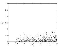
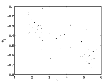
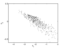
Our ABC algorithm used two summary statistics of the data: $S_{1}(y)=\sum_{(i,j)\in\mathbf{N}}y_{i}y_{j}$ (the number of equivalently valued neighbours) and $S_{2}(y)=\sum_{i}y_{i}$ (the magnetisation). In the adaptive ABC-SMC algorithm, we choose that 70% of the particles were given non-zero weight at each iteration. Points from $p(\theta_{x},\theta_{y}|y)$ using this method, which was terminated at $n=12$, are shown in figure 1b: the posterior mass is distributed around the areas where $\theta_{x}$ is small and/or $\theta_{y}$ is small. It is clear that this posterior will pose a significant challenge to DA: in order to explore the posterior fully it is necessary to sample both large and small values of $\theta_{x}$, and moving from one side of the critical value of $\theta_{x}$ to the other is difficult due to the dependence between $x$ and $\theta_{x}$. Points from $p(\theta_{x},\theta_{y}|y)$ using DA, in which we chose $s=1$ and $L=10^{5}$, are shown in figure 1c. The posterior dependency between $\theta_{x}$ and $x$, and the inefficiency of the updates on $p(x|\theta,y)$ (even when using $10^{5}$ sweeps of the Gibbs sampler at every iteration), inhibit the sampler from moving below the critical value of $\theta_{x}$.

In this implementation of the marginal PMCMC algorithm, we use hot coupling for the SMC sampler updates, adding a single edge at each target (this results in a total of 82 targets, giving approximately 1200 particles). The simlated points are shown in figure 1d: the sampler has explored the whole posterior, with no evidence of difficulty in passing the critical value of $\theta_{x}$. Figure 1e shows the trace plot of $S_{1}(x)$ for both the DA and the PMCMC methods, illustrating that the PMCMC approach enables exploration of the $x$ space, whereas DA only explores graphs that correspond to a large value of $\theta_{x}$. In both the DA and PMCMC extended exchange algorithms, we use $B=100$ intermediate targets in the annealed IS: fewer intermediate targets can result in poor estimation of the ratio of normalising constants, and therefore inefficiency in both algorithms. If the original exchange algorithm is used ($B=1$), the results from the PMCMC method do not look dissimilar to those produced by the DA method: when there is a proposed change in $\theta_{x}$ that crosses the critical value, the move is rejected since the proposed $u\sim f(.|\theta^{*})$ has a small probability of being generated under $\theta$.

The dominating factor in the computational cost of each algorithm is in the Gibbs sampler for the simulation from the $x$ space (with the target of either $p(x|\theta)$ or $p(x|\theta,y)$). For each iteration of the DA or PMCMC algorithm $10^{5}$ sweeps of the Gibbs sampler are performed at each iteration of the MCMC (along with an additional $10^{3}$ for the exchange algorithm), so the total cost of our run is approximately $5\times 10^{8}$ sweeps. For each target of the ABC-SMC $10^{7}$ sweeps are performed, so the total computational cost is $1.2\times 10^{8}$ sweeps.

Figure 1: Results for Bayesian parameter estimation in a hidden Ising model.

(a) Observed data.

(b) Points from the posterior produced by the ABC-SMC algorithm.

(c) Points simulated from the posterior using the DA exchange algorithm.

(d) Points simulated from the posterior using the exchange marginal PMCMC algorithm.

(e) Trace plot of the statistic $S_{1}(x)$, the number of identical neighbours in the hidden field $x$, for the DA (black) and the PMCMC (grey) algorithms.

4.3 Social Network Data

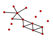
We consider the application of our methods to the Florentine family business graph studied in Caimo and Friel (2011), shown in figure 2a. We begin by assuming the network $x$ is directly observed and use exactly the model for the data as that used in Caimo and Friel (2011): using an ERGM (equation (5)) with $S_{1}(x)=\sum_{i<j}x_{ij}$ (the number of edges) and $S_{2}(x)=\sum_{i<j<k}x_{ik}x_{jk}$ (the number of 2-stars) , and prior on $\theta_{x}=(\theta_{1},\theta_{2})$ as $\theta_{x}\sim\mathcal{N}(0,30I_{2})$.

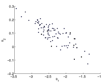
We begin by examining ABC as a direct alternative to the MCMC approach in Caimo and Friel (2011) (the DA and PMCMC approaches are not applicable here since there is no latent space). We use the statistics $S_{1}$ and $S_{2}$ as our summary of the data, and since these statistics are sufficient, when $\epsilon=0$ the ABC posterior is equivalent to the true posterior. In this implementation the scale of the target changes dramatically across the iterations (since the posterior is significantly tighter than the prior), thus we adaptively choose the proposal variance in the MH move, so that at iteration $n$, the variance is $2\widehat{\Sigma}_{n-1}$ where $\widehat{\Sigma}_{n-1}$ is the sample variance of the particles at iteration $n-1$ (as in Robert et al. (2011)). We choose that 50% of the particles were given non-zero weight at each iteration. The ABC-SMC terminated at $n=16$, and weighted points drawn from $p(\theta_{1},\theta_{2}|y)$ using this method are shown in figure 2b. These points are in good agreement with the shape of the posterior shown in Caimo and Friel (2011). We note that the “population” nature of the SMC algorithm acts as a substitute for the population MCMC method employed in that paper.

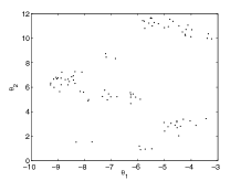
Now consider the case where it is assumed that the observed graph, now denoted by $y$, is a noisy observation of some underlying graph $x$. Specifically, we use the model in equation (6), which account for noisy observations of the edges of the underlying graph. We use a generalisation of the model described above, defined on the extended parameter $\theta=(\theta_{1},\theta_{2},\theta_{y})$ with the same priors on $\theta_{1}$ and $\theta_{2}$, and with a prior of $\theta_{y}\sim\mathcal{U}[0,100]$ on the additional parameter $\theta_{y}$. Note that the data itself does not suggest that this model is particularly suitable: it is chosen simply to highlight the computational problems that can result in the presence of a latent ERGM. We use the same ABC-SMC algorithm as above, using the same summary statistics (which are now not sufficient). The ABC-SMC again terminated at $n=16$, and weighted points simulated from $p(\theta_{1},\theta_{2}|y)$ using this method are shown in figure 2c. One of the limitations of ABC is evident here: since the statistics are not sufficient, it is difficult to assess how accurate the approximation to the true posterior is, even though we have $\epsilon=0$. We applied the DA algorithm and PMCMC algorithms to the same model that assumes the data is noisy (including the parameter $\theta_{y}$). In the DA algorithm we chose $s=10$ and $L=10^{4}$ and points generated from $p(\theta_{1},\theta_{2}|y)$ are shown in figure 2d. The posterior sample produced by this sampler was highly dependant on the initial point. In this particular example, when the initial value of $x$ is the complete graph (where all edges are present), the chain gets stuck in this state, which is highly correlated a posteriori with a small value of $\theta_{y}$. Again, the inefficiency of the updates on $x$ and the dependency between $x$ and $\theta$ is seen to lead to the poor performance of the DA approach.

In addition to comparing the PMCMC approach to DA, we also compare the original IS based pseudo-marginal approach to the more general PMCMC approach in order to observe the benefit of using an SMC sampler in sampling the $x$ space. Specifically, we compare IS with $10^{4}$ importance points drawn using a uniform distribution independently on each edge, with the SMC sampler with tempering using 1000 targets and 10 particles. Figures 2e and 2f respectively illustrate the PMCMC results using these two schemes. The performance of the IS based technique is poor since the importance proposal is poor and does not provide an accurate estimate of the normalising constant $Z(\theta)p(y|\theta)$. The performance of the tempering SMC based EMPMCMC is significantly better than both the IS and DA approaches, with convergence to the region shown in figure 2f regardless how the MCMC is initialised. This lack of dependence on initial conditions, and the free exploration of the $x$ and $\theta_{y}$ space that is allowed by the method, provide some evidence that this method has found the true posterior.

In the DA and PMCMC extended exchange algorithms, we use 1000 intermediate targets in the extended exchange algorithm: again we find that fewer intermediate targets results in poor estimation of the ratio of normalising constants and thus inefficient MCMC algorithms.

Again, the dominating factor in the computational cost of each algorithm is in the Gibbs sampler for the simulation from the $x$ space. In this case, for each iteration of the DA or PMCMC algorithm $10^{4}$ sweeps of the Gibbs sampler are performed at each iteration of the MCMC (along with an additional $10^{3}$ for the exchange algorithm), so the total cost of our run is approximately $5\times 10^{7}$ sweeps. For each target of the ABC-SMC $10^{7}$ sweeps are performed, so the total computational cost is $1.6\times 10^{8}$ sweeps. The method of Caimo and Friel (2011) is relatively cheap compared to ABC-SMC, with the only simulation from the $x$ space being carried out as part of the exchange algorithm (which costs $10^{3}$ sweeps).

Figure 2: Results for Bayesian parameter estimation in a hidden ERGM.

(a) Observed data.

(b) Points from the posterior (with no observation error) produced by the ABC-SMC algorithm.

(c) Points from the posterior produced by the ABC-SMC algorithm.

(d) Points simulated from the posterior using the DA exchange algorithm.

(e) Importance sampling based pseudo-marginal approach, with the exchange algorithm.

(f) Points simulated from the posterior using the exchange marginal PMCMC algorithm containing an SMC sampler.

5   DISCUSSION

Bayesian parameter estimation for latent MRFs can face computational difficulties using standard methodology since the DA approach can be extremely inefficient. We have described two methods, ABC and PMCMC that can offer an alternative in situations where DA is not suitable.

ABC is currently particularly popular for addressing missing data problems, and we apply it for the first time to inference in ERGMs as a method for avoiding the intractable normalising constant. We also provide a theoretical justification for the use of MCMC for inexact simulation from the likelihood, as is required in many MRF models, within ABC-MCMC. However, we observe the usual limitations of ABC in cases where sufficient statistics are not available: namely that an approximation that is difficult to quantify is introduced.

Marginal PMCMC offers an effective means of bypassing the potential inefficiency of DA and our results indicate that this method is a promising approach to parameter estimation in these models. We note the large computational cost of these methods, especially when sampling from a high dimensional latent space. As such, routine use of the method will usually only be possible when accompanied by an efficient implementation, possibly on parallel computing architectures such as graphics cards or cloud computing resources. Given the increase in popularity of this hardware, the PMCMC methodology offers a promising avenue for use on more realistic applications in the near future. The key aspect of PMCMC is the use of an SMC sampler for sampling from the $x$ space. Although we have focussed on parameter estimation, our results (and those of Hamze and de Freitas (2005)) indicate that SMC samplers have an important role to play in simulating from MRFs, both when the parameters are known and unknown. These methods have not been used before in the ERGM literature, and address some of the known problems with MCMC described in Snijders (2002).

We follow previous work in using the exchange algorithm to account for the intractable normalising constant, and give theoretical justification for the use of approximate exchange algorithms where MCMC as a substitute for exact simulation from the likelihood. In application, we find the use of the extended version of the exchange algorithm described in Murray et al. (2006) to be essential to ensure the MCMC can move freely in the problems we consider.

Appendix A: Target Distribution of Exchange Marginal PMCMC

This appendix establishes that the EMPMCMC algorithm in section 2.2.3 of the paper has the desired target density of $p(\theta|y)$. The proof requires the description of the extended target and proposal distribution used as a consequence of the use of the SMC sampler within the algorithm.

For ease of exposition, we express the algorithm in a slightly different form to that in the main text, including the prior $p(\theta)$ within the SMC sampler. The $i$’th iteration of the algorithm is then:

1. Draw $\theta^{*}\sim q(.|\theta(i-1))$ and $u\sim f(.|\theta^{*})$.

2. Run an SMC sampler on the $x$ space, with the final (unnormalised) distribution as $\pi_{T}(x)=p(\theta)\gamma(x,y|\theta^{*})$ in order to obtain the particle approximation $\widehat{p}(x|\theta^{*},y)$ to the distribution $\widehat{p}(x|\theta^{*},y)=p(\theta^{*})\gamma(x,y|\theta^{*})/Z(\theta^{*})p(\theta^{*},y)$ and an estimate $\widehat{\phi}(\theta^{*},y)$ of its normalising constant, $\phi(\theta^{*},y):=Z(\theta^{*})p(\theta^{*},y)$.

3. Sample a single point $x^{*}$ from $\widehat{p}(.|\theta^{*},y)$.

4. Let $(\theta(i),\theta^{*}(i),x(i),\widehat{\phi}(i),u(i))=(\theta^{*},\theta(i-1),x^{*},\widehat{\phi}(\theta^{*},y),u)$ with probability:

   $$1\wedge\frac{\widehat{\phi}(\theta^{*},y)q(\theta|\theta^{*})\gamma(u|\theta)}{\phi(i-1)q(\theta^{*}|\theta)\gamma(u|\theta^{*})},$$

   otherwise set $(\theta(i),\theta^{*}(i),x(i),\widehat{\phi}(i),u(i))=(\theta(i-1),\theta^{*}(i-1),x(i-1),\widehat{\phi}(i-1),u(i-1))$.

In advance of the proof we also make some definitions relating to the use of the SMC sampler (using $\theta$ rather than $\theta^{*}$ throughout to simplify the notation). We define $\pi_{k}^{\theta}(x_{k})=\gamma_{k}^{\theta}(x_{k})/\phi_{k}(\theta)$ (for $k=1,...,T$) to be the sequence of targets used in the SMC sampler. In our case, we take $\gamma_{T}^{\theta}(x_{T})=p(\theta)\gamma(x_{T},y|\theta)$ and $\phi_{T}(\theta)=\phi(\theta,y)$, so that $\pi_{T}^{\theta}(x_{k})=p(x|\theta,y)$. The underlying construction of the SMC sampler is such that it targets the artificially constructed sequence of distributions $\widetilde{\pi}_{k}^{\theta}(x_{1:k})=\widetilde{\gamma}_{k}^{\theta}(x_{1:k})/\phi_{k}(\theta)$ (for $k=1,...,T$), with

$$\widetilde{\gamma}_{k}^{\theta}(x_{1:k})=\gamma_{k}^{\theta}(x_{k})\prod_{j=1}^{k-1}L_{j}^{\theta}(x_{j+1},x_{j}).$$

The SMC sampler generates a weighted importance sample from each extended target $\widetilde{\pi}_{k}^{\theta}(x_{1:k})$ in succession. We denote the state of the $p$’th particle at the $k$’th target by $x_{1:k}^{p}$ (the joint state of all particles at the $k$th target is denoted by $x_{1:k}$). At the $k$’th target, the particles are: resampled; moved using a transition kernel; then weighted.

To describe the resampling step, we introduce the distribution $r(a_{k-1}|w_{k-1})$, with $w_{k-1}$ denoting the weights of the particles at target $k-1$ and $a_{k-1}=(a_{k-1}^{1},...,a_{k-1}^{P})$ with $a_{k-1}^{p}$ giving the index of the “parent” particle of “child” particle $x_{1:k}^{p}$. This operation can be interpreted as the process by which child particles at target $k$ choose their parent particles from the population at target $k-1$. For the proof we also need to define, for $k=1,...,T$ and $p=1,...,P$, the index $b_{k}^{p}$ which the ancestor particle of $x_{1:T}^{p}$ at target $k$ had at that time.

Let $M_{1}(x_{1})$ be the initial proposal density and $M_{k}(x_{k-1},x_{k})$ for $k=2,...,T$ be the transition kernels used at each target. The weighting step, applied to the $p$’th particle at the $k$’th target after the resampling and move steps, finds the unnormalised weight $\widetilde{w}_{k}^{p}$ of the particle at the current target:

$$\widetilde{w}_{k}^{p}=\frac{\gamma_{k}^{\theta}(x_{k})L_{k-1}^{\theta}(x_{k},x_{k-1}^{a_{k-1}^{p}})}{\gamma_{k-1}^{\theta}(x_{k-1}^{a_{k-1}^{p}})M_{k}(x_{k-1}^{a_{k-1}^{p}},x_{k})}.$$ (15)

The weight is then normalised:

$$w_{k}^{p}=\frac{\widetilde{w}_{k}^{p}}{\sum_{p=1}^{P}\widetilde{w}_{k}^{p}}.$$

An approximation to the target $p(x|\theta,y)$ is then given by

$$\widehat{p}(dx|\theta,y)=\sum_{p=1}^{P}w_{T}^{p}\delta_{x_{T}^{p}}(dx)$$

where $\delta$ is the Dirac delta function, with an estimate of its normalising constant given by

$$\widehat{\phi}(\theta,y)=\prod_{k=1}^{T}\left[\frac{1}{P}\sum_{p=1}^{P}\widetilde{w}_{T}^{p}\right].$$

In advance of the theorem, we introduce the joint density of the variables generated by the SMC algorithm that uses $P$ particles and $T$ targets, defined on the space $\mathcal{X}^{TP}\times\left\{1,...,P\right\}^{(T-1)P}$:

$$\psi^{\theta}(x_{1},...,x_{T},a_{1},...,a_{T-1}) := \psi^{\theta}(x_{1})\prod_{k=2}^{T}\psi^{\theta}(a_{k-1}|x_{k-1})\psi^{\theta}(x_{k}|x_{k-1},a_{k-1})$$

$$= \left(\prod_{p=1}^{P}M_{1}^{\theta}\left(x_{1}^{p}\right)\right)\prod_{k=2}^{T}\left(r(a_{k-1}|w_{k-1})\prod_{p=1}^{P}M_{k}^{\theta}\left(x_{k-1}^{a_{k-1}^{p}},x_{k}^{p}\right)\right).$$

Theorem 1.

Let $O_{k}^{p}:=\sum_{j=1}^{P}\mathbb{I}(a_{k}^{j}=p)$ be the number of offspring of particle $p$ at target $k$. If for any $p=1,...,P$ and $k=1,...,T$ the resampling scheme satisfies

$$\mathbb{E}[O_{k}^{p}]=Pw_{k}^{p},$$

(i.e., it is unbiased) and also that

$$r(a_{k}^{p}=m|w_{k})=w_{k}^{m},$$ (16)

then the EMPMCMC algorithm is an MCMC algorithm targeting a joint distribution that admits $p(\theta,x|y)$ as a marginal.

Proof.

The structure of the proof is as follows. We first fully describe the target and proposal densities used in the marginal PMCMC algorithm, then combine these with the density of the $u$ variable generated for the exchange algorithm, and show that the EMPMCMC algorithm performs a deterministic “swap” move on this extended target.

To begin, on the space $\mathcal{E}:=\Theta\times\mathcal{X}^{TP}\times\left\{1,...,P\right\}^{(T-1)P+1}$, we define the proposal and target for a marginal PMCMC algorithm. To simply the notation, let $E=(\theta,v,x_{1},...,x_{T},a_{1},...,a_{T-1})$ and $E^{*}=(\theta^{*},v^{*},x_{1}^{*},...,x_{T}^{*},a_{1}^{*},...,a_{T-1}^{*})$. The proposal is then

$$q^{N}(\theta,E^{*}) := q(\theta^{*}|\theta)w_{T}^{*v^{*}}\psi^{\theta^{*}}(x_{1}^{*},...,x_{T}^{*},a_{1}^{*},...,a_{T-1}^{*})$$

where the weight $w_{T}^{*v^{*}}$ is present due to the sampling of the index $v^{*}$ to generate $x^{*}$ from the particle approximation $\widehat{p}(dx|\theta,y)$. The target density is given by

$$\tilde{\pi}^{N}(E) := \frac{p(\theta,x_{T}^{v}|y)\prod_{k=2}^{T}L_{k-1}^{\theta}(x_{k}^{b_{T}^{v}},x_{k-1}^{b_{T}^{v}})}{P^{T}}\frac{\psi^{\theta}(x_{1},...,x_{T},a_{1},...,a_{T-1})}{M_{1}^{\theta}\left(x_{1}^{b_{1}^{v}}\right)\prod_{k=2}^{T}r(b_{k-1}^{v}|w_{k-1})M_{k}^{\theta}\left(x_{k-1}^{b_{k-1}^{v}},x_{k}^{b_{k}^{v}}\right)},$$

which has the desired $p(\theta,x|y)$ as a marginal.

Now to derive the acceptance probability of the EMPMCMC algorithm, we express the algorithm in terms of a deterministic swap move on the following extended target:

$$\check{\pi}(E,E^{*},u):=\tilde{\pi}^{N}(E)q^{N}(\theta,E^{*})\gamma(u|\theta^{*})/Z(\theta^{*}).$$

Specifically, at each iteration of the algorithm, we apply the transformation $T:\mathcal{E}\times\mathcal{E}\times\mathcal{X}\rightarrow\mathcal{E}\times\mathcal{E}\times\mathcal{X}$ defined by

$$T(E,E^{*},u)=(E^{*},E,u).$$

The acceptance probability of this move is given by

$$1\wedge\frac{\check{\pi}(T(E,E^{*},u))}{\check{\pi}(E^{*},E,u)} = 1\wedge\frac{\tilde{\pi}^{N}(E^{*})}{q^{N}(\theta,E^{*})}\frac{q^{N}(\theta^{*},E)}{\tilde{\pi}^{N}(E)}\frac{\gamma(u|\theta)Z(\theta^{*})}{\gamma(u|\theta^{*})Z(\theta)}.$$ (17)

The term $\tilde{\pi}^{N}(E)/q^{N}(\theta^{*},E)$ simplifies as follows:

$$\frac{\tilde{\pi}^{N}(E)}{q^{N}(\theta^{*},E)} = \frac{1}{P^{T}}\frac{p(\theta,x_{T}^{v}|y)\prod_{k=2}^{T}L_{k-1}^{\theta}(x_{k}^{b_{T}^{v}},x_{k-1}^{b_{T}^{v}})}{q(\theta|\theta^{*})w_{T}^{v}M_{1}^{\theta}\left(x_{1}^{b_{1}^{v}}\right)\prod_{k=2}^{T}r(b_{k-1}^{v}|w_{k-1})M_{k}^{\theta}\left(x_{k-1}^{b_{k-1}^{v}},x_{k}^{b_{k}^{v}}\right)}$$ (18)

$$= \frac{p(\theta,x_{T}^{v}|y)\prod_{k=2}^{T}L_{k-1}^{\theta}(x_{k}^{b_{T}^{v}},x_{k-1}^{b_{T}^{v}})}{q(\theta|\theta^{*})M\left(x_{1}^{b_{1}^{v}}\right)\prod_{k=2}^{T}M_{k}^{\theta}\left(x_{k-1}^{b_{k-1}^{v}},x_{k}^{b_{k}^{v}}\right)}\frac{\frac{1}{P^{T}}}{\prod_{k=1}^{T}w_{k}^{b_{k}^{v}}}$$

$$= \frac{p(\theta,x_{T}^{v}|y)\prod_{k=2}^{T}L_{k-1}^{\theta}(x_{k}^{b_{T}^{v}},x_{k-1}^{b_{T}^{v}})}{\phi(\theta,y)q(\theta|\theta^{*})M\left(x_{1}^{b_{1}^{v}}\right)\prod_{k=2}^{T}M_{k}^{\theta}\left(x_{k-1}^{b_{k-1}^{v}},x_{k}^{b_{k}^{v}}\right)}\frac{\frac{1}{P^{T}}\prod_{k=1}^{T}\sum_{p=1}^{P}\tilde{w}_{k}^{p}}{\prod_{k=1}^{T}\widetilde{w}_{k}^{b_{k}^{v}}}$$

$$= \frac{p(\theta)\gamma(x_{T}^{v},y|\theta)\prod_{k=2}^{T}L_{k-1}^{\theta}(x_{k}^{b_{T}^{v}},x_{k-1}^{b_{T}^{v}})}{q(\theta|\theta^{*})M\left(x_{1}^{b_{1}^{v}}\right)\frac{\gamma_{1}(x_{1}^{b_{1}^{v}})}{M_{1}(x_{1}^{b_{1}^{v}})}\prod_{k=2}^{T}M_{k}^{\theta}\left(x_{k-1}^{b_{k-1}^{v}},x_{k}^{b_{k}^{v}}\right)\frac{\gamma_{k}^{\theta}(x_{k}^{b_{k}^{v}})L_{k-1}^{\theta}(x_{k}^{b_{k}^{v}},x_{k-1}^{b_{k-1}^{v}})}{\gamma_{k-1}^{\theta}(x_{k-1}^{b_{k-1}^{v}})M_{k}(x_{k-1}^{b_{k-1}^{v}},x_{k}^{b_{k}^{v}})}}\frac{\widehat{\phi}(\theta,y)}{p(y)Z(\theta)}$$

$$= \frac{\widehat{\phi}(\theta,y)}{q(\theta|\theta^{*})p(y)Z(\theta)},$$

using equations (15) and (16).

Now, substituting equation (18) into equation (17), we obtain

$$1\wedge\frac{\check{\pi}(T(E,E^{*},u))}{\check{\pi}(E^{*},E,u)} = 1\wedge\frac{\widehat{\phi}(\theta^{*},y)}{q(\theta^{*}|\theta)p(y)Z(\theta^{*})}\frac{q(\theta|\theta^{*})p(y)Z(\theta)}{\widehat{\phi}(\theta,y)}\frac{\gamma(u|\theta)Z(\theta^{*})}{\gamma(u|\theta^{*})Z(\theta)}$$

$$= 1\wedge\frac{\widehat{\phi}(\theta^{*},y)}{\widehat{\phi}(\theta,y)}\frac{q(\theta|\theta^{*})}{q(\theta^{*}|\theta)}\frac{\gamma(u|\theta)}{\gamma(u|\theta^{*})},$$

as required. ∎

Appendix B: Convergence of Approximate Algorithms

In the appendix we prove the convergence of MCMC algorithms that take the following form. We note that the assumptions used for the proof are relatively strong, and are not widely applicable. However, it likely that similar (weaker) results exist under weaker assumptions: the results in this paper are intended as the first steps towards future work that would obtain results that hold more generally.

Suppose that we have an “exact” MCMC algorithm, using transition kernel

$$K((\theta,u),(\theta^{*},u^{*}))=q(\theta^{*}|\theta)\pi_{\theta^{*}}(u^{*})\alpha((\theta,u),(\theta^{*},u^{*}))+\delta_{\theta,u}(\theta^{*},u^{*})r(\theta,u),$$

where $\alpha((\theta,u),(\theta^{*},u^{*}))$ is such that $K$ is an MCMC kernel that has an invariant distribution of $\pi(\theta,u)=\pi(\theta)\pi_{\theta}(u)$ and

$$r(\theta,u)=1-\int_{\theta^{*},u^{*}}q(\theta^{*}|\theta)\pi_{\theta^{*}}(u^{*})\alpha((\theta,u),(\theta^{*},u^{*}))d\theta^{*}du^{*}.$$

The SAV method takes this precise form. The theorem below characterises the invariant distribution (where it exists), and the convergence rate, of the “approximate” MCMC algorithm given by the kernel

$$\widetilde{K}_{M}((\theta,u),(\theta^{*},u^{*}))=q(\theta^{*}|\theta)L_{\theta^{*}}^{M}(v_{0},u^{*})\alpha((\theta,u),(\theta^{*},u^{*}))+\delta_{\theta,u}(\theta^{*},u^{*})\widetilde{r}(\theta,u),$$

where $L_{\theta^{*}}^{M}(v_{0},u^{*})$ represents $M$ iterations of an MCMC kernel with invariant distribution $\pi_{\theta^{*}}(u^{*})$, beginning at an arbitrary fixed initial value $v_{0}\in\mathcal{X}$ and

$$\widetilde{r}(\theta,u)=1-\int_{\theta^{*},u^{*}}q(\theta^{*}|\theta)L_{\theta^{*}}^{M}(v_{0},u^{*})\alpha((\theta,u),(\theta^{*},u^{*}))d\theta^{*}du^{*}.$$

The same argument can be used the prove equivalent properties of the approximate exchange and ABC-MCMC algorithms described in the main text. In the exact versions of these algorithms the target distributions and transition kernels have slightly different forms to that of the SAV method:

• the exchange algorithm has the target distribution given in the main text, and the proposal additionally contains the deterministic “swap” move described in the main text;

• the ABC-MCMC algorithm can be seen to target $\pi(\theta)\pi_{\theta}(u)\pi_{\epsilon}(u|y)$ (changing the notation to be consistent with that used in the proof), with the proposal taking the form $q(\theta^{*}|\theta)\pi_{\theta^{*}}(u^{*})$.

These differences also result in a different acceptance probability to that used in the SAV algorithm, but have no impact on the structure of the proof of the theorem.

Throughout the theorem and proof, $\left\|.\right\|$ represents the total variation norm.

Theorem 2.

Suppose the Metropolis-Hastings kernel $K$ is uniformly ergodic, i.e. there exists $C_{K}\in(0,\infty)$ and $\rho_{K}\in(0,1)$, such that for any $(\theta_{0},u_{0})\in\Theta\times\mathcal{X}$ and $n\in\mathbb{N}$

$$\left\|K^{n}((\theta_{0},u_{0}),.)-\pi(.)\right\|\leq C_{K}\rho_{K}^{n};$$

$L_{\theta^{*}}$ is geometrically ergodic for all $\theta^{*}\in\Theta$, i.e. for all $\theta^{*}\in\Theta$, there exists $C_{L}(v_{0},\theta^{*})\in(0,\infty)$ and $\rho_{L}\in(0,1)$, such that for $\pi_{\theta^{*}}$-a.e. $v_{0}\in\mathcal{X}$ and $n\in\mathbb{N}$

$$\left\|L_{\theta^{*}}^{n}(v_{0},.)-\pi_{\theta^{*}}(.)\right\|\leq C_{L}(v_{0})\rho_{L}^{n};$$

uniformly in $\theta^{*}$. Additionally, suppose that for some $D>0$, $\sup_{\theta,\theta^{\prime}}q(\theta^{\prime}|\theta)\leq D$, where $q$ is the proposal used in the kernel $K$, and for any $M\geq 1$ there exists a distribution $\widetilde{\pi}_{M}$ on $\Theta\times\mathcal{X}$ such that $\widetilde{\pi}_{M}\widetilde{K}_{M}=\widetilde{\pi}_{M}$.

Then for any $\epsilon\in(0,\rho_{K}^{-1}-1)$ there exists $M_{0}\in\mathbb{N}$, $\widetilde{\rho}_{K}\in(\rho,\rho(1+\epsilon)]\subset(\rho,1)$ and $\widetilde{C}\in(0,\infty)$ such that for all $M\geq M_{0}$, $(\theta_{0},u_{0})\in\Theta\times\mathcal{X}$ and $n\geq 1$,

$$\left\|\widetilde{K}_{M}^{n}((\theta_{0},u_{0}),.)-\widetilde{\pi}_{M}(.)\right\|\leq\widetilde{C}\widetilde{\rho}_{K}^{n},$$ (19)

$$\left\|\pi(.)-\widetilde{\pi}_{M}(.)\right\|\leq C_{K}\frac{\epsilon}{1-\rho_{K}}.$$ (20)

Proof.

To begin, for any $\theta,u\in\Theta\times\mathcal{X}$ and $n\in\mathbb{N}$,

$$\left\|\widetilde{K}_{M}^{n}((\theta,u),.)-K^{n}((\theta,u),.)\right\| \leq \sum_{i=0}^{n-1}\left\|\widetilde{K}_{M}^{n-i-1}((\theta,u),(K-\widetilde{K}_{M})(K^{i}-\pi)(.))\right\|$$ (21)

$$\leq C_{K}\sup_{\theta,u}\left\|K((\theta,u),.)-\widetilde{K}_{M}((\theta,u),.)\right\|\sum_{i=0}^{n-1}\rho_{K}^{i}$$

$$\leq \frac{C_{K}}{1-\rho_{K}}\sup_{\theta,u}\left\|K((\theta,u),.)-\widetilde{K}_{M}((\theta,u),.)\right\|$$

We now bound the final term on the right hand side. We have:

$$\sup_{\theta,u}\left\|K((\theta,u),.)-\widetilde{K}_{M}((\theta,u),.)\right\| = \sup_{\theta,u}\sup_{fs.t.|f|\leq 1}\left|\int K((\theta,u),(d\theta^{\prime},du^{\prime}))f(\theta^{\prime},u^{\prime})-\int\tilde{K}_{M}((\theta,u),(d\theta^{\prime},du^{\prime}))f(\theta^{\prime},u^{\prime})\right|$$

$$= \sup_{\theta,u}\sup_{fs.t.|f|\leq 1}\left|\int\left[q(d\theta^{\prime}|\theta)\pi_{\theta^{\prime}}(du^{\prime})\alpha((\theta,u),(d\theta^{\prime},du^{\prime}))+\delta_{\theta,u}(d\theta^{\prime},du^{\prime})r(\theta,u)\right]f(\theta^{\prime},u^{\prime})\right.$$

$$\quad\left.-\int\left[q(d\theta^{\prime}|\theta)L_{\theta^{\prime}}^{M}(v_{0},du^{\prime})\alpha((\theta,u),(d\theta^{\prime},du^{\prime}))+\delta_{\theta,u}(d\theta^{\prime},du^{\prime})\widetilde{r}(\theta,u)\right]f(\theta^{\prime},u^{\prime})\right|$$

$$\leq \sup_{\theta,u}\sup_{fs.t.|f|\leq 1}\left|\int\left[q(d\theta^{\prime}|\theta)\alpha((\theta,u),(d\theta^{\prime},du^{\prime}))f(\theta^{\prime},u^{\prime})\left\{\pi_{\theta^{\prime}}(du^{\prime})-L_{\theta^{\prime}}^{M}(v_{0},du^{\prime})\right\}\right]\right|$$

$$\qquad+\sup_{\theta,u}\sup_{fs.t.|f|\leq 1}\left|f(\theta,u)\left\{r(\theta,u)-\widetilde{r}(\theta,u)\right\}\right|$$

$$\leq \sup_{\theta,u}\sup_{fs.t.|f|\leq 1}\int\left|q(d\theta^{\prime}|\theta)\right|\left|\alpha((\theta,u),(d\theta^{\prime},du^{\prime}))\right|\left|f(\theta^{\prime},u^{\prime})\right|\left|\pi_{\theta^{\prime}}(du^{\prime})-L_{\theta^{\prime}}^{M}(v_{0},du^{\prime})\right|$$

$$\qquad+\sup_{\theta,u}\sup_{fs.t.|f|\leq 1}\left|f(\theta,u)\right|\left|r(\theta,u)-\widetilde{r}(\theta,u)\right|$$

$$\leq \int D\left|\pi_{\theta^{\prime}}(du^{\prime})-L_{\theta^{\prime}}^{M}(v_{0},du^{\prime})\right|+\sup_{\theta,u}\left|r(\theta,u)-\widetilde{r}(\theta,u)\right|$$

$$\leq DC_{L}(v_{0})\rho_{L}^{M}+\sup_{\theta,u}\left|r(\theta,u)-\widetilde{r}(\theta,u)\right|$$

using the geometric ergodicity of $L_{\theta^{*}}$ for every $\theta^{*}\in\Theta$. Using this property again, for the final term we have:

$$\sup_{\theta,u}\left|r(\theta,u)-\widetilde{r}(\theta,u)\right| = \sup_{\theta,u}\left|\int_{\theta^{*},u^{*}}q(\theta^{*}|\theta)\alpha\left((\theta,u),(\theta^{*},u^{*})\right)\right.$$

$$\qquad\left.\left(L_{\theta^{*}}^{M}(v_{0},u^{*})-\pi_{\theta^{*}}(u^{*})\right)d\theta^{*}du^{*}\right|$$

$$\leq C_{L}(v_{0})\rho_{L}^{M}\sup_{\theta,u}\left|\int_{\theta^{*},u^{*}}q(\theta^{*}|\theta)\alpha\left((\theta,u),(\theta^{*},u^{*})\right)d\theta^{*}du^{*}\right|$$

$$\leq C_{L}(v_{0})\rho_{L}^{M}.$$

Combining these results we obtain

$$\sup_{(\theta,u)\in\Theta\times\mathcal{X}}\left\|K((\theta,u),.)-\widetilde{K}_{M}((\theta,u),.)\right\|\leq(D+1)C_{L}(v_{0})\rho_{L}^{M}.$$

Using this result, and the uniform ergodicity of $K$, we obtain that for any $(\theta,u),(\vartheta,v)\in\Theta\times\mathcal{X}$

$$\left\|\widetilde{K}_{M}^{n}((\theta,u),.)-\widetilde{K}_{M}^{n}((\vartheta,v),.)\right\| \leq \left\|\widetilde{K}_{M}^{n}((\theta,u),.)-K_{M}^{n}((\theta,u),.)\right\|+\left\|K_{M}^{n}((\vartheta,v),.)-\widetilde{K}_{M}^{n}((\vartheta,v),.)\right\|$$

$$\qquad+\left\|K_{M}^{n}((\theta,u),.)-K_{M}^{n}((\vartheta,v),.)\right\|$$

$$\leq 2\frac{C_{K}}{1-\rho_{K}}(D+1)C_{L}(u_{0})\rho_{L}^{M}+C_{K}\rho_{K}^{n}.$$

Now define

$$\widetilde{\rho}_{K}:=\rho_{K}\sqrt[n]{C_{K}\left(1+2\frac{\rho_{L}^{M}\rho_{K}^{-n}}{1-\rho}(D+1)C_{L}(v_{0})\right)}\leq\rho_{K}\sqrt[n]{C_{K}}\left(1+2\frac{\rho_{L}^{M}\rho_{K}^{-n}}{1-\rho}(D+1)C_{L}(v_{0})\right).$$

Choose $\epsilon\in(0,\rho_{K}-1)$ and let $n\in\mathbb{N}$ be such that $\sqrt[n]{C_{K}}\leq\sqrt{1+\epsilon}$ and $M_{1}\in\mathbb{N}$ such that

$$1+2\frac{\rho_{L}^{M_{1}}\rho_{K}^{-n}}{1-\rho}(D+1)C_{L}(v_{0})\leq\sqrt{1+\epsilon}.$$

We then have that $\widetilde{\rho}_{K}\leq\rho_{K}(1+\epsilon)<1$ for $M>M_{1}$, and equation 19 follows.

Then from equation 21 we have that for any $n\geq 1$

$$\left\|\pi\widetilde{K}_{M}^{n}((\theta,u),.)-\pi K^{n}((\theta,u),.)\right\| \leq \sum_{i=0}^{n-1}\left\|\pi\left(\widetilde{K}_{M}^{n-i-1}((\theta,u),(K-\widetilde{K}_{M})(K^{i}-\pi)(.))\right)\right\|$$

$$\leq C_{K}(D+1)C_{L}(u_{0})\rho_{L}^{M}\sum_{i=0}^{n-1}\rho_{K}^{i}$$

$$\leq \frac{C_{K}}{1-\rho_{K}}(D+1)C_{L}(v_{0})\rho_{L}^{M}.$$

So for any $\varepsilon>0$, we can chose $M_{2}\in\mathbb{N}$ such that $(D+1)C_{L}(u_{0})\rho_{L}^{M_{2}}\leq\varepsilon$, so that

$$\left\|\pi\widetilde{K}_{M}^{n}((\theta,u),.)-\pi K^{n}((\theta,u),.)\right\|\leq\frac{C_{K}\varepsilon}{(1-\rho_{K})}.$$

Using $\left\|\pi-\widetilde{\pi}_{M}\right\|=\lim_{n\rightarrow\infty}\left\|\pi K_{M}^{n}-\widetilde{\pi}_{M}\widetilde{K}_{M}^{n}\right\|$ and choosing $M_{0}=M_{1}\vee M_{2}$ the proof is completed. ∎

We note that the same argument may be used to obtain the same result where $L_{\theta^{*}}$ is allowed to use the value of $u$ generated at the previous iteration, as long as $L_{\theta^{*}}$ is uniformly ergodic for every $\theta^{*}\in\Theta$.

References

- Andrieu et al. (2010) Andrieu, C., Doucet, A., and Holenstein, R. (2010, June). Particle Markov chain Monte Carlo methods. Journal of the Royal Statistical Society: Series B (Statistical Methodology) 72(3), 269–342.
- Andrieu and Roberts (2009) Andrieu, C. and Roberts, G. O. (2009, April). The pseudo-marginal approach for efficient Monte Carlo computations. The Annals of Statistics 37(2), 697–725.
- Atchadé et al. (2008) Atchadé, Y. F., Lartillot, N., and Robert, C. P. (2008). Bayesian computation for statistical models with intractable normalizing constants. Technical report.
- Beaumont (2003) Beaumont, M. A. (2003, July). Estimation of population growth or decline in genetically monitored populations. Genetics 164(3), 1139–60.
- Besag (1974) Besag, J. (1974). Spatial Interaction and the Statistical Analysis of Lattice Systems. Journal of the Royal Statistical Society. Series B 36(2), 192–236.
- Besag (1975) Besag, J. (1975, September). Statistical Analysis of Non-Lattice Data. The Statistician 24(3), 179–195.
- Besag (1986) Besag, J. (1986). On the Statistical Analysis of Dirty Pictures. Journal of the Royal Statistical Society: Series B 48(3), 259–302.
- Caimo and Friel (2011) Caimo, A. and Friel, N. (2011). Bayesian inference for exponential random graph models. Social Networks, 33, 41–55.
- Carter and Kohn (1994) Carter, C. and Kohn, R. (1994). On Gibbs sampling for state space models. Biometrika 81(3), 541.
- Del Moral et al. (2006) Del Moral, P., Doucet, A., and Jasra, A. (2006). Sequential monte carlo samplers. Journal of the Royal Statistical Society: Series B(Statistical Methodology) 68(3), 411–436.
- Del Moral et al. (2011) Del Moral, P., Doucet, A., and Jasra, A. (2011). An adaptive sequential Monte Carlo method for approximate Bayesian computation. Statistics and Computing.
- Frank and Strauss (1986) Frank, O. and Strauss, D. (1986). Markov graphs. Journal of the American Statistical Association 81(395), 832–842.
- Friel et al. (2009) Friel, N., Pettitt, A. N., Reeves, R., and Wit, E. (2009). Bayesian inference in hidden Markov random fields for binary data defined on large lattices. Journal of Computational and Graphical Statistics 18(2).
- Geyer (2011) Geyer, C. J. (2011). Importance Sampling, Simulated Tempering and Umbrella Sampling. In S. P. Brooks, A. Gelman, G. L. Jones, and X.-L. Meng (Eds.), Handbook of Markov chain Monte Carlo. Chapman & Hall/CRC.
- Geyer and Thompson (1992) Geyer, C. J. and Thompson, E. A. (1992). Constrained Monte Carlo Maximum Likelihood for Dependent Data. Journal of the Royal Statistical Society. Series B (Methodological) 54(3), 657–699.
- Green and Richardson (2002) Green, P. J. and Richardson, S. (2002). Hidden Markov Models and Disease Mapping. Journal of the American Statistical Association 97(460).
- Grelaud et al. (2009) Grelaud, A., Robert, C. P., and Marin, J.-M. (2009, February). ABC methods for model choice in Gibbs random fields. Comptes Rendus Mathematique 347(3-4), 205–210.
- Hamze and de Freitas (2005) Hamze, F. and de Freitas, N. (2005). Hot Coupling: A Particle Approach to Inference and Normalization on Pairwise Undirected Graphs of Arbitrary Topology. In Neural Information Processing Systems (NIPS).
- Heckerman (1996) Heckerman, D. (1996). A Tutorial on Learning With Bayesian Networks. Technical Report November, Microsoft Research.
- Higdon (1998) Higdon, D. M. (1998, June). Auxiliary Variable Methods for Markov Chain Monte Carlo with Applications. Journal of the American Statistical Association 93(442), 585.
- Koskinen (2008) Koskinen, J. H. (2008). The Linked Importance Sampler Auxiliary Variable Metropolis Hastings Algorithm for Distributions with Intractable Normalising Constants. Technical Report 01, University of Melbourne.
- Koskinen et al. (2010) Koskinen, J. H., Robins, G. L., and Pattison, P. E. (2010, May). Analysing exponential random graph (p-star) models with missing data using Bayesian data augmentation. Statistical Methodology 7(3), 366–384.
- Marin et al. (2011) Marin, J.-M., Pudlo, P., Robert, C. P., and Ryder, R. (2011). Approximate Bayesian Computational methods. Technical report.
- Marjoram et al. (2003) Marjoram, P., Molitor, J., Plagnol, V., and Tavare, S. (2003, December). Markov chain Monte Carlo without likelihoods. Proceedings of the National Academy of Sciences of the United States of America 100(26), 15324–8.
- Møller et al. (2004) Møller, J., Pettitt, A. N., Berthelsen, K. K., and Reeves, R. W. (2004). An efficient Markov chain Monte Carlo method for distributions with intractable normalising constants. Technical report, Aalborg Univesity.
- Møller et al. (2006) Møller, J., Pettitt, A. N., Reeves, R. W., and Berthelsen, K. K. (2006, June). An efficient Markov chain Monte Carlo method for distributions with intractable normalising constants. Biometrika 93(2), 451–458.
- Murray and Ghahramani (2004) Murray, I. and Ghahramani, Z. (2004). Bayesian learning in undirected graphical models: approximate MCMC algorithms. Proceedings of the 20th Conference on Uncertainty in Artificial Intelligence.
- Murray et al. (2006) Murray, I., Ghahramani, Z., and MacKay, D. J. C. (2006). MCMC for doubly-intractable distributions. In Proceedings of the 22nd Annual Conference on Uncertainty in Artificial Intelligence (UAI), pp. 359–366.
- Neal (2001) Neal, R. (2001). Annealed importance sampling. Statistics and Computing 11(2), 125–139.
- Pritchard et al. (1999) Pritchard, J. K., Seielstad, M. T., Perez-Lezaun, A., and Feldman, M. W. (1999, December). Population growth of human Y chromosomes: a study of Y chromosome microsatellites. Molecular Biology and Evolution 16(12), 1791–8.
- Propp and Wilson (1996) Propp, J. G. and Wilson, D. B. (1996). Exact Sampling with Coupled Markov chains and Applications to Statistical Mechanics. Random Structures and Algorithms 9(1&2), 223–252.
- Robert et al. (2011) Robert, C. P., Beaumont, M. A., Marin, J.-M., and Cornuet, J.-M. (2011). Adaptivity for ABC algorithms: the ABC-PMC scheme. Biometrika 96(4), 983–990.
- Sisson et al. (2007) Sisson, S. A., Fan, Y., and Tanaka, M. M. (2007, February). Sequential Monte Carlo without likelihoods. Proceedings of the National Academy of Sciences of the United States of America 104(6), 1760–5.
- Snijders (2002) Snijders, T. A. B. (2002). Markov chain Monte Carlo estimation of exponential random graph models. Journal of Social Structure 3(2), 1–40.
- Tierney (1998) Tierney, L. (1998). A Note On Metropolis-Hastings Kernels For General State Spaces. Annals of Applied Probability 8(1), 1–9.
- Wasserman and Pattison (1996) Wasserman, S. and Pattison, P. E. (1996). Logit Models and Logistic Regressions for Social Networks. Psychometrika 61(3), 401–425.