Three strongly correlated charged bosons in a one-dimensional harmonic trap: natural orbital occupancies

Abstract

We study a one-dimensional system composed of three charged bosons confined in an external harmonic potential. More precisely, we investigate the ground-state correlation properties of the system, paying particular attention to the strong-interaction limit. We explain for the first time the nature of the degeneracies appearing in this limit in the spectrum of the reduced density matrix. An explicit representation of the asymptotic natural orbitals and their occupancies is given in terms of some integral equations.

1 Introduction

In recent years there has been a growing interest in systems of interacting particles trapped in potential wells because of their possible use in quantum information technology inf . Especially, systems composed of particles held together in harmonic potentials have drawn considerable theoretical attention 21 ; puente ; sim ; 22 ; manz ; lin3 ; monk ; posi ; posi1 ; kosPLA ; kosl ; kose ; kose2 ; bos ; bos1 ; del
del1 ; tg0 ; sun1 ; gi ; bao ; blu ; nboson ; gonz ; ji ; astr ; cios . Besides fermionic systems, which serve well as models of quantum dots, many attempts have been made to explore the properties of the bosonic ones with a contact potential bos ; bos1 ; del ; del1 ; tg0 ; sun1 ; gi . Such systems in the one-dimensional (1D) limit have attracted much attention and their properties appear to be well understood del ; del1 ; tg0 ; sun1 ; gi . Also, there has been considerable interest in the properties of artificial atoms composed of bosons interacting via a Coulomb potential bao ; blu ; nboson ; gonz ; cios ; ji ; astr , which in turn serve well as models of electromagnetically trapped ions ion . However, there has been so far relatively little theoretical research on such systems in the strictly 1D limit.

In the present paper we consider an ideal 1D system composed of three identical bosons described by the Hamiltonian

$$H=\sum_{i=1}^{3}-{1\over 2}{\partial^{2}\over\partial x_{i}^{2}}+V,$$ (1)

with

$$V={1\over 2}\sum_{i=1}^{3}x_{i}^{2}+\sum_{i>j=1}^{3}{g\over|x_{i}-x_{j}|},$$ (2)

or equivalently

$$V={3\over 2}X^{2}+\sum_{i>j=1}^{3}[{1\over 6}x_{ij}^{2}+{g\over|x_{ij}|}],$$ (3)

where $x_{ij}=x_{i}-x_{j}$ are the interparticle distances and $X={1\over 3}(x_{1}+x_{2}+x_{3})$ is the centre-of-mass. In (1), the spatial variable $x$ is given in oscillatory units $\sqrt{\hbar/m\omega}$, and $g$ is the ratio of the Coulomb and the confinement energies: $g={e^{2}\over\epsilon}\sqrt{{m\over\hbar^{3}\omega}}$.

Experimentally, a 1D configuration of trapped ions can be realized in a 3D harmonic trap with a transverse trapping frequency $\omega_{\perp}$ much larger than the axial one $\omega$, $\epsilon=\omega_{\perp}/\omega\gg 1$. Although the 1D Hamiltonian (1) is strictly valid only in the limit $\epsilon\rightarrow\infty$, it works well even at moderate values of $\epsilon$ if the confinement in the $x$ direction is very weak ($g\rightarrow\infty$). For more details on this point we refer the reader to kose2 .

The main goal of this paper is to make a detailed investigation of the ground-state correlation properties of the system (1) in the strong-interaction limit ($g\rightarrow\infty$). To this end, we use an approximation based on the second-order Taylor series expansion of (3) around the classical equilibrium distances of the particles cios . Within the framework of this approximation, an asymptotically exact expression for the ground-state bosonic wavefunction at the $g\rightarrow\infty$ limit can be obtained. We derive an explicit expression for the asymptotic reduced density matrix (RDM) and investigate for the first time the nature of the degeneracies appearing in its spectrum. We provide an explicit representation of the asymptotic natural orbitals and their occupancies, given by integral equations independent of $g$. In particular, we show that only the three natural orbitals contribute significantly to the asymptotic bosonic ground-state. Moreover, to gain insight into the general features of the Schmidt expansion of the RDM, we determine numerically the values of the three lowest occupancies over a wide range of values of $g$.

This paper is organized as follows. Section 2 derives closed-form analytical approximate solutions for the bosonic ground-state of the system (1). Section 3 tests their validity and provides, in particular, detailed results for the dependencies of the degree of correlation on $g$. Section 4 derives $g$-independent integral equations defining the asymptotic natural orbitals and their occupancies. Here, two different forms of the Schmidt expansion of the asymptotic RDM will be discussed. Finally, some concluding remarks are placed in Section 5.

2 Harmonic approximation

The potential (2) attains its minimum at six points, namely $(x_{i}^{m},x_{j}^{m},x_{k}^{m})$, $x_{i}^{m}=-x_{c}$, $x_{j}^{m}=0$, $x_{k}^{m}=x_{c}$, where $x_{c}={(10g)^{1\over 3}/2}$, and $\{i,j,k\}$ are the permutations of $\{1,2,3\}$. Consequently, the distances between the three particles in the ground-state of the system in the classical limit are $x_{21}^{m}=x_{2}^{m}-x_{1}^{m}=x_{c}={(10g)^{1\over 3}/2},$ $x_{32}^{m}=x_{3}^{m}-x_{2}^{m}=x_{c}={(10g)^{1\over 3}/2},$ $x_{31}^{m}=x_{3}^{m}-x_{1}^{m}=2x_{c}={(10g)^{1\over 3}},$ and $X^{m}=(x_{1}^{m}+x_{2}^{m}+x_{3}^{m})/3=0$, where we have referred to the minimum $\{i=1,j=2,k=3\}$. The Taylor expansion of (3) around $(x_{21}^{m},x_{32}^{m},x_{31}^{m},X^{m})$ is

$$V=V_{m}+{3\over 2}X^{2}+$$

$$+\sum_{i>j=1}^{3}{\partial V\over\partial x_{ij}}\mid_{x_{ij}=x_{ij}^{m}}(x_{ij}-x_{ij}^{m})+$$

$$+\sum_{i>j=1}^{3}{1\over 2}{\partial^{2}V\over\partial x_{ij}^{2}}\mid_{x_{ij}=x_{ij}^{m}}(x_{ij}-x_{ij}^{m})^{2}+...+$$ (4)

Noticing that

$$\sum_{i>j=1}^{3}{\partial V\over\partial x_{ij}}\mid_{x_{ij}=x_{ij}^{m}}(x_{i}-x_{j}-x_{ij}^{m})=0,$$ (5)

$({\partial V\over\partial x_{ij}}\mid_{x_{ij}=x_{ij}^{m}}=(-1)^{i+j}{7g^{1\over 3}\over 3*10^{2\over 3}})$ and retaining the terms up to second order, one gets the approximation

$$V\approx V_{ap}=V_{m}+{3\over 2}({{x}_{1}+{x}_{2}+{x}_{3}\over 3})^{2}+$$

$$+{29\over 30}(x_{2}-x_{1}-x_{c})^{2}+{29\over 30}(x_{3}-x_{2}-x_{c})^{2}+$$

$$+{4\over 15}(x_{3}-x_{1}-2x_{c})^{2},$$ (6)

wherein

$$V_{m}={3*5^{2\over 3}g^{2\over 3}\over 2^{4\over 3}}.$$ (7)

Thus the Hamiltonian (1) is approximated by

$$H_{ap}=\sum_{i=1}^{3}-{1\over 2}{\partial^{2}\over\partial x_{i}^{2}}+V_{ap}.$$ (8)

It is convenient to introduce new coordinates in (8),

$$x_{1}\mapsto\tilde{x}_{1}-x_{c},x_{2}\mapsto\tilde{x}_{2},x_{3}\mapsto\tilde{x}_{3}+x_{c},$$ (9)

so that the corresponding Schrödinger equation takes the form

$$\{\sum_{i=1}^{3}-{1\over 2}{\partial^{2}\over\partial\tilde{x}_{i}^{2}}+V_{m}+{3\over 2}({\tilde{x}_{1}+\tilde{x}_{2}+\tilde{x}_{3}\over 3})^{2}+$$

$$+{29\over 30}(\tilde{x}_{2}-\tilde{x}_{1})^{2}+{29\over 30}(\tilde{x}_{3}-\tilde{x}_{2})^{2}+$$

$$+{4\over 15}(\tilde{x}_{3}-\tilde{x}_{1})^{2}\}\psi_{ap}=E_{ap}\psi_{ap}.$$ (10)

Eq. (10) would suggest an ansatz of the form

$$\psi_{ap}(\tilde{x}_{1},\tilde{x}_{2},\tilde{x}_{3})=$$

$$=e^{-\alpha({\tilde{x}_{1}+\tilde{x}_{2}+\tilde{x}_{3}\over 3})^{2}}e^{-\beta(\tilde{x}_{2}-\tilde{x}_{1})^{2}}e^{-\beta(\tilde{x}_{3}-\tilde{x}_{2})^{2}}e^{-\gamma(\tilde{x}_{3}-\tilde{x}_{1})^{2}}.$$ (11)

After substituting (11) into (10), and performing some straightforward algebra, we find parameter values $\alpha,\beta,\gamma$ at which the function (11) satisfies Eq. (10), that is

$$\alpha={3\over 2},\beta={1\over 6}\sqrt{{29\over 5}},\gamma={1\over 60}(15\sqrt{3}-\sqrt{145}),$$

and

$$E_{ap}={1\over 20}(10+10\sqrt{3}+2\sqrt{145}+15*10^{2\over 3}g^{2\over 3}).$$ (12)

Changing the variables back in (11) in accordance with (9), we can construct then the approximate spatial symmetric wavefunction:

$$\psi_{B}^{ap}(x_{1},x_{2},x_{3})=C\sum_{\{i,j,k\}}\psi_{ap}(x_{i}+x_{c},x_{j},x_{k}-x_{c}),$$ (13)

where $\{i,j,k\}$ are again the integers $\{1,2,3\}$ permuted into a different order. The normalization constant in (13) can be calculated analytically. However, since it is a quite lengthy formula, we report here only its value as $g\rightarrow\infty$

$$C_{\infty}={({29\over 5})^{1\over 8}\over\sqrt{2}3^{3\over 8}\pi^{3\over 4}}.$$ (14)

Before going further it should be stressed that the approximation (6) coincides with that obtained from the second-order Taylor series expansion of (2) around the classical equilibrium positions of the particles $(-x_{c},0,x_{c})$. The approximation strategy considered here yields thus the results consistent with those of the standard normal-mode theory ji .

3 Numerical tests

The system of Bose particles described by the Hamiltonian (1) gets fermionized for any $g\neq 0$ gi ; astr and its ground-state wavefunction $\psi_{B}$ can be related to the lowest energy antisymmetric wavefunction $\psi_{F}$ by

$$\psi_{B}(x_{1},x_{2},x_{3})=|\psi_{F}(x_{1},x_{2},x_{3})|.$$ (15)

Therefore, in the limit $g\rightarrow 0$, $\psi_{B}$ tends to the modulus of the Slater determinant

$$\psi_{B}^{g\rightarrow 0}(x_{1},x_{2},x_{3})={1\over\sqrt{3!}}|det_{n=0,j=1}^{2,3}(\varphi_{n}(x_{j}))|,$$ (16)

where $\{\varphi_{n}\}$ are the single-particle orbitals of the ideal system ($g=0$). In contrast, in the non-interacting case, $\psi_{B}$ is nothing else but the product function $\psi_{B}^{g=0}=\prod_{i=1}^{3}\varphi_{0}(x_{i})$. The above in turn implies that the quantities associated with $\psi_{B}$ exhibit generally a discontinuity at the point $g=0$. In particular, when it comes to the energy, it tends to $4.5$ as $g\rightarrow 0$, while at $g=0$, it has the value $1.5$. In order to test the applicability of the approximations (12) and (13), we determined numerically the ground-state bosonic wavefunction $\psi_{B}$ and its corresponding energy, for a wide range of values of $g$. The results of Eq. (12) are compared with our accurate numerical results in Fig. 1, from which it can be seen that the approximate energy tends from below to the exact one with increasing $g$. Surprisingly, Eq. (12) yields very good estimates of the true values already when $g$ exceeds the value $g=5$.

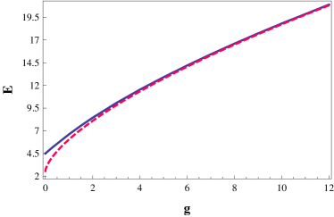
Figure 1: Comparison of the approximations (12) (broken curve) with the numerically exact results (continuous curve).

However, the results of Fig. 1 are not a good indicator of the accuracy of the approximate bosonic wavefunctions (13). To gain insight into their range of applicability, we analyse their ability to reproduce the numerically exact bechaviour of the degree of correlation degree

$$K=[tr\hat{\rho}^{2}]^{-1}=[\int\rho(x,y)^{2}dxdy]^{-1},$$ (17)

where $\rho$ is the RDM expressed in coordinates

$$\rho(x,y)=\int\psi(x,x_{2},x_{3})\psi(y,x_{2},x_{3})dx_{2}dx_{3}.$$ (18)

The degree of correlation $K$ counts approximately the number of orbitals actively involved in the Schmidt decomposition of the RDM and is one of the transparent measures of correlation. It is worth stressing at this point that the linear correlation entropy $L$, which is also a popular measure of correlation manz ; lin3 ; monk ; kosPLA ; helium , is related to $K$ via $L=1-1/K$. The results for the degree of correlation calculated from the numerically exact bosonic wavefunctions and the approximate ones $\psi_{B}^{ap}$ (13) are plotted in Fig. 2 up to $g=200$.

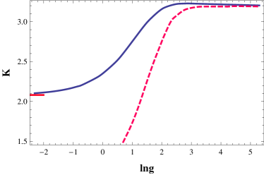
Figure 2: Degree of correlations calculated from the numerically exact wavefunctions (continuous curve) and the approximate ones (13) (broken curve), as a function of $\ln g$. The horizonal line marks the result determined as $g\rightarrow 0$ with the use of (16).

As one can see, acceptable results are reached just at a value of about $g=200$ ($\ln 200\approx 5.29$). To complete our discussion, we compare the densities $n(x)=3\rho(x,x)$ evaluated from the approximate bosonic wavefunctions (13) with the exact ones determined numerically.

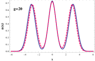
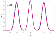
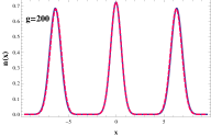
Figure 3: Comparison of one-particle density $n(x)=3\rho(x,x)$ calculated from the approximate bosonic wavefunction (13) (broken curve) with the exact one determined numerically (continuous curve), for $g=20$ $(\ln 20\approx 3)$, $g=50$ $(\ln 50\approx 3.9)$, and $g=200$ $(\ln 200=5.29)$.

Our results are displayed in Fig. 3, for three different values of the interaction strength: $g=20,50$, and $g=200$. As one could have expected, the agreement between the approximate and exact densities is observed, at least within the graphical accuracy, only in the last case.

4 Asymptotic expansion of the RDM

Now we come to the main goal of this paper, which is to provide the Schmidt decomposition of the RDM in the strong-correlation limit. To begin with our analysis, we take into consideration the RDM for the approximate wavefunction $\psi_{B}^{ap}$ (13),

$$\rho_{ap}(x,y)=\int\psi_{B}^{ap}(x,x_{2},x_{3})\psi_{B}^{ap}(y,x_{2},x_{3})dx_{2}dx_{3}$$ (19)

which becomes exact as $g\rightarrow\infty$ ($x_{c}\rightarrow\infty$). An easy inspection of Eq. (19) reveals that in this limit, it reduces to the form

$$\rho_{ap}^{g\rightarrow\infty}=\rho^{g\rightarrow\infty}=\rho_{1}+\rho_{2}+\rho_{3},$$ (20)

with

$$\rho_{1}(x,y)=A\int\psi_{ap}(z_{1},x,z_{2})\psi_{ap}(z_{1},y,z_{2})dz_{1}dz_{2},$$ (21)

$$\rho_{2}(x,y)=$$

$$=A\int\psi_{ap}(x+x_{c},z_{1},z_{2})\psi_{ap}(y+x_{c},z_{1},z_{2})dz_{1}dz_{2},$$ (22)

and

$$\rho_{3}(x,y)=$$

$$=A\int\psi_{ap}(z_{1},z_{2},x-x_{c})\psi_{ap}(z_{1},z_{2},y-x_{c})dz_{1}dz_{2},$$ (23)

where $A=2C_{\infty}^{2}$. We have obtained exact closed-form solutions for the above integrals. However, since they are quite lengthy, we report here only their numerical expressions

$$\rho_{1}(x,y)\approx 0.2407e^{-0.8944x^{2}+0.1499xy-0.8944y^{2}}.$$ (24)

$$\rho_{2/3}(x,y)\approx$$

$$\approx 0.2262e^{-0.7618[(x\pm x_{c})^{2}+(y\pm x_{c})^{2}]+0.0770(x\pm x_{c})(y\pm x_{c})},$$ (25)

which does not limit the generality of our further consideration. It it worthwhile to note here that the same asymptotic behaviour for the RDM will be obtained for the case of fermions.

Using Eq. (20), we can obtain a closed-form asymptotic expression for the one-particle density:

$$n^{g\rightarrow\infty}=3\rho^{g\rightarrow\infty}(x,x)\approx 3(0.2407e^{-1.6389x^{2}}+$$

$$+0.2262e^{-1.4466(x-x_{c})^{2}}+0.2262e^{-1.4466(x+x_{c})^{2}}).$$ (26)

An inspection of the computed $n^{g\rightarrow\infty}$ shows that it exhibits exactly the Gaussian peaks centred at the classical equilibrium positions of the particles. It is worth emphasizing that the peaks at $x=\pm x_{c}$ have the same profile.

Being real and symmetric, the function $\rho_{1}$ (24) has the Schmidt decomposition

$$\rho_{1}(x,y)=\sum_{l=0}\lambda_{l}^{(1)}u_{l}(x)u_{l}(y),$$ (27)

where $\{u_{l}\}$ and $\{\lambda_{l}^{(1)}\}$ are determined by

$$\int\rho_{1}(x,y)u_{l}(y)dy=\lambda_{l}^{(1)}u_{l}(x),$$ (28)

$\langle u_{l}|u_{k}\rangle=\delta_{lk}$. One can note that the introduction of new coordinates in the functions $\rho_{2}$ (25) and $\rho_{3}$ (25) by

$$x\mapsto\tilde{x}-x_{c},y\mapsto\tilde{y}-x_{c},$$ (29)

and

$$x\mapsto\tilde{x}+x_{c},y\mapsto\tilde{y}+x_{c},$$ (30)

respectively, transforms them into $g$-independent forms which are identical to each other, $\rho_{2}(x,y),\rho_{3}(x,y)\mapsto\tilde{\rho}(\tilde{x},\tilde{y})$,

$$\tilde{\rho}(\tilde{x},\tilde{y})\approx 0.2262e^{-0.7618(\tilde{x}^{2}+\tilde{y}^{2})+0.0770\tilde{x}\tilde{y}}.$$ (31)

The above function is also real and symmetric, thus its Schmidt decomposition is

$$\tilde{\rho}(\tilde{x},\tilde{y})=\sum_{l=0}\lambda_{l}^{(2)}v_{l}(\tilde{x})v_{l}(\tilde{y}),$$ (32)

where $\{v_{l}\}$ and $\{\lambda_{l}^{(2)}\}$ are determined by

$$\int\tilde{\rho}(\tilde{x},\tilde{y})v_{l}(\tilde{y})d\tilde{y}=\lambda_{l}^{(2)}v_{l}(\tilde{x}),$$ (33)

$\langle v_{l}|v_{k}\rangle=\delta_{lk}$. By changing the variables back in (32) in accordance with (29), one gets the expansion of $\rho_{2}$ in the form

$$\rho_{2}(x,y)=\sum_{l=0}\lambda_{l}^{(2)}v_{l}(x+x_{c})v_{l}(y+x_{c}).$$ (34)

On the other hand, the change of variables back in (32) in accordance with (30), yields the expansion of $\rho_{3}$ as

$$\rho_{3}(x,y)=\sum_{l=0}\lambda_{l}^{(2)}v_{l}(x-x_{c})v_{l}(y-x_{c}).$$ (35)

Obviously, the one-particle orbitals $v_{l}(x\pm x_{c})$ satisfy $\langle v_{l}(x\pm x_{c})|v_{k}(x\pm x_{c})\rangle=\delta_{lk}$. Finally, substitution of Eqs. (27), (34), and (35) into (20) gives, as $g\rightarrow\infty$ ($x_{c}\rightarrow\infty$),

$$\rho^{g\rightarrow\infty}=$$

$$=\sum_{l=0}[\lambda_{l}^{(1)}u_{l}(x)u_{l}(y)+\lambda_{l}^{(2)}v_{l}(x+x_{c})v_{l}(y+x_{c})+$$

$$+\lambda_{l}^{(2)}v_{l}(x-x_{c})v_{l}(y-x_{c})].$$ (36)

In this limit, the family $\{u_{l}(x),v_{l}(x-x_{c}),v_{l}(x+x_{c})\}$ forms a complete and orthonormal set, since the integral overlaps $\langle v_{l}(x+x_{c})|v_{k}(x-x_{c})\rangle$, $\langle u_{l}(x)|v_{k}(x-x_{c})\rangle$ and $\langle u_{l}(x)|v_{k}(x+x_{c})\rangle$ vanish for any $l,k$. We can therefore recognize Eq. (36) as the Schmidt decomposition of the asymptotic RDM $\rho^{g\rightarrow\infty}$. Because the asymptotic natural orbitals $v_{l}(x+x_{c})$ and $v_{l}(x-x_{c})$ correspond to the same occupancy $\lambda_{l}^{(2)}$, i.e., double degeneracies in the spectrum of the RDM $\rho^{g\rightarrow\infty}$ occur, the Schmidt decomposition (36) fails to be unique Ghirardi . Before going further we stress that the conservation of probability for the asymptotic occupancies gives $\sum_{l=0}[\lambda_{l}^{(1)}+2\lambda_{l}^{(2)}]=1$. For the sake of completeness, we give below another form of the Schmidt expansion of $\rho^{g\rightarrow\infty}$, different from that of Eq. (36). To begin with, we extend the results of Ghirardi to the case of more than one point of double degeneracy. From the orbitals $v_{l}(z+x_{c})$ and $v_{l}(z-x_{c})$, which correspond to $\lambda_{l}^{(2)}$, we define the new orbitals to be

$$\eta_{l}(z)={v_{l}(z+x_{c})+v_{l}(z-x_{c})\over\sqrt{2}},$$ (37)

and

$$\tau_{l}(z)={v_{l}(z+x_{c})-v_{l}(z-x_{c})\over\sqrt{2}},$$ (38)

that fulfill $\langle\eta_{l}|\tau_{l}\rangle=0$. In terms of them, Eq. (36) can be rewritten as

$$\rho^{g\rightarrow\infty}=\sum_{l=0}[\lambda_{l}^{(1)}u_{l}(x)u_{l}(y)+\lambda_{l}^{(2)}\eta_{l}(x)\eta_{l}(y)+$$

$$+\lambda_{l}^{(2)}\tau_{l}(x)\tau_{l}(y)],$$ (39)

Since in the limit as $g\rightarrow\infty$ ($x_{c}\rightarrow\infty$) we have $\langle\eta_{l}|\eta_{k}\rangle=\delta_{lk}$, $\langle\tau_{l}|\tau_{k}\rangle=\delta_{lk}$ and the integral overlaps $\langle u_{l}|\eta_{k}\rangle$, $\langle u_{l}|\tau_{k}\rangle$, $\langle\eta_{l}|\tau_{k}\rangle$ vanish for any $l,k$, Eq. (39) yields nothing other than a Schmidt form different from Eq. (36).

The integral equations (28) and (33) can easily be solved through a discretization technique (see for example kosPLA ). The two lowest asymptotic occupancies are found numerically to be $\lambda_{0}^{(1)}\approx 0.3193,\lambda_{0}^{(2)}\approx 0.3249$. Because the sum of all the remaining asymptotic occupancies,
$\sum_{l=1}[\lambda_{l}^{(1)}+2\lambda_{l}^{(2)}]$, is only about $0.03$, it follows that in (36) and in (39) only the terms with $l=0$ are important and, in consequence, $\rho^{g\rightarrow\infty}$ approaches the form

$$\rho^{g\rightarrow\infty}\approx$$

$$\approx\lambda_{0}^{(1)}u_{0}(x)u_{0}(y)+\lambda_{0}^{(2)}v_{0}(x+x_{c})v_{0}(y+x_{c})+$$

$$+\lambda_{0}^{(2)}v_{0}(x-x_{c})v_{0}(y-x_{c}),$$ (40)

in particular.

We close our discussion with Fig. 4, which shows the numerically determined behaviour of $\lambda_{l}$, for $l=0-2$ as a function of $\ln g$. It is seen how the occupancies converge to their asymptotic values determined by the integral equations (28) and (33), which confirms their validity. In particular, we observe how $\lambda_{0}$ and $\lambda_{1}$ converge to an asymptotic doublet.

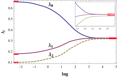
Figure 4: The dependence of the three lowest occupancies on $\ln g$. The inset highlights their changes for large values of $g$. The asymptotic values are marked by horizontal lines. The values of asymptotic occupancies $\lambda_{0}^{(2)}=\lambda_{0}^{g\rightarrow\infty}=\lambda_{1}^{g\rightarrow\infty},\lambda_{0}^{(1)}=\lambda_{2}^{g\rightarrow\infty}$ are reported in the text, whereas, the values of three lowest occupancies determined as $g\rightarrow 0$ with the use of (16) are found numerically to be $\lambda_{0}^{g\rightarrow 0}\approx 0.6619$, $\lambda_{1}^{g\rightarrow 0}\approx 0.1755$, $\lambda_{2}^{g\rightarrow 0}\approx 0.1004$.

5 Summary

In conclusion, we investigated the ground-state correlation properties of the system composed of three charged bosons in a 1D harmonic trap. Using the harmonic approximation we explained the nature of the degeneracies appearing as $g\rightarrow\infty$ in the spectrum of the RDM. An explicit representation of the asymptotic natural orbitals and their occupancies has been derived in terms of some $g$-independent integral equations. Among other results, we found that in the $g\rightarrow\infty$ limit the occupancies $\lambda_{0}^{(2)}=\lambda_{0}^{g\rightarrow\infty}=\lambda_{1}^{g\rightarrow\infty}\approx 0.3249$, $\lambda_{0}^{(1)}=\lambda_{2}^{g\rightarrow\infty}\approx 0.3193$ are the only three that have considerable values. In other words, it turned out that only the three natural orbitals contribute significantly to the asymptotic bosonic ground-state. We also determined numerically the three lowest occupancies as functions of $g$ and showed how they tend to their asymptotic values. In particular, we obtained a closed-form asymptotic expression for the one-particle density given as a linear combination of Gaussian functions centred at the classical equilibrium positions of the particles.

It would be interesting to fully investigate the effect of the number of particles on the correlation properties in 1D systems of strongly interacting bosons and/or spin fermions with a Coulomb interaction. To the best of our knowledge, there is still a lack of studies along this line. We hope our results will stimulate others to undertake the investigation of this issue. This will be also a subject of our further research.

References

- (1) N. Nielsen and I. Chuang, Quantum Computation and Quantum Information (Cambridge: Cambridge University Press), 2000.
- (2) A. Harju, S. Siljamäki, and R. M. Nieminen, Phys. Rev. B 65 075309 (2002).
- (3) A. Puente, L. Serra, and R. Nazmitindov, Phys. Rev. B 69, 125315 (2004).
- (4) N. Simonović and R. Nazmitindov, Phys. Rev. B 67, 041305 (2003).
- (5) O. Ciftja and M. G. Faruk, J. Phys.: Condens. Matter 18, 2623 (2006).
- (6) D. Manzano, et al., J. Phys. A: Math. Theor. 43, 275301 (2010).
- (7) R. Yañez, A. Plastino, and J. Dehesa, Eur. Phys. J. D 56, 141 (2010).
- (8) P. A. Bouvrie, et al., Eur. Phys. J. D 66, 15 (2012)
- (9) H. Laguna and R. Sagar, J. Phys. A: Math. Theor. 45, 025307 (2012).
- (10) H. Laguna and R. Sagar, Phys. Rev. A 84, 012502 (2011).
- (11) P. Kościk and A. Okopińska, Phys. Lett. A 374, 3841 (2010).
- (12) P. Kościk, Phys. Lett. A 375, 458 (2011).
- (13) P. Kościk and A. Okopińska, J. Phys. A: Math. Theor. 40, 1045 (2007).
- (14) P. Kościk and A. Okopińska, arXiv:1201.5504.
- (15) B. Sun and M. Pindzola, Phys. Lett. A 373, 3833 (2009).
- (16) J. Wang, C. K. Law, and M. C. Chu, Phys. Rev. A 72, 022346 (2005).
- (17) S. Zöllner, H. Meyer, and P. Schmelcher, Phys. Rev. A 74, 053612 (2006).
- (18) S. Zöllner, H. Meyer, and P. Schmelcher, Phys. Rev. A 74, 063611 (2006).
- (19) M. D. Girardeau, E. M. Wright, and J. M. Triscari, Phys. Rev. A 63, 033601 (2001).
- (20) B. Sun, D. Zhou, and L. You, Phys. Rev. A 73, 012336 (2006).
- (21) M. Girardeau, J. Math. Phys. (N.Y.) 1 , 516 (1960)
- (22) Y. He and C. Bao, J. Phys. B: At. Mol. Opt. Phys. 34, 1641 (2001).
- (23) T. Schneider and R. Blümel, J. Phys. B: At. Mol. Opt. Phys. 32, 5017 (1999).
- (24) Y. Kim and A. Zubarev, Phys. Rev. A 64, 013603 (2001).
- (25) A. Gonzalez,et al., Phys. Rev. B 59, 1653 (1999).
- (26) G. Morigi and H. Walther, Eur. Phys. J. D 13, 261, (2001)
- (27) G. E. Astrakharchik and M. D. Girardeau, Phys. Rev. B 83, 153303 (2011).
- (28) J. Ciosłowski and K. Pernal, J. Chem. Phys. 125, 064106 (2006).
- (29) J. Wineland, et al., Phys. Rev. Lett. 59, 2935 (1987).
- (30) R. Grobe, K. Rza̧żewski, and J. H. Eberly, J. Phys. B 27, L503 (1994).
- (31) G. Ghirardi and L. Marinatto, Phys. Rev. A 70, 012109 (2004).
- (32) J. S. Dehesa, et al., J. Phys. B: At. Mol. Opt. Phys. 45, 015504 (2012).