Self-exciting hurdle models for terrorist activity

Abstract

A predictive model of terrorist activity is developed by examining the daily number of terrorist attacks in Indonesia from 1994 through 2007. The dynamic model employs a shot noise process to explain the self-exciting nature of the terrorist activities. This estimates the probability of future attacks as a function of the times since the past attacks. In addition, the excess of nonattack days coupled with the presence of multiple coordinated attacks on the same day compelled the use of hurdle models to jointly model the probability of an attack day and corresponding number of attacks. A power law distribution with a shot noise driven parameter best modeled the number of attacks on an attack day. Interpretation of the model parameters is discussed and predictive performance of the models is evaluated.

and

1 Introduction

Since the attacks of September 11, 2001 there has been a substantial increase in the amount of resources dedicated to combating terrorism. As a single example, the Congressional Research Services estimates that as of September 2010 $1.2 trillion USD has been spent on the Global War on Terror, including $28.5 billion USD on enhanced security [Belasco (2010)]. Despite this increase in spending, there are no accurate measures of the effectiveness of these counter-terrorism efforts [Lum, Kennedy and Sherley (2006), Perl (2007)]. According to the Congressional Research Service, one of the keys to combating terrorism effectively is to understand, and have correctly specified models for, terrorist activity:

“Better understanding of the dynamics of terrorism allows for a more complete picture of the complexities involved in measuring success or failure and can assist the 110th Congress as it coordinates, funds, and oversees anti-terrorism policy and programs” [Perl (2007)].

A dynamic model for terrorism should describe terrorist activity in a way that is consistent with both the theoretical framework for terrorism and the observed data. Defining accurate models of terrorist activity is important not just from the standpoint of assessing the effectiveness of counter-terrorism efforts but also for use as a tool to predict the future risk of terrorist attack.

A majority of publications in the literature use one of three basic modeling approaches to terrorism. The work of Enders and Sandler (1993, 2000, 2002, 2006) and Barros (2003) uses time series analysis techniques including intervention analysis and vector autoregressive (VAR) models. Other more recent papers have applied group based trajectory analysis [Nagin (2005)] to analyze terrorist data. Examples of this include LaFree, Morris and Dugan (2010) who incorporate a zero-inflated Poisson distribution to account for an excess of zero counts. Other approaches use Cox proportional hazards models to directly model the time between attacks [Dugan, LaFree and Piquero (2005), LaFree, Dugan and Korte (2009)]. These last two papers attempt to account for the recent event history as influencing current events by constructing an ad hoc term that describes the recent density of attacks. While this is a step toward incorporating the dynamics related to the process history, it requires prespecification of the form of dependence.

The desire to include terms to account for recent event history is rooted in the theoretical understanding of terrorism and other politically motivated violence. The clustering hypothesis, concurrent with contagion theory [Midlarsky (1978)], explains politically motivated violent activity as a series of nonindependent events, where each event influences the probability of subsequent events. This hypothesis is well accepted in criminological and sociological approaches to terrorism. Clustering effects and contagious behavior have been demonstrated in military coups [Li and Thompson (1975)], international terrorism [Midlarsky, Crenshaw and Yoshida (1980)], airline hijackings [Holden (1986)], race riots [Myers (2000)] and insurgent activity [Townsley, Johnson and Ratcliffe (2008)].

In examining terrorism data in general there are two major issues to address. The first is that as terrorist attacks are usually rare, the daily number of terrorist attacks are often zero, but due to large coordinated attacks there are some extreme values. This combination of a large number of zeros and extreme values is poorly modeled by standard probability distributions. Second, the timing of terrorist incidents appear to be clustered, rendering standard models that assume independence unsuitable.

The first of these issues is addressed using a hurdle model [Mullahy (1986)], also known as the two-part model [Heilbron (1994)]. The hurdle model is a two component model that allows separate specifications of the probability of a zero count and the probability of a nonzero count. This allows the hurdle model to accommodate a large number of zeros in addition to some extreme counts. The hurdle model is used in a variety of applications, including in ecology for modeling counts of rare species [Welsh et al. (1996)], in public health for modeling smoking behavior [Jones (1994)], in political science for modeling proportional representation in minority electorates [Marschall, Ruhil and Shah (2010)] and network change detection [Heard et al. (2010)]. For terrorism modeling, the hurdle model is preferred to the zero-inflated model [Lambert (1992)] which assumes that the extra zeros observed are due to censoring. The hurdle model assumes that the extra zeros are due to a separate process (the “hurdle”), which must be overcome before the number of corresponding incidents are determined. This is more reasonable for terrorism data, as it can often be assumed that sparsity of attacks is because they are indeed rare, not because they are unobserved.

The second issue regarding the clustering behavior of terrorist activity is addressed by incorporating a self-exciting component [Hawkes (1971)]. The self-exciting component specifies that the probability of a event is a function of the time (and possibly other aspects) of all previous events, such that the effect on the probability decreases over time. This can help account for the clustering and dynamic nature of terrorism. For example, Holden (1986, 1987) developed a self-exciting Poisson model that better represented the dynamics of airline hijacking and Mohler et al. (2011) a self-exciting space–time model for residential burglaries.

This paper combines these two concepts to examine the use of self-exciting hurdle models for terrorist activity in Indonesia and Timor-Leste between 1994 and 2007. The hurdle component is modeled as a self-exciting Bernoulli process where the form of self-excitation is dictated by the data. The nonzero counts are modeled by an extreme value distribution with parameters that are also a function of the event history. The corresponding self-exciting hurdle model is capable of making predictions and providing information about the risk of terrorist activity without any additional covariate information other than the event history. This capability is important as covariate information for terrorism data is often either missing or unreliable.

2 Data and exploratory analysis

The Global Terrorism Database [LaFree and Dugan (2007)] is an open-source publicly available database of over 87,000 terrorist events around the world from 1970 through 2008. The database is continually updated with new information and is believed to be the most comprehensive database of its kind. The data used here are a subset of the GTD consisting of daily counts of terrorist attacks in Indonesia from January 1, 1994 through December 31, 2007.

2.1 Exploratory data analysis

The data from a training period of 1994 through 2000 was examined to inform model construction. Of the 2,557 days considered in this analysis, there were 250 terrorist attacks on 158 unique event days. Figure 1, displaying the daily and semi-yearly counts of attacks, illustrates the nature of the terrorist activity. In particular, the attacks appear clustered with long stretches between attacks followed by a period of increased activity. In addition, while most days have no attacks (93.8%), some days have multiple attacks (possibly due to planned coordinated attacks).

Table 1: Distribution of observed and expected number of Indonesian terrorist attacks per day (1994–2000)

# Attacks	# Days	Poisson	Neg.Bin
0	$2\mbox{,}399$	$2\mbox{,}319$	$2\mbox{,}401$
1	$130$	$227$	$103$
2	$16$	$11$	$31$
3	$7$	$0$	$12$
4	$1$	$0$	$5$
$>$4	$4$	$0$	$5$
AIC	–	$1\mbox{,}988.0$	$1\mbox{,}481.8$

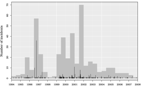
Figure 1: Daily number of terrorist events in Indonesia. The histogram shows the cumulative number of attacks in each six month period.

Table 1 shows the distribution of the observed attacks per day compared to the expected values under a Poisson and negative binomial probability distribution fitted with maximum likelihood. While the Poisson cannot capture any of the tail behavior, the negative binomial adapts better to the tail distribution but consequently underestimates the number of days with only 1 attack and overestimates the number of days with 2 and 3 attacks. A chi-square goodness-of-fit test yields a $p$-value of $0.00016$, suggesting that the negative binomial is not a sufficient model. In addition, the tail is comprised of several extreme values ($36,11,10$ and 6 attacks on a single day) that exacerbate the general lack of fit. The large number of zeros coupled with the presence of several extreme values necessitate more complex models.

Figure 1 also reveals the possibility that the attack days are clustered. This is examined with Ripley’s $K$-function [Dixon (2002)]. The $K$-function is a second-order function that can reveal if clustering (or inhibition) is present in a point pattern. It is defined loosely as

$$K(t)\propto\mathbb{E}[\mbox{\# of future events $\leq t$ from a randomly chosen event}].$$

Because this measure will be effected by an inhomogeneous attack day probability, we estimate it [Baddeley, Møller and Waagepetersen (2000), Veen and Schoenberg (2006)]:

$$\hat{K}(t)=T^{-1}\sum_{i=1}^{N}\frac{w_{i}}{\hat{p}_{i}}\sum_{j>i}\frac{\mathbh{1}(t_{j}-t_{i}\leq t)}{\hat{p}_{j}},$$

where $T$ is the total observational time, $\hat{p}_{i}$ is the estimated probability of at least one attack at day $t_{i}$, and $w_{i}$ is a one-sided edge correction. The estimated probability is given by the model in (9) that includes trend and seasonality components (i.e., model BL₅ in Table 2; see Section 4).

Figure 2 plots $\hat{K}(t)-t$ which has expected value 0 if the estimated probabilities are correct and there is no unaccounted for clustering. The observed values fall well above the 95% pointwise confidence intervals (obtained from a parametric bootstrap, 1,000 simulations), showing that the data display clustering behavior not accounted for by the baseline model.

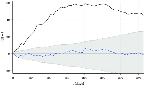
Figure 2: Plot of $\hat{K}(t)-t$ for Indonesian terrorism (1994–2000). The solid line is from the baseline model (BL₅) with the gray band showing the 0.025 and 0.975 quantiles estimated from 1,000 simulations. The dashed line is from the self-exciting model (SE₁) presented in Section 4.

These characteristics of the terrorism data require flexible models that can handle the temporal attack patterns, clustering, an excess of nonattack days and the possibility of multiple coordinated attacks on the same day. Self-exciting hurdle models are developed in the next section to represent the complex nature of such terrorist activity.

3 Hurdle models and the self-exciting process

3.1 Hurdle models

The hurdle models of Mullahy (1986) refer to a class of two component models for discrete count data. These models assume that two different processes drive the zero and nonzero counts, respectively. The hurdle component of the model corresponds to the probability that the count is nonzero (i.e., a terrorist action will occur), while the count component corresponds to the distribution of positive counts (i.e., the number of corresponding terrorist events). When the two components are combined, the hurdle model produces a probability mass function on the nonnegative integers. Additionally, the hurdle approach facilitates the use of two simpler models in place of one more complicated model. This will be especially appealing in model fitting, as the likelihood may be separable, allowing for independent evaluation of each component.

For modeling the daily counts of a terrorist process, let $Y_{t}$ be the number of events on day $t$ and $E_{t}$ be the indicator for an event day such that $E_{t}=1$ if $Y_{t}\geq 1$ (i.e., there is at least one terrorist attack on day $t$) and $E_{t}=0$ if $Y_{t}=0$ (i.e., there are no attacks on day $t$). Also, let $t_{i}$ denote the $i$th event day (not event, but day with at least one attack).

Letting $\mathcal{H}_{t}=\{Y_{s}\dvtx s\leq t\}$ be the internal history of the terrorist process, the hurdle component is modeled as a Bernoulli random variable with hurdle probability $p_{t}=\Pr(E_{t}=1|\mathcal{H}_{t-1})$ specified conditionally on the past history of the event process. A separate count model is constructed for $Y_{t}|E_{t}=1$ with density $f_{t}(y)=\Pr(Y_{t}=y|E_{t}=1,\mathcal{H}_{t-1})$, for $y\in\{1,2,\ldots\}$. Because the count component is constructed conditionally on there being at least one event, it will have no support on 0 [i.e., $f_{t}(0)=0$]. Combining the hurdle and count components gives the full density

$$f^{*}_{t}(y)=\Pr(Y_{t}=y|\mathcal{H}_{t-1})=\cases{f_{t}(y)p_{t},&\quad$y>0$,\cr 1-p_{t},&\quad$y=0$.}$$ (1)

This has a similar form to a zero-inflated model [Lambert (1992)] but differs in that for the zero-inflated model $\Pr(Y_{t}=0|\mathcal{H}_{t-1})=(1-p_{t})f_{t}(0)$. Zero-inflated models usually arise when there is a random censoring process that prevents observations at certain times. Alternatively, instead of assuming that terrorist events occurred but were not observed, the hurdle approach explicitly models the probability that no events occurred.

The log-likelihood for a hurdle model can be decomposed as the sum of two terms $\log L=\log L_{1}+\log L_{2}$, where for $T$ observations

$$\log L_{1} = \sum_{t=1}^{T}E_{t}\log p_{t}+(1-E_{t})\log(1-p_{t}),$$ (2)

$$\log L_{2} = \sum_{t=1}^{T}E_{t}\cdot\log f_{t}(y_{t})$$

$$= \sum_{t\dvtx E_{t}=1}\log f_{t}(y_{t}).$$

The first term (in the form of a Bernoulli process) represents the hurdle component and the second term is the usual sum for a set of observations coming from the density $f_{t}$ and represents the number of events per event day. The form of the likelihood is equivalent to a discrete time version of a marked point process [Daley and Vere-Jones (2003)], where the marks are the number of attacks on an event day. A particular benefit of this representation emerges when $f_{t}$ and $p_{t}$ share no common parameters, allowing their log-likelihoods to be handled separately for parameter estimation.

3.2 Self-exciting process

It has been suggested that some terrorist processes exhibit self-excitation or contagion behavior [Holden (1986), Dugan, LaFree and Piquero (2005), LaFree, Dugan and Korte (2009)]. A self-exciting point process [Hawkes (1971)] is one where the realization of events increases the short-term probability of observing future events, much in the same manner that one contagious individual can infect other individuals (while they are still infectious) or how major earthquakes lead to aftershocks. This type of model can be written in the form of a cluster process [Hawkes and Oakes (1974)] and used to explain the apparent clustering of terrorist activities. Specifically, we consider a generalized shot noise process [Rice (1977)], where the self-exciting component $S_{t}\geq 0$ will be a nonnegative function of the past history $\mathcal{H}_{t-1}$ of the form

$$S_{t} = \sum_{s<t}E_{s}\alpha_{s}g(t-s)$$

$$= \sum_{i\dvtx t_{i}<t}\alpha_{i}g(t-t_{i}).$$

The magnitude parameter, $\alpha_{i}$, determines the influence that the $i$th event day has on the self-exciting process. It may be a function of other associated information about the event day (e.g., number of events, number killed, success indicator, group attribution). Based on the results of the exploratory data analysis, we restrict our attention to the case where $\alpha_{i}\geq 0$, although inhibition effects could be obtained if negative values were permitted.

The decay function $g(\cdot)$ specifies the shape of the excitation based on the time since the previous event days. To aid in parameter interpretation and estimation, we specify $g(\cdot)$ to be a proper probability mass function with strictly positive support such that $g(u)\geq 0$, $g(u)=0$ for $u<1$, and $\sum_{u=1}^{\infty}g(u)=1$. This ensures that the influence of an event will eventually diminish and makes $\alpha_{i}$ solely responsible for the magnitude of the effects contributed by the $i$th event.

Any discrete distribution can be used for the decay function, provided its support is limited to the set of positive integers. Standard distributions, like Poisson or negative binomial, may require shifting or truncation to avoid having support on zero. For example, the (mean specified) shifted negative binomial is

$$g(u;\mu,r)=\frac{\Gamma(r+u-1)}{\Gamma(r)(u-1)!}\biggl{(}\frac{r}{\mu-1+r}\biggr{)}^{r}\biggl{(}\frac{\mu-1}{\mu-1+r}\biggr{)}^{u-1},$$ (5)

which has a mean of $\mu>1$, and size parameter $r>0$. The corresponding shifted geometric distribution is given by $g(u;\mu,r=1)$ and the shifted Poisson density can be defined as the limiting case when $r\rightarrow\infty$.

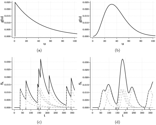
Figure 3: (a) and (b) show the decay functions for the shifted geometric ($\mu=40$) and shifted negative binomial ($\mu=40,r=5$), respectively. (c) and (d) show the corresponding shot noise processes (solid lines) and scaled component kernels (dotted lines) for 8 events with $\alpha_{i}=\alpha=0.5$.

Figure 3 shows the geometric and negative binomial decay functions along with the shot noise processes corresponding to 8 event days. This illustrates how the form of the shot noise process from (3.2) is similar to kernel intensity estimation [Diggle (1985)], but with weights and one-sided (predictive) kernels.

3.3 Self-exciting Bernoulli hurdle process

The event days, $E_{t}$, are modeled as a self-exciting Bernoulli process where the probability of an event day is excited (increased) by the occurrence of previous events. Specifically, we consider the hurdle probability on day $t$ to be a function of the process

$$X_{t}=B_{t}+S_{t},$$ (6)

where $B_{t}$ is a baseline process and $S_{t}$ is the self-exciting component given by (3.2). The baseline can be a function of any exogenous variables that could have an effect on the process (e.g., social, political or economic conditions and events, counter-terrorism efforts, etc.), but it will not include any information coming from the internal history.

To ensure the hurdle probability $p_{t}\in[0,1]$, a transformation $\eta(p_{t})=X_{t}$ is used. If the baseline process is nonnegative (i.e., $B_{t}\geq 0$), then $X_{t}\geq 0$ and an appealing transformation is $\eta(p)=-\log(1-p)$, corresponding to the hurdle probability

$$p_{t}=1-e^{-X_{t}}.$$ (7)

While other transformations (e.g., logit) could be used, this one provides several benefits. It enjoys a likelihood function that is computationally convenient, substituting (7) into (2) obtains the Bernoulli log-likelihood

$$\log L_{1}=\sum_{1\leq t_{i}\leq T}\log(e^{X_{t_{i}}}-1)-\sum_{t=1}^{T}X_{t}.$$ (8)

The shot noise component of the second sum $(\sum_{t=1}^{T}X_{t}=\sum_{t=1}^{T}B_{t}+\sum_{t=1}^{T}S_{t})$ can be simplified by recognizing that

$$\sum_{t=1}^{T}S_{t}=\sum_{i\dvtx t_{i}<T}\alpha_{i}G(T-t_{i}),$$

where $G$ is the cumulative density function of $g$. This significantly reduces computation, as it is only calculated for the event days and not over all days in the observation window.

This transformation also allows for a straightforward interpretation of the parameters in $X_{t}$. Notice that $p_{t}$ is also the probability that a Poisson random variable with rate $X_{t}$ is greater than 0. When events are rare and $X_{t}$ is small, $E_{t}$ can be modeled approximately by a Poisson distribution. According to the superposition property of the Poisson, the event days arise from two sources, the baseline process with rate $B_{t}$ and the shot noise process with rate $S_{t}$. The rate from the shot noise can be further decomposed into its elements $\alpha_{i}g(t-t_{i})$ for $\{i\dvtx t_{i}<t\}$. Thus, under the Poisson approximation, event day $i$ will generate an expected $\sum_{u=1}^{\infty}\alpha_{i}g(u)=\alpha_{i}$ number of additional event days and the decay function $g(\cdot)$ controls when the extra event days will occur. While these interpretations will not hold exactly under the Bernoulli model, they do provide an indication of how each component effects the process.

3.4 Survival functions

This formulation for the hurdle process also provides simple expressions for some properties of the time until the next event day. For a given time $t_{0}$, let $\tau$ be the time of the next event day. The survival function $V_{t_{0}}(u)=\Pr(\tau-t_{0}>u)$ gives the probability that the next event day will be more than $u$ days away. For the self-exciting hurdle process, this becomes

$$V_{t_{0}}(u) = \Pr(E_{t_{0}+1}=E_{t_{0}+2}=\cdots=E_{t_{0}+u}=0)$$

$$= \prod_{\delta=1}^{u}(1-p_{t_{0}+\delta})$$

$$= \exp\Biggl{\{}-\sum_{\delta=1}^{u}X_{t_{0}+\delta}\Biggr{\}}$$

for $u\in\{1,2,\ldots\}$, where $X_{t_{0}+\delta}$ is calculated assuming no new events have occurred since $t_{0}$. The survival function can be used to calculate the expected time until the next event day

$$\mathbb{E}_{t_{0}}[\tau] = \mathbb{E}[\tau-t_{0}]=1+\sum_{u=1}^{\infty}V_{t_{0}}(u)$$

$$= 1+\sum_{u=1}^{\infty}\exp\Biggl{\{}-\sum_{\delta=1}^{u}X_{t_{0}+\delta}\Biggr{\}}.$$

The survival function specification of this model can be useful for prediction, and making inference about future attacks given the current history.

4 Results

In order to build the models and evaluate their predictive performance, the data are partitioned into two time periods. The first time period from 1994 through 2000 is used to construct the models and estimate their parameters. The second period from 2001 through 2007 is used to assess the predictive performance of the models.

4.1 Event day modeling

Recall that the hurdle probability is constructed from the sum of a baseline and self-exciting processes (6). In order to capture potential seasonality and other large scale trends in the data, the baseline process $B_{t}$ is defined as

$$\log(B_{t})=\beta_{0}+\beta_{1}t+\beta_{2}t^{2}+A_{1}\sin(2\pi t/\omega)+A_{2}\cos(2\pi t/\omega),$$ (9)

where the seasonal terms have a period of $\omega=365.25$ days. This results in five baseline parameters $\theta_{B}=(\beta_{0},\beta_{1},\beta_{2},A_{1},A_{2})\in\mathbb{R}^{5}$. The log transform ensures $B_{t}\geq 0$. We considered self-exciting processes of the form

$$S_{t}(\alpha,\mu,r)=\alpha\sum_{i\dvtx t_{i}<t}g(t-t_{i};\mu,r),$$ (10)

where $g(u;\mu,r)$ is a shifted negative binomial decay function (5) and the magnitude $\alpha$ is a constant. This results in three parameters for the self-exciting component $\theta_{S}=(\alpha,\mu,r)\in\mathbb{R}_{+}^{3}$.

The combined model for $X_{t}=B_{t}+S_{t}$ results in up to 8 parameters to estimate. Estimation is carried out by maximizing the log-likelihood function given in (8). Since there is no explicit solution available, we used R’s numerical optimization routine nlminb [R Development Core Team (2011)] to obtain estimates. For all models, the estimates converged within seconds from a variety of starting points.

Table 2: Parameter estimates for the event day models for the training period (1994–2000). The BL are the baseline only and the SE are the self-exciting models

Model	AIC	$\bolds{\beta_{0}}$	$\bolds{\beta_{1}}$	$\bolds{\beta_{2}}$	$\bolds{A_{1}}$	$\bolds{A_{2}}$	$\bolds{\alpha}$	$\bolds{\mu}$	$\bolds{r}$
BL1	1,187.77	$-2.75$
BL2	1,149.54	$-8.2$	$8.05$
BL3	1,151.25	$-2.83$	$-8.01$	$11.91$
BL4	1,171.22	$-2.82$			$-0.42$	$-0.31$
BL5	1,136.80	$-8.02$	$7.69$		$-0.35$	$-0.32$
BL6	1,138.60	$-3.53$	$-5.74$	$9.95$	$-0.35$	$-0.32$
SE1	1,075.21	$\bolds{-}$4.41					0.89	37.54	0.45
SE2	1,077.16	$-5.17$	$1.23$				0.87	36.55	0.45
SE3	1,078.71	$15.31$	$-63.2$	$50.24$			0.85	35.69	0.45
SE4	1,077.03	$-4.34$			$-0.41$	$-0.40$	0.86	38.55	0.44
SE5	1,078.76	$-5.99$	$2.68$		$-0.38$	$-0.42$	0.82	36.57	0.43
SE6	1,079.60	$20.46$	$-79.33$	$62.91$	$-0.43$	$-0.45$	0.80	37.28	0.43

Table 2 shows the evaluated models and their corresponding AIC scores. The lowest AIC belongs to the four component model with a constant baseline (SE₁), providing essentially a discrete time version of the Hawkes model [Hawkes (1971), Ozaki (1979)]. This AIC is much lower than the best baseline only model (BL₅) which includes the periodic terms. Figure 2 plots the weighted $K$-function for SE₁ and BL₅ showing the self-exciting model is much tighter around 0 indicating a better fit over the baseline only model [Diggle (1979)]. Figure 4 shows the estimated hurdle probability in the training period for both models.

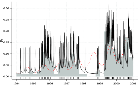
Figure 4: Hurdle probabilities for the best fitting self-exciting model SE₁ (solid line), the best fitting baseline only model BL₅ (dotted line), and the observed piecewise constant probabilities (blocks). The rug signifies the event days.

The parameters of the self-exciting model (SE₁) suggest a baseline hurdle probability of about $0.012$ when the shot noise term drops to zero. However, according to the Poisson approximation, every event day will generate an expected $\alpha=0.89$ additional event days. The generated event day is expected to occur in $\mu=37.54$ days, but the time until occurrence has a median of only 16 days.

4.2 Count modeling

It can be obtained from Table 1 that most event days (92.4%) are comprised of only 1 or 2 attacks. However, several days (1.9%) have more than 9 attacks (with one day having 36 recorded terrorist attacks). This suggests count distributions that have an initial rapid decay, but still possess a long tail to accommodate the extreme values. One such discrete distribution is the Riemann zeta or discrete Pareto distribution. This power law distribution has recently been employed to model the severity (e.g., number killed or injured) of terrorist attacks [Clauset, Young and Gleditsch (2007)].

Using it to model the event day counts, under an i.i.d assumption, gives the probability mass function

$$f_{t}(y;s)=\frac{y^{-s}}{\zeta(s)},\qquad y\in\{1,2,\ldots\},$$

where $\zeta(s)=\sum_{x=1}^{\infty}x^{-s}$ is the Riemann zeta function and the parameter $s\in(1,\infty)$. This one parameter model is easy to estimate numerically via maximum likelihood [Goldstein, Morris and Yen (2004), Seal (1952)] by finding the $s$ that satisfies the equation $\frac{1}{n}\sum_{i=1}^{n}\log(y_{i})=-\frac{\zeta^{\prime}(s)}{\zeta(s)}$. The training period data gives rise to an estimated parameter of $\hat{s}=2.86$. The bootstrap Kolmogorov–Smirnov test of Clauset, Shalizi and Newman (2009) gives a $p$-value of $0.69$, suggesting the zeta distribution provides a suitable fit.

While the constant parameter zeta distribution appears to provide a good fit, there may be better models, especially if the distribution is allowed to vary over time. In particular, as for the hurdle component, distributions that vary over time in response to a shot noise process are considered. An additional driving process (with shot noise) was implemented for the count model, namely,

$$X^{c}_{t}(\beta^{c},\alpha^{c},\mu^{c})=\beta^{c}+\alpha^{c}\sum_{i\dvtx t_{i}<t}Y_{i}\cdot g^{c}(t-t_{i};\mu^{c}),$$

where $\beta^{c}$ is a constant baseline, $\alpha^{c}_{i}=\alpha^{c}\cdot Y_{i}$ varies in response to the number of attacks on the $i$th event day, and the decay function $g^{c}(u;\mu^{c})$ is the one parameter shifted geometric function with mean $\mu^{c}$. This results in three parameters for the count component $\theta_{C}=(\beta^{c},\alpha^{c},\mu^{c})$. Note that this is a separate process than the one specified for the hurdle component given by (9) and (10). The additional flexibility afforded by the hurdle specification allows such additional complexity to be introduced for the count component of the model.

There are two primary hypotheses about how the count distribution behaves in response to the event history. First, counts could respond in a self-exciting manner, where recent event and multi-event days increase the likelihood of further multi-event days. Alternatively, due to the depletion of resources or increased anti-terrorism measures after large attacks, counts may respond in a more self-inhibiting manner, where recent multi-event days lower the chances of multi-events day in the near future.

Table 3: Parameter estimates for the count models for the training period (1994–2000). C_z, C_se and C_si are the constant parameter, self-exciting and self-inhibiting forms, respectively, of the Riemann zeta distribution

Model	AIC	$\bolds{s}$	$\bolds{\beta}$	$\bolds{\alpha}$	$\bolds{\mu}$
Cz	241.00	2.86
Cse	240.48	$(1-e^{-X_{t}})^{-1}$	$0.375$	0.20	$2.13$
Csi	244.72	$e^{X_{t}}$	$1.00$	0.34	$55.18$

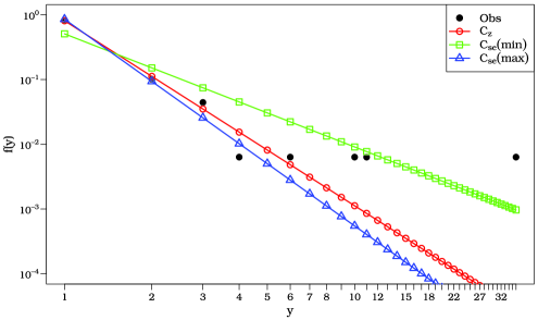
Figure 5: Estimated count probabilities for the constant parameter model (C_z with $s=2.86$) and for the self-exciting count model (C_se) at the baseline state ($s=3.19$) and most excited state ($s=1.75$).

To evaluate the self-exciting hypothesis, let $s_{t}=(1-e^{-X_{t}^{c}})^{-1}$ since smaller values of $s$ lead to more mass on the extreme values. Alternatively, $s_{t}=e^{X_{t}^{c}}$ for the self-inhibiting model. Table 3 shows the estimated parameters and AIC scores for the fitted count models. The lower AIC suggests that the self-exciting count model has more validity than the self-inhibiting model for the training data. Figure 5 shows the estimated probability of counts under the constant parameter (C_z) and self-exciting (C_se) models. While the self-exciting model puts more mass on multi-event days when $X_{t}^{c}$ is large, the decay is rapid and the self-exciting behavior is short lived—only for a few days, before the shot noise term approaches 0 and its effects become negligible.

4.3 Testing model predictions

Based on the training period, models are selected and fit for both the hurdle and count components. To evaluate how well this can predict future terrorist activity, the models are applied to the terrorist incidents in the testing period (2001–2007) using the following procedure: [(1)]

At day $t$ predict the probability of an event day and conditional number of attacks on day $t+1$, based on the current history $\mathcal{H}_{t}$.

Observe $Y_{t+1}$ and re-estimate the model parameters based on the updated history $\mathcal{H}_{t+1}$.

Repeat steps (1) and (2) through the testing period to construct a final model based on all data between 1994–2007. This update and forecast scheme results in a set of daily predictions $\hat{p}_{t}=\Pr(E_{t}=1|\mathcal{H}_{t-1})$ and $\hat{f}_{t}(y)=\Pr(Y_{t}=y|E_{t}=1,\mathcal{H}_{t-1})$ conditioned on the past history of the process.

The predictive capability of the models are evaluated by comparing the log probability gain, or predictive log-likelihood ratio, of each model [Daley and Vere-Jones (2004)]. This score is a relative measure of the improvement in predicative capability for a model compared to a reference or null model. The interpretation is that values greater than $0$ show a relative improvement in predictions over the reference model, with the highest values indicating the preferred model.

Table 4: The hurdle component log probability score, $G$, using the constant baseline only model (BL₁) as the reference model. The AIC scores are from the training period (see Table 2)

Model	AIC	$\bolds{G}$	Model	AIC	$\bolds{G}$
BL1	1,187.77	$0.00$	SE1	1,075.21	26.96
BL2	1,149.54	$-19.10$	SE2	1,077.16	25.47
BL3	1,151.25	$20.69$	SE3	1,078.71	24.96
BL4	1,171.22	$-1.39$	SE4	1,077.03	26.22
BL5	1,136.80	$-18.21$	SE5	1,078.76	24.56
BL6	1,138.60	$21.63$	SE6	1,079.60	24.57

For the hurdle component, the log probability gain is

$$G=\sum_{t\in\mathcal{T}_{2}}E_{t}\log\frac{\hat{p}_{t}}{\hat{\pi}_{t}}+(1-E_{t})\log\frac{1-\hat{p}_{t}}{1-\hat{\pi}_{t}},$$

where $\hat{p}_{t}$ comes from the model of interest and $\hat{\pi}_{t}$ from the constant baseline only model (BL₁), and $\mathcal{T}_{2}=[01$ Jan 2001, 31 Dec 2007] covers the testing period. Table 4 compares the log probability gains $G$ and the AIC scores from the training period, and shows that the results from the test period were similar to those in the training period, supporting the use of AIC for model selection.

The constant baseline self-exciting model (SE₁) has the largest log probability gain and all self-exciting models outperform all of the baseline only models. The best baseline only model for the testing period was the full model with seasonality and a quadratic trend (BL₆). This is in contrast to the training period results where the best baseline only model had a linear trend (BL₅). The linear trend model failed to perform as well during the testing period, as the general attack rate peaked around the transition point and started decreasing during the remainder of the testing period, creating a significant quadratic trend over the combined observation period. Alternatively, the self-exciting models can adapt rapidly to sudden changes in attack rate, yielding better overall predictive ability.

The count component uses the log probability gain score

$$G^{c}=\sum_{i\dvtx t_{i}\in\mathcal{T}_{2}}\log\frac{\hat{f}(y_{i})}{\hat{h}(y_{i})},$$

where $\hat{f}$ is the model of interest and $\hat{h}$ is the reference model. Table 5 shows the values of $G^{c}$ using the constant parameter zeta model (C_z) as the reference model. These results show the self-exciting zeta model (C_se) as the preferred model for predicting the counts.

=190pt C$\bolds{{}_{s}}$ C$\bolds{{}_{\mathit{se}}}$ C$\bolds{{}_{\mathit{si}}}$ $G^{c}$ 0.00 8.07 $-$0.27

Table 5: The count component log probability score, $G^{c}$, using the constant parameter zeta model (C_z) as the reference model

As with the hurdle component, the predictive performance of the count models followed the AIC scores from the training period. However, the model with the self-exciting component does predict substantially better than the constant component model—more so than would be expected from the AIC scores in the training period (see Table 3). This may be due to changes in the attack behavior during the testing period. Figure 1 shows that while there were a few large counts during 2001, there were very few multi-attack days after. This change in the pattern of multiple attacks accounts for the improved predictive capabilities of the self-exciting model over the constant parameter model. The self-exciting count model is able to quickly adapt to changing conditions and consequently makes better predictions.

In summary, the daily counts of Indonesian terrorist attacks were modeled with a self-exciting hurdle model. The separation of the model into two components allowed both the attack rate and attack characteristics to be more faithfully represented. It was found that including a self-exciting process benefited both the hurdle and count components by allowing the models to quickly adapt to changing attack behavior. It is this property as a predictive tool that makes the self-exciting hurdle model especially useful in an applied setting where prediction is of primary interest.

5 Conclusion

In practice, policy makers are faced with limited resources, financially, materially and in personnel. The allocation of these resources depends on an understanding of the future risk of terrorist activity. As an example, in the wake of the attacks of September 11, 2001, policy makers placed additional security in the form of National Guard troops in all US commercial airports. This was done in hopes of re-establishing public trust in the safety of air travel while the intelligence community was assessing the risk of subsequent attacks [Price and Forrest (2009)]. The obvious question in that case was when to shift resources from increased airport security to investing in long-term strategies to improve intelligence capabilities. As this case illustrates, only by clearly understanding the risk of terrorist activity can policy makers make informed decisions about allocating resources.

This paper presents a two-component self-exciting model for the analysis and prediction of future terrorist activity. It was found that the best model used a constant baseline with a self-exciting term for the hurdle component and a Riemann zeta distribution with shot noise driven parameter for the count component. The improvement offered by the self-exciting term provides support for the contagion theory and suggests a significant short term increase in terrorism risk after an attack. The use of a power law distribution for the number of same day attacks corresponds with the power law behavior of the number killed in terrorist attacks [Clauset, Young and Gleditsch (2007)]. This is to be expected, as multiple coordinated attacks would tend to indicate better planned, and hence more severe, terrorist activities.

The self-exciting hurdle model adheres to the theoretical concept for a contagion effect to terrorism as manifested in the clustering of data while providing good fit and predictive capabilities without relying on exogenous variables. The model provides a simple structure and interpretation of the parameters useful for understanding the dynamic nature of the terrorist activity. This provides an appropriate staring point for exploring additional covariate effects, including analysis concerning the effectiveness of counter-terrorism activities, geography, political or economical factors. As the attack clustering may be partially attributable to a stochastic baseline driven by such exogenous processes [Holden (1986)], further analysis could include covariates in the baseline model (9) to test the impact on the self-exciting component.

By focusing on the timing of terrorist attacks on the islands of Indonesia, other aspects of the attacks, such as location, attack type and group responsible, were not considered. Including such additional information could lead to more detailed models that better explain the nuances of the terrorist activity. For example, the self-exciting component could include a spatial proximity term using the models of Mohler et al. (2011) or multiple self-exciting terms could be included that represent how attacks from one terrorist group influence the subsequent attacks of other groups.

The utility of the models presented here and their ease of implementation and interpretation make them a potentially useful tool in security related fields. The results show that the risk of terrorist activity can vary greatly over short periods of time, thus policy responses in terms of resource allocation, security and counter-terrorism responses should reflect this as well as addressing the more long-term trends in risk. For example, understanding the short-term variations in risk would allow a more effective deployment and assessment of additional airport security measures in the wake of a terrorist attack, while a grasp of the longer term trends could help guide the development and assessment of more strategic counter-terrorism resources, such as increasing the number of foreign language experts available for translation or developing effective de-radicalization programs to prevent the growth of terrorist groups.

References

- Baddeley, Møller and Waagepetersen (2000) {barticle}[mr] \bauthor\bsnmBaddeley, \bfnmA. J.\binitsA. J., \bauthor\bsnmMøller, \bfnmJ.\binitsJ. and \bauthor\bsnmWaagepetersen, \bfnmR.\binitsR. (\byear2000). \btitleNon- and semi-parametric estimation of interaction in inhomogeneous point patterns. \bjournalStat. Neerl. \bvolume54 \bpages329–350. \biddoi=10.1111/1467-9574.00144, issn=0039-0402, mr=1804002 \bptokimsref \endbibitem
- Barros (2003) {barticle}[author] \bauthor\bsnmBarros, \bfnmC. P.\binitsC. P. (\byear2003). \btitleAn intervention analysis of terrorism: The Spanish ETA case. \bjournalDefence and Peace Economics \bvolume6 \bpages401–412. \bptokimsref \endbibitem
- Belasco (2010) {bmisc}[author] \bauthor\bsnmBelasco, \bfnmA.\binitsA. (\byear2010). \bhowpublishedThe cost of Iraq, Afghanistan, and other Global War on Terror Operations Since 9/11. Technical Report RL33110, Congressional Research Services. Available at http://www.fas.org/sgp/crs/natsec/RL33110.pdf. \bptokimsref \endbibitem
- Clauset, Shalizi and Newman (2009) {barticle}[mr] \bauthor\bsnmClauset, \bfnmAaron\binitsA., \bauthor\bsnmShalizi, \bfnmCosma Rohilla\binitsC. R. and \bauthor\bsnmNewman, \bfnmM. E. J.\binitsM. E. J. (\byear2009). \btitlePower-law distributions in empirical data. \bjournalSIAM Rev. \bvolume51 \bpages661–703. \biddoi=10.1137/070710111, issn=0036-1445, mr=2563829 \bptokimsref \endbibitem
- Clauset, Young and Gleditsch (2007) {barticle}[author] \bauthor\bsnmClauset, \bfnmAaron\binitsA., \bauthor\bsnmYoung, \bfnmMaxwell\binitsM. and \bauthor\bsnmGleditsch, \bfnmKristian Skrede\binitsK. S. (\byear2007). \btitleOn the frequency of severe terrorist events. \bjournalJournal of Conflict Resolution \bvolume51 \bpages58–87. \bptokimsref \endbibitem
- Daley and Vere-Jones (2003) {bbook}[author] \bauthor\bsnmDaley, \bfnmD. J.\binitsD. J. and \bauthor\bsnmVere-Jones, \bfnmD.\binitsD. (\byear2003). \btitleAn Introduction to the Theory of Point Processes. I, \bedition2nd ed. \bpublisherSpringer, \baddressNew York. \bptokimsref \endbibitem
- Daley and Vere-Jones (2004) {barticle}[mr] \bauthor\bsnmDaley, \bfnmDaryl J.\binitsD. J. and \bauthor\bsnmVere-Jones, \bfnmDavid\binitsD. (\byear2004). \btitleScoring probability forecasts for point processes: The entropy score and information gain. \bjournalJ. Appl. Probab. \bvolume41A \bpages297–312. \biddoi=10.1239/jap/1082552206, issn=0021-9002, mr=2057581 \bptokimsref \endbibitem
- Diggle (1979) {barticle}[author] \bauthor\bsnmDiggle, \bfnmPeter J.\binitsP. J. (\byear1979). \btitleOn parameter estimation and goodness-of-fit testing for spatial point patterns. \bjournalBiometrics \bvolume35 \bpages87–101. \bptokimsref \endbibitem
- Diggle (1985) {barticle}[author] \bauthor\bsnmDiggle, \bfnmPeter\binitsP. (\byear1985). \btitleA kernel method for smoothing point process data. \bjournalJ. R. Stat. Soc. Ser. C. Appl. Stat. \bvolume34 \bpages138–147. \bptokimsref \endbibitem
- Dixon (2002) {bincollection}[author] \bauthor\bsnmDixon, \bfnmP. M.\binitsP. M. (\byear2002). \btitleRipley’s K function. In \bbooktitleEncyclopedia of Econometrics (\beditor\bfnmA. H.\binitsA. H. \bsnmEl-Shaarawi and \beditor\bfnmW. W.\binitsW. W. \bsnmPiegorsch, eds.) \bvolume2 \bpages1796–1803. \bpublisherWiley, \baddressChichester. \bptokimsref \endbibitem
- Dugan, LaFree and Piquero (2005) {barticle}[author] \bauthor\bsnmDugan, \bfnmL.\binitsL., \bauthor\bsnmLaFree, \bfnmG.\binitsG. and \bauthor\bsnmPiquero, \bfnmA.\binitsA. (\byear2005). \btitleTesting a rational choice model of airline hijiackings. \bjournalCriminology \bvolume43 \bpages1031–1066. \bptokimsref \endbibitem
- Enders and Sandler (1993) {barticle}[author] \bauthor\bsnmEnders, \bfnmW.\binitsW. and \bauthor\bsnmSandler, \bfnmT.\binitsT. (\byear1993). \btitleThe effectiveness of antiterrorism policies: A vector-autoregression-intervention analysis. \bjournalThe American Political Science Review \bvolume4 \bpages829–844. \bptokimsref \endbibitem
- Enders and Sandler (2000) {barticle}[author] \bauthor\bsnmEnders, \bfnmW.\binitsW. and \bauthor\bsnmSandler, \bfnmT.\binitsT. (\byear2000). \btitleIs transnational terrorism becoming more threatening? \bjournalJournal of Conflict Resolution \bvolume44 \bpages307–332. \bptokimsref \endbibitem
- Enders and Sandler (2002) {barticle}[author] \bauthor\bsnmEnders, \bfnmW.\binitsW. and \bauthor\bsnmSandler, \bfnmT.\binitsT. (\byear2002). \btitlePatterns of transnational terrorism, 1970–1999: Alternative time-series estimates. \bjournalInternational Studies Quarterly \bvolume2 \bpages145–165. \bptokimsref \endbibitem
- Enders and Sandler (2006) {bbook}[author] \bauthor\bsnmEnders, \bfnmW.\binitsW. and \bauthor\bsnmSandler, \bfnmT.\binitsT. (\byear2006). \btitleThe Polictical Economy of Terrorism. \bpublisherCambridge Univ. Press, \baddressNew York. \bptokimsref \endbibitem
- Goldstein, Morris and Yen (2004) {barticle}[author] \bauthor\bsnmGoldstein, \bfnmM. L.\binitsM. L., \bauthor\bsnmMorris, \bfnmS. A.\binitsS. A. and \bauthor\bsnmYen, \bfnmG. G.\binitsG. G. (\byear2004). \btitleProblems with fitting to the power-law distribution. \bjournalEur. Phys. J. B \bvolume41 \bpages255–258. \bptokimsref \endbibitem
- Hawkes (1971) {barticle}[mr] \bauthor\bsnmHawkes, \bfnmAlan G.\binitsA. G. (\byear1971). \btitleSpectra of some self-exciting and mutually exciting point processes. \bjournalBiometrika \bvolume58 \bpages83–90. \bidissn=0006-3444, mr=0278410 \bptokimsref \endbibitem
- Hawkes and Oakes (1974) {barticle}[mr] \bauthor\bsnmHawkes, \bfnmAlan G.\binitsA. G. and \bauthor\bsnmOakes, \bfnmDavid\binitsD. (\byear1974). \btitleA cluster process representation of a self-exciting process. \bjournalJ. Appl. Probab. \bvolume11 \bpages493–503. \bidissn=0021-9002, mr=0378093 \bptokimsref \endbibitem
- Heard et al. (2010) {barticle}[mr] \bauthor\bsnmHeard, \bfnmNicholas A.\binitsN. A., \bauthor\bsnmWeston, \bfnmDavid J.\binitsD. J., \bauthor\bsnmPlatanioti, \bfnmKiriaki\binitsK. and \bauthor\bsnmHand, \bfnmDavid J.\binitsD. J. (\byear2010). \btitleBayesian anomaly detection methods for social networks. \bjournalAnn. Appl. Stat. \bvolume4 \bpages645–662. \biddoi=10.1214/10-AOAS329, issn=1932-6157, mr=2758643 \bptokimsref \endbibitem
- Heilbron (1994) {barticle}[author] \bauthor\bsnmHeilbron, \bfnmDavid C.\binitsD. C. (\byear1994). \btitleZero-altered and other regression models for count data with added zeros. \bjournalBiom. J. \bvolume36 \bpages531–547. \bptokimsref \endbibitem
- Holden (1986) {barticle}[author] \bauthor\bsnmHolden, \bfnmRobert T.\binitsR. T. (\byear1986). \btitleThe contagiousness of aircraft hijacking. \bjournalThe American Journal of Sociology \bvolume91 \bpages874–904. \bptokimsref \endbibitem
- Holden (1987) {barticle}[mr] \bauthor\bsnmHolden, \bfnmRobert T.\binitsR. T. (\byear1987). \btitleTime series analysis of a contagious process. \bjournalJ. Amer. Statist. Assoc. \bvolume82 \bpages1019–1026. \bidissn=0162-1459, mr=0922168 \bptokimsref \endbibitem
- Jones (1994) {barticle}[author] \bauthor\bsnmJones, \bfnmAndrew M.\binitsA. M. (\byear1994). \btitleHealth, addiction, social interaction and the decision to quit smoking. \bjournalJournal of Health Economics \bvolume13 \bpages93–110. \bptokimsref \endbibitem
- LaFree and Dugan (2007) {barticle}[author] \bauthor\bsnmLaFree, \bfnmGary\binitsG. and \bauthor\bsnmDugan, \bfnmLaura\binitsL. (\byear2007). \btitleIntroducing the global terrorism database. \bjournalTerrorism and Political Violence \bvolume19 \bpages181–204. \bptokimsref \endbibitem
- LaFree, Dugan and Korte (2009) {barticle}[author] \bauthor\bsnmLaFree, \bfnmG.\binitsG., \bauthor\bsnmDugan, \bfnmL.\binitsL. and \bauthor\bsnmKorte, \bfnmR.\binitsR. (\byear2009). \btitleThe impact of British counter terrorist strategies on political violence in Northern Ireland: Comparing deterrence and backlash models. \bjournalCriminology \bvolume47 \bpages17–45. \bptokimsref \endbibitem
- LaFree, Morris and Dugan (2010) {barticle}[author] \bauthor\bsnmLaFree, \bfnmG.\binitsG., \bauthor\bsnmMorris, \bfnmN. A.\binitsN. A. and \bauthor\bsnmDugan, \bfnmL.\binitsL. (\byear2010). \btitleCross-national patterns of terrorism: Comparing trajectories for total, attributed and fatal attacks, 1970–2006. \bjournalBritish Journal of Criminology \bvolume50 \bpages622–649. \bptokimsref \endbibitem
- Lambert (1992) {barticle}[author] \bauthor\bsnmLambert, \bfnmDiane\binitsD. (\byear1992). \btitleZero-inflated Poisson regression, with an application to defects in manufacturing. \bjournalTechnometrics \bvolume34 \bpages1–14. \bptokimsref \endbibitem
- Li and Thompson (1975) {barticle}[author] \bauthor\bsnmLi, \bfnmR. P.\binitsR. P. and \bauthor\bsnmThompson, \bfnmW. R.\binitsW. R. (\byear1975). \btitleThe “Coup contagion” hypothesis. \bjournalThe Journal of Conflict Resolution \bvolume19 \bpages63–88. \bptokimsref \endbibitem
- Lum, Kennedy and Sherley (2006) {barticle}[author] \bauthor\bsnmLum, \bfnmC.\binitsC., \bauthor\bsnmKennedy, \bfnmL. W.\binitsL. W. and \bauthor\bsnmSherley, \bfnmA. J.\binitsA. J. (\byear2006). \btitleAre counter-terrorism strategies effective? The results of the Campbell systematic review on counter-terrorism evaluation research. \bjournalJournal of Experimental Criminology \bvolume2 \bpages489–516. \bptokimsref \endbibitem
- Marschall, Ruhil and Shah (2010) {barticle}[author] \bauthor\bsnmMarschall, \bfnmMelissa J.\binitsM. J., \bauthor\bsnmRuhil, \bfnmV. S.\binitsV. S. Anirudh and \bauthor\bsnmShah, \bfnmParu R.\binitsP. R. (\byear2010). \btitleThe new radical calculus: Electoral institutions and black representation in local legislatures. \bjournalAmerican Journal of Political Science \bvolume54 \bpages107–124. \bptokimsref \endbibitem
- Midlarsky (1978) {barticle}[author] \bauthor\bsnmMidlarsky, \bfnmM. I.\binitsM. I. (\byear1978). \btitleAnalyzing diffusion and contagion effects: The urban disorders of the 1960s. \bjournalThe American Political Science Review \bvolume72 \bpages996–1008. \bptokimsref \endbibitem
- Midlarsky, Crenshaw and Yoshida (1980) {barticle}[author] \bauthor\bsnmMidlarsky, \bfnmM. I\binitsM. I., \bauthor\bsnmCrenshaw, \bfnmM.\binitsM. and \bauthor\bsnmYoshida, \bfnmF.\binitsF. (\byear1980). \btitleWhy violence spreads: The contagion of international terrorism. \bjournalInternational Studies Quarterly \bvolume24 \bpages341–365. \bptokimsref \endbibitem
- Mohler et al. (2011) {barticle}[mr] \bauthor\bsnmMohler, \bfnmG. O.\binitsG. O., \bauthor\bsnmShort, \bfnmM. B.\binitsM. B., \bauthor\bsnmBrantingham, \bfnmP. J.\binitsP. J., \bauthor\bsnmSchoenberg, \bfnmF. P.\binitsF. P. and \bauthor\bsnmTita, \bfnmG. E.\binitsG. E. (\byear2011). \btitleSelf-exciting point process modeling of crime. \bjournalJ. Amer. Statist. Assoc. \bvolume106 \bpages100–108. \biddoi=10.1198/jasa.2011.ap09546, issn=0162-1459, mr=2816705 \bptokimsref \endbibitem
- Mullahy (1986) {barticle}[mr] \bauthor\bsnmMullahy, \bfnmJohn\binitsJ. (\byear1986). \btitleSpecification and testing of some modified count data models. \bjournalJ. Econometrics \bvolume33 \bpages341–365. \biddoi=10.1016/0304-4076(86)90002-3, issn=0304-4076, mr=0867980 \bptokimsref \endbibitem
- Myers (2000) {barticle}[author] \bauthor\bsnmMyers, \bfnmDaniel J.\binitsD. J. (\byear2000). \btitleThe diffusion of collective violence: Infectiousness, susceptibility, and mass media networks. \bjournalAmerican Journal of Sociology \bvolume106 \bpages178–208. \bptokimsref \endbibitem
- Nagin (2005) {bbook}[author] \bauthor\bsnmNagin, \bfnmD.\binitsD. (\byear2005). \btitleGroup-Based Modeling of Development. \bpublisherHarvard Univ. Press, \baddressCambridge, MA. \bptokimsref \endbibitem
- Ozaki (1979) {barticle}[mr] \bauthor\bsnmOzaki, \bfnmT.\binitsT. (\byear1979). \btitleMaximum likelihood estimation of Hawkes’ self-exciting point processes. \bjournalAnn. Inst. Statist. Math. \bvolume31 \bpages145–155. \biddoi=10.1007/BF02480272, issn=0020-3157, mr=0541960 \bptokimsref \endbibitem
- Perl (2007) {bmisc}[author] \bauthor\bsnmPerl, \bfnmR.\binitsR. (\byear2007). \bhowpublishedCombating terrorism: The challenge of measuring effectiveness. Technical Report RL33160, Congressional Research Services. Available at http:// fpc.state.gov/documents/organization/57513.pdf. \bptokimsref \endbibitem
- Price and Forrest (2009) {bbook}[author] \bauthor\bsnmPrice, \bfnmJeffrey C.\binitsJ. C. and \bauthor\bsnmForrest, \bfnmJeffrey S.\binitsJ. S. (\byear2009). \btitlePractical Aviation Security: Predicting and Preventing Future Threats. \bpublisherButterworth-Heinemann, \baddressOxford, UK. \bptokimsref \endbibitem
- R Development Core Team (2011) {bmisc}[author] \borganizationR Development Core Team. (\byear2011). \bhowpublishedR: A language and environment for statistical computing. R Foundation for Statistical Computing, Vienna, Austria. \bptokimsref \endbibitem
- Rice (1977) {barticle}[mr] \bauthor\bsnmRice, \bfnmJohn\binitsJ. (\byear1977). \btitleOn generalized shot noise. \bjournalAdv. in Appl. Probab. \bvolume9 \bpages553–565. \bidissn=0001-8678, mr=0483114 \bptokimsref \endbibitem
- Seal (1952) {barticle}[author] \bauthor\bsnmSeal, \bfnmH. L.\binitsH. L. (\byear1952). \btitleThe maximum likelihood fitting of the discrete Pareto law. \bjournalJournal of the Institute of Actuaries \bvolume78 \bpages115–121. \bptokimsref \endbibitem
- Townsley, Johnson and Ratcliffe (2008) {barticle}[author] \bauthor\bsnmTownsley, \bfnmMichael\binitsM., \bauthor\bsnmJohnson, \bfnmShane D.\binitsS. D. and \bauthor\bsnmRatcliffe, \bfnmJerry H.\binitsJ. H. (\byear2008). \btitleThe time dynamics of insurgent activity in Iraq. \bjournalSecurity Journal \bvolume21 \bpages139–146. \bptokimsref \endbibitem
- Veen and Schoenberg (2006) {bincollection}[mr] \bauthor\bsnmVeen, \bfnmAlejandro\binitsA. and \bauthor\bsnmSchoenberg, \bfnmFrederic Paik\binitsF. P. (\byear2006). \btitleAssessing spatial point process models using weighted -functions: Analysis of California earthquakes. In \bbooktitleCase Studies in Spatial Point Process Modeling (\beditor\bfnmAdrian\binitsA. \bsnmBaddeley, \beditor\bfnmPablo\binitsP. \bsnmGregori, \beditor\bfnmJorge\binitsJ. \bsnmMateu, \beditor\bfnmRadu\binitsR. \bsnmStoica and \beditor\bfnmDietrich\binitsD. \bsnmStoyan, eds.). \bseriesLecture Notes in Statist. \bvolume185 \bpages293–306. \bpublisherSpringer, \baddressNew York. \biddoi=10.1007/0-387-31144-0_16, mr=2232135 \bptokimsref \endbibitem
- Welsh et al. (1996) {barticle}[author] \bauthor\bsnmWelsh, \bfnmA.\binitsA., \bauthor\bsnmCunninham, \bfnmR. B.\binitsR. B., \bauthor\bsnmDonnelly, \bfnmC. F.\binitsC. F. and \bauthor\bsnmLindenmayer, \bfnmD. B.\binitsD. B. (\byear1996). \btitleMethods for analysing data with extra zero: ZIP regression models with application for surveys of rare species. \bjournalEcological Modelling \bvolume88 \bpages297–308. \bptokimsref \endbibitem