A trigonometric method for the linear stochastic wave equation

Abstract

A fully discrete approximation of the linear stochastic wave equation driven by additive noise is presented. A standard finite element method is used for the spatial discretisation and a stochastic trigonometric scheme for the temporal approximation. This explicit time integrator allows for error bounds independent of the space discretisation and thus do not have a step size restriction as in the often used Störmer-Verlet-leap-frog scheme. Moreover it enjoys a trace formula as does the exact solution of our problem. These favourable properties are demonstrated with numerical experiments.

1 Introduction

We consider the numerical discretisation of the linear stochastic wave equation with additive noise

$$\mathrm{d}\dot{u}-\Delta u\,\mathrm{d}t=\mathrm{d}W \quad\mathrm{in}\ \mathcal{D}\times(0,\infty),$$ (1)

$$u=0 \quad\mathrm{in}\ \partial\mathcal{D}\times(0,\infty),$$

$$u(\cdot,0)=u_{0},\ \dot{u}(\cdot,0)=v_{0} \quad\mathrm{in}\ \mathcal{D},$$

where $u=u(x,t)$, $\mathcal{D}\subset\mathbb{R}^{d}$, $d=1,2,3$, is a bounded convex domain with polygonal boundary $\partial\mathcal{D}$, and the dot “$\cdot$” stands for the time derivative. The stochastic process $\{W(t)\}_{t\geq 0}$ is an $L_{2}(\mathcal{D})$-valued $Q$-Wiener process with respect to a normal filtration $\{\mathcal{F}_{t}\}_{t\geq 0}$ on a filtered probability space $(\Omega,\mathcal{F},\mathbb{P},\{\mathcal{F}_{t}\}_{t\geq 0})$. The initial data $u_{0}$ and $v_{0}$ are $\mathcal{F}_{0}$-measurable random variables. We will numerically solve this problem with a finite element method in space [18] and a stochastic trigonometric method in time [2] and [4] (see Section 3).

There are many reasons to study stochastic wave equations. Let us mention the motion of a suspended cable under wind loading [7]; the motion of a strand of DNA in a liquid [6]; or the motion of shock waves on the surface of the sun [6]. All these stochastic partial differential equations are of course nonlinear and highly nontrivial. But in order to derive efficient numerical schemes, we first look at model problems like (1).

The numerical analysis of the stochastic wave equation is only in its beginning in comparison with the numerical analysis of parabolic problems. We refer to [1] and [25] for spectral-type (spatial) discretisations of our stochastic partial differential equation and to the introduction of [18] for other types of spatial discretisations. We now comment on works dealing with the time discretisation of (1). Strong convergence estimates for implicit one-step methods can be found in [17], despite the main theme of the paper which is weak convergence. Both for spatial and temporal approximation the order of convergence is found to be somewhat lower than the order of regularity, see Remark 2 below. In [28] the leap-frog scheme is applied to the nonlinear stochastic wave equation with space-time white noise on the whole line. A strong convergence rate $\mathcal{O}(h^{1/2})$ is proved, where $h$ is the step size in both time and space, which is in agreement with the order of regularity in this case. The reason for this is that the Green’s functions of the continuous and the discrete problems coincide at mesh points. A similar trick is also used in [20] and [21] to derive an “exact” solver. Let us finally mention the work [14], where error bounds in the $p$-th mean for general semilinear stochastic evolution equations are presented. The authors consider a Fourier Galerkin discretisation in space and the exponential Euler scheme in time. This exponential time integrator (see also [12], [13], [19] and references therein) is, in the linear case, precisely the one that we use [4].

The paper is organised as follows. Some preliminaries and the main results from [18] on strong convergence estimates for the finite element approximation of our problem are presented in Section 2. The stochastic trigonometric scheme is introduced in Section 3 and a convergence analysis is carried out in Section 4. A trace formula for the numerical integrator is obtained in Section 5 and finally in Section 6 numerical experiments demonstrate the efficiency of our discretisation.

2 A finite element approximation of the stochastic wave equation

Before we can state the main result on the finite element approximation of [18], we must define the spaces, norms and notations we will need. Let $U$ and $H$ be separable Hilbert spaces with norms $\lVert\cdot\rVert_{U}$, resp. $\lVert\cdot\rVert_{H}$. $\mathcal{L}(U,H)$ denotes the space of bounded linear operators from $U$ to $H$ and $\mathcal{L}_{2}(U,H)$ the space of Hilbert-Schmidt operators with norm

$$\lVert T\rVert_{\mathcal{L}_{2}(U,H)}:=\Big{(}\sum_{k=1}^{\infty}\lVert Te_{k}\rVert_{H}^{2}\Big{)}^{1/2},$$

where $\{e_{k}\}_{k=1}^{\infty}$ is an orthonormal basis of $U$. If $H=U$, then $\mathcal{L}(U)=\mathcal{L}(U,U)$ and $\mathrm{HS}=\mathcal{L}_{2}(U,U)$. Furthermore, if $(\Omega,\mathcal{F},\mathbb{P},\{\mathcal{F}_{t}\}_{t\geq 0})$ is a filtered probability space, then $L_{2}(\Omega,H)$ is the space of $H$-valued square integrable random variables with norm

$$\lVert v\rVert_{L_{2}(\Omega,H)}=\mathbb{E}[\lVert v\rVert_{H}^{2}]^{1/2}.$$

Let $Q\in\mathcal{L}(U)$ be a self-adjoint, positive semidefinite operator. The driving stochastic process $W(t)$ in (1) is a $U$-valued $Q$-Wiener process with respect to the filtration $\{\mathcal{F}_{t}\}_{t\geq 0}$ and has the orthogonal expansion [23, Section 2.1]

$$W(t)=\sum_{j=1}^{\infty}\gamma_{j}^{1/2}\beta_{j}(t)e_{j},$$ (2)

where $\{(\gamma_{j},e_{j})\}_{j=1}^{\infty}$ are eigenpairs of $Q$ with orthonormal eigenvectors and $\{\beta_{j}(t)\}_{j=1}^{\infty}$ are real-valued mutually independent standard Brownian motions. It is then possible to define the stochastic integral $\int_{0}^{t}\Phi(s)\,\mathrm{d}W(s)$ together with Itô’s isometry, [23]:

$$\mathbb{E}\Big{[}\Big{\lVert}\int_{0}^{t}\Phi(s)\,\mathrm{d}W(s)\Big{\rVert}_{H}^{2}\Big{]}=\int_{0}^{t}\lVert\Phi(s)Q^{1/2}\rVert_{\mathcal{L}_{2}(U,H)}^{2}\,\mathrm{d}s,$$ (3)

where $\Phi:[0,\infty)\rightarrow\mathcal{L}(U,H)$ is such that the right side is finite.

For the stochastic wave equation (1), we define $U=L_{2}(\mathcal{D})$ and $\Lambda=-\Delta$ with $D(\Lambda)=H^{2}(\mathcal{D})\cap H_{0}^{1}(\mathcal{D})$. We assume that the covariance operator $Q$ of $W$ satisfies

$$\lVert\Lambda^{(\beta-1)/2}Q^{1/2}\rVert_{\mathrm{HS}}<\infty$$ (4)

for some $\beta\geq 0$ and with the Hilbert-Schmidt norm defined above. If $Q$ is of trace class, i. e., $\mathrm{Tr}(Q)=\lVert Q^{1/2}\rVert_{\mathrm{HS}}^{2}<\infty$, then $\beta=1$. If $Q=\Lambda^{-s}$, $s\geq 0$, then $\beta<1+s-d/2$. This follows from the asymptotic behaviour of the eigenvalues of $\Lambda$, $\lambda_{j}\sim j^{2/d}$. In particular, if $Q=I$, then $\beta<\frac{1}{2}$ and $d=1$. Note that we do not assume that $\Lambda$ and $Q$ have a common eigenbasis.

We will use the spaces $\dot{H}^{\alpha}=D(\Lambda^{\alpha/2})$ for $\alpha\in\mathbb{R}$. The corresponding norm is given by

$$\lVert v\rVert_{\alpha}:=\lVert\Lambda^{\alpha/2}v\rVert_{L_{2}(\mathcal{D})}=\Big{(}\sum_{j=1}^{\infty}\lambda_{j}^{\alpha}(v,\varphi_{j})_{L_{2}(\mathcal{D})}^{2}\Big{)}^{1/2},$$

where $\{(\lambda_{j},\varphi_{j})\}_{j=1}^{\infty}$ are the eigenpairs of $\Lambda$ with orthonormal eigenvectors. We also write $H^{\alpha}=\dot{H}^{\alpha}\times\dot{H}^{\alpha-1}$ and $H=H^{0}=\dot{H}^{0}\times\dot{H}^{-1}$.

We use a standard piecewise linear finite element method for the spatial discretisation. Let $\{\mathcal{T}_{h}\}$ be a quasi-uniform family of triangulations of $\mathcal{D}$ with $h_{K}=\operatorname{diam}(K)$, $h=\max_{K\in\mathcal{T}_{h}}h_{K}$, and denote by $V_{h}$ the space of piecewise linear continuous functions with respect to $\mathcal{T}_{h}$ which vanish on $\partial\mathcal{D}$. Hence, $V_{h}\subset H^{1}_{0}(\mathcal{D})=\dot{H}^{1}$.

We introduce discrete variants of $\lVert\cdot\rVert_{\alpha}$ and $\dot{H}^{\alpha}$:

$$\lVert v_{h}\rVert_{h,\alpha}=\lVert\Lambda_{h}^{\alpha/2}v_{h}\rVert_{L_{2}(\mathcal{D})},\ \ v_{h}\in V_{h};\quad\dot{H}_{h}^{\alpha}=V_{h}\ \text{equipped with}\ \lVert\cdot\rVert_{h,\alpha},$$

where $\Lambda_{h}:V_{h}\rightarrow V_{h}$ is the discrete Laplace operator defined by

$$(\Lambda_{h}v_{h},w_{h})_{L_{2}(\mathcal{D})}=(\nabla v_{h},\nabla w_{h})_{L_{2}(\mathcal{D})},\quad\forall w_{h}\in V_{h}.$$

Denoting the velocity of the solution by $u_{2}:=\dot{u}_{1}:=\dot{u}$, one can rewrite (1) as

$$\begin{split}&\mathrm{d}X(t)=AX(t)\,\mathrm{d}t+B\,\mathrm{d}W(t),\ \ t>0,\\ &X(0)=X_{0},\end{split}$$ (5)

where $A:=\begin{bmatrix}0&I\\ -\Lambda&0\end{bmatrix}$, $B:=\begin{bmatrix}0\\ I\end{bmatrix}$, $X:=\begin{bmatrix}u_{1}\\ u_{2}\end{bmatrix}$ and $X_{0}:=\begin{bmatrix}u_{0}\\ v_{0}\end{bmatrix}$. The operator $A$ with $D(A)=H^{1}=\dot{H}^{1}\times\dot{H}^{0}$ is the generator of a strongly continuous semigroup of bounded linear operators $E(t)=\mathrm{e}^{tA}$ on $H^{0}=\dot{H}^{0}\times\dot{H}^{-1}$, in fact, a unitary group.

Let $\mathcal{P}_{h}:\dot{H}^{0}\rightarrow V_{h}$ and $\mathcal{R}_{h}:\dot{H}^{1}\rightarrow V_{h}$ denote the orthogonal projectors onto the finite element space $V_{h}\subset H_{0}^{1}(\mathcal{D})=\dot{H}^{1}$, where we recall that $V_{h}$ is the space of piecewise linear continuous functions. The finite element approximation of (1) can then be written as

$$\begin{split}&\mathrm{d}\dot{u}_{h,1}(t)+\Lambda_{h}u_{h,1}(t)\,\mathrm{d}t=\mathcal{P}_{h}\,\mathrm{d}W(t),\ \ t>0,\\ &u_{h,1}(0)=u_{h,0},\ u_{h,2}(0)=v_{h,0},\end{split}$$ (6)

or in the abstract form

$$\begin{split}&\mathrm{d}X_{h}(t)=A_{h}X_{h}(t)\,\mathrm{d}t+\mathcal{P}_{h}B\,\mathrm{d}W(t),\ \ t>0,\\ &X_{h}(0)=X_{h,0},\end{split}$$ (7)

where $A_{h}:=\begin{bmatrix}0&I\\ -\Lambda_{h}&0\end{bmatrix}$, $X_{h}:=\begin{bmatrix}u_{h,1}\\ u_{h,2}\end{bmatrix}$ and $X_{h,0}:=\begin{bmatrix}u_{h,0}\\ v_{h,0}\end{bmatrix}$ with $u_{h,0},v_{h,0}\in V_{h}$. Again, $A_{h}$ is the generator of a $C_{0}$-semigroup $E_{h}(t)=\mathrm{e}^{tA_{h}}$ on $V_{h}\times V_{h}$.

It is known, see, e. g., [5, Example 5.8] and [18], that under assumption (4) the linear stochastic wave equation (5) has a unique weak solution given by

$$X(t)=E(t)X_{0}+\int_{0}^{t}E(t-s)B\,\mathrm{d}W(s),$$ (8)

with mean-square regularity of order $\beta$,

$$\lVert X(t)\rVert_{L_{2}(\Omega,H^{\beta})}\leq C\Big{(}\lVert X_{0}\rVert_{L_{2}(\Omega,H^{\beta})}+t^{1/2}\lVert\Lambda^{(\beta-1)/2}Q^{1/2}\rVert_{\mathrm{HS}}\Big{)},\quad t\geq 0.$$ (9)

Similarly, the unique solution of the finite element problem (7) is given by

$$X_{h}(t)=E_{h}(t)X_{h,0}+\int_{0}^{t}E_{h}(t-s)\mathcal{P}_{h}B\,\mathrm{d}W(s).$$ (10)

We quote the following theorem on the convergence of the spatial approximation.

Theorem 1 (Theorem 5.1 in [18]).

Assume that $Q$ satisfies (4) for some $\beta\in[0,4]$. Let $X_{0}=[u_{0},v_{0}]^{T}\in H^{\beta}=\dot{H}^{\beta}\times\dot{H}^{\beta-1}$, $X=[u_{1},u_{2}]^{T}$ and $X_{h}=[u_{h,1},u_{h,2}]^{T}$ be given by (8) and (10), respectively. Then the following estimates hold for $t\geq 0$, where $C(t)$ is an increasing function of the time $t$.

• If $u_{h,0}=\mathcal{P}_{h}u_{0}$, $v_{h,0}=\mathcal{P}_{h}v_{0}$ and $\beta\in[0,3]$, then

  $$\lVert u_{h,1}(t)-u_{1}(t)\rVert_{L_{2}(\Omega,\dot{H}^{0})}\leq C(t)h^{\frac{2}{3}\beta}\big{\{}\lVert X_{0}\rVert_{L_{2}(\Omega,H^{\beta})}+\lVert\Lambda^{\frac{1}{2}(\beta-1)}Q^{\frac{1}{2}}\rVert_{\mathrm{HS}}\big{\}}.$$

• If $u_{h,0}=\mathcal{R}_{h}u_{0}$, $v_{h,0}=\mathcal{P}_{h}v_{0}$ and $\beta\in[1,4]$, then

  $$\lVert u_{h,2}(t)-u_{2}(t)\rVert_{L_{2}(\Omega,\dot{H}^{0})}\leq C(t)h^{\frac{2}{3}(\beta-1)}\big{\{}\lVert X_{0}\rVert_{L_{2}(\Omega,H^{\beta})}+\lVert\Lambda^{\frac{1}{2}(\beta-1)}Q^{\frac{1}{2}}\rVert_{\mathrm{HS}}\}.$$

Remark 2.

Note that the order of convergence in the position, $\frac{2}{3}\beta$, is lower than the order of regularity, $\beta$, in (9). This is a known feature of the finite element method for the wave equation, see [18]. The upper limits for $\beta$ are only dictated by the fact that the maximal order for piecewise linear approximation is $2$; higher regularity will not yield higher rate of convergence unless higher order finite elements are used, which can be done of course, see [18]. Similarly, it is shown in [17, Theorem 4.1] that the order of convergence of implicit one-step temporal approximations is $\mathcal{O}(k^{\min(\beta\frac{p}{p+1},1)})$, where $k$ is the steplength and $p$ is the order of the method. Thus, $p=1$ and $p=2$ for the backward Euler-Maruyama and Crank-Nicolson-Maruyama methods, respectively.

We will also use the following relation between $\Lambda_{h}$ and $\Lambda$, see the proof of Theorem 4.4 in [16],

$$\lVert\Lambda_{h}^{\alpha}\mathcal{P}_{h}\Lambda^{-\alpha}v\rVert_{L_{2}(\mathcal{D})}^{2}\leq\lVert v\rVert_{L_{2}(\mathcal{D})}^{2},\ \ \alpha\in[-\tfrac{1}{2},1],\ \ v\in\dot{H}^{0}=L_{2}(\mathcal{D}),$$ (11)

where $\mathcal{P}_{h}$ is the orthogonal projector $\mathcal{P}_{h}:\dot{H}^{0}\to V_{h}$.

Finally, we remark that the assumption that $\mathcal{D}$ is convex and polygonal guarantees that the triangulations can be exactly fitted to $\partial\mathcal{D}$ and that we have the elliptic regularity $\lVert v\rVert_{H^{2}(\mathcal{D})}\leq C\lVert\Lambda v\rVert_{L_{2}(\mathcal{D})}$ for $v\in D(\Lambda)$. This simplifies the error analysis of the finite element method. The assumption of quasi-uniformity guarantees that we have an inverse inequality and is only used in the proof of the case $\alpha\in[0,\frac{1}{2}]$ of (11). In particular, it is not needed for the proof of Theorem 1 and not for the case $\beta=1$ (trace class noise) in the error analysis in Theorem 4 below.

3 A stochastic trigonometric method for the discretisation in time

In order to discretise efficiently the finite element problem (6), or (7), in time one is often interested in using explicit methods with large step sizes. A standard approach for the deterministic case is the leap-frog scheme, but unfortunately one has a step-size restriction due to stability issues. In the present paper, we will consider a stochastic extension of the trigonometric methods. The trigonometric methods are particularly well suited for the numerical discretisation of second-order differential equations with highly oscillatory solutions, see [10, Chapter XIII] for more details. As stated above, the exact solution of (7) is found by the variation-of-constants formula and given by (10). We can write $E_{h}(t)$ as

$$E_{h}(t)=\begin{bmatrix}C_{h}(t)&\Lambda_{h}^{-1/2}S_{h}(t)\\ -\Lambda_{h}^{1/2}S_{h}(t)&C_{h}(t)\end{bmatrix}$$ (12)

with $C_{h}(t)=\cos(t\Lambda_{h}^{1/2})$ and $S_{h}(t)=\sin(t\Lambda_{h}^{1/2})$. Discretising the stochastic integral in the sense of Itô, that is, evaluating the integrand at the left-end point of the interval, leads us to the stochastic trigonometric method. We let $k$ be the time step size and $U_{1}^{0}=u_{h,0}$ and $U_{2}^{0}=v_{h,0}$, and obtain the numerical scheme $U^{n+1}=E_{h}(k)U^{n}+E_{h}(k)\mathcal{P}_{h}B\Delta W^{n}$, that is,

$$\begin{bmatrix}U_{1}^{n+1}\\ U_{2}^{n+1}\end{bmatrix}=\begin{bmatrix}C_{h}(k)&\Lambda_{h}^{-1/2}S_{h}(k)\\ -\Lambda_{h}^{1/2}S_{h}(k)&C_{h}(k)\end{bmatrix}\begin{bmatrix}U_{1}^{n}\\ U_{2}^{n}\end{bmatrix}+\begin{bmatrix}\Lambda_{h}^{-1/2}S_{h}(k)\\ C_{h}(k)\end{bmatrix}\mathcal{P}_{h}\Delta W^{n},$$ (13)

where $\Delta W^{n}=W(t_{n+1})-W(t_{n})$ denotes the Wiener increments. Here we thus get an approximation $U_{j}^{n}\approx u_{h,j}(t_{n})$ of the exact solution of our finite element problem at the discrete times $t_{n}=nk$.

Remark 3.

The stochastic trigonometric methods (13) are easily adapted to the numerical time discretisation of ($N$-dimensional) systems of nonlinear stochastic differential equations of the form

$$\ddot{X}(t)+\omega^{2}X(t)=G(X(t))+\dot{W}(t),$$

where $\omega\in\mathbb{R}^{N\times N}$ is a symmetric positive definite matrix and $G(x)\in\mathbb{R}^{N}$ is a smooth nonlinearity. In this case, one obtains the following explicit numerical scheme [4]

$$\begin{split}\begin{bmatrix}X^{n+1}_{1}\\ X^{n+1}_{2}\end{bmatrix}&=\begin{bmatrix}\cos(k\omega)&\omega^{-1}\sin(k\omega)\\ -\omega\sin(k\omega)&\cos(k\omega)\end{bmatrix}\begin{bmatrix}X^{n}_{1}\\ X^{n}_{2}\end{bmatrix}\\ &\quad+\begin{bmatrix}\frac{k^{2}}{2}\Psi G(\Phi X_{1}^{n})\\ \frac{k}{2}\bigl{(}\Psi_{0}G(\Phi X_{1}^{n})+\Psi_{1}G(\Phi X^{n+1}_{1})\bigr{)}\end{bmatrix}+\begin{bmatrix}\omega^{-1}\sin(k\omega)\\ \cos(k\omega)\end{bmatrix}\Delta W^{n},\end{split}$$ (14)

where $k$ denotes the step size and $\Delta W^{n}=W(t_{n+1})-W(t_{n})$ the Wiener increments. Here $\Psi=\psi(k\omega)$ and $\Phi=\phi(k\omega)$, where the filter functions $\psi,\phi$ are even, real-valued functions with $\psi(0)=\phi(0)=1$. Moreover, we have $\Psi_{0}=\psi_{0}(k\omega)$, $\Psi_{1}=\psi_{1}(k\omega)$ with even functions $\psi_{0},\psi_{1}$ satisfying $\psi_{0}(0)=\psi_{1}(0)=1$. The purpose of these filter functions is to attenuate numerical resonances. Moreover, the choice of the filter functions may also have a substantial influence on the long-time properties of the method, see [10, Chapter XIII] for the deterministic case. We will not deal with these issues in the present paper.

Numerical experiments for the nonlinear stochastic wave equation

$$\mathrm{d}\dot{u}-\Delta u\,\mathrm{d}t=G(u)\,\mathrm{d}t+\mathrm{d}W$$

with a smooth nonlinearity $G$ will be provided in Section 6 in order to demonstrate the efficiency of this approach. We leave a theoretical investigation of the nonlinear case for future works.

For a more detailed derivation of the trigonometric method and its use for nonlinear wave equations we refer to [10, Chapter XIII] and [3] for the deterministic case and to [2] and [4] for the stochastic case.

In the next section we will see that this explicit numerical method permits the use of large time step sizes $k$ and that the error bounds are independent of the spatial mesh size $h$; some of these properties are not shared by, for example, the backward Euler-Maruyama scheme, the Störmer-Verlet scheme or the Crank-Nicolson-Maruyama scheme, as we will see in the numerical experiments in Section 6.

4 Mean-square convergence analysis

In this section, we will derive mean-square error bounds for the stochastic trigonometric method (13). Our main result is a global error estimate for the time discretisation in Theorem 4. Its proof is based on bounds for the local errors in Lemma 5. Finally, we formulate an error estimate for the full discretisation.

Theorem 4.

Consider the numerical discretisation of (6) by the stochastic trigonometric scheme (13) with temporal step size $k$. The global strong errors of the numerical scheme satisfy the following estimates:

• If $\lVert\Lambda^{(\beta-1)/2}Q^{1/2}\rVert_{\mathrm{HS}}<\infty$ for some $\beta\geq 0$, then

  $$\lVert U_{1}^{n}-u_{h,1}(t_{n})\rVert_{L_{2}(\Omega,\dot{H}^{0})}\leq Ck^{\min\{\beta,1\}}\lVert\Lambda^{(\beta-1)/2}Q^{1/2}\rVert_{\mathrm{HS}}.$$

• If $\lVert\Lambda^{(\beta-1)/2}Q^{1/2}\rVert_{\mathrm{HS}}<\infty$ for some $\beta\geq 1$, then

  $$\lVert U_{2}^{n}-u_{h,2}(t_{n})\rVert_{L_{2}(\Omega,\dot{H}^{0})}\leq Ck^{\min\{\beta-1,1\}}\lVert\Lambda^{(\beta-1)/2}Q^{1/2}\rVert_{\mathrm{HS}}.$$

The constant $C=C(T)$ is independent of $h$, $k$, and $n$ with $t_{n}=nk\leq T$.

For the proof of the above theorem, we will need the following lemma:

Lemma 5.

Let the local defects $d^{n}=[d_{1}^{n},d_{2}^{n}]^{T}$ be defined by

$$\begin{split}d^{n}_{1}&:=\int_{t_{n}}^{t_{n+1}}\Lambda_{h}^{-1/2}S_{h}(t_{n+1}-s)\mathcal{P}_{h}\,\mathrm{d}W(s)-\Lambda_{h}^{-1/2}S_{h}(k)\mathcal{P}_{h}\Delta W^{n},\\ d^{n}_{2}&:=\int_{t_{n}}^{t_{n+1}}C_{h}(t_{n+1}-s)\mathcal{P}_{h}\,\mathrm{d}W(s)-C_{h}(k)\mathcal{P}_{h}\Delta W^{n}.\end{split}$$

We have the following estimates:

• If $\lVert\Lambda^{(\beta-1)/2}Q^{1/2}\rVert_{\mathrm{HS}}<\infty$ for some $\beta\geq 0$, then

  $$\mathbb{E}[\lVert d^{n}_{1}\rVert_{L_{2}(\mathcal{D})}^{2}]+\mathbb{E}[\lVert\Lambda_{h}^{-1/2}d_{2}^{n}\rVert_{L_{2}(\mathcal{D})}^{2}]\leq Ck^{\min\{2\beta+1,3\}}\lVert\Lambda^{(\beta-1)/2}Q^{1/2}\rVert_{\mathrm{HS}}^{2}.$$

• If $\lVert\Lambda^{(\beta-1)/2}Q^{1/2}\rVert_{\mathrm{HS}}<\infty$ for some $\beta\geq 1$, then

  $$\mathbb{E}[\lVert\Lambda_{h}^{1/2}d_{1}^{n}\rVert_{L_{2}(\mathcal{D})}^{2}]+\mathbb{E}[\lVert d^{n}_{2}\rVert_{L_{2}(\mathcal{D})}^{2}]\leq Ck^{\min\{2\beta-1,3\}}\lVert\Lambda^{(\beta-1)/2}Q^{1/2}\rVert_{\mathrm{HS}}^{2}.$$

The constant $C=C(T)$ is independent of $h$, $k$, and $n$ with $t_{n}=nk\leq T$.

Proof.

We begin by showing, recall that $\dot{H}_{h}^{0}=V_{h}$ with norm $\lVert\cdot\rVert_{h,0}=\lVert\cdot\rVert_{L_{2}(\mathcal{D})}$,

$$\lVert(S_{h}(t)-S_{h}(s))\Lambda_{h}^{-\beta/2}\rVert_{\mathcal{L}(\dot{H}_{h}^{0})}\leq C|t-s|^{\beta},\quad\beta\in[0,1].$$ (15)

For $\beta=0$ and $v_{h}\in V_{h}$ we use the triangle inequality and the boundedness of $S_{h}(t)$:

$$\lVert(S_{h}(t)-S_{h}(s))v_{h}\rVert_{L_{2}(\mathcal{D})}\leq 2\lVert v_{h}\rVert_{L_{2}(\mathcal{D})}=2\lVert v_{h}\rVert_{h,0}.$$

For $\beta=1$ and $v_{h}\in V_{h}$ we use the fact that

$$(S_{h}(t)-S_{h}(s))v_{h}=\int_{s}^{t}\mathrm{D}_{r}S_{h}(r)v_{h}\,\mathrm{d}r=\int_{s}^{t}C_{h}(r)\Lambda_{h}^{1/2}v_{h}\,\mathrm{d}r$$

and hence

$$\lVert(S_{h}(t)-S_{h}(s))v_{h}\rVert_{L_{2}(\mathcal{D})}\leq|t-s|\lVert\Lambda_{h}^{1/2}v_{h}\rVert_{L_{2}(\mathcal{D})}=|t-s|\lVert v_{h}\rVert_{h,1}.$$

A well-known interpolation argument, see e.g. the proof of Theorem 3.5 in [27], then yields

$$\lVert(S_{h}(t)-S_{h}(s))v_{h}\rVert_{L_{2}(\mathcal{D})}\leq C|t-s|^{\beta}\lVert v_{h}\rVert_{h,\beta},\quad v_{h}\in V_{h},\ \beta\in[0,1],$$

which is (15).

We now consider $d_{1}^{n}$ with $\beta\in[0,1]$. By Itô’s isometry (3) and (15) we have

$$\mathbb{E}[\lVert d^{n}_{1}\rVert_{L_{2}(\mathcal{D})}^{2}] =\mathbb{E}\Big{[}\Big{\lVert}\int_{t_{n}}^{t_{n+1}}\Lambda_{h}^{-1/2}(S_{h}(t_{n+1}-s)-S_{h}(k))\mathcal{P}_{h}\,\mathrm{d}W(s)\Big{\rVert}_{L_{2}(\mathcal{D})}^{2}\Big{]}$$

$$=\int_{0}^{k}\lVert\Lambda_{h}^{-1/2}(S_{h}(s)-S_{h}(k))\mathcal{P}_{h}Q^{1/2}\rVert_{\mathrm{HS}}^{2}\,\mathrm{d}s$$

$$\leq\int_{0}^{k}\lVert(S_{h}(s)-S_{h}(k))\Lambda_{h}^{-\beta/2}\rVert_{\mathcal{L}(\dot{H}_{h}^{0})}^{2}\,\mathrm{d}s\,\lVert\Lambda_{h}^{(\beta-1)/2}\mathcal{P}_{h}Q^{1/2}\rVert_{\mathrm{HS}}^{2}$$

$$\leq Ck^{2\beta+1}\lVert\Lambda_{h}^{(\beta-1)/2}\mathcal{P}_{h}Q^{1/2}\rVert_{\mathrm{HS}}^{2}.$$

Using also (11) with $\alpha=(\beta-1)/2\in[-\frac{1}{2},0]$ we obtain

$$\lVert\Lambda_{h}^{(\beta-1)/2}\mathcal{P}_{h}Q^{1/2}\rVert_{\mathrm{HS}} =\lVert\Lambda_{h}^{(\beta-1)/2}\mathcal{P}_{h}\Lambda^{-(\beta-1)/2}\Lambda^{(\beta-1)/2}Q^{1/2}\rVert_{\mathrm{HS}}$$

$$\leq\lVert\Lambda_{h}^{(\beta-1)/2}\mathcal{P}_{h}\Lambda^{-(\beta-1)/2}\rVert_{\mathcal{L}(\dot{H}^{0})}\lVert\Lambda^{(\beta-1)/2}Q^{1/2}\rVert_{\mathrm{HS}}$$

$$\leq C\lVert\Lambda^{(\beta-1)/2}Q^{1/2}\rVert_{\mathrm{HS}}.$$

This proves

$$\mathbb{E}[\lVert d^{n}_{1}\rVert_{L_{2}(\mathcal{D})}^{2}]\leq Ck^{2\beta+1}\lVert\Lambda^{(\beta-1)/2}Q^{1/2}\rVert^{2}_{\mathrm{HS}},$$

which is the desired bound when $\beta\in[0,1]$. When $\beta\geq 1$, we simply observe that $\lVert\Lambda^{-(\beta-1)/2}\rVert_{\mathcal{L}(\dot{H}^{0})}\leq C$, so that by the already proven case

$$\mathbb{E}[\lVert d^{n}_{1}\rVert_{L_{2}(\mathcal{D})}^{2}] \,\leq\int_{0}^{k}\lVert\Lambda_{h}^{-1/2}(S_{h}(s)-S_{h}(k))\rVert_{\mathcal{L}(\dot{H}_{h}^{0})}^{2}\,\mathrm{d}s\,\lVert\mathcal{P}_{h}Q^{1/2}\rVert_{\mathrm{HS}}^{2}$$

$$\leq C\int_{0}^{k}(s-k)^{2}\,\mathrm{d}s\,\lVert\mathcal{P}_{h}Q^{1/2}\rVert_{\mathrm{HS}}^{2}\leq Ck^{3}\lVert{Q^{1/2}}\rVert_{\mathrm{HS}}^{2}$$

$$\leq Ck^{3}\lVert\Lambda^{(\beta-1)/2}Q^{1/2}\rVert_{\mathrm{HS}}^{2}\lVert\Lambda^{-(\beta-1)/2}\rVert^{2}_{\mathcal{L}(\dot{H}^{0})}$$

$$\leq Ck^{3}\lVert\Lambda^{(\beta-1)/2}Q^{1/2}\rVert_{\mathrm{HS}}^{2}.$$

This is the desired result for $\beta\geq 1$.

Similarly we find for the second component $d^{n}_{2}$ with $\beta\in[1,2]$:

$$\mathbb{E}[\lVert d^{n}_{2}\rVert_{L_{2}(\mathcal{D})}^{2}] \leq\int_{0}^{k}\lVert(C_{h}(s)-C_{h}(k))\Lambda_{h}^{-(\beta-1)/2}\rVert_{\mathcal{L}(\dot{H}_{h}^{0})}^{2}\,\mathrm{d}s\,\lVert\Lambda_{h}^{(\beta-1)/2}\mathcal{P}_{h}Q^{1/2}\rVert_{\mathrm{HS}}^{2},$$

where, similar to (15),

$$\lVert(C_{h}(t)-C_{h}(s))\Lambda^{-(\beta-1)/2}_{h}\rVert_{\mathcal{L}(\dot{H}_{h}^{0})}\leq C|t-s|^{\beta-1},\quad\beta\in[1,2].$$

Hence, using also (11) now with $\alpha=(\beta-1)/2\in[0,\frac{1}{2}]$, we obtain

$$\mathbb{E}[\lVert d^{n}_{2}\rVert_{L_{2}(\mathcal{D})}^{2}]\leq Ck^{2\beta-1}\lVert\Lambda^{(\beta-1)/2}Q^{1/2}\rVert_{\mathrm{HS}}^{2}$$

for $\beta\in[1,2]$. For $\beta\geq 2$ the defect is of the order $k^{3}$.

The bounds for $\mathbb{E}[\lVert\Lambda_{h}^{1/2}d_{1}^{n}\rVert_{L_{2}(\mathcal{D})}^{2}]$ and $\mathbb{E}[\lVert\Lambda_{h}^{-1/2}d_{2}^{n}\rVert_{L_{2}(\mathcal{D})}^{2}]$ are proved in the same way. ∎

We now turn to the proof of our main result on the strong convergence of the numerical method (13).

Proof of Theorem 4.

We define $F_{j}^{n}:=U_{j}^{n}-u_{h,j}(t_{n})$, $j=1,2$, and $F^{n}=[F_{1}^{n},F_{2}^{n}]^{T}$. First of all we remark that

$$\lVert U_{1}^{n}-u_{h,1}(t_{n})\rVert_{L_{2}(\Omega,\dot{H}^{0})}^{2}=\lVert F_{1}^{n}\rVert_{L_{2}(\Omega,\dot{H}^{0})}^{2}=\mathbb{E}\big{[}\lVert F_{1}^{n}\rVert_{L_{2}(\mathcal{D})}^{2}\big{]}.$$

Substituting the exact solution $X_{h}=[u_{h,1},u_{h,2}]^{T}$ of (7) into the numerical scheme (13), we obtain

$$X_{h}(t_{n+1})=E_{h}(k)X_{h}(t_{n})+E_{h}(k)\mathcal{P}_{h}B\Delta W^{n}+d^{n}$$

with the defects $d^{n}:=[d^{n}_{1},d^{n}_{2}]^{T}$ defined in Lemma 5 and $E_{h}(t)$ defined in (12). We thus obtain the following formula for the error $F^{n+1}$:

$$F^{n+1}=E_{h}(k)F^{n}+d^{n}=E_{h}(t_{n+1})F^{0}+\sum_{j=0}^{n}E_{h}(t_{n-j})d^{j}=\sum_{j=0}^{n}E_{h}(t_{n-j})d^{j},$$

since $F^{0}=0$. Taking expectations gives us for the first component

$$\mathbb{E}\big{[}\lVert F^{n}_{1}\rVert_{L_{2}(\mathcal{D})}^{2}\big{]} =\mathbb{E}\Big{[}\Big{\lVert}\sum_{j=0}^{n-1}\bigl{(}C_{h}(t_{n-1-j})d_{1}^{j}+\Lambda_{h}^{-1/2}S_{h}(t_{n-1-j})d_{2}^{j}\bigr{)}\Big{\rVert}_{L_{2}(\mathcal{D})}^{2}\Big{]}$$

$$=\mathbb{E}\bigg{[}\biggl{(}\sum_{j=0}^{n-1}C_{h}(t_{n-1-j})d_{1}^{j},\sum_{i=0}^{n-1}C_{h}(t_{n-1-i})d_{1}^{i}\biggr{)}$$

$$\quad+\biggl{(}\sum_{j=0}^{n-1}C_{h}(t_{n-1-j})d_{1}^{j},\sum_{i=0}^{n-1}\Lambda_{h}^{-1/2}S_{h}(t_{n-1-i})d_{2}^{i}\biggr{)}$$

$$\quad+\biggl{(}\sum_{j=0}^{n-1}\Lambda_{h}^{-1/2}S_{h}(t_{n-1-j})d_{2}^{j},\sum_{i=0}^{n-1}C_{h}(t_{n-1-i})d_{1}^{i}\biggr{)}$$

$$\quad+\biggl{(}\sum_{j=0}^{n-1}\Lambda_{h}^{-1/2}S_{h}(t_{n-1-j})d_{2}^{j},\sum_{i=0}^{n-1}\Lambda_{h}^{-1/2}S_{h}(t_{n-1-i})d_{2}^{i}\biggr{)}\bigg{]}.$$

Here we use the independence of $d_{1,2}^{i}$ and $d_{1,2}^{j}$ with $i,j=0,\ldots,n-1$ for $i\neq j$ to get

$$\mathbb{E}\big{[}\lVert F^{n}_{1}\rVert_{L_{2}(\mathcal{D})}^{2}\big{]} =\mathbb{E}\Big{[}\sum_{j=0}^{n-1}(C_{h}(t_{n-1-j})d_{1}^{j},C_{h}(t_{n-1-j})d_{1}^{j})$$

$$\quad+\sum_{j=0}^{n-1}(C_{h}(t_{n-1-j})d_{1}^{j},\Lambda_{h}^{-1/2}S_{h}(t_{n-1-j})d_{2}^{j})$$

$$\quad+\sum_{j=0}^{n-1}(\Lambda_{h}^{-1/2}S_{h}(t_{n-1-j})d_{2}^{j},C_{h}(t_{n-1-j})d_{1}^{j})$$

$$\quad+\sum_{j=0}^{n-1}(\Lambda_{h}^{-1/2}S_{h}(t_{n-1-j})d_{2}^{j},\Lambda_{h}^{-1/2}S_{h}(t_{n-1-j})d_{2}^{j})\Big{]}$$

$$=\sum_{j=0}^{n-1}\mathbb{E}\Big{[}\lVert C_{h}(t_{n-1-j})d_{1}^{j}+\Lambda_{h}^{-1/2}S_{h}(t_{n-1-j})d_{2}^{j}\rVert_{L_{2}(\mathcal{D})}^{2}\Big{]}$$

$$\leq 2\sum_{j=0}^{n-1}\Bigl{(}\mathbb{E}\big{[}\lVert d_{1}^{j}\rVert_{L_{2}(\mathcal{D})}^{2}\big{]}+\mathbb{E}\big{[}\lVert\Lambda_{h}^{-1/2}d_{2}^{j}\rVert_{L_{2}(\mathcal{D})}^{2}\big{]}\Bigr{)}.$$

Now we can apply Lemma 5 for the estimates of the defects $d_{1}^{j}$ and $d_{2}^{j}$ and get

$$\mathbb{E}\big{[}\lVert F_{1}^{n}\rVert_{L_{2}(\mathcal{D})}^{2}\big{]} \leq\displaystyle C\sum_{j=0}^{n}k^{\min\{2\beta+1,3\}}\lVert\Lambda^{(\beta-1)/2}Q^{1/2}\rVert_{\mathrm{HS}}^{2}$$

$$\leq\displaystyle C(T)k^{\min\{2\beta,2\}}\lVert\Lambda^{(\beta-1)/2}Q^{1/2}\rVert_{\mathrm{HS}}^{2}.$$

Therefore we obtain

$$\lVert U_{1}^{n}-u_{h,1}(t_{n})\rVert_{L_{2}(\Omega,\dot{H}^{0})}=\sqrt{\mathbb{E}\big{[}\lVert F_{1}^{n}\rVert_{L_{2}(\mathcal{D})}^{2}\big{]}}\leq Ck^{\min\{\beta,1\}}\lVert\Lambda^{(\beta-1)/2}Q^{1/2}\rVert_{\mathrm{HS}}$$

for $\beta\geq 0$.

For the second component of $F^{n}$ we obtain

$$\mathbb{E}\big{[}\lVert F^{n}_{2}\rVert_{L_{2}(\mathcal{D})}^{2}\big{]} =\mathbb{E}\Big{[}\Big{\lVert}\sum_{j=0}^{n-1}\bigl{(}-\Lambda_{h}^{1/2}S_{h}(t_{n-1-j})d_{1}^{j}+C_{h}(t_{n-1-j})d_{2}^{j}\bigr{)}\Big{\rVert}_{L_{2}(\mathcal{D})}^{2}\Big{]}$$

$$=\sum_{j=0}^{n-1}\mathbb{E}\big{[}\lVert-\Lambda_{h}^{1/2}S_{h}(t_{n-1-j})d_{1}^{j}+C_{h}(t_{n-1-j})d_{2}^{j}\rVert_{L_{2}(\mathcal{D})}^{2}\big{]}$$

$$\leq C\sum_{j=0}^{n-1}\bigl{(}\lVert\Lambda_{h}^{1/2}d_{1}^{j}\rVert_{L_{2}(\mathcal{D})}^{2}+\lVert d_{2}^{j}\rVert_{L_{2}(\mathcal{D})}^{2}\bigr{)}.$$

Thus we get with Lemma 5, if $\beta\geq 1$:

$$\mathbb{E}\big{[}\lVert F_{2}^{n}\rVert_{L_{2}(\mathcal{D})}^{2}\big{]} \leq\displaystyle C\sum_{j=0}^{n}k^{\min\{2\beta-1,3\}}\lVert\Lambda^{(\beta-1)/2}Q^{1/2}\rVert_{\mathrm{HS}}^{2}$$

$$\leq\displaystyle Ck^{\min\{2\beta-2,2\}}\lVert\Lambda^{(\beta-1)/2}Q^{1/2}\rVert_{\mathrm{HS}}^{2}$$

and

$$\lVert U_{2}^{n}-u_{h,2}(t_{n})\rVert_{L_{2}(\Omega,\dot{H}^{0})}=\sqrt{\mathbb{E}\big{[}\lVert F_{2}^{n}\rVert_{L_{2}(\mathcal{D})}^{2}\big{]}}\leq Ck^{\min\{\beta-1,1\}}\lVert\Lambda^{(\beta-1)/2}Q^{1/2}\rVert_{\mathrm{HS}}.$$

∎

We can now collect the convergence results for the space discretisation and for the time discretisation. This gives us the following theorem.

Theorem 6.

Consider the numerical solution of (1) by the finite element method in space with a maximal mesh size $h$ and the numerical scheme (13) with a time step size $k$ on the time interval $[0,T]$. Let us denote the discrete time by $t_{n}=nk$. Let $X_{0}=[u_{0},v_{0}]^{T}$ and let $X=[u_{1},u_{2}]^{T}$ and $X_{h}=[u_{h,1},u_{h,2}]^{T}$ be given by (8) and (10), respectively. If $\lVert X_{0}\rVert_{L_{2}(\Omega,H^{\beta})}<\infty$, the following estimates hold for $t\geq 0$, where $C(t)$ is an increasing function of the time $t$.

• If $u_{h,0}=\mathcal{P}_{h}u_{0}$, $v_{h,0}=\mathcal{P}_{h}v_{0}$ and if $\lVert\Lambda^{(\beta-1)/2}Q^{1/2}\rVert_{\mathrm{HS}}<\infty$ for some $\beta\in[0,3]$, then

  $$\lVert U_{1}^{n}-u_{1}(t_{n})\rVert_{L_{2}(\Omega,\dot{H}^{0})}\leq C(T)\Big{(}h^{2\beta/3}+k^{\min\{\beta,1\}}\Big{)}\lVert\Lambda^{(\beta-1)/2}Q^{1/2}\rVert_{\mathrm{HS}}.$$

• If $u_{h,0}=\mathcal{R}_{h}u_{0}$, $v_{h,0}=\mathcal{P}_{h}v_{0}$ and if $\lVert\Lambda^{(\beta-1)/2}Q^{1/2}\rVert_{\mathrm{HS}}<\infty$ for some $\beta\in[1,4]$, then

  $$\lVert U_{2}^{n}-u_{2}(t_{n})\rVert_{L_{2}(\Omega,\dot{H}^{0})}\leq C(T)\Big{(}h^{2(\beta-1)/3}+k^{\min\{\beta-1,1\}}\Big{)}\lVert\Lambda^{(\beta-1)/2}Q^{1/2}\rVert_{\mathrm{HS}}.$$

Proof.

This follows from Theorems 1 and 4 by the triangle inequality. ∎

5 A trace formula for the numerical solution

In this section, we look at a geometric property of the exact solution of the wave equation. It is known that, in the deterministic setting, the linear wave equation is a Hamiltonian partial differential equation, wherein the total energy (or Hamiltonian) of the problem is conserved for all times. However, in the stochastic case considered here, the expected value of the energy grows linearly with the time $t$. This is stated in the next theorem for the semidiscretisation of our linear stochastic wave equation (1). For a nonlinear version of this so-called trace formula we refer to [25].

Theorem 7.

Consider the numerical solution of (1) by the finite element method in space with a maximal mesh size $h$. Let $X_{h}=[u_{h,1},u_{h,2}]^{T}$ be given by (10). The expected value of the energy of the exact solution of the semidiscrete problem (6) with initial values $X_{h}(0)=[u_{h,0},v_{h,0}]^{T}\in L_{2}(\Omega,V_{h})$ satisfies:

$$\mathbb{E}\Big{[}\frac{1}{2}\big{(}\lVert\Lambda_{h}^{1/2}u_{h,1}(t)\rVert_{L_{2}(\mathcal{D})}^{2}+\lVert u_{h,2}(t)\rVert_{L_{2}(\mathcal{D})}^{2}\big{)}\Big{]} =\mathbb{E}\Big{[}\frac{1}{2}\big{(}\lVert\Lambda_{h}^{1/2}u_{h,0}\rVert_{L_{2}(\mathcal{D})}^{2}+\lVert v_{h,0}\rVert_{L_{2}(\mathcal{D})}^{2}\big{)}\Big{]}$$

$$\quad+\frac{1}{2}t\mathrm{Tr}(\mathcal{P}_{h}Q\mathcal{P}_{h})$$

for all times $t\geq 0$.

Proof.

We recall that the solution of (6), $X_{h}(t)=[u_{h,1}(t),u_{h,2}(t)]^{T}$, with initial values $X_{h}(0)=[u_{h,0},v_{h,0}]^{T}$ can be written as

$$X_{h}(t)=E_{h}(t)X_{h}(0)+\int_{0}^{t}E_{h}(t-s)\mathcal{P}_{h}B\,\mathrm{d}W(s).$$

Therefore we get for the first summand of the energy, i. e., the potential energy,

$$\mathbb{E}\Big{[}\lVert\Lambda_{h}^{1/2}u_{h,1}(t)\rVert_{L_{2}(\mathcal{D})}^{2}\Big{]} =\displaystyle\mathbb{E}\Big{[}\Big{\lVert}\Lambda_{h}^{1/2}C_{h}(t)u_{h,0}+S_{h}(t)v_{h,0}+\int_{0}^{t}S_{h}(t-s)\mathcal{P}_{h}\,\mathrm{d}W(s)\Big{\rVert}_{L_{2}(\mathcal{D})}^{2}\Big{]}$$

$$=\displaystyle\mathbb{E}\Big{[}\lVert\Lambda_{h}^{1/2}C_{h}(t)u_{h,0}\rVert_{L_{2}(\mathcal{D})}^{2}+\lVert S_{h}(t)v_{h,0}\rVert_{L_{2}(\mathcal{D})}^{2}$$

$$\quad+\displaystyle\Big{\lVert}\int_{0}^{t}S_{h}(t-s)\mathcal{P}_{h}\,\mathrm{d}W(s)\Big{\rVert}_{L_{2}(\mathcal{D})}^{2}+2\big{(}\Lambda_{h}^{1/2}C_{h}(t)u_{h,0},S_{h}(t)v_{h,0}\big{)}$$

$$\quad+\displaystyle 2\Big{(}\Lambda_{h}^{1/2}C_{h}(t)u_{h,0},\int_{0}^{t}S_{h}(t-s)\mathcal{P}_{h}\,\mathrm{d}W(s)\Big{)}$$

$$\quad+\displaystyle 2\Big{(}S_{h}(t)v_{h,0},\int_{0}^{t}S_{h}(t-s)\mathcal{P}_{h}\,\mathrm{d}W(s)\Big{)}\Big{]}$$

$$=\displaystyle\mathbb{E}\Big{[}\lVert\Lambda_{h}^{1/2}C_{h}(t)u_{h,0}\rVert_{L_{2}(\mathcal{D})}^{2}+\lVert S_{h}(t)v_{h,0}\rVert_{L_{2}(\mathcal{D})}^{2}$$

$$\quad+\displaystyle\Big{\lVert}\int_{0}^{t}S_{h}(t-s)\mathcal{P}_{h}\,\mathrm{d}W(s)\Big{\rVert}_{L_{2}(\mathcal{D})}^{2}+2\big{(}\Lambda_{h}^{1/2}C_{h}(t)u_{h,0},S_{h}(t)v_{h,0}\big{)}\Big{]}$$

using the fact that the above Itô integrals are normally distributed with mean $0$.

For the second summand we obtain

$$\mathbb{E}\Big{[}\lVert u_{h,2}(t)\rVert_{L_{2}(\mathcal{D})}^{2}\Big{]} =\displaystyle\mathbb{E}\Big{[}\lVert\Lambda_{h}^{1/2}S_{h}(t)u_{h,0}\rVert_{L_{2}(\mathcal{D})}^{2}+\lVert C_{h}(t)v_{h,0}\rVert_{L_{2}(\mathcal{D})}^{2}$$

$$\quad+\displaystyle\Big{\lVert}\int_{0}^{t}C_{h}(t-s)\mathcal{P}_{h}\,\mathrm{d}W(s)\Big{\rVert}_{L_{2}(\mathcal{D})}^{2}-2\big{(}\Lambda_{h}^{1/2}C_{h}(t)u_{h,0},S_{h}(t)v_{h,0}\big{)}\Big{]}.$$

Now, we use Itô’s isometry to compute, for example,

$$\mathbb{E}\Big{[}\Big{\lVert}\int_{0}^{t}S_{h}(t-s)\mathcal{P}_{h}\,\mathrm{d}W(s)\Big{\rVert}_{L_{2}(\mathcal{D})}^{2}\Big{]}=\int_{0}^{t}\lVert S_{h}(t-s)\mathcal{P}_{h}Q^{1/2}\rVert_{\mathrm{HS}}^{2}\,\mathrm{d}s.$$

Then, combining these expressions and using a trigonometric identity leads to the statement of the theorem:

$$\mathbb{E}\Big{[}\frac{1}{2}\big{(}\lVert\Lambda_{h}^{1/2}u_{h,1}(t)\rVert_{L_{2}(\mathcal{D})}^{2}+\lVert u_{h,2}(t)\rVert_{L_{2}(\mathcal{D})}^{2}\big{)}\Big{]} =\mathbb{E}\Big{[}\frac{1}{2}\big{(}\lVert\Lambda_{h}^{1/2}u_{h,0}\rVert_{L_{2}(\mathcal{D})}^{2}+\lVert u_{h,0}\rVert_{L_{2}(\mathcal{D})}^{2}\big{)}\Big{]}$$

$$\quad+\frac{1}{2}t\lVert\mathcal{P}_{h}Q^{1/2}\rVert_{\mathrm{HS}}^{2}$$

$$=\frac{1}{2}\big{(}\lVert\Lambda_{h}^{1/2}u_{h,0}\rVert_{L_{2}(\mathcal{D})}^{2}+\lVert u_{h,0}\rVert_{L_{2}(\mathcal{D})}^{2}\big{)}$$

$$\quad+\frac{1}{2}t\mathrm{Tr}(\mathcal{P}_{h}Q\mathcal{P}_{h}).$$

The last equality follows from the definitions of the HS-norm, of the operator $Q$ and of the projector $\mathcal{P}_{h}$:

$$\lVert\mathcal{P}_{h}Q^{1/2}\rVert_{\mathrm{HS}}^{2} =\displaystyle\mathrm{Tr}((\mathcal{P}_{h}Q^{1/2})(\mathcal{P}_{h}Q^{1/2})^{*})=\mathrm{Tr}(\mathcal{P}_{h}Q\mathcal{P}_{h}).$$

This concludes the proof. ∎

Remark 8.

We would like to point out, that an alternative proof of the above result can be obtained using Itô’s formula, see for example [5, Theorem 4.17], to the function

$$F(U_{h})=\frac{1}{2}\big{(}\lVert\Lambda_{h}^{1/2}U_{h,1}\rVert_{L_{2}(\mathcal{D})}^{2}+\lVert U_{h,2}\rVert_{L_{2}(\mathcal{D})}^{2}\big{)}.$$

We are now able to show that the numerical solution given by our stochastic trigonometric scheme preserves this geometric property of the exact solution of the finite element problem (6).

Theorem 9.

Under the assumptions of Theorem 7, the numerical solution of (6) by the stochastic trigonometric method (13) with a step size $k$ preserves the linear drift of the expected value of the energy, i. e.,

$$\mathbb{E}\Big{[}\frac{1}{2}\big{(}\lVert\Lambda_{h}^{1/2}U_{1}^{n}\rVert_{L_{2}(\mathcal{D})}^{2}+\lVert U_{2}^{n}\rVert_{L_{2}(\mathcal{D})}^{2}\big{)}\Big{]} =\mathbb{E}\Big{[}\frac{1}{2}\big{(}\lVert\Lambda_{h}^{1/2}u_{h,0}\rVert_{L_{2}(\mathcal{D})}^{2}+\lVert v_{h,0}\rVert_{L_{2}(\mathcal{D})}^{2}\big{)}\Big{]}$$

$$\quad+\frac{1}{2}t_{n}\mathrm{Tr}(\mathcal{P}_{h}Q\mathcal{P}_{h})$$

for all times $t_{n}=nk\geq 0$.

Proof.

The stochastic part of the method can be written as an Itô integral and we obtain due to the Itô isometry

$$\mathbb{E}\Big{[}\lVert S_{h}(k)\mathcal{P}_{h}\Delta W^{n-1}\rVert_{L_{2}(\mathcal{D})}^{2}\Big{]} =\mathbb{E}\Big{[}\Big{\lVert}\int_{t_{n-1}}^{t_{n}}S_{h}(k)\mathcal{P}_{h}\,\mathrm{d}W(s)\Big{\rVert}_{L_{2}(\mathcal{D})}^{2}\Big{]}$$

$$=\displaystyle\int_{t_{n-1}}^{t_{n}}\lVert S_{h}(k)\mathcal{P}_{h}Q^{1/2}\rVert_{\mathrm{HS}}^{2}\,\mathrm{d}s.$$

Similarly to the proof of Theorem 7 we thus get

$$\mathbb{E}\Big{[}\frac{1}{2}\big{(}\lVert\Lambda_{h}^{1/2}U_{1}^{n}\big{\rVert}_{L_{2}(\mathcal{D})}^{2}+\lVert U_{2}^{n}\rVert_{L_{2}(\mathcal{D})}^{2}\big{)}\Big{]} =\mathbb{E}\Big{[}\frac{1}{2}\big{(}\lVert\Lambda_{h}^{1/2}U_{1}^{n-1}\rVert_{L_{2}(\mathcal{D})}^{2}+\lVert U_{2}^{n-1}\rVert_{L_{2}(\mathcal{D})}^{2}\big{)}\Big{]}$$

$$\quad+\frac{k}{2}\mathrm{Tr}(\mathcal{P}_{h}Q\mathcal{P}_{h}).$$

A recursion now concludes the proof. ∎

To conclude this section, we would like to remark that already for stochastic ordinary differential equations, the growth rate of the expected energy along the numerical solutions given by the forward (or backward) Euler-Maruyama scheme and the midpoint rule, see [2] and references therein, is not correct. Indeed, for the forward Euler-Maruyama scheme, one has an exponential drift in the expected value of the energy.

6 Numerical examples

Let us consider the example given in [18]:

$$\mathrm{d}\dot{u}-\Delta u\,\mathrm{d}t=\mathrm{d}W, \quad(x,t)\in\ (0,1)\times(0,1),$$ (16)

$$u(0,t)=u(1,t)=0, \quad t\in(0,1),$$

$$u(x,0)=\cos(\pi(x-1/2)),\ \dot{u}(x,0)=0, \quad x\in(0,1).$$

The solution of this stochastic partial differential equation will now be numerically approximated with a finite element method in space and the stochastic trigonometric method (13) in time. For the below numerical experiments, we will consider two kinds of noise: a space-time white noise with covariance operator $Q=I$ and a correlated one. For correlated noise we choose $Q=\Lambda^{-s}$ with $s\in\mathbb{R}$ and recall the relation $\beta<1+s-d/2$, where $d=1$ is the dimension of the problem, see the discussion after (4).

Before we start with our numerical experiments, let us briefly explain how we approximate the noise present in the above stochastic partial differential equation. From the Fourier expansion (2), we have for all $\chi\in V_{h}$:

$$(\mathcal{P}_{h}\Delta W^{n},\chi)_{L_{2}(\mathcal{D})}=\sum_{j=1}^{\infty}\gamma_{j}^{1/2}\Delta\beta_{j}^{n}(e_{j},\chi)_{L_{2}(\mathcal{D})},$$

where $\{\gamma_{j},e_{j}\}_{j=1}^{\infty}$ are the eigenpairs of the covariance operator $Q$ with orthonormal eigenvectors $\{e_{j}\}_{j=1}^{\infty}$, and $\{\beta_{j}\}_{j=1}^{\infty}$ are mutually independent standard real-valued Brownian motions with Gaussian increments $\Delta\beta_{j}^{n}=\beta_{j}(t_{n})-\beta_{j}(t_{n-1})\sim\sqrt{k}\mathcal{N}(0,1)$. As explained in [18], under some assumptions on the triangulation and the operator $Q$, one can approximate the above expansion with

$$(\mathcal{P}_{h}\Delta W^{n},\chi)_{L_{2}(\mathcal{D})}\approx\sum_{j=1}^{J}\gamma_{j}^{1/2}\Delta\beta_{j}^{n}(e_{j},\chi)_{L_{2}(\mathcal{D})},$$

with an integer $J\geq N_{h}$, where $N_{h}=\text{dim}(V_{h})$, while retaining the convergence rate, to obtain the semidiscrete solution, see (10),

$$X_{h}^{J}(t)=E_{h}(t)X_{h,0}+\sum_{j=1}^{J}\gamma_{j}^{1/2}\int_{0}^{t}E_{h}(t-s)\mathcal{P}_{h}Be_{j}\,\mathrm{d}\beta_{j}(s).$$

Figure 1 confirms the results on the spatial discretisation of our linear stochastic wave equation stated in Theorem 1. The spatial errors in the first component of our problem are displayed for various values of the parameter $s$. On the one hand we consider a space-time white noise with $Q=I$, and hence $\beta<1/2$, and on the other hand, different correlated noises with $Q=\Lambda^{-s}$, i. e., $\beta<1/2+s$. The corresponding convergence rates are observed. Here, we simulate the exact solution with the numerical one using a very small step size, i. e., $k_{\mathrm{exact}}=h_{\mathrm{exact}}=2^{-8}$. The expected values are approximated by computing averages over $M=100$ samples. All the numerical experiments were performed in Matlab using specially designed software and the random numbers were generated with the command randn(’state’,100).

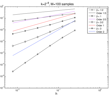
Figure 1: Spatial errors: The $L_{2}$-error in the first component decreases with order $h^{\frac{2}{3}\beta}$.

We are now interested in the time-discretisation of the above stochastic wave equation for various spatial meshes. Figure 2 displays the strong error at time $t=1$ in the first component of the solution for space-time white noise with $s=0$ and for correlated noise with $s=1/2$, respectively. One observes the order of convergence stated in Theorem 4 and the fact that these errors are independent of the spatial discretisation. Again, the exact solution is approximated by the stochastic trigonometric method with a very small step size $k_{\mathrm{exact}}=2^{-6}$. We use $h_{\mathrm{exact}}=2^{-9},2^{-10}$, resp., $2^{-11}$ for the spatial discretisations. Again $M=100$ samples are used for the approximation of the expected values.

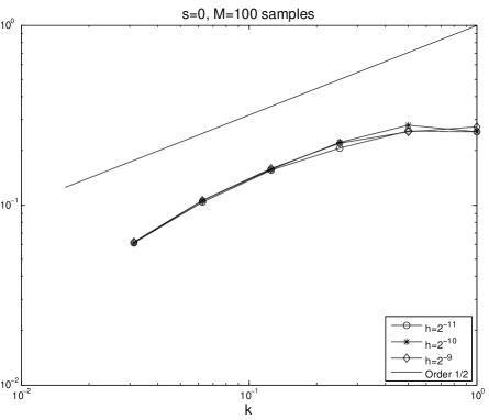
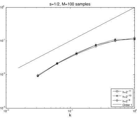
Figure 2: Temporal errors: The $L_{2}$-error in the first component decreases with order $k^{\beta}$ and is independent of the mesh-grid $h$.

Next, we compare our time integrator with the following classical numerical schemes for stochastic differential equations. When applied to the wave equation in the form (5), these schemes are:

1. The backward Euler-Maruyama scheme $X^{n+1}=X^{n}+kAX^{n+1}+B\Delta W^{n}$, see for example [15] or [22]. The strong rate of convergence for this method is $\mathcal{O}(k^{\min(\beta/2,1)})$, see [17, Theorem 4.12].

2. A stochastic version of the Störmer-Verlet scheme, writing $X=[X_{1},X_{2}]^{T}$,

   $$\begin{split}X^{n+1/2}_{2}&=X^{n}_{2}+\frac{k}{2}\Lambda X^{n}_{1}+W(t_{n+1/2})-W(t_{n}),\\ X^{n+1}_{1}&=X^{n}_{1}+kX^{n+1/2}_{2},\\ X^{n+1}_{2}&=X^{n+1/2}_{2}+\frac{k}{2}\Lambda X^{n+1}_{1}+W(t_{n+1})-W(t_{n+1/2}).\end{split}$$

   For an application of this scheme to the Langevin equation, we refer to [24]. We were not able to find any references on the strong rate of convergence of this numerical method.

3. The Crank-Nicolson-Maruyama scheme [11]

   $$X^{n+1}=X^{n}+\frac{k}{2}A(X^{n+1}+X^{n})+B\Delta W^{n}.$$

   The strong rate of convergence is $\mathcal{O}(k^{\min(2\beta/3,1)})$, see [17, Theorem 4.12].

We apply these schemes to the finite element approximation of the linear problem (16) with truncated noise. Note that both the backward Euler-Maruyama scheme and the Crank-Nicolson-Maruyama scheme are implicit. Figure 3 presents the various strong convergence rates of the above numerical integrators, once with white noise and once with correlated noise with $Q=\Lambda^{-1/2}$. One observes that the numerical solution given by the Störmer-Verlet method explodes for larger values of the step-size $k$ (this computation was stopped when the deterministic non-stable regime of the scheme was attained). For all the experiments we use $h_{\mathrm{exact}}=2^{-10}$ for the spatial discretisation. The reference solution is computed using the stochastic trigonometric method with the step size $k_{\mathrm{exact}}=2^{-16}$. Again $M=100$ samples are used.

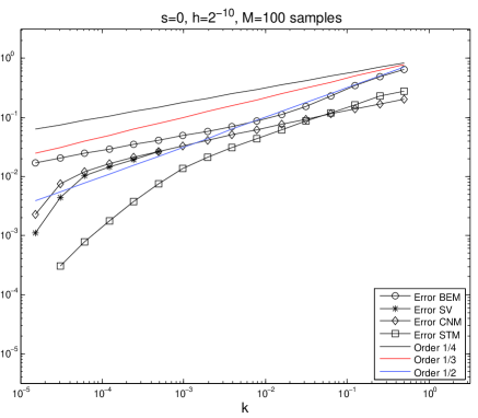
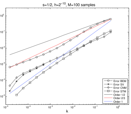
Figure 3: $L_{2}$-error in the first component of the numerical solutions given by the Störmer-Verlet method (SV), the backward Euler-Maruyama scheme (BEM), the Crank-Nicolson-Maruyama scheme (CNM) and the stochastic trigonometric method (STM).

In the following numerical experiment, we are concerned with the trace formula of Section 5. Figure 4 illustrates the trace formula of the numerical solution. Here, we choose $s=1/2$ and hence $\beta<1$ and display the expected value of the energy along the numerical solution of the above stochastic linear wave equation with mesh grids $h=0.1$ and $k=0.1$ on the long time interval $[0,500]$. We took $M=15000$ samples to approximate the expected energy of our problem. A comparison with other time integrators is presented in Figure 5. One notes that all these numerical schemes do not reproduce the linear growth of the expected energy correctly. This fact is already known for the backward Euler-Maruyama scheme applied to a finite-dimensional linear stochastic oscillator [26].

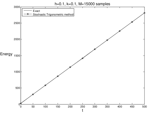
Figure 4: Trace-formula: The stochastic trigonometric method preserves exactly the linear growth of the expected value of the energy.

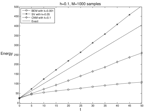
Figure 5: Although using a small time step size, the backward Euler-Maruyama scheme (BEM) does not reproduce the linear growth of the expected energy. The Störmer-Verlet method (SV) and the Crank-Nicolson-Maruyama scheme (CNM) yield better results even with a larger time step size.

Finally we consider a nonlinear stochastic wave equation, the Sine-Gordon equation driven by additive noise:

$$\mathrm{d}\dot{u}-\Delta u\,\mathrm{d}t=-\sin(u)\,\mathrm{d}t+\mathrm{d}W, \quad(x,t)\in\ (0,1)\times(0,1),$$

$$u(0,t)=u(1,t)=0, \quad t\in(0,1),$$

$$u(x,0)=0,\ \dot{u}(x,0)=1_{[\frac{1}{4},\frac{3}{4}]}(x), \quad x\in(0,1),$$

where $1_{I}(x)$ denotes the indicator function for the interval $I$. The corresponding deterministic problem is studied for example in [8]. We solve this problem again with a finite element method in space and in time we use the stochastic trigonometric method (14) with $G(X(t))=-\sin(X(t))$ and the filter functions proposed in [9]:

$$\psi(\xi)=\sin\!{\rm{c}}^{3}(\xi),\ \ \phi(\xi)=\sin\!{\rm{c}}(\xi),\ \ \psi_{0}(\xi)=\cos(\xi)\sin\!{\rm{c}}^{2}(\xi),\ \ \psi_{1}(\xi)=\sin\!{\rm{c}}^{2}(\xi),$$

where $\sin\!{\rm{c}}(\xi)=\sin(\xi)/\xi$. In the upper plot of Figure 6, we show the expected energy of the numerical solution of the Sine-Gordon equation where the covariance operator is given by $Q=I$. Even for a large step-size $k=0.1$, one can observe the good behaviour of the numerical scheme. In the lower figure, we display the convergence rate for the first component with a covariance operator $Q=\Lambda^{-1}$. Again, we approximate the exact solution with a finite element solution and the stochastic trigonometric scheme using $k_{\mathrm{exact}}=2^{-6}$ and $h_{\mathrm{exact}}=2^{-9}$.

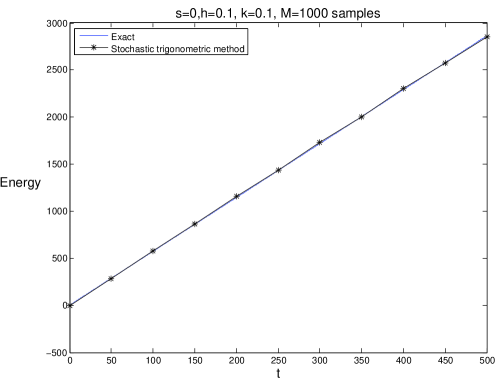
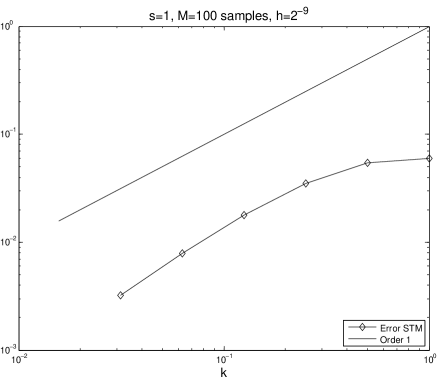
Figure 6: In the nonlinear case, the stochastic trigonometric method preserves almost exactly the linear growth of the expected value of the energy (above figure). The $L_{2}$-error in the first component of the numerical solution given by the stochastic trigonometric method decreases with order $1$.

References

• [1] Y. Cao and L. Yin, Spectral Galerkin method for stochastic wave equations driven by space-time white noise, Commun. Pure Appl. Anal., 6 (2007), pp. 607–617.
• [2] D. Cohen, On the numerical discretisation of stochastic oscillators, Math. Comput. Simul., (2012). doi:10.1016/j.matcom.2012.02.004.
• [3] D. Cohen, E. Hairer, and C. Lubich, Conservation of energy, momentum and actions in numerical discretizations of non-linear wave equations, Numer. Math., 110 (2008), pp. 113–143.
• [4] D. Cohen and M. Sigg, Convergence analysis of trigonometric methods for stiff second-order stochastic differential equations, Numer. Math., (2011). doi:10.1007/s00211-011-0426-8.
• [5] G. Da Prato and J. Zabczyk, Stochastic Equations in Infinite Dimensions, vol. 44 of Encyclopedia of Mathematics and its Applications, Cambridge University Press, Cambridge, 1992.
• [6] R. Dalang, D. Khoshnevisan, C. Mueller, D. Nualart, and Y. Xiao, A Minicourse on Stochastic Partial Differential Equations, vol. 1962 of Lecture Notes in Mathematics, Springer-Verlag, Berlin, 2009.
• [7] M. Di Paola, A. Sofi, and G. Muscolino, Nonlinear random vibrations of a suspended cable under wind loading, Proceedings of Fourth International Conference on Computational Stochastic Mechanics (CSM4), (2002), pp. 159–168.
• [8] V. Grimm, On the use of the Gautschi-type exponential integrator for wave equations, in Numerical Mathematics and Advanced Applications, Springer, Berlin, 2006, pp. 557–563.
• [9] V. Grimm and M. Hochbruck, Error analysis of exponential integrators for oscillatory second-order differential equations, J. Phys. A, 39 (2006), pp. 5495–5507.
• [10] E. Hairer, C. Lubich, and G. Wanner, Geometric Numerical Integration. Structure-Preserving Algorithms for Ordinary Differential Equations, Springer Series in Computational Mathematics 31, Springer, Berlin, 2002.
• [11] E. Hausenblas, Approximation for semilinear stochastic evolution equations, Potential Anal., 18 (2003), pp. 141–186.
• [12] M. Hochbruck and A. Ostermann, Exponential integrators, Acta Numer., 19 (2010), pp. 209–286.
• [13] A. Jentzen and P. E. Kloeden, Overcoming the order barrier in the numerical approximation of stochastic partial differential equations with additive space-time noise, Proc. R. Soc. Lond. Ser. A Math. Phys. Eng. Sci., 465 (2009), pp. 649–667.
• [14] P. E. Kloeden, G. J. Lord, A. Neuenkirch, and T. Shardlow, The exponential integrator scheme for stochastic partial differential equations: pathwise error bounds, J. Comput. Appl. Math., 235 (2011), pp. 1245–1260.
• [15] P. E. Kloeden and E. Platen, Numerical Solution of Stochastic Differential Equations, vol. 23 of Applications of Mathematics (New York), Springer-Verlag, Berlin, 1992.
• [16] M. Kovács, S. Larsson, and F. Lindgren, Weak convergence of finite element approximations of linear stochastic evolution equations with additive noise, BIT Numer. Math., 52 (2012), pp. 85–108. doi:10.1007/s10543-011-0344-2.
• [17]  , Weak convergence of finite element approximations of linear stochastic evolution equations with additive noise II. Fully discrete schemes, arXiv:1203.2029v1, (2012).
• [18] M. Kovács, S. Larsson, and F. Saedpanah, Finite element approximation of the linear stochastic wave equation with additive noise, SIAM J. Numer. Anal., 48 (2010), pp. 408–427.
• [19] G. J. Lord and J. Rougemont, A numerical scheme for stochastic PDEs with Gevrey regularity, IMA J. Numer. Anal., 24 (2004), pp. 587–604.
• [20] A. Martin, S. M. Prigarin, and G. Winkler, “Exact” numerical algorithms for linear stochastic wave equation and stochastic Klein-Gordon equation, in International Conference on Computational Mathematics. Part I, II, ICM&MG Pub., Novosibirsk, 2002, pp. 232–237.
• [21]  , Exact and fast numerical algorithms for the stochastic wave equation, Int. J. Comput. Math., 80 (2003), pp. 1535–1541.
• [22] G. N. Milstein and M. V. Tretyakov, Stochastic Numerics for Mathematical Physics, Scientific Computation, Springer-Verlag, Berlin, 2004.
• [23] C. Prévôt and M. Röckner, A Concise Course on Stochastic Partial Differential Equations, vol. 1905 of Lecture Notes in Mathematics, Springer, Berlin, 2007.
• [24] S. Reich, Smoothed Langevin dynamics of highly oscillatory systems, Phys. D, 138 (2000), pp. 210–224.
• [25] H. Schurz, Analysis and discretization of semi-linear stochastic wave equations with cubic nonlinearity and additive space-time noise, Discrete Contin. Dyn. Syst. Ser. S, 1 (2008), pp. 353–363.
• [26] A. H. Strømmen Melbø and D. J. Higham, Numerical simulation of a linear stochastic oscillator with additive noise, Appl. Numer. Math., 51 (2004), pp. 89–99.
• [27] V. Thomée, Galerkin Finite Element Methods for Parabolic Problems, vol. 25 of Springer Series in Computational Mathematics, Springer-Verlag, Berlin, second ed., 2006.
• [28] J. B. Walsh, On numerical solutions of the stochastic wave equation, Illinois J. Math., 50 (2006), pp. 991–1018 (electronic).