A Two-Stage Dimension Reduction Method for Induced Responses and Its Applications

Abstract

Researchers in the biological sciences nowadays often encounter the curse of high-dimensionality, which many previously developed statistical models fail to overcome. To tackle this problem, sufficient dimension reduction aims to estimate the central subspace (CS), in which all the necessary information supplied by the covariates regarding the response of interest is contained. Subsequent statistical analysis can then be made in a lower-dimensional space while preserving relevant information. Oftentimes studies are interested in a certain transformation of the response (the induced response), instead of the original one, whose corresponding CS may vary. When estimating the CS of the induced response, existing dimension reduction methods may, however, suffer the problem of inefficiency. In this article, we propose a more efficient two-stage estimation procedure to estimate the CS of an induced response. This approach is further extended to the case of censored responses. An application for combining multiple biomarkers is also illustrated. Simulation studies and two data examples provide further evidence of the usefulness of the proposed method.

KEY WORDS: Asymptotic efficiency, Censoring, Central subspace, Classification, Composite biomarker, Sufficient dimension reduction, SAVE, SIR, Survival.

1 Introduction

Consider the problem of inferring the association between the response $Y$ and a $p$-dimensional vector of covariates $X$. Most statistical methods perform well with a moderate size of $p$ in comparison with the sample size. Unfortunately, we have trouble in dealing with the problem when $p$ gets large, which is usually the case in the biological sciences nowadays. To improve statistical analysis, a preprocess is implemented first to reduce the number of covariates and then the subsequent statistical analysis is made based on those extracted covariates. Sufficient dimension reduction aims to reduce the number of covariates while preserving necessary information. Specifically, it searches for a matrix $\Gamma\in\textmd{R}^{p\times d}$ such that

$$Y\;\,\rule[0.0pt]{0.29999pt}{6.69998pt}\rule[0.0pt]{6.49994pt}{0.29999pt}\rule[0.0pt]{0.29999pt}{6.69998pt}\;\,X\mid\Gamma^{T}X,$$ (1)

where         stands for statistical independence and $d\leq p$. An equivalent statement is that the conditional distribution of $Y\mid X$ and $Y\mid\Gamma^{T}X$ are the same. In other words, all the information contained in $X$ regarding $Y$ can be obtained through the lower-dimensional linear transformation $\Gamma^{T}X$. Model (1) is very general without any extra specification for the conditional distribution of $Y$ given $X$. It trivially holds when $\Gamma$ is set to be the identity matrix and, hence, is useful only when $d$ is adequately small. Obviously, it is ${\rm span}(\Gamma)$ that is of interest to us, which is called the dimension reduction subspace (Cook, 1994; Li, 1991) for the regression of $Y$ on $X$. Under very general conditions, the intersection of all such dimension reduction subspaces, denoted by $\mathcal{S}_{Y\mid X}$, is still a dimension reduction subspace (Cook, 1994) and is called the central subspace (CS). We thus assume in the sequel the existence of $\mathcal{S}_{Y\mid X}={\rm span}(\Gamma)$ with structural dimension ${\rm dim}(\mathcal{S}_{Y\mid X})=d$. There have been many methodologies proposed to estimate $\mathcal{S}_{Y\mid X}$, beginning with the development of sliced inverse regression (SIR) of Li (1991), including sliced average variance estimation (SAVE) of Cook and Weisberg (1991), third-moment estimation of Yin and Cook (2003), inverse regression (IR) of Cook and Ni (2005), directional regression (DR) of Li and Wang (2007), discretization-expectation estimation of Zhu et al. (2010), among others.

Oftentimes, researchers are interested in the induced response $Y_{g}=g(Y)$ for a known function $g(\cdot)$ instead of the original one. For example, the original response $Y$ in the Cardiac Arrhythmia Study is a categorical random variable with value 1 referring to normal heart rhythm and values 2-16 for different types of arrhythmia. In the phase of population screening, however, one would merely like to distinguish patients with arrhythmia ($Y>1$) from those without it ($Y=1$). In this case, $g(Y)={I}(Y\leq 1)$ is of major interest, where ${I}(\cdot)$ is the indicator function. Taking the Angiography Cohort Study as another example, researchers aim to predict a patient’s 10-year vital status. In this study, coronary artery disease (CAD)-related death time $Y$ is the original response, and the induced response of interest is $g(Y)={I}(Y\leq 10)$. A far more complicated form of $g(\cdot)$ may, instead, be of interest, depending on the nature of the study.

Similar to (1), there must exist for every $g(\cdot)$ a $\Gamma_{g}\in\textmd{R}^{p\times d_{g}}$ such that

$$Y_{g}\;\,\rule[0.0pt]{0.29999pt}{6.69998pt}\rule[0.0pt]{6.49994pt}{0.29999pt}\rule[0.0pt]{0.29999pt}{6.69998pt}\;\,X\mid\Gamma_{g}^{T}X,$$ (2)

and one has the central subspace $\mathcal{S}_{Y_{g}\mid X}={\rm span}(\Gamma_{g})$ for the regression of $Y_{g}$ on $X$ with the structural dimension ${\rm dim}(\mathcal{S}_{Y_{g}\mid X})=d_{g}$. We must have $\mathcal{S}_{Y_{g}\mid X}\subseteq\mathcal{S}_{Y\mid X}$ since $Y_{g}$ is a function of $Y$, but a more complicated inclusion structure could exist. The following three examples demonstrate various relationships between $\mathcal{S}_{Y|X}$ and $\mathcal{S}_{Y_{g}|X}$ with $Y_{g}={I}(Y\leq t)$.

Example 1. Assume the conditional distribution of $Y$ given $X$ is

$$Y\mid X\sim\text{Gamma}(2\exp(\alpha^{T}X),~{}0.5)$$ (3)

which satisfies (1) with $\Gamma=\alpha$. It is easy to show that (2) also holds with $\Gamma_{g}=\alpha$. In this case, $\mathcal{S}_{Y_{g}\mid X}=\mathcal{S}_{Y\mid X}$ for every $t$.

Example 2. Assume the conditional distribution of $Y$ given $X$ is

$$\log Y\mid X\sim N\left(-\alpha_{1}^{T}X/\alpha_{2}^{T}X,\,(\alpha_{2}^{T}X)^{-2}\right)$$ (4)

which satisfies (1) with $\Gamma=[\alpha_{1},\,\alpha_{2}]$. Provided $\alpha_{2}^{T}X>0$, $\text{pr}(Y_{g}=1\mid X)$ is a function of $\Gamma_{g}^{T}X$, which satisfies (2) with $\Gamma_{g}=\alpha_{1}+(\log t)\alpha_{2}$. In this case, $\mathcal{S}_{Y_{g}\mid X}\subsetneq\mathcal{S}_{Y\mid X}$ and the direction of $\mathcal{S}_{Y_{g}\mid X}$ changes as $t$ varies.

Example 3. Let the conditional hazard function of $Y$ given $X$ be of the form

$$\lambda(y\mid X)={I}(y<\tau_{1})\exp(\alpha_{1}^{T}X)+{I}(\tau_{1}\leq y<\tau_{2})\exp(\alpha_{2}^{T}X)+{I}(\tau_{2}\leq y)\exp(\alpha_{3}^{T}X)$$ (5)

which satisfies (1) with $\Gamma=[\alpha_{1},\,\alpha_{2},\alpha_{3}]$. Moreover, $\text{pr}(Y_{g}=1\mid X)$ is a function of $\Gamma_{g}^{T}X$, which satisfies (2) with $\Gamma_{g}=\left[\alpha_{1},\,{I}(t\geq\tau_{1})\alpha_{2},\,{I}(t\geq\tau_{2})\alpha_{3}\right]$. In this case, $\mathcal{S}_{Y_{g}\mid X}\subseteq\mathcal{S}_{Y\mid X}$ and $\mathcal{S}_{Y_{g}\mid X}$ expands up to $\mathcal{S}_{Y\mid X}$ as $t$ increases (i.e., the dimension also changes).

These examples highlight the importance of $\mathcal{S}_{Y_{g}\mid X}$, because both the dimension and direction of the CS of $Y_{g}$ may be different from the original CS, i.e., $\mathcal{S}_{Y\mid X}$ may contain redundant directions if we are interested in $Y_{g}$ only. If we simply treat $(Y_{g},X)$ as the observed data, any dimension reduction method can be directly applied to estimate $\mathcal{S}_{Y_{g}\mid X}$. From a statistical point of view, however, $Y$ must contain more information than $Y_{g}$ does, therefore this direct method may suffer the problem of inefficiency. We use model (3) to demonstrate the potential drawback of the direct method. Set $\alpha=(1,2,0)^{T}$ and generate $X$ from $N({0}_{3},0.8\,I_{3}+0.2\,{1}_{3}{1}_{3}^{T})$, where $I_{a}$ represents the $a\times a$ identity matrix, ${1}_{a}$ and ${0}_{a}$ are $a\times 1$ vectors of ones and zeroes. Since $\mathcal{S}_{Y_{g}\mid X}=\mathcal{S}_{Y\mid X}$, SIR is implemented to estimate ${\rm span}(\Gamma_{g})$ based on $(Y,X)$ and $(Y_{g},X)$ separately with $t=t_{50}$, where $t_{a}$ satisfies $\text{pr}(Y\leq t_{a})=a\%$. The first element of the estimates is always forced to be one since only the direction is relevant. Simulation results with sample size 300 and 500 replications performed give the means and standard errors of the estimates as $(1.000,2.030\pm 0.261,0.003\pm 0.115)^{T}$ under $(Y_{g},X)$, and $(1.000,1.995\pm 0.071,0.001\pm 0.030)^{T}$ under $(Y,X)$. Although both methods can accurately estimate the true direction $(1,2,0)^{T}$, the standard errors for SIR based on $(Y_{g},X)$ are larger. We detect even larger biases and errors for other choices of $t$, especially for $t$ near the boundaries. The main theme of this paper is thus to propose a more efficient estimation procedure for $\mathcal{S}_{Y_{g}\mid X}$ based on $(Y,X)$.

2 A Two-Stage Estimation Procedure

Some notation is introduced first. For a square matrix $A$, let ${\rm Eig}(A;a)$ be the function which maps $A$ into its $a$ leading eigenvectors. The observed data $(Y_{i},X_{i})$ is a random copy of $(Y,X)$. Following the setting of Cook and Ni (2005), we may assume $Y$ has a finite support $\{1,\cdots,h\}$. In the case of a continuous response, it can be categorized as suggested by Li (1991). Let $Z=\Sigma^{-1/2}(X-\mu)$ be the standardized version of $X$, where $\mu={\rm E}[X]$ and $\Sigma={\rm cov}(X)$. Owing to $\Sigma^{-1/2}\mathcal{S}_{Y\mid Z}=\mathcal{S}_{Y\mid X}$ and $\Sigma^{-1/2}\mathcal{S}_{Y_{g}\mid Z}=\mathcal{S}_{Y_{g}\mid X}$, there is no difference in considering the dimension reduction problem under $Z$-scale. In this section, we will consider the estimation of $B$ and $B_{g}$, the basis of $\mathcal{S}_{Y\mid Z}$ and $\mathcal{S}_{Y_{g}\mid Z}$, respectively, and transform back to the original scale via $\Gamma=\Sigma^{-1/2}B$ and $\Gamma_{g}=\Sigma^{-1/2}B_{g}$. In practice, $Z$ is replaced with $\hat{Z}=\hat{\Sigma}^{-1/2}(X-\hat{\mu})$ by plugging in the usual moment estimators $\hat{\mu}$ and $\hat{\Sigma}$. The structural dimensions $d$ and $d_{g}$ are assumed to be already known. The selection of $(d,d_{g})$ will be discussed later.

We start by reviewing a general estimation procedure for $\mathcal{S}_{Y\mid Z}$. Most dimension reduction methods aim to construct a symmetric kernel matrix $K$ (if $K$ is not symmetric, $KK^{T}$ is used instead) based on $(Y,X)$ satisfying the property

$${\rm span}(K)=\mathcal{S}_{Y\mid Z}.$$ (6)

A basis of $\mathcal{S}_{Y\mid Z}$ is then given by $B={\rm Eig}(K;d)$. At the sampling level, $B$ is estimated by $\hat{B}={\rm Eig}(\hat{K};d)$, where $\hat{K}$ is a sample analogue of $K$. For example, SIR considers

$$K_{\rm SIR}=\Sigma^{-1/2}M\Sigma^{-1/2},~{}~{}~{}M={\rm cov}({\rm E}[X\mid Y])=({m}-\mu{1}_{h}^{T})D_{f}({m}-\mu{1}_{h}^{T})^{T},$$ (7)

where ${m}=[m_{1},\cdots,m_{h}]$ with $m_{i}={\rm E}[X\mid Y=i]$, ${f}=(f_{1},\cdots,f_{h})$ with $f_{i}=\text{pr}(Y=i)$, and $D_{f}=\text{diag}({f})$. A sample analogue $\hat{K}_{\rm SIR}$ is obtained by plugging the moment estimators $\hat{m}$, $\hat{f}$, $\hat{\mu}$, and $\hat{\Sigma}$ into $K_{\rm SIR}$. It should be noted that property (6) does not hold without any cost. Depending on the choice of $K$, different conditions are imposed to ensure its validity. Inverse regression methods, such as SIR, commonly assume the linearity condition ((A1): ${\rm E}[Z\mid A^{T}Z]$ is a linear function of $Z$ for any matrix $A$), which is equivalent to assuming the ellipticity of $X$ (Eaton, 1986).

Turning to the estimation of $\mathcal{S}_{Y_{g}\mid Z}$ for any given $g(\cdot)$, parallel to (6), based on $(Y_{g},X)$ we find the symmetric kernel matrix $K_{g}$ satisfying

$${\rm span}(K_{g})=\mathcal{S}_{Y_{g}\mid Z},$$ (8)

and the basis of $\mathcal{S}_{Y_{g}\mid Z}$ which is of major interest is defined to be $B_{g}={\rm Eig}(K_{g};d_{g})$. The direct estimation method then substitutes an estimator $\hat{K}_{g}$ for $K_{g}$, and estimates $B_{g}$ by ${\rm Eig}(\hat{K}_{g};d_{g})$. Similar to (7), $K_{g}$ of SIR is given by

$$K_{g,\rm SIR}=\Sigma^{-1/2}M_{g}\Sigma^{-1/2},~{}~{}~{}M_{g}={\rm cov}({\rm E}[X\mid Y_{g}])=({m}_{g}-\mu{1}_{s}^{T})D_{{f}_{g}}({m}_{g}-\mu{1}_{s}^{T})^{T},$$ (9)

where ${m}_{g}=[m_{g1},\cdots,m_{gs}]$, $m_{gi}={\rm E}[X\mid Y_{g}=i]$, ${f}_{g}=(f_{g1},\cdots,f_{gs})$, $f_{gi}=\text{pr}(Y_{g}=i)$, and $s$ is the number of categories of $Y_{g}$. Note that $s\leq h$ since $Y_{g}$ is a function of $Y$. The sample analogue $\hat{K}_{g,\rm SIR}$ can be obtained by plugging the moment estimators $\hat{m}_{g}$, $\hat{f}_{g}$, $\hat{\mu}$, and $\hat{\Sigma}$ into $K_{g,\rm SIR}$. We have seen in the end of Section 1 that direct estimation based on $(Y_{g},X)$ may lose information, and we attempt to propose a more efficient estimation procedure. First observe that under the validity of (6) and (8), we must have

$$K_{g}=P_{B}K_{g}P_{B},$$ (10)

where $P_{B}=BB^{T}$ is the orthogonal projection matrix onto ${\rm span}(B)$. Although (10) is straightforward, it motivates us to estimate $K_{g}$ by $\hat{P}_{B}\hat{K}_{g}\hat{P}_{B}$, where $\hat{P}_{B}=\hat{B}\hat{B}^{T}$ is an estimate of $P_{B}$. It is the projection $\hat{P}_{B}$ that utilizes the extra information in $(Y,X)$, and results in an expected gain in efficiency. Details of the procedure are listed below:

• Based on $(Y,X)$, apply a dimension reduction method to obtain $\hat{K}$ and, hence, $\hat{P}_{B}$.

• Based on $(Y_{g},X)$, apply a dimension reduction method to obtain $\hat{K}_{g}$.

• Estimate $B_{g}$ by $\hat{B}_{g}={\rm Eig}(\hat{P}_{B}\hat{K}_{g}\hat{P}_{B};d_{g})$.

With $\hat{B}_{g}$ obtained, we then estimate a basis of $\mathcal{S}_{Y_{g}|X}$, say $\Gamma_{g}$, by $\hat{\Gamma}_{g}=\hat{\Sigma}^{-1/2}\hat{B}_{g}$. The $n^{1/2}$-consistency of $\hat{\Gamma}_{g}$ is a direct consequence provided $\hat{K}$ and $\hat{K}_{g}$ are also $n^{1/2}$-consistent. We call the two-stage estimation procedure “A-B” hereafter, if method A is used in Step 1 and method B in Step 2. As SIR is the most widely applied dimension reduction method, the following theorem, which guarantees that SIR-SIR is more efficient than SIR, highlights the desirability of using our two-stage estimation procedure. We use “acov” to denote the asymptotic covariance, and $A\geq 0$ to indicate $A$ is positive semi-definite. The proof is deferred to the Appendix.

Theorem 1.

Let $\hat{\Gamma}_{g}$ be obtained from SIR-SIR, and let $\tilde{\Gamma}_{g}=\hat{\Sigma}^{-1/2}{\rm Eig}(\hat{K}_{g,\rm SIR};d_{g})$ be the direct estimate of $\Gamma_{g}$ from SIR. In addition to the linearity condition (A1) above, assume the validity of (A2): ${\rm cov}(\nu^{T}Z\mid B^{T}Z)$ is non-random for any $\nu\bot~{}\mathcal{S}_{Y\mid Z}$. Then,

$$\Delta={\rm acov}\left(n^{1/2}{\rm vec}(\tilde{\Gamma}_{g}-\Gamma_{g})\right)-{\rm acov}\left(n^{1/2}{\rm vec}(\hat{\Gamma}_{g}-\Gamma_{g})\right)\geq 0.$$

The equality holds if and only if ${\rm span}(K_{g,\rm SIR})\bigcap~{}{\rm span}(K_{\rm SIR}-K_{g,\rm SIR})=\{0\}$, where $K_{\rm SIR}$ and $K_{g,\rm SIR}$ are defined in (7) and (9).

In the establishment of Theorem 1, in addition to the linearity condition we require ${\rm cov}(\nu^{T}Z\mid B^{T}Z)$ to be non-random for any $\nu$ in the complement of $\mathcal{S}_{Y\mid Z}$. These conditions are not that restrictive and can be generally satisfied. As argued by Li and Wang (2007), (A1)-(A2) are shown to approximately hold when $p$ is large. Moreover, (A2) is valid when $X$ is normally distributed. Although normality is a stronger condition, it can be approximated by making a power transformation of $X$. One implication of Theorem 1 is that the total asymptotic variance of $\tilde{\Gamma}_{g}$ is strictly larger than that of $\hat{\Gamma}_{g}$ provided $\Delta\neq 0$. The only possibility of no efficiency gain (i.e., $\Delta=0$) is when ${\rm span}(K_{g,\rm SIR})$ and ${\rm span}(K_{\rm SIR}-K_{g,\rm SIR})$ have no common element except the zero point. This is reasonable since, under this situation, all the information about $S_{Y_{g}|Z}$ contained in $K_{\rm SIR}$ resides in $K_{g,\rm SIR}$ and knowing the “residual” $(K_{\rm SIR}-K_{g,\rm SIR})$ contributes nothing to the construction of $S_{Y_{g}|Z}$. Hence, we will gain nothing from SIR-SIR. A formal test for this condition is beyond the scope of this article and will be investigated in a future study. In summary, SIR-SIR is expected to perform well in most of the situations except the rather restrictive special case. This fact is also demonstrated by our simulation studies in Section 4, where the efficiency gain of the two-stage method is obviously detected.

The structural dimensions $d$ and $d_{g}$ should be determined before practical implementation. To estimate $d$, most methods rely on a sequence of hypothesis tests (Li, 1991; Cook and Lee, 1999, Cook and Yin, 2001). These methods, however, may not be readily applicable for the selection of $d_{g}$. To simplify the estimation procedure, we alternatively suggest two approaches to select $(d,d_{g})$. One is to adopt the maximal eigenvalue ratio criterion (MERC) proposed by Luo, Wang, and Tsai (2009). Let $\hat{\lambda}_{i}$ be the eigenvalue of $\hat{K}$ and define $\hat{\rho}_{i}=\hat{\lambda}_{i}/\hat{\lambda}_{i+1}$ for $1\leq i\leq p-1$. It is proposed to select $d$ by $\hat{d}=\arg\max_{1\leq i\leq d^{*}}\hat{\rho}_{i}$, where $d^{*}$ is a pre-specified constant. The authors suggest using $d^{*}=5$ in practice. Once $\hat{d}$ is obtained, we can estimate $d_{g}$ by a similar procedure. Let $\hat{\lambda}_{g,i}$ be the eigenvalue of $\hat{P}_{B}\hat{K}_{g}\hat{P}_{B}$ and define $\hat{\rho}_{g,i}=\hat{\lambda}_{g,i}/\hat{\lambda}_{g,i+1}$ for $1\leq i\leq\hat{d}-1$. Then $d_{g}$ is determined by $\hat{d}_{g}=\arg\max_{1\leq i\leq\hat{d}-1}\hat{\rho}_{g,i}$. As to the second method, note that the purpose of dimension reduction is to improve regression or classification. Thus, it is natural to select $(d,d_{g})$ so that a measure of classification accuracy is maximized. In Section 5 below, the classification accuracy obtained from cross-validation is used in the Cardiac Arrhythmia Study, while the AUC (area under the receiver operating characteristic (ROC) curve) is considered in the Angiography Cohort Study to select $(d,d_{g})$.

Remark 1.

In our two motivating examples, $Y_{g}={I}(Y\leq t)$ is binary and, hence, due to its nature, SIR can capture at most one direction of $\mathcal{S}_{Y_{g}\mid Z}$. Alternatively, we can adopt SAVE in Step 2. Cook and Lee (1999) showed that for a binary response, SAVE is more comprehensive than SIR. The kernel matrix of SAVE is

$$K_{g,\rm SAVE}=\left[\Sigma^{-1/2}(\mu_{t1}-\mu_{t0})~{},\Sigma^{-1/2}(\Sigma_{t1}-\Sigma_{t0})\Sigma^{-1/2}\right]$$ (11)

with $\mu_{ti}=E[X\mid Y_{g}=i]$ and $\Sigma_{ti}={\rm cov}(X\mid Y_{g}=i)$, $i=0,1$. Its sample analogue $\hat{K}_{g,\rm SAVE}$ is obtained by plugging moment estimators $\hat{\mu}_{t0}$, $\hat{\mu}_{t1}$, $\hat{\Sigma}_{t0}$, $\hat{\Sigma}_{t1}$, and $\hat{\Sigma}$ into (11).

3 Extension to Censored Response

Dimension reduction is usually applied in the field of life science when the response of interest $Y$ represents the survival time of a subject. An important issue in survival analysis is that the response may be censored. The exact survival time $Y$ (and hence $Y_{g}$) may not always be observed and we can only observe $(Y^{*},\delta,X)$ instead, where $Y^{*}=\min\{Y,C\}$ is the last observed time, $\delta={I}(Y\leq C)$ is the censoring status, and $C$ is the censoring time. Motivated from two data examples in Section 1, our aim here is to modify SIR-SAVE to estimate $\mathcal{S}_{Y_{g}\mid X}$ with the specific choice $Y_{g}={I}(Y\leq t)$ under the validity of totally independent censorship $C\;\,\rule[0.0pt]{0.29999pt}{6.69998pt}\rule[0.0pt]{6.49994pt}{0.29999pt}\rule[0.0pt]{0.29999pt}{6.69998pt}\;\,(Y,X)$. The modified SIR-SIR will also be illustrated. We note that totally independent censorship is satisfied in the Angiography Cohort Study, since most of the patients are subject to Type-I censoring.

Both SIR and SAVE in Steps 1-2 should therefore be modified. For SIR in Step 1, observe that $\mathcal{S}_{(Y^{*},\delta)\mid Z}\subseteq\mathcal{S}_{(Y,C)\mid Z}=\mathcal{S}_{Y\mid Z}$, where the first inclusion property holds since $(Y^{*},\delta)$ is a function of $(Y,C)$, and the last equality is true by the totally independent censorship assumption. Thus, we suggest using the modified kernel matrix

$$K_{\rm SIR}^{*}=\Sigma^{-1/2}M^{*}\Sigma^{-1/2},~{}~{}~{}M^{*}={\rm cov}({\rm E}[X\mid Y^{*},\delta])=({m}^{*}-\mu{1}_{h_{0}+h_{1}}^{T})D_{{f}^{*}}({m}^{*}-\mu{1}_{h_{0}+h_{1}}^{T})^{T},$$

where ${m}^{*}=[m_{(0,1)}^{*},\cdots,m_{(0,h_{0})}^{*},m_{(1,1)}^{*},\cdots,m_{(1,h_{1})}^{*}]$ with $m_{(i,j)}^{*}={\rm E}[X\mid\delta=i,Y^{*}=j]$, ${f}^{*}=(f_{(0,1)}^{*},\cdots,f_{(0,h_{0})}^{*},f_{(1,1)}^{*},\cdots,f_{(1,h_{1})}^{*})^{T}$ with $f_{(i,j)}^{*}=\text{pr}(\delta=i,Y^{*}=j)$, and $h_{0}\leq h$ and $h_{1}\leq h$ denote the number of categories of $Y^{*}$ when $\delta=0$ and $\delta=1$. Here the slice means, the $m_{(i,j)}^{*}$’s, are formed within those patients with $\delta=0$ and $\delta=1$ separately. By plugging in moment estimators $\hat{m}^{*}$, $\hat{f}^{*}$, $\hat{\mu}$, and $\hat{\Sigma}$, the sample analogue $\hat{K}_{\rm SIR}^{*}$ is obtained. This double slicing procedure was originally proposed by Li, Wang, and Chen (1999), and our point is to emphasize its validity under totally independent censorship.

With regard to implementing SAVE in Step 2, we can still use the kernel matrix $K_{g,\rm SAVE}$ in (11) provided it can be estimated based on $(Y^{*},\delta,X)$. First observe that

$$E[X^{\otimes i}\mid Y_{g}=0]=-\frac{\int u^{\otimes i}dS_{XY}(u,t)}{S_{XY}(-\infty,t)},~{}i=1,2,$$ (12)

$$E[X^{\otimes i}\mid Y_{g}=1]=-\frac{\int u^{\otimes i}d\{S_{XY}(u,-\infty)-S_{XY}(u,t)\}}{1-S_{XY}(-\infty,t)},~{}i=1,2,$$ (13)

where $a^{\otimes 1}=a$ and $a^{\otimes 2}=aa^{T}$ for a vector $a$, and $S_{XY}(x,y)={\rm pr}(X>x,Y>y)$. Here “$>$” is interpreted as component-wise for a vector. It implies the $\mu_{ti}$’s and $\Sigma_{ti}$’s in (11) are functionals of $S_{XY}(x,y)$. Campbell (1981) and Burke (1988) have separately proposed two different estimators of $S_{XY}(x,y)$, denoted by $\hat{S}^{(c)}_{XY}(x,y)$ and $\hat{S}^{(b)}_{XY}(x,y)$. By plugging $\hat{S}_{XY}^{(c)}(x,y)$ into (12) and $\hat{S}_{XY}^{(b)}(x,y)$ into (13), we can estimate $\mu_{ti}$’s and $\Sigma_{ti}$’s by

$$\hat{\mu}_{t0}^{*}=\frac{\sum_{i=1}^{n}X_{i}{I}(Y_{i}^{*}>t)}{\sum_{i=1}^{n}{I}(Y^{*}_{i}>t)}, \hat{\Sigma}_{t0}^{*}=\frac{\sum_{i=1}^{n}X_{i}^{\otimes 2}{I}(Y_{i}^{*}>t)}{n\hat{S}_{Y}(t)}-\{\hat{\mu}_{t0}^{*}\}^{\otimes 2},$$

$$\hat{\mu}_{t1}^{*}=\frac{1}{n}\sum_{i=1}^{n}\frac{X_{i}\delta_{i}{I}(Y_{i}^{*}\leq t)}{\{1-\hat{S}_{Y}(t)\}\hat{S}_{C}(Y_{i}^{*})}, \hat{\Sigma}_{t1}^{*}=\frac{1}{n}\sum_{i=1}^{n}\frac{X_{i}^{\otimes 2}\delta_{i}{I}(Y_{i}^{*}\leq t)}{\{1-\hat{S}_{Y}(t)\}\hat{S}_{C}(Y_{i}^{*})}-\{\hat{\mu}_{t1}^{*}\}^{\otimes 2},$$

where $\hat{S}_{Y}(y)$ and $\hat{S}_{C}(y)$ are Kaplan-Meier estimators of $\text{pr}(Y>y)$ and $\text{pr}(C>y)$. Finally, a modified estimator of $K_{g,\rm SAVE}$ is given by

$$\hat{K}_{g,\rm SAVE}^{*}=\left[\hat{\Sigma}^{-1/2}(\hat{\mu}_{t1}^{*}-\hat{\mu}_{t0}^{*})~{},\hat{\Sigma}^{-1/2}(\hat{\Sigma}_{t1}^{*}-\hat{\Sigma}_{t0}^{*})\hat{\Sigma}^{-1/2}\right].$$

The modified SIR-SAVE is then proposed by using $\hat{K}_{\rm SIR}^{*}$ and $\hat{K}_{g,\rm SAVE}^{*}$ in Steps 1-2.

Remark 2.

For binary $Y_{g}$, Cook and Lee (1999) showed that the population kernel matrix of SIR can be expressed as $\Sigma^{-1/2}(\mu_{t1}-\mu_{t0})$. The modified SIR-SIR is then proposed by using $\hat{K}_{g,\rm SIR}^{*}=\hat{\Sigma}^{-1/2}(\hat{\mu}_{t1}^{*}-\hat{\mu}_{t0}^{*})$ in Step 2.

4 Simulation Studies

We use models (4)-(5) to evaluate the performance of our two-stage estimation procedure under different combinations of sample sizes $(n=50,100)$, number of covariates $(p=10,20)$, and censoring rates (${\rm CR}=0\%,25\%$). With censored data, the modified procedure is implemented instead. To measure the closeness of two spaces with basis $A$ and $A^{\prime}$, we adopt the Frobenius norm $\text{tr}\{(P_{A}-P_{A^{\prime}})(P_{A}-P_{A^{\prime}})\}^{1/2}$, where $P_{A}$ is the orthogonal projection matrix onto ${\rm span}(A)$. Simulations are repeated 500 times.

For model (4), set $\alpha_{1}=(3,0.9,-1.5,{0}_{p-3}^{T})^{T}$ and $\alpha_{2}=(3,4.5,6,{0}_{p-3}^{T})^{T}$. We independently generate $u$ and $r$ from $N_{p}(0,I_{p})$ and Beta$(1.8,0.3)$, and define $X=\mu+\Sigma^{1/2}ru(u^{T}u)^{-1/2}$ with $\Sigma=0.8I_{p}+0.2{1}_{p}{1}_{p}^{T}$ and $\mu=(0,3,0,{0}_{p-3}^{T})^{T}$. This ensures the ellipticity of $X$. For the censored case, $C$ is generated from Gamma$(2,1.71)$ so that CR$=25\%$. Both SIR-SIR and SIR are implemented at $t=t_{30}$, $t_{50}$, and $t_{70}$. As for the case of model (5), we set $\alpha_{1}=(20,0,0,{0}_{p-3}^{T})^{T}$, $\alpha_{2}=(0,15,0,{0}_{p-3}^{T})^{T}$, $\alpha_{3}=(0,0,10,{0}_{p-3}^{T})^{T}$, and $(\tau_{1},\tau_{2})=(\log 2,\log 8)$, generate $X$ from $N_{p}(-0.2\cdot{1}_{p},D(0.8I_{p}+0.2\cdot{1}_{p}{1}_{p}^{T})D)$ with $D={\rm diag}(2,1,1,{1}_{p-3}^{T})$, and generate $C$ from Gamma(1,8) to produce CR$=25\%$. We implement SIR-SAVE and SAVE at $t=t_{45}$, $t_{65}$, and $t_{75}$ so that $d_{g}=1$, 2, and 3. Various choices of the slicing number were examined and produced a similar result. We thus use $h=10$ for SIR-SIR and SIR-SAVE, and $(h_{0},h_{1})=(5,10)$ for the modified methods.

Simulation results are provided in Table 1. Compared with the standard setting $(n,p,{\rm CR})=(100,10,0\%)$, an overall observation is that SIR-SIR and SIR-SAVE outperform SIR and SAVE, even for the cases of smaller sample size $(n=50)$, of more “noise” covariates $(p=20)$, and of censored response (CR$=25\%$). The magnitude of efficiency gain from SIR-SIR is roughly the same for every $t$ in model (4). Interestingly, the efficiency gain from SIR-SAVE in model (5) becomes greater for larger $t$. One reason is that the structural dimension of $\mathcal{S}_{Y_{g}|X}$ also increases as $t$ does. With more directions needing to be estimated, more information is required to recover $\mathcal{S}_{Y_{g}|X}$, and we gain more from the two-stage estimation procedure. It has been found empirically that SAVE is less efficient than SIR. Li and Zhu (2007) showed that SAVE will not attain $n^{1/2}$-consistency in general, while SIR will, even if the number of samples in each slice is only 2. By combining SIR and SAVE, we expect an efficiency gain from SIR-SAVE as shown in this simulation.

5 Data Examples

5.1 The Angiography Cohort Study

Detailed description of the data can be found in Lee et al. (2006). Briefly speaking, for each of 1050 traceable patients, four biomarkers (CRP, SAA, IL-6, and tHcy) and the CAD-related time of death were recorded with the aim of using the combined biomarkers to accurately predict a patient’s $t$-year vital status, and thus the induced response of interest is $Y_{g}={I}(Y\leq t)$. Hung and Chiang (2010) analyzed this data, combining biomarkers via the extended generalized linear model (EGLM): $P(Y\leq t\mid X)=G(t,\beta_{t}^{T}X)$, where $\beta_{t}$ is a $p\times 1$ time-varying coefficient vector and $G(\cdot,\cdot)$ is an unknown link function which is monotone increasing in its two arguments. Under EGLM, $\beta_{t}^{T}X$ is promised to be optimal in distinguishing $\{Y\leq t\}$ from $\{Y>t\}$, in the sense that the time-dependent ROC curve (Heagerty, Lumley, and Pepe, 2000) is the highest among all functions of $X$.

The EGLM also satisfies (2) with $Y_{g}={I}(Y\leq t)$, $\mathcal{S}_{Y_{g}|X}={\rm span}(\Gamma_{g})={\rm span}(\beta_{t})$, and $d_{g}=1$. Thus, $\Gamma_{g}^{T}X$ is also the optimal biomarker since any monotone transformation of $\beta_{t}^{T}X$ will have the same time-dependent ROC curve. Given that a censoring mechanism is involved in this study, the modified SIR-SIR is applied to obtain $\hat{\Gamma}_{g}$ in order to combine the biomarkers. We enter the transformed biomarker $X_{i}/\text{sd}(X_{i})$ to perform our analysis. The analysis results with $d=3$ and $(h_{0},h_{1})=(2,4)$ are found in Table 2. We remind the reader that the choice of these tuning parameters attains the maximum of the time-dependent AUC as mentioned in Section 2. The absolute coefficient of CRP is smallest at the beginning and increases as time goes by. SAA has a totally different behavior, where it has a larger effect initially but seems to be diminishing at 3500 days. Both IL-6 and tHcy are found to play important roles in predicting patient’s vital status over time. Interestingly, CRP has a reverse effect as compared with the other three biomarkers. Table 2 provides the time-dependent AUC of the composite biomarkers $\hat{\Gamma}_{g}^{T}X$ at day $t$, denoted by $\mathcal{A}_{t}$ (see equation (8) of Chiang and Hung, 2010). The larger the $\mathcal{A}_{t}$ values, the higher prediction power $\hat{\Gamma}_{g}^{T}X$ has. One can see that most of the $\mathcal{A}_{t}$ values are greater than 0.7, especially at the beginning of the study. We also calculated $\mathcal{A}_{t}^{*}$ values, the maximal time-dependent AUC of the method developed in Hung and Chiang (2010), and a similar pattern to that of the $\mathcal{A}_{t}$ values was detected (note that $\mathcal{A}_{t}\leq\mathcal{A}_{t}^{*}$ will always hold for every $t$). In summary, SIR-SIR is easy to implement and achieves acceptable AUC values.

5.2 The Cardiac Arrhythmia Study

The study consisted of 452 patients, each with 279 covariates. The response $Y\in\{1,\cdots,16\}$ is a categorical random variable, where 1 refers to “normal” and 2-16 refer to different classes of arrhythmia. See Güvenir et al. (1997) for details.

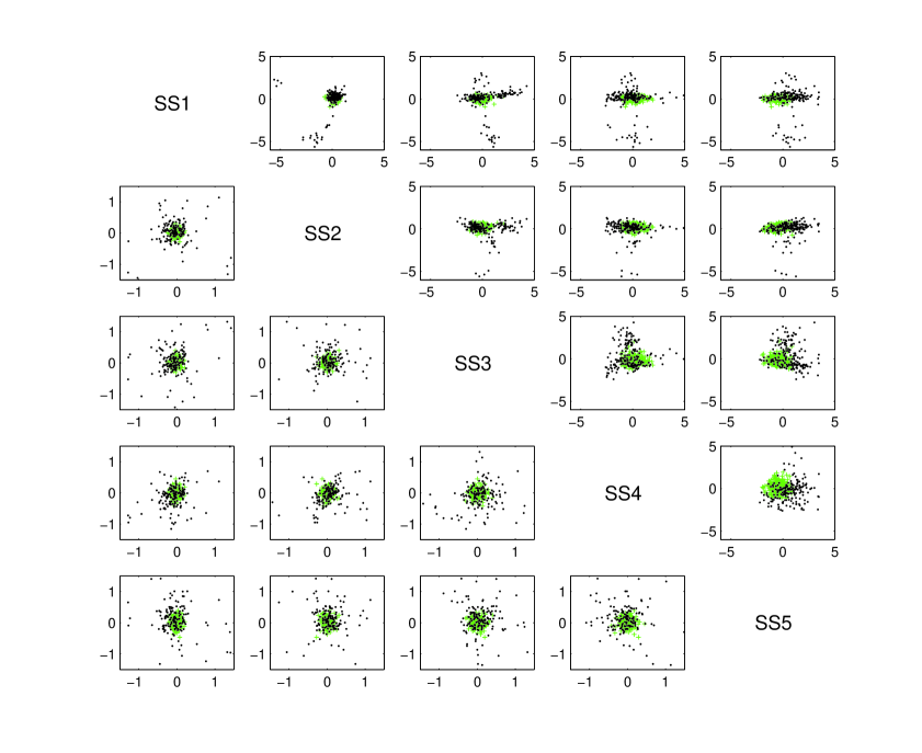
Figure 1: The scatter plot matrix of extracted predictors from SIR-SAVE (upper triangular panel) and SAVE (lower triangular panel) with $(d,d_{g})=(7,5)$. The green pluses and black dots indicate the normal and abnormal patients.

To keep matters simple, we consider continuous predictors only and use their first 100 principal components in our analysis. We are interested in distinguishing normal patients $\{Y=1\}$ from abnormal ones $\{Y>1\}$, i.e., $Y_{g}={I}(Y\leq 1)$. The scatterplots of the extracted predictors (denoted by SS1,$\cdots$,SS5) from SIR-SAVE with $(d,d_{g})=(7,5)$ are provided in Figure 1. Again, the selection of $(d,d_{g})$ is such that the averaged classification accuracy from cross-validation is maximized. It can be seen that SS1-SS3 demonstrate their ability to separate two groups via variation, while SS4-SS5 attempt to separate two groups via location. In every subplot, the normal group seems to have smaller variation and locates in the center of a relatively large data cloud of the abnormal group. The bottom-left 10 subplots of Figure 1 are scatterplots of those extracted predictors taken from SAVE directly. It can be seen that there is only a separation pattern of variation between the two groups, but no obvious location difference. To further evaluate the performance of those extracted predictors, we randomly separate the data into a training set ($90\%$) and a test set ($10\%$), and then implement quadratic discriminant analysis based on those extracted predictors. The procedure with 200 replications gives SIR-SAVE the averaged classification accuracy of $78\%$, while it is a mere $70\%$ for SAVE.

6 Discussion

Although we have considered univariate responses only, there is nothing different about carrying out the procedure with multivariate responses, except that the kernel matrices $\hat{K}$ and $\hat{K}_{g}$ are constructed for multivariate responses $Y$ and $g(Y)$. A multivariate response version of Theorem 1 can be derived with a proof analogous to the proof of the univariate case. We refer to Li, Wen, and Zhu (2008) for some recent developments in dimension reduction with multivariate responses. We note that the proposed two-stage estimation procedure is a general framework, and is not limited to any specific method. Depending on the purpose of a given study, we may adopt any dimension reduction technique in either Steps 1 or 2 of the procedure. Besides SIR-SIR and SIR-SAVE, we also tested various combinations of SIR, SAVE, IR, and DR. Simulation results (not shown here) all convey the same message that an efficiency gain is significantly detected, which provides evidence that the superiority of the two-stage procedure comes mainly from using $\hat{P}_{B}\hat{K}_{g}\hat{P}_{B}$, and is not limited to any specific choice of dimension reduction method.

REFERENCES

Anderson, W. N., Jr. and Duffin, R. J. (1969). Series and parallel addition of matrices. J. Math. Anal. Appl. 26, 576-594.

Burke, M. D. (1988). Estimation of a bivariate distribution function under random censorship. Biometrika 75, 379-382.

Campbell, G. (1981). Nonparametric bivariate estimation with randomly censored data. Biometrika 68, 417-423.

Chiang, C. T. and Hung, H. (2010). Nonparametric estimation for time-dependent AUC. J. Stat. Plan. Infer. 140, 1162-1174.

Cook, R. D. and Weisberg, S. (1991). Discussion of “Sliced inverse regression for dimension reduction”. J. Am. Stat. Assoc. 86, 328-332.

Cook, R. D. (1994). On the interpretation of regression plots. J. Am. Stat. Assoc. 89, 177-189.

Cook, R. D. and Lee, H. (1999). Dimension reduction in binary response regression. J. Am. Stat. Assoc. 94, 1187-1200.

Cook, R. D. Yin, X. (2001). Dimension reduction and visualization in discriminant analysis (with discussion). Aust. Nz. J. Stat. 43, 147-199.

Cook, R. D. and Ni, L. (2005). Sufficient dimension reduction via inverse regression: a minimum discrepancy approach. J. Am. Stat. Assoc. 100, 410-427.

Eaton, M. L. (1986). A characterization of spherical distributions. J. Multivariate Anal. 20, 272-276.

Güvenir, H. A., Acar, B., Demiröz, G, and Çekin, A. (1997). A supervised machine learning algorithm for arrhythmian analysis. Computers in Cardiology 24, 433-436.

Heagerty, P. J., Lumley, T. and Pepe, M. (2000). Time-dependent ROC curves for censored survival data and a diagnostic marker. Biometrics 56, 337-344.

Hung, H. and Chiang, C. T. (2010). Optimal composite markers for time-dependent receiver operating characteristic curves with censored survival data. Scand. J. Stat. 37, 664-679.

Lee, K. W. J., Hill, J. S., Walley, K. R., and Frohlich, J. J. (2006). Relative value of multiple plasma biomarkers as risk factors for coronary artery disease and death in an angiography cohort. Canadian Medical Association Journal 174, 461-466.

Li, B. and Wang, S. (2007). On directional regression for dimension reduction. J. Am. Stat. Assoc. 102, 997-1008.

Li, B., Wen, S. and Zhu, L. (2008). On a projective resampling method for dimension reduction with multivariate responses. J. Am. Stat. Assoc. 103, 1177-1186.

Li, K. C. (1991). Sliced inverse regression for dimension reduction (with discussion). J. Am. Stat. Assoc. 86, 316-342.

Li, K. C., Wang, J. L., and Chen, C. H. (1999). Dimension reduction for censored regression data. Ann. Stat. 27, 1-23.

Li, Y. X. and Zhu, L. X. (2007). Asymptotics for sliced average variance estimation. Ann. Stat. 35, 41-69.

Luo, R., Wang, H., and Tsai, C. L. (2009). Contour projected dimension reduction. Ann. Stat. 37, 3743-3778.

Saracco, J. (1997). An asymptotic theory for sliced inverse regression. Commun. Stat. - Theor. M. 26, 2141-2171.

Tyler, D. E. (1981). Asymptotic inference for eigenvectors. Ann. Stat. 9, 725-736.

Yin, X. and Cook, R. D. (2003). Estimating the central subspaces via inverse third moments. Biometrika 90, 113-125.

Zhu, L., Wang, T., Zhu, L., and Ferré, L. (2010). Sufficient dimension reduction through discretization-expectation estimation. Biometrika 97, 295-304.

APPENDIX

Let $\Sigma_{i}={\rm cov}[X\mid Y=i]$, $\Sigma_{gj}={\rm cov}[X\mid Y_{g}=j]$, ${J}=(J_{1},\cdots,J_{h})^{T}$ with $J_{i}={I}(Y=i)$, ${J}_{g}=(J_{g1},\cdots,J_{gs})^{T}$ with $J_{gj}={I}(Y_{g}=j)$, ${\rm E}[{J}]={f}$, and ${\rm E}[{J}_{g}]={f}_{g}$. There must exist a code matrix $G=[G_{1},\cdots,G_{s}]$ with $G_{i}\in\mathbb{R}^{h}$ containing only zeros and ones such that ${J}_{g}=G^{T}{J}$. We may assume $\mu=0$ without loss of generality and, hence, $M={m}D_{f}{m}^{T}$ and $M_{g}={m}_{g}D_{{f}_{g}}{m}_{g}^{T}$. From the definitions of $K_{\rm SIR}$ and $K_{g,\rm SIR}$, we have $\Gamma={\rm Eig}(\Sigma^{-1}M;d)$ and $\Gamma_{g}={\rm Eig}(\Sigma^{-1}M_{g};d_{g})$. Similarly, $\hat{\Gamma}={\rm Eig}(\hat{\Sigma}^{-1}\hat{M};d)$, $\tilde{\Gamma}_{g}={\rm Eig}(\hat{\Sigma}^{-1}\hat{M}_{g};d_{g})$, and $\hat{\Gamma}_{g}={\rm Eig}(\hat{\Sigma}^{-1}\hat{P}^{T}\hat{M}_{g}\hat{P};d_{g})$, where $\hat{P}=\hat{\Gamma}\hat{\Gamma}^{T}\hat{\Sigma}$ is an estimator of $P=\Gamma\Gamma^{T}\Sigma$ which is the projection matrix onto ${\rm span}(\Gamma)$ relative to the $\Sigma$-inner product.

Proof of Theorem 1.

By $P^{T}M_{g}P=M_{g}$ and delta method, it suffices to show

$$\Psi={\rm acov}\left(U_{n}^{*}\right)-{\rm acov}\left(U_{n}\right)\geq 0,$$

where $U_{n}=n^{1/2}{\rm vec}(\hat{\Sigma}^{-1}\hat{P}^{T}\hat{M}_{g}\hat{P}-\Sigma^{-1}M_{g})$ and $U_{n}^{*}=n^{1/2}{\rm vec}(\hat{\Sigma}^{-1}\hat{M}_{g}-\Sigma^{-1}M_{g})$. We first derive the weak convergence of $U_{n}$. Let $H_{0}(M,M_{g},\Sigma)=\Sigma^{-1}P^{T}M_{g}P$. One has $H=\partial{\rm vec}(H_{0}(M,M_{g},\Sigma))/\partial{\rm vec}([M,M_{g},\Sigma])=[H_{1},H_{2},H_{3}]$ by Lemma 4.1 of Tyler (1981), where $H_{1}=(I_{p}\otimes\Sigma^{-1})(I_{p^{2}}+T_{p,p})\{Q^{T}\otimes(M_{g}M^{+})\}$, $H_{2}=P^{T}\otimes(\Sigma^{-1}P^{T})$, $H_{3}=-(M_{g}\Sigma^{-1})\otimes\Sigma^{-1}$, $\otimes$ is the Kronecker product, $T_{p,p}=\sum_{i,j=1}^{p}E_{ij}\otimes E_{ij}^{T}$ is the commutation matrix with $E_{ij}$ being a $p\times p$ matrix with a one in the $(i,j)$ position and zeroes elsewhere, $M^{+}$ is the Moore-Penrose inverse of $M$, and $Q=I_{p}-P$. From Lemma 1 below and delta method, $U_{n}=n^{1/2}{\rm vec}(H_{0}(\hat{M},\hat{M}_{g},\hat{\Sigma})-H_{0}(M,M_{g},\Sigma))$ converges weakly to $N(0,HWH^{T})$, where $W$ is defined in Lemma 1. As to the weak convergence of $U_{n}^{*}$, define $\bar{H}_{0}(M,M_{g},\Sigma)=\Sigma^{-1}M_{g}$ and its differential with respect to $[M,M_{g},\Sigma]$ is calculated to be $\bar{H}=[0,\bar{H}_{2},H_{3}]$ with $\bar{H}_{2}=(I_{p}\otimes\Sigma^{-1})$. A similar technique gives $U_{n}^{*}=n^{1/2}{\rm vec}(\bar{H}_{0}(\hat{M},\hat{M}_{g},\hat{\Sigma})-\bar{H}_{0}(M,M_{g},\Sigma))$ which converges weakly to $N(0,\bar{H}W\bar{H}^{T})$.

The difference of the asymptotic covariance matrices is $\Psi=\bar{H}W\bar{H}^{T}-HWH^{T}=\sum_{i=1}^{3}\Psi_{i}$ with $\Psi_{1}=\bar{H}_{2}W_{22}\bar{H}_{2}^{T}-H_{1}W_{11}H_{1}^{T}-H_{2}W_{22}H_{2}^{T}$, $\Psi_{2}=\bar{H}_{2}W_{23}H_{3}^{T}+H_{3}W_{32}\bar{H}_{2}^{T}-H_{1}W_{13}H_{3}^{T}-H_{3}W_{31}H_{1}^{T}-H_{2}W_{23}H_{3}^{T}-H_{3}W_{32}H_{2}^{T}$, and $\Psi_{3}=-H_{1}W_{12}H_{2}^{T}-H_{2}W_{21}H_{1}^{T}$. It is shown in Lemma 2 that $\Psi_{2}=0$. Moreover, Lemma 3 implies $\Psi_{3}=0$. Hence, $\Psi=\Psi_{1}$ and we are left to show $\Psi_{1}\geq 0$. By Lemma 3 and $Q^{T}{m}=Q^{T}{m}_{g}=0$,

$$\Psi_{1}=(I_{p}\otimes\Sigma^{-1})(I_{p^{2}}+T_{p,p})\{(M_{g}-M_{g}M^{+}M_{g})\otimes(Q^{T}\Sigma Q)\}(I_{p^{2}}+T_{p,p})(I_{p}\otimes\Sigma^{-1}).$$

Since $Q^{T}\Sigma Q\geq 0$ and is not a zero matrix, it remains to show $M_{g}-M_{g}M^{+}M_{g}\geq 0$. Let $M_{g}^{*}=M-M_{g}$. Since $Y_{g}$ is a function of $Y$, ${\rm E}[X\mid Y_{g}]={\rm E}\{{\rm E}[X\mid Y]\mid Y_{g}\}$ and, hence, $M_{g}^{*}={\rm E}[{\rm cov}({\rm E}[X\mid Y]\mid Y_{g})]\geq 0$. It further implies $M_{g}-M_{g}M^{+}M_{g}=M_{g}(M_{g}+M_{g}^{*})^{+}M_{g}^{*}$. By Lemma 4 of Anderson and Duffin (1969), we have $M_{g}(M_{g}+M_{g}^{*})^{+}M_{g}^{*}\geq 0$ which proves $\Psi\geq 0$. The equality holds if and only if $M_{g}(M_{g}+M_{g}^{*})^{+}M_{g}^{*}=0$, if and only if ${\rm span}(M_{g})\bigcap~{}{\rm span}(M_{g}^{*})=\{0\}$ by Lemma 3 of Anderson and Duffin (1969), if and only if ${\rm span}(K_{g,\rm SIR})\bigcap~{}{\rm span}(K_{\rm SIR}-K_{g,\rm SIR})=\{0\}$. ∎

Lemma 1. As $n$ goes to infinity, $n^{1/2}{\rm vec}([\hat{M},\hat{M}_{g},\hat{\Sigma}]-[M,M_{g},\Sigma])\stackrel{{\scriptstyle d}}{{\rightarrow}}N(0,W)$, where the asymptotic covariance matrix $W=[W_{ij}]$, $1\leq i,j\leq 3$, is defined in the proof.

Proof.

The limiting distributions of sample covariance matrix are the same no matter we know the true mean $\mu=0$ or not. Thus, we consider $\hat{\Sigma}=n^{-1}\sum_{i=1}^{n}X_{i}X_{i}^{T}$ and adopt a similar strategy of Saracco (1997) to complete the proof.

Let ${u}=({J}^{T},({J}\otimes X)^{T},X^{T},{J}_{g}^{T},({J}_{g}\otimes X)^{T},(X\otimes X)^{T})^{T}$, ${\rm E}[{u}]=\mu_{u}$, $\Sigma_{u}={\rm cov}({u})$, and $\bar{u}=\frac{1}{n}\sum_{i=1}^{n}{u}_{i}$ with ${u}_{i}$’s being random copies of ${u}$. By the central limit theorem we have $n^{1/2}(\bar{u}-\mu_{u})\stackrel{{\scriptstyle d}}{{\rightarrow}}N(0,\Sigma_{u})$. Consider $F_{0}$ which maps $(a,(b_{1},\cdots,b_{h}),c,d,(e_{1},\cdots,e_{s}),f)$ to ${\rm vec}([\sum_{i=1}^{h}a_{i}(\frac{b_{i}}{a_{i}}-c)(\frac{b_{i}}{a_{i}}-c)^{T},\sum_{i=1}^{s}d_{i}(\frac{e_{i}}{d_{i}}-c)(\frac{e_{i}}{d_{i}}-c)^{T},f~{}])$ for $a=(a_{1},\cdots,a_{h})^{T}\in\mathbb{R}^{h}$, $b_{i}\in\mathbb{R}^{p}$, $c\in\mathbb{R}^{p}$, $d=(d_{1},\dots,d_{s})^{T}\in\mathbb{R}^{s}$, $e_{j}\in\mathbb{R}^{p}$, and $f\in\mathbb{R}^{p^{2}}$. By delta method, we deduce that $n^{1/2}{\rm vec}([\hat{M},\hat{M}_{g},\hat{\Sigma}]-[M,M_{g},\Sigma])=n^{1/2}(F_{0}(\bar{u})-F_{0}(\mu_{u}))$ converges weakly to $N(0,W)$ with $W=F\Sigma_{u}F^{T}$, where $F$ is the differential of $F_{0}$ at $\mu_{u}$. A direct calculation then gives $W_{11}=E_{1}{\rm cov}({J},{J})E_{1}^{T}+E_{2}{\rm diag}(f_{1}^{-1}\Sigma_{1},\cdots,f_{h}^{-1}\Sigma_{h})E_{2}^{T}$, $W_{22}=E_{3}{\rm cov}({J}_{g},{J}_{g})E_{3}^{T}+E_{4}{\rm diag}(f_{g1}^{-1}\Sigma_{g1},\cdots,f_{gs}^{-1}\Sigma_{gs})E_{4}^{T}$, $W_{33}={\rm cov}(X\otimes X)$, $W_{12}=E_{1}\{{\rm cov}({J},{J}_{g})(E_{3}+C_{{m}_{g}}^{*}E_{4})^{T}+{\rm cov}({J},(D_{{f}_{g}}^{-1}{J}_{g})\otimes X)E_{4}^{T}\}+E_{2}{\rm diag}(\Sigma_{1},\cdots,\Sigma_{h})\{(GD_{{f}_{g}}^{-1})\otimes I_{p}\}E_{4}^{T}$, $W_{23}=E_{3}{\rm cov}({J}_{g},X\otimes X)+E_{4}[\{(D_{{f}_{g}}^{-1}G^{T}D_{f})\otimes I_{p}\}\Phi-C_{{m}_{g}}{\rm E}\{(D_{{f}_{g}}^{-1}{J}_{g})\otimes(X\otimes X)^{T}\}]$, and $W_{13}=E_{1}{\rm cov}({J},X\otimes X)+E_{2}(\Phi-C_{m}{\rm E}[(D_{{f}}^{-1}{J})\otimes(X\otimes X)^{T}])$, where $\Phi={\rm E}[(D_{{f}}^{-1}{J})\otimes\{X(X\otimes X)^{T}\}]$, $C_{m}={\rm diag}(m_{1},\cdots,m_{h})$, $C_{{m}_{g}}={\rm diag}(m_{g1},\cdots,m_{gs})$, $C_{{m}_{g}}^{*}={\rm diag}(f_{g1}^{-1}m_{g1},\cdots,f_{gs}^{-1}m_{gs})$, $E_{1}=[m_{1}\otimes m_{1},\cdots,m_{h}\otimes m_{h}]$, $E_{2}=(I_{p^{2}}+T_{p,p})\{({m}D_{f})\otimes I_{p}\}$, $E_{3}=[m_{g1}\otimes m_{g1},\cdots,m_{gs}\otimes m_{gs}]$, and $E_{4}=(I_{p^{2}}+T_{p,p})\{({m}_{g}D_{{f}_{g}})\otimes I_{p}\}$. ∎

Lemma 2. Under (A1)-(A2), $\Psi_{2}=0$.

Proof.

From $Q^{T}{m}=Q^{T}{m}_{g}=0$ and $Q^{T}\Sigma P=0$, we have $\Psi_{2}=\Psi_{20}+\Psi_{20}^{T}$ with $\Psi_{20}=(I_{p}\otimes\Sigma^{-1})(I_{p^{2}}+T_{p,p})\{({m}_{g}G^{T}D_{f}-M_{g}M^{+}{m}D_{f})\otimes I_{p}\}\{(I_{h}\otimes Q^{T})\Phi(P\otimes I_{p})\}H_{3}^{T},$ and it suffices to show $\Psi_{20}=0$. From ${\rm span}(\Gamma)=\mathcal{S}_{Y\mid X}$ and (A1), we have $Q^{T}{\rm E}[X(X^{T}\otimes X^{T})\mid Y=i](P\otimes I_{p})={\rm E}\{(X^{T}P)\otimes{\rm cov}(Q^{T}X\mid\Gamma^{T}X)\mid Y=i\}=(m_{i}^{T}P)\otimes(Q^{T}\Sigma Q)$ by Lemma 4. It further implies $(I_{h}\otimes Q^{T})\Phi(P\otimes I_{p})=({m}^{T}P)\otimes(Q^{T}\Sigma Q)$. Substituting this into $\Psi_{20}$ and using $({m}_{g}G^{T}D_{f}-M_{g}M^{+}{m}D_{f}){m}^{T}=M_{g}-M_{g}=0$ to conclude $\Psi_{20}=0$. ∎

Lemma 3. Under (A1)-(A2), $Q^{T}\Sigma_{i}Q=Q^{T}\Sigma_{gj}Q=Q^{T}\Sigma Q$ and $Q^{T}\Sigma_{i}P=Q^{T}\Sigma_{gj}P=0$.

Proof.

Note that $\Sigma_{i}={\rm E}[{\rm cov}(Q^{T}X\mid\Gamma^{T}X)\mid Y=i]+{\rm cov}(P^{T}X\mid Y=i)$ by (A1) and ${\rm span}(\Gamma)=\mathcal{S}_{Y\mid X}$. The result is proved by Lemma 4. The case of $\Sigma_{gj}$ is similar. ∎

Lemma 4. Under (A1)-(A2), ${\rm cov}(Q^{T}X\mid\Gamma^{T}X)=Q^{T}\Sigma Q$.

Proof.

From (A1), ${\rm cov}(Q^{T}X\mid\Gamma^{T}X)=\xi(X)Q^{T}\Sigma Q$ for some positive function $\xi(\cdot)$. Also, $\Sigma={\rm E}[{\rm cov}(X\mid\Gamma^{T}X)]+{\rm cov}({\rm E}[X\mid\Gamma^{T}X])$ implies $Q^{T}\Sigma Q={\rm E}[{\rm cov}(Q^{T}X\mid\Gamma^{T}X)]$. These two facts gives ${\rm E}[\xi(X)]=1$. Note that $Q^{T}\Sigma P=0$ implies ${\rm span}(\Sigma^{1/2}Q)~{}\bot~{}{\rm span}(\Sigma^{1/2}P)=\mathcal{S}_{Y\mid Z}$ and, hence, ${\rm cov}(Q^{T}X\mid\Gamma^{T}X)={\rm cov}(Q^{T}\Sigma^{1/2}Z\mid B^{T}Z)$ is non-random by (A2). Hence, we must have $\xi(\cdot)=1$ which completes the proof. ∎

Table 1

Averages of Frobenius norms under different $t$ and $(n,p,{\rm CR})$ for models (4)-(5)

Model-(4)		(100, 10, $0\%$)	(100, 20, $0\%$)	(100, 10, $25\%$)	(50, 10, $0\%$)
$t_{30}$	SIR-SIR	0.241	0.320	0.343	0.326
	SIR	0.358	0.558	0.451	0.515
$t_{50}$	SIR-SIR	0.181	0.278	0.317	0.265
	SIR	0.309	0.490	0.408	0.455
$t_{70}$	SIR-SIR	0.239	0.323	0.357	0.333
	SIR	0.363	0.558	0.469	0.521
Model-(5)		(100, 10, $0\%$)	(100, 20, $0\%$)	(100, 10, $25\%$)	(50, 10, $0\%$)
$t_{45}$	SIR-SAVE	0.572	0.805	0.581	0.815
	SAVE	0.676	1.042	0.697	1.002
$t_{65}$	SIR-SAVE	1.022	1.449	1.101	1.391
	SAVE	1.354	1.705	1.415	1.572
$t_{75}$	SIR-SAVE	1.129	1.600	1.365	1.538
	SAVE	1.775	2.176	1.844	1.952

Table 2

$\hat{\Gamma}_{g}$ and the time-dependent AUC values $\mathcal{A}_{t}$ and $\mathcal{A}_{t}^{*}$ at different time points $t$

$t$	CRP	SAA	IL-6	tHcy	$\mathcal{A}_{t}$	$\mathcal{A}_{t}^{*}$
1000	-0.400	0.580	0.465	0.643	0.748	0.760
1500	-0.532	0.560	0.605	0.573	0.735	0.744
2000	-0.495	0.579	0.573	0.578	0.733	0.745
2500	-0.619	0.529	0.690	0.531	0.693	0.708
3000	-0.695	0.488	0.759	0.499	0.709	0.724
3500	-0.735	0.165	0.652	0.705	0.670	0.675