Optimal pricing using online auction experiments: A Pólya tree approach

Abstract

We show how a retailer can estimate the optimal price of a new product using observed transaction prices from online second-price auction experiments. For this purpose we propose a Bayesian Pólya tree approach which, given the limited nature of the data, requires a specially tailored implementation. Avoiding the need for a priori parametric assumptions, the Pólya tree approach allows for flexible inference of the valuation distribution, leading to more robust estimation of optimal price than competing parametric approaches. In collaboration with an online jewelry retailer, we illustrate how our methodology can be combined with managerial prior knowledge to estimate the profit maximizing price of a new jewelry product.

and

Bayesian nonparametrics, Polya tree distribution, second-price auctions, internet auctions, optimal pricing

1 Introduction

As internet auctions become increasingly popular, the modeling of auction data is capturing the attention of marketing researchers [Chakravarti et al. (2002)]. For instance, Park and Bradlow (2005) developed an integrated model to capture the “whether, who, when, and how much” of bidding behavior; Yao and Mela (2008) proposed a structural model to describe the buyer and seller behavior in internet auctions and compute model-based estimates of fee elasticity. Bradlow and Park (2007) used a generalized record-breaking model to predict observed bids and bid times in internet auctions.

In this article we turn to the use of internet auctions to estimate the profit-maximizing price of a new product. Toward that end, we utilize second-price auction experiments to learn about the consumer valuation distribution of a population of potential consumers of the focal product, a distribution that we denote throughout by $F$. By valuation here we mean the maximum price that a consumer would be willing to pay for the product. Thus, $F$ captures the demand curve, and can readily be used to estimate the optimal profit-maximizing price. While a variety of methods, for example, direct elicitation/contingent valuation [Mitchell and Carson (1989)], indirect survey methods [Breidert (2006)] and conjoint analysis [Green and Srinivasan (1978)], can also be used for demand estimation, analysis of second-price internet auctions can provide a useful complementary approach to validate demand estimates with online field data.

In the literature on demand estimation using auctions, researchers typically impose specific parametric specifications on consumer valuation distributions [e.g., Chan, Kadiyali and Park (2007), Park and Bradlow (2005), Yao and Mela (2008)]. However, in the setting where a retailer tries to set an optimal price for a new product, it seems unlikely that retailers would have precise knowledge about the appropriate parametric form for $F$. Furthermore, the limited nature of available data from second-price auction experiments makes it particularly difficult to verify the validity of standard parametric assumptions (e.g., Gaussian, gamma). As will be seen in Section 4, if the standard parametric assumptions are invalid, estimation of the optimal price will be biased, leading to lower profits for the retailer.

To cope with this problem, we propose a specially tailored Bayesian nonparametric approach [Dey, Müller and Sinha (1998)] based on the highly flexible Pólya tree distribution [Ferguson (1974), Lavine (1992, 1994)] to infer $F$ from second-price auctions. By avoiding the need to impose a more limited parametric form, this flexibility is well suited for learning about consumer valuation for a new product, in particular, for estimating the profit maximizing price.

Our approach can be outlined as follows. For a new product, a series of nonoverlapping, second-price internet auction experiments are conducted. For each such auction we obtain, using third-party software, the total number of bidders (who may or may not place a bid) and the final transaction price. As discussed in Section 2, we treat internet auctions using an IPV (Independent Private Value) auction framework [Vickrey (1961)], an assumption that is widely used in the literature [e.g., Hou and Rego (2007), Houser and Wooders (2006), Rasmusen (2006), Song (2004)]. Under the IPV framework, together with reasonable assumptions (discussed later), the final transaction price of each auction can be considered as equal to the second-highest valuation among the bidders, plus a small increment. Thus, each auction provides us with the second highest order statistic of an i.i.d. sample of known size (the total number of bidders) from the consumer valuation distribution $F$. We then use our proposed approach to formulate and update a Pólya tree distribution based on these observed second highest order statistics, thereby obtaining the posterior distribution of $F$.

Updating a Pólya tree distribution using only a set of second highest order statistics presents an interesting implementation challenge. To tackle this problem, which to the best of our knowledge has not been addressed in the literature, we have devised a structured partition scheme that allows for posterior computation using an inexpensive data augmented Gibbs sampling algorithm that is similar in spirit to the approach in Paddock (2002).

The remainder of this paper is organized as follows. In Section 2 we discuss the mechanism of online second-price auctions, present our assumptions, and argue that the observed transaction price can be considered as the second highest order statistic of a sample of known size from the valuation distribution. In Section 3 we review the essentials of the Bayesian Pólya tree approach, and propose a specially tailored formulation and updating scheme that can be used to draw inference about a consumer valuation distribution $F$ using second-price auction data. In Section 4 we present numerical simulations to illustrate the performance of the proposed method. We then set forth an empirical application of our model in Section 5 to estimate the valuation distribution and then derive the optimal pricing of a new jewelry product using actual auction data together with elicited expert managerial prior information. Finally, Section 6 concludes with discussion and directions for future research.

2 Second-price auction data

In this section we discuss the features of the ascending, second-price online auction considered in this paper, and argue that the winning bids of such auctions can be used to estimate the valuation distribution of potential consumers of the auctioned product. Through an example, Section 2.1 reviews the mechanism of the second-price online auction. In Section 2.2 we argue that, under suitable assumptions, the winning bid of each auction can be considered as the second highest order statistic of a sample (of size equal to the total number of observed and unobserved bidders) drawn from the valuation distribution.

2.1 Ascending second-price auctions

Ascending, second-price auctions are the most common form of internet auctions. In such auctions, the person with the highest bid wins the item but pays the price of the second-highest bid, plus a small increment (e.g., $0.01). In the auction application we consider, an automatic “proxy bidding” system is used. Under this system, each user can, at any time, put in his/her maximum bid, and the system will automatically increase his/her bid if another bidder puts in a larger bid that is still below the stated maximum bid. For concreteness, let us illustrate this proxy bidding system with a hypothetical example.

Suppose bidders A, B, C are bidding on a certain item. Bidder A is willing to pay $3 for the item; bidders B and C are willing to pay $5 and $10 for the item, respectively. The starting price of the item is $0.01.

Suppose A enters the auction first, and bids $3. The “current bid” will stay at $0.01, and A is the current leader. Next, B bids $5. Now, the “current bid” is increased to $3.01 (i.e., A’s highest bid, plus a small increment), and B becomes the current leader. Finally, C bids $10. The current bid is now increased to $5.01, and C is the current leader. Assuming that no more bids are received, C is the winner of the auction, and pays the final transaction price of $5.01, which is equal to the amount of the second-highest bid (B’s), plus a small increment. Note that the highest bid of $10 (C’s bid) is always unobserved.

In the above example, all bidders are observed: they all placed a bid during the auction. This is not true in general. In most cases, some of the bidders are unobserved, that is, the number of observed bids is generally smaller than the number of bidders. This is because if a bidder’s willingness to pay is smaller than the “current bid” (at the time when the bidder intends to place a bid), he will not be able to place a bid. Thus, whether a bidder is observed or not depends on the timing on which the bidders place their bids. For instance, take the same set of bidders in the last example (A: $3; B: $5; C: $10), but assume that they place their bids in the order B${}\rightarrow{}$C${}\rightarrow{}$A. In this case, when A enters, he is unable to place a bid because the current price ($5.01) is already higher than his valuation of the product ($3). Thus, A does not bid, and is thus unobserved. Due to the presence of unobserved bidder(s), the number of bids (in this example, two) is smaller than the total number of bidders (in this example, three).

Thus, the sequence of bids alone does not tell us the exact number of bidders in the auction, as some bidders may be unobserved. This issue of unobserved bidders creates identification problems [e.g., Song (2004)]. To avoid this problem, it is necessary to use an external source of information to record the total number of unique bidders who accessed the auction, whether or not he/she placed a bid. In our empirical application in Section 5, the jewelry retailer accomplished this by using third-party tracking software. Thus, throughout this paper, we assume that the total number of bidders in each auction is known.

In this paper we focus on internet auctions that can be suitably modeled with an independent private value (IPV) auction framework [Vickrey (1961)] as described in Section 2.2 below. The IPV framework is a common assumption made in the applied econometrics literature to model internet auctions [e.g., Hou and Rego (2007), Houser and Wooders (2006), Rasmusen (2006), Song (2004)]. In our empirical application in Section 5, we learned from the jeweler that most consumers purchase jewelry from internet auctions for their own consumption, and rarely for resale. Thus, an IPV framework seems appropriate (albeit empirically unverifiable) there—different consumers value jewelry products differently because of their idiosyncratic preferences.

It is important to note at this point, however, that an IPV assumption may not be appropriate in other applications. The IPV assumption will be violated, for instance, if bidders’ valuations are influenced by the other bids seen during the auction, or if bidders are trying to figure out the market value of the auction product (perhaps with resale in mind) [Klemperer (1999)]. In such situations, the inference about $F$ made by our proposed methodology (which explicitly assumes IPV auctions) may be questionable, and the results should be viewed with caution.

2.2 Transaction price and second highest order statistics

According to economic theory [Vickrey (1961)], in a second-price auction, the dominant strategy for each consumer is to place a bid that is equal to his/her valuation of the product (i.e., the highest price he/she is willing to pay for the item). Thus, we make the following assumption:

Assumption I.

Each bidder will try to place a bid equal to his/her valuation of the product at some time before the end of the auction if the current price has not yet exceeded his/her valuation (in which case he/she will not place a bid).

Note that the only assumption made about bidder behavior is that each bidder will try to bid his/her valuation before the end of the auction; beyond that, no assumptions are made about a bidder’s visitation and bidding behavior during the auction. Specifically, the assumption does not preclude bidders with multiple visits and/or multiple bids. It allows for the possibility that a bidder may not want to bid on her first visit, but wait till almost the end of the auction to place such a bid [i.e., “sniping” or last minute bidding; e.g., Roth and Ockenfels (2002)]. Or, that she may want to place a smaller bid on her first visit, followed by a bid equal to her valuation by the end of the auction, if the current price is still lower than her valuation [e.g., multiple bidding behavior, Ockenfels and Roth (2006)]. All of these (and other behaviors) are allowed under Assumption I.

Under Assumption I, the observed final transaction price can be considered as equal to the second-highest valuation (plus a small increment) of all the bidders regardless of the bidder’s order of arrival. This is because the bidders with the first and second-highest valuations will always bid, that is, the current price is never higher than their valuations before they bid, regardless of the order by which other bidders place their bids [Song (2004)].

Similar to the previous literature on auction demand estimation [e.g., Adams (2007), Baldwin, Marshall and Richard (1997), Canals-Cerda and Pearcy (2010), Song (2004)], the following further two assumptions about the sample of bidders in each auction allow us to use the observed transaction prices to make inference about $F$:

Assumption II.

The set of bidders (observed or unobserved) in an auction is an i.i.d. sample from the population of all potential consumers of the auctioned product.

Assumption III.

The set of (mostly unobserved) latent product valuations for each of these bidders is an i.i.d. sample drawn from the valuation distribution $F$.

With the addition of these assumptions, the final transaction price minus the small increment can thus be treated as the second largest order statistic of an i.i.d. sample from $F$. By conducting a set of identical, independent auction experiments, we can therefore collect a set of second highest order statistics and associated sample sizes (i.e., the total number of bidders, observed or unobserved, in each auction) from a set of i.i.d. samples from $F$. In Section 3 we describe how such data can be used to draw inference about $F$.

Let us conclude this section with a brief discussion of why we only consider the final transaction price, but not the entire sequence of “current prices” for inference about $F$. Unlike the final transaction price, the sequence of current intermediate prices is dependent on the order by which bidders submit their bids. Thus, the second highest current price, for instance, is not equal to the third highest valuation in general. To see this, consider the following example with four bidders with the following valuations: (A: $3, B: $5, C: $10, D: $15). Suppose the bidders place their bids in the order of A${}\rightarrow{}$C${}\rightarrow{}$D${}\rightarrow{}$B. Here, the final transaction price is $10.01, which is equal to the second-highest valuation ($10) plus a small increment. The second highest current price ($3.01), however, does not correspond to the third highest valuation ($5), because bidder B is unable to bid. Thus, absent strong assumptions on the process of bid submissions, the sequence of “current prices” provides only limited information about $F$. Fortunately, as will be seen in Section 4, restricting attention to only the second-highest final bids lead to reasonably accurate inference about the profit-maximizing price.

3 Methodology for inference about $F$

This section describes our proposed Pólya tree approach to inferring the valuation distribution $F$ from the second highest order statistics obtained by second-price auctions as described in Section 2. We begin by defining notation in Section 3.1, and then briefly describe, in Section 3.2, a general alternative parametric approach that we use as a benchmark for later comparisons in Sections 4 and 5. In Section 3.3 we present our nonparametric Pólya tree approach and its implementation in detail.

3.1 The set of second highest order statistics

Throughout this article, we use the following notation to denote the auction data. Let $y_{ij}$ be the valuation of the $j$th bidder ($j=1,\ldots,N_{i}$) in the $i$th auction ($i=1,\ldots,M$). Without loss of generality, we rearrange the consumer indexes so that $y_{iN_{i}}<\cdots<y_{i2}<y_{i1}$. Of these valuations, as described above, we assume that only $y_{i1}$ and $y_{i2}$ correspond to actual bids, and that of these only $y_{i2}$ is observed. Thus, for each auction, we observe only the second highest valuation $y_{i2}$ and the total number of bidders $N_{i}$ (observed and unobserved) who viewed the auction. For convenience, in our later development and again without loss of generality, we further rearrange the auction indices so that $y_{M2}<\cdots<y_{22}<y_{12}$. The essential statistical challenge here is to draw inference about $F$ based only on this set of second highest order statistics.

3.2 A parametric Bayesian approach to infer $F$

If an appropriate parametric form for $F$ could be specified, for example, the family of gamma distributions or the family of truncated-normal distributions, then implementation of the following parametric Bayes approach would be straightforward. Letting $\theta$ denote the index of the specified family, the likelihood of $\theta$ given the observed second-price auction data would be directly obtained as the product of the order statistic $y_{i2}$ densities, namely,

$$\prod_{i=1}^{M}p(y_{i2}|N_{i},\theta)=\prod_{i=1}^{M}N_{i}(N_{i}-1)[1-\Psi(y_{i2}|\theta)][\Psi(y_{i2}|\theta)]^{N_{i}-2}\psi(y_{i2}|\theta),$$ (1)

where $\Psi(\cdot)$ and $\psi(\cdot)$ here denote the CDF and PDF of the parametric form, respectively [Casella and Berger (2001)]. The posterior distribution for $\theta$ could then be obtained by using the likelihood, implicit in (1), to update a prior distribution for $\theta$. When simple analytical posterior forms were unavailable, Markov chain Monte Carlo posterior calculation could be used to sample $\theta$ from the posterior [Robert and Casella (2004)].

Despite its clear appeal and straightforward implementation, the performance of such a parametric approach will rely heavily on the appropriateness of the assumed parametric family, as will be seen in Section 4. This could be especially problematic in a new product setting where prior information would be unavailable for guiding such a selection, and where data consisting of only second highest order statistics would offer little guidance for validating any such selection. To avoid the possible misspecification of a parametric family, we propose an alternative Bayesian Pólya tree approach below. As will be seen, this Pólya tree approach completely avoids the use of (1).

3.3 A nonparametric Bayesian Pólya tree approach

Our proposed nonparametric Bayesian approach for inference about $F$ is based on Pólya tree distribution representations [Ferguson (1974), Lavine (1992, 1994)], which we briefly review below in Section 3.3.1. In Section 3.3.2 we then propose a suitably tailored Pólya tree prior formulation for second-price auction data. In Section 3.3.3 we describe a fast computational procedure for posterior updating of this formulation, and in Section 3.3.4 describe how inferential statistics based on this output can be obtained.

3.3.1 Overview of the Pólya tree approach

Here we provide a brief review of the Pólya tree model. For more details, including theoretical results and statistical properties, readers may refer to Ferguson (1974), Lavine (1992, 1994), Mauldin, Sudderth and Williams (1992), Muliere and Walker (1997) and Walker et al. (1999).

A Pólya tree distribution is a probability distribution on probability measures, which can be seen as a generalization of the widely used Dirichlet processes. A Pólya tree distribution with parameters $\Pi$ and $A$, denoted $\operatorname{PT}(\Pi,A)$, is determined by a nested binary recursive partition $\Pi=(B_{0},B_{1},B_{00},B_{01},\ldots)$ of the range of $F$, together with a set of hyperparameters $A=(\alpha_{0},\alpha_{1},\alpha_{00},\alpha_{01},\ldots)$ that govern the allocation of random probabilities to each set of the partition $\Pi$. Indexing the sets by $\varepsilon=\varepsilon_{1}\cdots\varepsilon_{m}$, where $\varepsilon_{i}=0$ or 1, a Pólya tree distribution assigns random conditional probabilities to the sets such that (i) $p(B_{\varepsilon 0}|B_{\varepsilon})=C_{\varepsilon 0}$ where each $C_{\varepsilon 0}\sim\operatorname{Be}(\alpha_{\varepsilon 0},\alpha_{\varepsilon 1})$ is a beta random variable, (ii) $p(B_{\varepsilon 1}|B_{\varepsilon})=C_{\varepsilon 1}=1-C_{\varepsilon 0}$, and (iii) the $C_{\varepsilon 0}$’s are all independent. Thus, under a Pólya tree distribution $\operatorname{PT}(\Pi,A)$, the probability of any set $B_{\varepsilon}\in\Pi$ is the random probability

$$P(B_{\varepsilon_{1}\cdots\varepsilon_{m}}|A)=\prod_{i=1}^{m}C_{\varepsilon_{1}\cdots\varepsilon_{i}}.$$ (2)

Now suppose we regard $\operatorname{PT}(\Pi,A)$ as a prior distribution for our unknown $F$, that is, suppose we treat $F$ as if it were a realization of (2) from $\operatorname{PT}(\Pi,A)$. An appealing feature of this formulation is that, given data from $F$, the posterior on $F$ is then also a Pólya tree distribution, which can be obtained by a straightforward update of the hyperparameters. More precisely, given an observation $x$ from $F$, the hyperparameters $A=(\alpha_{0},\alpha_{1},\alpha_{00},\alpha_{01},\ldots)$ of the Pólya tree posterior on $F$ are updated by

$$\alpha_{\varepsilon}|x=\cases{\alpha_{\varepsilon}+1,&\quad if $x\in B_{\varepsilon}$,\cr\alpha_{\varepsilon},&\quad otherwise.}$$ (3)

Note that (2) also illustrates how the hyperparameters $A=(\alpha_{0},\alpha_{1},\alpha_{00},\allowbreak\alpha_{01},\ldots)$ control the “strength” of the Pólya tree prior. The larger the $\alpha$’s, the less the influence of an observation on the underlying beta distribution update.

Going further, it turns out that $\operatorname{PT}(\Pi,A)$ can also be efficiently updated with only the partial information that $x\in B_{\varepsilon}$ but not whether $x\in B_{\varepsilon 0}$ or $x\in B_{\varepsilon 1}$ [Muliere and Walker (1997)]. In such cases, it suffices to update $\alpha_{\varepsilon}$ to $\alpha_{\varepsilon}+1$ but leave $\alpha_{\varepsilon 0}$ and $\alpha_{\varepsilon 1}$ unchanged, so that in effect we only need update the hyperparameters up to the known resolution of the data. In the next subsection we describe a partition formulation for $\Pi$ that will allow us to exploit this feature when updating a Pólya tree prior on $F$ with the partial information supplied by second-price auction data.

The last essential ingredient for the specification of a Pólya model $\operatorname{PT}(\Pi,\allowbreak A)$ is the choice of a base measure $H$ over the range of $F$, which may be considered as a prior estimate of $F$. For a given partition $\Pi$, $\operatorname{PT}(\Pi,A)$ can then be centered at $H$ by choosing $A$ via

$$\alpha_{\varepsilon}=\gamma_{m}H(B_{\varepsilon}),$$ (4)

where $\gamma_{m}>0$ is a preselected function of the level (depth) $m\equiv m(\varepsilon)$ of the partition indexed by $\varepsilon$ [Muliere and Walker (1997)]. By using $\gamma_{m}$ that increase with $m$, the influence of the data via (3) can be lessened for the deeper levels of the partition, thereby stabilizing the posterior at those levels. Indeed, for the choice $\gamma_{m}=km^{2}$, $F\sim\operatorname{PT}(\Pi,A)$ will be absolutely continuous with probability one, whereas when $\gamma_{m}\equiv\gamma$ is constant for all $m,\operatorname{PT}(\Pi,A)$ reduces to a discrete Dirichlet process [Ferguson (1974), Lavine (1992, 1994)].

3.3.2 Formulating a Pólya tree prior for second highest bid auction data

The formulation of a Pólya tree prior $\operatorname{PT}(\Pi_{0},A_{0})$ requires the specifications of a recursive partition $\Pi_{0}=(B_{0},B_{1},B_{00},B_{01},\ldots)$ and a set of hyperparameters $A_{0}=(\alpha_{0},\alpha_{1},\alpha_{00},\alpha_{01},\ldots)$ associated with the sets of the partition. Let us now consider suitable formulations of $\Pi_{0}$ and $A_{0}$ for the second-price auction data setup.

We begin with the specification of $\Pi_{0}$, the recursive partition of the range of $F$ that for our application is $[0,\infty)$. For observed second highest bid auction data $y_{M2}<\cdots<y_{22}<y_{12}$, we propose the left-telescoping partition hierarchy $(B_{1}>B_{01}>\cdots)$ with cut points at the observed $y_{i2}$’s, namely,

$$B_{0} = (0,y_{12});\qquad B_{1}=[y_{12},\infty);$$

$$B_{00} = (0,y_{22});\qquad B_{01}=[y_{22},y_{12});$$

$$\vdots\hphantom{(0,y_{22});\qquad B_{01}=}\vdots$$

$$B_{00\ldots 0} = (0,y_{M2});\qquad B_{00\ldots 1}=\bigl{[}y_{M2},y_{(M-1)2}\bigr{)},$$

depicted graphically in Figure 1. We have formulated this partition to facilitate posterior incorporation of all the second-price auction information in a computationally efficient manner. This information consists not only of the observed ordered values of the second-highest valuations, $y_{M2}<\cdots<y_{22}<y_{12}$, but also includes the ordering of the unobserved valuations, namely, $y_{ij}<y_{i2}$ $(j>2)$ and $y_{i2}<y_{i1}$ for each auction $i$. As will be seen in Section 3.3.3, posterior incorporation of the $y_{ij}<y_{i2}$ $(j>2)$ information with this partition can be done directly through the simple updating formula (3), and posterior incorporation of the $y_{i2}<y_{i1}$ information can be done with a multiple imputation scheme based on a Gibbs sampler. The use of the left-telescoping hierarchy (3.3.2) is why imputation is only needed for the $y_{i2}<y_{i1}$ ordering information. As demonstrated in the Web Appendix I [George and Hui (2011)], alternative hierarchies would require the imputation of many more values, vastly increasing the computational burden of posterior updating.

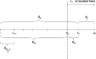
Figure 1: The construction of $\Pi_{0}$ for the Pólya tree prior.

Turning to the specification of $A_{0}$ for this partition $\Pi_{0}$, we propose the use of $\alpha_{\varepsilon}=\gamma_{m}H(B_{\varepsilon})$ in (4) with a base measure $H$ over $[0,\infty)$, which reflects available prior information. In our empirical example in Section 5.3, we illustrate the elicitation of such an $H$ based on an expert’s subjective judgments. We then consider the corresponding specification of $A_{0}$ using $\gamma_{m}=km^{2}$ with various values of $k$. In the absence of prior information, a seemingly reasonable default would be to let $H$ be a uniform distribution over $[0,y^{*}]$, where $y^{*}$ is the maximum possible valuation of the new product. For this $H,H(B_{\varepsilon})$ would be proportional to the length of $B_{\varepsilon}$, when $B_{\varepsilon}$ is bounded. Alternatively, the choice of a proper distribution $H$ with support $[0,\infty)$ would avoid the need to specify such a $y^{*}$ while still ensuring that $\alpha_{\varepsilon}=\gamma_{m}H(B_{\varepsilon})$ in (4) would be finite for any $B_{\varepsilon}$.

3.3.3 Updating the Pólya tree prior given second-price auction data

Letting $D$ denote our second-price auction data, we are now ready to describe how our Pólya tree prior $\operatorname{PT}(\Pi_{0},A_{0})$, with $\Pi_{0}$ in (3.3.2), can be conveniently updated to obtain the posterior Pólya tree distribution $\operatorname{PT}(\Pi_{0},A_{0}|D)$ for $F$. Recall that under the assumptions discussed in Section 2.2, each of the $M$ second-price auctions is associated with an i.i.d. sample of $N_{i}$ latent valuations $y_{iN_{i}}<\cdots<y_{i2}<y_{i1}$ from $F$. Of these, we only observe the second highest order statistics $y_{M2}<\cdots<y_{22}<y_{12}$ from each sample. The following update of $\operatorname{PT}(\Pi_{0},A_{0})$, based on just this information, is accomplished by exploiting the particular form of $\Pi_{0}$.

To begin with, the observed second highest bids $y_{M2}<\cdots<y_{22}<y_{12}$ by definition satisfy $y_{i2}\in[y_{i2},y_{(i-1)2})=B_{\underbrace{\mbox{{00\ldots 0}}}_{i-1}1}$, so that, for $i\geq 2$,

$$y_{i2}\in B_{\underbrace{\mbox{{00\ldots 0}}}_{i-1}1}\in B_{\underbrace{\mbox{{00\ldots 0}}}_{i-1}}\in\cdots\in B_{0},$$ (6)

a consequence of the nesting of the sets in $\Pi_{0}$. Next, although we do not observe $y_{i3},\ldots,y_{iN_{i}}$, we do know that $y_{i2}>y_{i3}>\cdots>y_{iN_{i}}$, so that $y_{i3},\ldots,\allowbreak y_{iN_{i}}\in(0,y_{i2})=B_{\underbrace{\mbox{{00\ldots 0}}}_{i}}$ and, again because of the nesting in $\Pi_{0}$,

$$y_{iN_{i}},y_{i(N_{i}-1)},\ldots,y_{i3}\in B_{\underbrace{\mbox{{00\ldots 0}}}_{i}}\in B_{\underbrace{\mbox{{00\ldots 0}}}_{i-1}}\in\cdots\in B_{0}.$$ (7)

Thus, to update the Pólya tree prior for all but the maximum valuations $y_{11},\allowbreak y_{21},\ldots,y_{M1}$, we simply increment the $A_{0}$ hyperparameter values via (3) as follows. For each auction $i$, we count one value $y_{i2}$ in each of $B_{0},B_{00},\ldots,\allowbreak B_{\underbrace{\mbox{{00\ldots 0}}}_{i-1}},B_{\underbrace{\mbox{{00\ldots 0}}}_{i-1}1}$ and $(N_{i}-2)$ values in each of $B_{0},B_{00},\ldots,B_{\underbrace{\mbox{{00\ldots 0}}}_{i}}$.

Beyond the updating above, the only values left to consider are the maximum valuations $y_{11},y_{21},\ldots,y_{M1}$. Except for $y_{11}$, which must be located in $[y_{12},\infty)=B_{1}$, there is uncertainty about the $B_{\varepsilon}$ location of these maximum values. For instance, consider $y_{21}$; as shown in Figure 1, given that $y_{21}>y_{22}$ by definition, we know that $y_{21}$ must be located in either $B_{01}$ or $B_{1}$, but we do not know which one. What we do know is that each $y_{i1}$ is located in some $B_{\varepsilon}$ where the binary index $\varepsilon$ consists of ($k-1$) $0$’s followed by a single 1 for some $k=1,\ldots,i$. To incorporate this partial information about the location of $y_{11},y_{21},\ldots,y_{M1}$ into the posterior update of $F$, we propose a Gibbs sampler similar to the algorithm proposed by Paddock (2002).

For $i=1,\ldots,M$, let $z_{i}\in\{1,\ldots,i\}$ where $z_{i}=k\Rightarrow y_{i1}\in B_{\underbrace{\mbox{{00\ldots 0}}}_{k-1}1}$ indicates the partition membership of $y_{i1}$. Thus, the remaining uncertainty about the update of $A_{0}$ concerns only the unknown values of $Z=(z_{1},z_{2},\ldots,z_{M})$. Indeed, together with the membership information in (6) and (7), the values of $Z$, if known, would yield the complete membership information indicated in Table 1. This information would then enable a complete update of $A_{0}$ via (3), which would in turn let us simulate a draw of $C_{\Pi}$, the set of $C_{\varepsilon 0}$’s corresponding to the partition $\Pi$.

Table 1: The number of observations in each partition, given $z_{i}$’s

Partition	Count	Partition	Count
$B_{0}$	$\sum_{i=1}^{M}(N_{i}-1)+\sum_{i=1}^{M}I\{z_{i}\geq 2\}-1$	$B_{1}$	$\sum_{i=1}^{M}I\{z_{i}=1\}+1$
$B_{00}$	$\sum_{i=2}^{M}(N_{i}-1)+\sum_{i=1}^{M}I\{z_{i}\geq 3\}-1$	$B_{01}$	$\sum_{i=1}^{M}I\{z_{i}=2\}+1$
$B_{\underbrace{\mbox{{00\ldots 0}}}_{k}}$	$\sum_{i=k}^{M}(N_{i}-1)+\sum_{i=1}^{M}I\{z_{i}\geq k+1\}-1$	$B_{\underbrace{\mbox{{00\ldots 0}}}_{k-1}1}$	$\sum_{i=1}^{M}I\{z_{i}=k\}+1$
$B_{\underbrace{\mbox{{00\ldots 0}}}_{M}}$	$(N_{M}-1)-1$	$B_{\underbrace{\mbox{{00\ldots 0}}}_{M-1}1}$	$\sum_{i=1}^{M}I\{z_{i}=M\}+1$

These observations provide the basis for the following Gibbs sampler updating scheme. First, we simulate $C_{\Pi}$ from $P(C_{\Pi}|A_{0},D,Z)$, where each $C_{\varepsilon 0}|\allowbreak A_{0},D,Z\sim\operatorname{Be}(\alpha_{\varepsilon 0}^{D,Z},\alpha_{\varepsilon 1}^{D,Z})$ is drawn independently based on the $(D,Z)$-updated values of $A_{0}$, namely, $(\alpha_{\varepsilon 0}^{D,Z},\alpha_{\varepsilon 1}^{D,Z})$. Second, conditionally on $C_{\Pi}$, the entries of $Z$ are conditionally independent. Thus, we simulate the unknown values of $Z$ from $P(Z|C_{\Pi})$ which are given by

$$P(z_{i}=1|C_{\Pi}) = P(y_{i1}\in B_{1}|C_{\Pi})=c_{i}C_{1},$$

$$P(z_{i}=2|C_{\Pi}) = P(y_{i1}\in B_{01}|C_{\Pi})=c_{i}C_{1}C_{01},$$

$$\vdots$$

$$P(z_{i}=i|C_{\Pi}) = P(y_{i1}\in B_{\underbrace{\mbox{{00\ldots 0}}}_{i-1}1}|C_{\Pi})=c_{i}C_{1}C_{01}\cdots C_{\underbrace{\mbox{{00\ldots 0}}}_{i-1}1},$$

where $c_{i}$ denotes the normalizing constant such that the above probabilities sum up to 1. This follows directly from (2) and the fact that normalization is needed to account for the membership restrictions on $y_{i1}$, because our auction data is sorted. By iteratively simulating from $P(C_{\Pi}|A_{0},D,Z)$ followed by $P(Z|C_{\Pi})$ in this manner, this Gibbs sampler can be used to simulate a sequence of $C_{\Pi}$ that is converging in distribution to $P(C_{\Pi}|A_{0},D)$, the posterior of $C_{\Pi}$ under $\operatorname{PT}(\Pi_{0},A_{0}|D)$.

3.3.4 Inference about $F$

It follows from (2) that under each realization of $C_{\Pi}$ from the Pólya tree posterior $\operatorname{PT}(\Pi_{0},A_{0}|D)$, the probability of a set $B_{\varepsilon_{1}\cdots\varepsilon_{m}}\in\Pi_{0}$ is given by

$$P(B_{\varepsilon_{1}\cdots\varepsilon_{m}}|A_{0},D)=\prod_{i=1}^{m}C_{\varepsilon_{1}\cdots\varepsilon_{i}}.$$ (9)

For the purpose of estimating these probabilities, and hence $F$, a natural estimate in this context is the posterior expectation of (9), namely,

$$E[P(B_{\varepsilon_{1}\cdots\varepsilon_{m}}|A_{0},D)]=E\Biggl{[}\prod_{i=1}^{m}C_{\varepsilon_{1}\cdots\varepsilon_{i}}|A_{0},D\Biggr{]},$$ (10)

which we can in turn estimate as follows. Based on a sequence of $T$ draws from the sequence of $C_{\Pi}$ from the Gibbs sampler (ignoring $s$ burn-in iterations), we estimate (10) by the Rao-Blackwellized version of $\frac{1}{T}\sum_{t=s}^{t=s+T}\prod_{i=1}^{m}C_{\varepsilon_{1}\cdots\varepsilon_{i}}^{(t)}$, namely,

$$\frac{1}{T}\sum_{t=s}^{t=s+T}\!E\Biggl{(}\prod_{i=1}^{m}\!C_{\varepsilon_{1}\cdots\varepsilon_{i}}^{(t)}|A_{0},D,Z^{(t)}\Biggr{)}\,{=}\,\frac{1}{T}\sum_{t=s}^{t=s+T}\prod_{i=1}^{m}\frac{\alpha_{\varepsilon_{1}\cdots\varepsilon_{i}}^{(t)}}{\alpha_{\varepsilon_{1}\cdots\varepsilon_{i-1}0}^{(t)}\,{+}\,\alpha_{\varepsilon_{1}\cdots\varepsilon_{i-1}1}^{(t)}},$$ (11)

where $\alpha_{\varepsilon_{1}\cdots\varepsilon_{i}}^{(t)}$ is the updated value of $\alpha_{\varepsilon_{1}\cdots\varepsilon_{i}}$ in $A_{0}$ based on $D$ and $Z^{(t)}$. This is our posterior estimate of $F$. The uncertainty of (11) as an estimate of (10), due to the unknown values of $Z=(z_{1},z_{2},\ldots,z_{M})$, can be summarized by suitable quantiles of the $T$ values of $\prod_{i=1}^{m}[\alpha_{\varepsilon_{1}\cdots\varepsilon_{i}}^{(t)}/(\alpha_{\varepsilon_{1}\cdots\varepsilon_{i-1}0}^{(t)}+\alpha_{\varepsilon_{1}\cdots\varepsilon_{i-1}1}^{(t)})]$ appearing in (10). Finally, the uncertainty of (11) as an estimate of (9) can be summarized by suitable quantiles of the corresponding $T$ values of $\prod_{i=1}^{m}C_{\varepsilon_{1}\cdots\varepsilon_{i}}^{(t)}$ from the Gibbs sequence.

4 Simulation study

In this section we compare the performance of our proposed Pólya tree method with Bayesian parametric approaches for estimating profit-maximizing prices. We consider parametric approaches based on the gamma and truncated-normal distributions, two parametric distributions commonly used in marketing research. For the posterior calculation with these parametric methods, we used a random-walk Metropolis–Hasting algorithm [Robert and Casella (2004)]. We also study the relationship between sample size and the accuracy of the estimators.

4.1 Data simulation

We conducted three sets of simulation experiments, each using data simulated from a different functional form for the underlying valuation distribution $F$. For the data from each $F$, we applied our Pólya tree approach and the two parametric Bayesian approaches, all using relatively noninfluential priors, to compute the profit-maximizing price and the corresponding expected profit. For the Pólya tree prior $\operatorname{PT}(\Pi_{0},A_{0})$ with partition $\Pi_{0}$ in (3.3.2), we set the hyperparameters $A_{0}$ using $\alpha_{\varepsilon}=km^{2}H(B_{\varepsilon})$ with $H$ uniform on $[0,y^{*}]$ as discussed in Section 3.3.2, with $m=m(\varepsilon)$ denoting the level (depth) of $B_{\varepsilon}$, and with $k$ set to a small but positive number $\delta(=e^{-20})$ in order to limit the $\alpha_{\varepsilon}$’s to being weakly informative. For the $\operatorname{gamma}(a,b)$ and truncated-normal($\mu,\sigma^{2}$) approaches we used the diffuse priors $a,b\sim\mbox{truncated-normal}(0,100^{2})$, $\mu\sim N(0,100^{2})$ and $\sigma\sim\mbox{truncated-normal}(0,100^{2})$.

We evaluate the performance of each method by the expected profit generated from their estimated profit-maximizing price. First, their profit maximizing price is obtained by maximizing an estimated expected (per-bidder) profit function based on the estimate $\hat{F}$ of $F$,

$$\hat{x}=\mathop{\arg\max}_{x}\hat{\pi}(x)=\mathop{\arg\max}_{x}\bigl{(}1-\hat{F}(x)\bigr{)}(x-c).$$

Their corresponding expected (per-bidder) profit is then obtained by plugging $\hat{x}$ into the actual (“true”) profit function:

$$\pi(\hat{x})=\bigl{(}1-F(\hat{x})\bigr{)}(\hat{x}-c).$$

In each case, the per-unit cost $c$ is taken to be $5.2 (the actual per-unit cost for the application in Section 5). Note that the (per-bidder) profit function is defined by multiplying the proportion of bidders who have a valuation higher than price $x$ [i.e., $1-F(x)$] and the profit for each sale $(x-c)$.

The density functions corresponding to the three underlying $F$ distributions we used are shown in Figure 2. For the first set of simulations, the underlying $F$ is a gamma distribution with shape

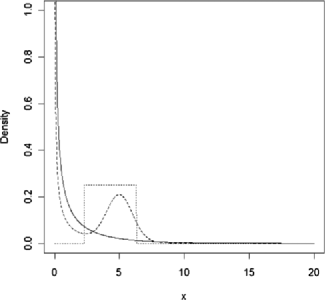
Figure 2: “True” underlying valuation distributions used in the simulation studies. Solid line: gamma$(0.32,0.26)$; broken line: equally weighted mixture of gamma$(0.32,0.26)$ and truncated-normal$(5.0,1.0)$; dotted line: uniform$(2.3,6.3)$.

parameter 0.32 and rate parameter 0.26 (values chosen to replicate features of the actual data in our empirical application in Section 5). For the second set of simulations, the underlying $F$ is an equally weighted mixture of the gamma$(0.32,0.26)$ and truncated-normal$(5.0,1.0)$ distributions. From a managerial perspective, this corresponds to a market with two distinct consumer segments with different average valuations. From a statistical perspective, this corresponds to a bimodal distribution for which both of our parameter approaches are misspecified. For the third set of simulations, the underlying $F$ is uniform$(2.3,6.3)$ (centered near the average observed transaction prices in our empirical application). This is similar to the distribution used in Jank and Zhang (2011).

From each of these three $F$’s, we simulated three data sets containing $M=1\mbox{,}000,100$ and 16 auctions (the number of auctions in our empirical application). Varying the sample size here sheds light on the relationship between the sample size and the precision of the optimal-price and expected profit estimates. For each auction, we simulated the number of bidders from a Poisson distribution with mean 18.5 (the average number of bidders in our empirical application). We then drew the bidders’ valuations from $F$, keeping only the second highest. To account for sample-to-sample variation, we repeated the $M=1\mbox{,}000$ case 10 times, and the $M=100$ and $M=16$ cases 100 times, reporting the standard errors along with the mean.

Table 2: Simulation results. The standard errors are shown in brackets

	Pólya tree		Gamma		Truncated-normal
		Profit		Profit		Profit
	Price	($0.01/bidder)	Price	($0.01/bidder)	Price	($0.01/bidder)
(a) For $\operatorname{gamma}(0.32,0.27)$ distribution
$M=1\mbox{,}000$	8.45	6.25	8.38	6.36	6.57	4.92
	(0.22)	(0.04)	(0.02)	(0.00)	(0.01)	(0.01)
$M=100$	9.13	5.72	8.29	6.33	6.54	4.86
	(0.23)	(0.10)	(0.03)	(0.00)	(0.01)	(0.01)
$M=16$	8.77	5.45	8.18	6.16	6.54	4.83
	(0.23)	(0.11)	(0.08)	(0.02)	(0.02)	(0.03)
(b) For equally weighted mixture between $\operatorname{gamma}(0.32,0.27)$ and truncated-normal$(5.0,1.0)$
$M=1\mbox{,}000$	5.97	8.05	6.45	6.94	6.15	7.89
	(0.02)	(0.01)	(0.01)	(0.03)	(0.02)	(0.04)
$M=100$	6.20	7.85	6.40	7.12	6.16	7.79
	(0.13)	(0.09)	(0.01)	(0.03)	(0.02)	(0.04)
$M=16$	6.49	7.16	6.41	7.04	6.29	7.19
	(0.15)	(0.15)	(0.02)	(0.06)	(0.04)	(0.12)
(c) For uniform$(2.3,6.3)$ distribution
$M=1\mbox{,}000$	5.77	7.53	6.31	0.13	5.68	7.43
	(0.01)	(0.01)	(0.01)	(0.08)	(0.00)	(0.01)
$M=100$	5.76	7.43	6.22	2.09	5.68	7.39
	(0.01)	(0.02)	(0.00)	(0.09)	(0.00)	(0.01)
$M=16$	5.78	7.14	6.26	1.61	5.76	6.94
	(0.01)	(0.06)	(0.01)	(0.17)	(0.03)	(0.16)

4.2 Simulation results

A key feature of our Pólya tree approach is robust estimation of the profit-maximizing price in the sense that, compared to parametric methods, it is less sensitive to a misspecified form for the consumer valuation distribution $F$. Although we would not expect it to perform as well as a correctly prespecified parametric method, we would like it to perform better than an incorrectly prespecified parametric method. Such performance is precisely borne out by our first simulation where the true $F$ was a gamma distribution. As shown in Table 2(a), the best performance was obtained by the gamma parametric approach, for which the estimated profit-maximizing price was closest to the true value, leading to the highest expected profit. As expected, the Pólya tree approach performed slightly worse than the “correctly specified” gamma parametric method but substantially better than the “incorrectly specified” truncated-normal distribution method.

=260pt Pólya tree Gamma Trunc-normal (a) $M=1\mbox{,}000$ True: gamma $-1.7\%$ $0.0\%$ $-22.6\%$ True: mixture $-0.4\%$ $-14.1\%$ $-2.4\%$ True: uniform $-0.4\%$ $-98.3\%$ $-1.7\%$ (b) $M=100$ True: gamma $-10.1\%$ $-0.5\%$ $-23.6\%$ True: mixture $-2.8\%$ $-11.9\%$ $-3.6\%$ True: uniform $-1.7\%$ $-72.4\%$ $-2.2\%$ (c) $M=16$ True: gamma $-14.3\%$ $-3.1\%$ $-24.1\%$ True: mixture $-11.4\%$ $-12.9\%$ $-11.0\%$ True: uniform $-5.6\%$ $-78.7\%$ $-8.2\%$

Table 3: Performance of each method (PT, gamma, truncated-normal) compared to the profit under optimal price

Turning to the second simulation in Table 2(b), where the true $F$ was an equally-weighted mixture of gamma and truncated-normal distributions, the Pólya tree method performed best in every case except one, where the size of auctions $M=16$ was small and the truncated-normal approach performed slightly better. Finally, for the third simulation in Table 2(c), when the true $F$ was a uniform distribution, the Pólya tree method clearly outperformed both parametric approaches, a situation where the performance of the gamma approach was particularly bad. Taken together, the three simulations illustrate how, in contrast to the robustness of the Pólya tree approach, the parametric approaches can perform poorly when the parametric form is misspecified.

Table 3(a)–(c) summarizes the results in Table 2(a)–(c) by comparing the percentage profit loss (compared to the profit under optimal price), for each method, across the different values of $M$. As can be seen in Table 3(a)–(c), the performance of the Pólya tree method is more robust compared to other methods, in the sense that it offers the best worst-case performance, a minimax kind of appeal. By avoiding the need for a prespecified functional form, the Pólya tree method avoids the potentially poor performance due to misspecfication (e.g., using the parametric gamma method in the third simulation). Finally, with respect to sample size and estimation accuracy, we note that the estimation accuracy of all the methods deteriorates with smaller sample sizes $M$. The results in Tables 2 and 3 further suggest that if the number of auctions $M$ is very small (16), it may be helpful to introduce managerial knowledge through a prior distribution on the valuation distribution. For that purpose, the Pólya tree approach offers the flexibility of being able to incorporate prior knowledge by centering the Pólya tree prior around any base measure $H$, whereas for parametric methods, prior knowledge is restricted to prior distributions over the parameters of a particular form.

5 Empirical application

In this section we apply our method to estimate the profit-maximizing price of a new jewelry product based on actual data obtained from second-price auction experiments. In Section 5.1 we describe the experiments and provide an overview of the data. In Section 5.2 we apply and compare our Pólya tree approach with parametric approaches based on the gamma and truncated-normal distributions. In Section 5.3 we take a step further to illustrate the incorporation into our estimation procedure of a manager’s elicited prior beliefs about the consumer valuation distribution.

5.1 Data overview

In collaboration with an online jewelry retailer, a total of $M=16$ identical, nonoverlapping, second-price auction experiments were conducted on a major internet auction site from February 25, 2006 to March 20, 2006. Each auction lasted 24 hours, starting and ending at midnight. The transaction price of the completed auction was recorded and adjusted for the small increment to obtain the bidders’ second highest valuation $y_{i2}$. Using third-party tracking software, the jeweler also recorded the total number of unique users who viewed each auction (i.e., the total number of bidders). The sorted data are shown in Table 4. To increase the chance of observing some bidding

Table 4: Sorted data from the sixteen online second-price auction experiments

$N_{i}$	25	12	22	21	20	27	19	13
$y_{i2}$	10.05	8.50	5.51	5.50	5.49	5.12	4.69	4.25
$N_{i}$	19	12	17	22	14	13	25	16
$y_{i2}$	3.73	3.53	3.25	2.34	2.26	2.02	1.50	1.25

activity in each auction, the starting price was always set to $0.01 with free shipping. As it turned out, each auction had at least twelve bidders, so that the second-highest bid was indeed observed in each auction. For the jewelry product we considered, the per-unit cost $c$ was constant and equal to $5.20.

5.2 Posterior inference for the valuation distribution in the absence of prior information

For the case where prior information was unavailable, we applied the methods considered in Section 4, namely, our proposed Pólya tree method and the gamma and truncated-normal parametric Bayesian methods with the weakly informative prior distributions, to the auction data in Table 4. For the Pólya tree method, we used the partition $\Pi_{0}$

=285pt Prior probability Partition Interval $\bolds{p_{\varepsilon}=H(B_{\varepsilon})}$ $B_{0}$ 1(0.00, 10.05) 0.901 $B_{1}$ [10.05, $\infty)$00. 0.099 $B_{00}$ (0.00, 8.50) 0.870 $B_{01}$ 0[8.50, 10.05) 0.031 $B_{000}$ (0.00, 5.51) 0.731 $B_{001}$ [5.51, 8.50) 0.139 $B_{0000}$ (0.00, 5.50) 0.730 $B_{0001}$ [5.50, 5.51) 0.001 $B_{00000}$ (0.00, 5.49) 0.729 $B_{00001}$ [5.49, 5.50) 0.001 $B_{000000}$ (0.00, 5.12) 0.707 $B_{000001}$ [5.12, 5.49) 0.022 $B_{0000000}$ (0.00, 4.69) 0.685 $B_{0000001}$ [4.69, 5.12) 0.023 $B_{00000000}$ (0.00, 4.25) 0.663 $B_{00000001}$ [4.25, 4.69) 0.022 $B_{000000000}$ (0.00, 3.73) 0.637 $B_{000000001}$ [3.73, 4.25) 0.026 $B_{0000000000}$ (0.00, 3.53) 0.627 $B_{0000000001}$ [3.53, 3.73) 0.010 $B_{00000000000}$ (0.00, 3.25) 0.613 $B_{00000000001}$ [3.25, 3.53) 0.014 $B_{000000000000}$ (0.00, 2.34) 0.534 $B_{000000000001}$ [2.34, 3.25) 0.079 $B_{0000000000000}$ (0.00, 2.26) 0.526 $B_{0000000000001}$ [2.26, 2.34) 0.008 $B_{00000000000000}$ (0.00, 2.02) 0.502 $B_{00000000000001}$ [2.02, 2.26) 0.024 $B_{000000000000000}$ (0.00, 1.50) 0.450 $B_{000000000000001}$ [1.50, 2.02) 0.052 $B_{0000000000000000}$ (0.00, 1.25) 0.425 $B_{0000000000000001}$ [1.25, 1.50) 0.025

Table 5: First two columns: the partition scheme $\Pi_{0}$ used in the empirical application. The third column is used to set $A_{0}$ to approximate the manager’s prior beliefs

in (3.3.2), given by the first two columns of Table 5. Notice how the partition elements only split on the leftmost set at each level.

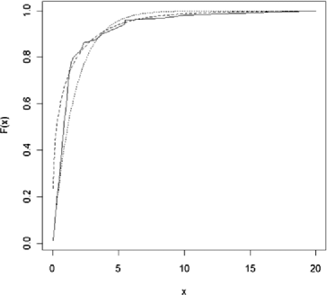
Figure 3: Estimates of the valuation distributions $F$ by the three different methods: Pólya tree (solid line); gamma (broken line); truncated-normal (dotted line).

The estimates of the valuation distribution $F$ for each method are shown in Figure 3, and the estimated profit functions (along with the estimated optimal prices for each method) are shown in Figure 4. We see that while the overall shapes of the valuation distributions are quite similar across all three methods, the quantiles of the three distributions differ widely. For instance, the median valuation is $0.85 for the Pólya tree method, $0.29 for the gamma method and $1.13 for the truncated-normal method. Thus, the resulting inference of the optimal price is similarly highly sensitive to the particular assumption made for the functional form. The estimated optimal price using the Pólya tree method is $12.6, while the estimated optimal prices from gamma and truncated-normal parametric methods are $8.63 and $6.69, respectively.

5.3 Incorporating elicited managerial prior beliefs

As discussed early, an appealing additional feature of the Bayesian Pólya tree method is how prior beliefs about $F$ can be straightforwardly incorporated into the Pólya tree prior $\operatorname{PT}(\Pi_{0},A_{0})$. We illustrate this here with the construction of a prior that incorporates an expert’s beliefs about the valuation distribution $F$ of potential consumers for the auctioned jewelry product. It is worth noting that it is not clear how to incorporate the elicited beliefs described below into the parametric priors that we have been discussing.

In an interview with the manager of the online jewelry retailer behind our auctions, we used the following subjective CDF construction method [Berger (1985), page 81] to elicit his prior belief about $F$. Asking him to imagine a hypothetical random sample of 100 consumers, the manager was asked to state X for various Y values in the following statement: “If the price is set at Y dollars, X (out of 100) consumers are willing to buy the product.” Table 6 shows the set of the manager’s responses [i.e., (X,Y) pairs]. By joining these points with linear segments, these responses were converted into a cdf, which we denote by $H$.

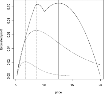
Figure 4: Estimated profit functions for the Pólya tree method (solid line), gamma (broken line); truncated-normal (dotted line).

=260pt $\bolds{\ldots}$X (out of 100) consumers are If the price is set at $Y$\bolds{\ldots}$ willing to buy the jewelry product $0.01$ $98$ $0.50$ $70$ $1.00$ $60$ $2.00$ $50$ $3.00$ $40$ $5.00$ $30$ $7.50$ $15$ $10.00$ $10$ $12.00$ $7$ $14.00$ $6$ $15.00$ $2$ $20.00$ $0$

Table 6: Manager’s prior beliefs about the consumer valuation distribution

Again using the partition $\Pi_{0}$ in Table 5, we proceeded to set $A_{0}$ so that the prior $\operatorname{PT}(\Pi_{0},A_{0})$ approximates the manager’s prior beliefs. For this purpose, we set $\alpha_{\varepsilon}=km^{2}p_{\varepsilon}$, the special case of $\alpha_{\varepsilon}=\gamma_{m}H(B_{\varepsilon})$ discussed in Section 3.3.2 with $p_{\varepsilon}=H(B_{\varepsilon})$ and $m$ the level of $B_{\varepsilon}$. This setting serves to center the prior at prior probabilities $p_{\varepsilon}=H(B_{\varepsilon})$, shown in the third column of Table 5, which match the manager’s prior $H$. For $k$, we considered various values $k=\delta,10,20,50$, to gauge the effects of different levels of prior uncertainty on the posterior for $F$. Larger $k$ reflects a more certain prior assessment of $F$, yielding a posterior distribution that is less influenced by the observed data.

For the prior $\operatorname{PT}(\Pi_{0},A_{0})$ choices described above, we estimated the profit-maximizing price. Figure 5 shows the various estimated valuation distributions which incorporate the manager’s prior beliefs. The resulting posterior estimates are shown for the four values of $k\dvtx\delta$ (top broken line), 10 (second broken line), 20 (third broken line), and 50 (bottom broken line), along with the manager’s prior beliefs about $F$ (solid line). These results provide a number of insights. First, as can be seen in the figure, all the posterior estimates of $F$ are above the prior $H$, suggesting that consumers here have a stochastically lower valuation of the product than that suggested by the manager’s prior beliefs. Second, we observe that with smaller values of $k$, as expected, the posterior estimate is more influenced by the second-price auction data and less influenced by the prior.

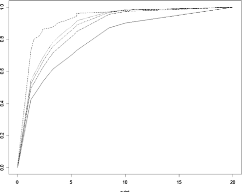
Figure 5: Posterior estimates of the consumer valuation distribution $F$. The solid line is the manager’s prior belief; the other four lines represent, from top to bottom, the posterior estimates for the four values $k=\delta,10,20,50$, respectively.

Next, we turn to estimating the profit-maximizing price for each value of $k$. The profit function for each value of $k$, along with the estimated profit maximizing price, is shown in Figure 6. Figure 6 offers some insights about two potential pricing strategies. There are two price points (around $7.50 and $12.60), that roughly correspond to two pricing strategies commonly used in new product pricing [e.g., Tellis (1986)]: (i) a “skimming” strategy that targets only a high-value consumer segment (hence achieving very low volume, but high profit per transaction), and (ii) a “penetration” strategy where the retailer sets the price lower in order to achiever a higher initial penetration, but a lower profit-per-transaction. The relative effectiveness of each strategy depends on the value of $k$, that is, the amount of weight that the manager puts on his prior belief.

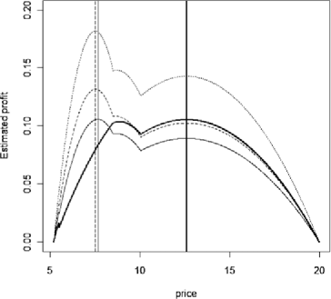
Figure 6: Estimated profit functions for the Pólya tree method after incorporating managerial prior knowledge; $k=\delta$ (thick solid line), $k=10$ (thin solid line); $k=20$ (broken line); $k=50$ (dotted line).

The estimated profit maximizing prices are $12.6, $7.66, $7.52 and $7.50 for $k=\delta,10,20,50$, respectively. We find that for $k<4$, a skimming strategy is more attractive; for $k>4$, a penetration strategy gives better profits. Thus, our method allows the retailer to quantify and compare the effectiveness of skimming vs. penetration strategies at any given $k$. Note also that somewhat counter-intuitively, a stochastically higher valuation distribution (using larger $k$) here leads to a lower optimal price. Although at each price a larger percentage of customers will buy the product, the effect of this on profits is more pronounced at the lower prices.

As can be seen in Figure 6, it appears that by incorporating some degree of prior managerial knowledge, the optimal price is estimated to be around $7.50. This can be used as a starting point for pricing the new jewelry product. Based on our recommendations, the jeweler implemented a fixed price of $7.49 when the new jewelry product was brought into market in late 2006.

Our method allows us to not only estimate the profit-maximizing price, but also to quantify the uncertainty for estimated profits under the optimal price, by using the posterior sample draws from the Pólya tree. Figure 7 displays the pointwise 90% posterior intervals for the profit function when $k=20$, which reflects the degree of uncertainty for our results. For example, the estimated profit (for the $k=20$ case) at the optimal price of $7.48 is $0.14 per bidder, with a 90% posterior interval of ($0.09, $0.18). This provides the retailer with an estimate of the range of profit that can be obtained.

6 Discussion and future research

In this paper we have developed a nonparametric Bayesian methodology that enables retailers to estimate the optimal price for a new product by learning about the consumer valuation distribution from second-price auction data. Using a flexible Pólya tree distribution to represent uncertainty about the unknown consumer valuation distribution, we have proposed a Pólya tree prior formulation and computational approach that allows for fast updating of the hyperparameters using only second highest order statistics obtained from a set of auctions. Through collaboration with an online jewelry retailer, we apply our methodology to incorporate managerial prior beliefs and derive the optimal price for a new jewelry product. The generality of our proposed methodology allows for its application to many different products.

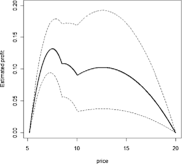
Figure 7: Pointwise 90% posterior intervals of the profit function ($k=20$ case).

A key to the computational advantages of our setup is the use of the observed second order statistics as the cutpoints for the prior partition $\Pi_{0}$ in (3.3.2). Although strict Bayesian coherence is violated by the use of the data to formulate the prior partition, it does not seem that the injected structural information is creating a particular bias. Nonetheless, because the Pólya tree posterior may still be influenced by $\Pi_{0}$ in addition to $A_{0}$, it is important to be mindful of the impact of some of its basic characteristics. While Pólya tree generalizations involving random partitions [e.g., Paddock et al. (2003), Wong and Ma (2010)] would be a way to mitigate this influence, the computational burdens of their implementation would likely be overwhelming for the second-price auction data.

One aspect of $\Pi_{0}$ that does appear to incur some systematic bias is the assignment of the $y_{i2}$’s to the upper intervals (e.g., $y_{12}\in B_{1};y_{22}\in B_{01}$, etc.) by defining the upper intervals $B_{\varepsilon 1}$ in (3.3.2) to be left closed. However, the upward bias resulting from posterior updating with this upper interval assignment is substantially smaller than the downward bias that would result from a lower interval assignment (details available upon request). Another alternative, left for future research, might be to consider partial probabilistic assignments of each of the $y_{i2}$’s to both intervals.

Finally, the choice of the left telescoping hierarchy does also influence the posterior. As illustrated in Web Appendix I [George and Hui (2011)], this influence of the chosen hierarchy is lessened when $\alpha_{\varepsilon}=\gamma_{m}H(B_{\varepsilon})$ with $\gamma_{m}$ chosen very small, so that $\gamma_{m}$ is approximately constant, at least at the lower levels. However, this strategy would be inappropriate for the scenario in Section 5.3, where we would not want to minimize the impact of an informative managerial prior. Due to the level dependent weighting of the prior through $m^{2}$, the intervals at the deeper levels have a stronger prior, resulting in a posterior that will be sensitive to the choice of hierarchy. In future work, it may be useful to consider alternative hierarchies that may better represent the manager’s prior beliefs and uncertainty about them. We leave the issue of eliciting the most reasonable hierarchy and associated level-dependent weighting function as a future research direction.

To conclude, our research adds to the recent and growing stream of literature on the use of Bayesian nonparametric techniques in marketing [e.g., Braun et al. (2006), Brezger and Steiner (2008), Kim, Menzefricke and Feinberg (2004, 2007), Sood, James and Tellis (2009)]. Bayesian nonparametric techniques provide a rich toolkit that allows modelers to avoid imposing restrictive parametric functional forms. Braun et al. (2006) and Kim, Menzefricke and Feinberg (2004) utilize a Dirichlet process prior to specify the heterogeneity distribution; Brezger and Steiner (2008) and Kim, Menzefricke and Feinberg (2007) use a Bayesian spline approach to model the price response function. In the same spirit, this paper introduces the Pólya tree prior to model uncertainty about an unknown consumer valuation distribution for the purpose of optimal price estimation. To the best of our knowledge, this is the first marketing application to make use of a Pólya tree distribution; we certainly hope that in the future, this flexible class of distributions will be added to the modeler’s toolkit.

References

- Adams (2007) {barticle}[auto:STB—2011/09/12—07:03:23] \bauthor\bsnmAdams, \bfnmChristopher P.\binitsC. P. (\byear2007). \btitleEstimating Demand from eBay prices. \bjournalInternational Journal of Industrial Organization \bvolume25 \bpages1213–1232. \bptokimsref \endbibitem
- Baldwin, Marshall and Richard (1997) {barticle}[auto:STB—2011/09/12—07:03:23] \bauthor\bsnmBaldwin, \bfnmLaura H.\binitsL. H., \bauthor\bsnmMarshall, \bfnmRobert C.\binitsR. C. and \bauthor\bsnmRichard, \bfnmJean-Francois\binitsJ.-F. (\byear1997). \btitleBidder collusion at forest timber sales. \bjournalJournal of Political Economy \bvolume105 \bpages657–699. \bptokimsref \endbibitem
- Bapna et al. (2009) {barticle}[auto:STB—2011/09/12—07:03:23] \bauthor\bsnmBapna, \bfnmR.\binitsR., \bauthor\bsnmChang, \bfnmS. A.\binitsS. A., \bauthor\bsnmGoes, \bfnmP.\binitsP. and \bauthor\bsnmGupta, \bfnmA.\binitsA. (\byear2009). \btitleOverlapping online auctions: Empirical characterization of bidder strategies and auction prices. \bjournalMIS Quarterly \bvolume33 \bpages763–783. \bptokimsref \endbibitem
- Berger (1985) {bbook}[mr] \bauthor\bsnmBerger, \bfnmJames O.\binitsJ. O. (\byear1985). \btitleStatistical Decision Theory and Bayesian Analysis, \bedition2nd ed. \bpublisherSpringer, \baddressNew York. \bidmr=0804611 \bptokimsref \endbibitem
- Boatwright, Borle and Kadane (2010) {barticle}[auto:STB—2011/09/12—07:03:23] \bauthor\bsnmBoatwright, \bfnmPeter\binitsP., \bauthor\bsnmBorle, \bfnmSharad\binitsS. and \bauthor\bsnmKadane, \bfnmJoseph B.\binitsJ. B. (\byear2010). \btitleCommon value vs. private value categories in online auctions: A distinction without a difference? \bjournalDecision Analysis \bvolume7 \bpages86–98. \bptokimsref \endbibitem
- Bradlow and Park (2007) {barticle}[auto:STB—2011/09/12—07:03:23] \bauthor\bsnmBradlow, \bfnmEric T.\binitsE. T. and \bauthor\bsnmPark, \bfnmYoung Hoon\binitsY. H. (\byear2007). \btitleBayesian estimation of bid sequences in internet auctions using a generalized record-breaking model. \bjournalMarketing Science \bvolume26 \bpages218–229. \bptokimsref \endbibitem
- Braun et al. (2006) {barticle}[auto:STB—2011/09/12—07:03:23] \bauthor\bsnmBraun, \bfnmMichael\binitsM., \bauthor\bsnmFader, \bfnmPeter S.\binitsP. S., \bauthor\bsnmBradlow, \bfnmEric T.\binitsE. T. and \bauthor\bsnmKunreuther, \bfnmHoward\binitsH. (\byear2006). \btitleModeling the “Pseudodeductible” in insurance claims decision. \bjournalManagement Science \bvolume52 \bpages1258–1272. \bptokimsref \endbibitem
- Breidert (2006) {bmisc}[auto:STB—2011/09/12—07:03:23] \bauthor\bsnmBreidert, \bfnmChristoph\binitsC. (\byear2006). \bhowpublishedEstimation of willingness-to-pay: Theory, measurement, application, DUV. \bptokimsref \endbibitem
- Brezger and Steiner (2008) {barticle}[mr] \bauthor\bsnmBrezger, \bfnmAndreas\binitsA. and \bauthor\bsnmSteiner, \bfnmWinfried J.\binitsW. J. (\byear2008). \btitleMonotonic regression based on Bayesian P-splines: An application to estimating price response functions from store-level scanner data. \bjournalJ. Bus. Econom. Statist. \bvolume26 \bpages90–104. \biddoi=10.1198/073500107000000223, issn=0735-0015, mr=2422064 \bptokimsref \endbibitem
- Canals-Cerda and Pearcy (2010) {bmisc}[auto:STB—2011/09/12—07:03:23] \bauthor\bsnmCanals-Cerda, \bfnmJose\binitsJ. and \bauthor\bsnmPearcy, \bfnmJason\binitsJ. (\byear2010). \bhowpublishedArriving in time: Estimation of english auctions with a stochastic number of bidders. Working paper. Available at http:// papers.ssrn.com/sol3/papers.cfm?abstract_id=947605&download=yes. \bptokimsref \endbibitem
- Casella and Berger (2001) {bbook}[auto:STB—2011/09/12—07:03:23] \bauthor\bsnmCasella, \bfnmGeorge\binitsG. and \bauthor\bsnmBerger, \bfnmRoger L.\binitsR. L. (\byear2001). \btitleStatistical Inference, \bedition2nd ed. \bpublisherDuxbury, \baddressPacific Grove, CA. \bptokimsref \endbibitem
- Chakravarti et al. (2002) {barticle}[auto:STB—2011/09/12—07:03:23] \bauthor\bsnmChakravarti, \bfnmD.\binitsD., \bauthor\bsnmGreenleaf, \bfnmE.\binitsE., \bauthor\bsnmSinha, \bfnmA.\binitsA., \bauthor\bsnmCheema, \bfnmA.\binitsA., \bauthor\bsnmBox, \bfnmJ. C.\binitsJ. C., \bauthor\bsnmFriedman, \bfnmD.\binitsD., \bauthor\bsnmHo, \bfnmT. H.\binitsT. H., \bauthor\bsnmIssac, \bfnmR. M.\binitsR. M., \bauthor\bsnmMitchell, \bfnmA. A.\binitsA. A., \bauthor\bsnmRapoport, \bfnmA.\binitsA., \bauthor\bsnmRothkopf, \bfnmM. H.\binitsM. H., \bauthor\bsnmSrivastava, \bfnmJ.\binitsJ. and \bauthor\bsnmZwick, \bfnmR.\binitsR. (\byear2002). \btitleAuctions: Research opportunities in marketing. \bjournalMarketing Letters \bvolume13 \bpages281–296. \bptokimsref \endbibitem
- Chan, Kadiyali and Park (2007) {barticle}[auto:STB—2011/09/12—07:03:23] \bauthor\bsnmChan, \bfnmTat Y.\binitsT. Y., \bauthor\bsnmKadiyali, \bfnmVrinda\binitsV. and \bauthor\bsnmPark, \bfnmYoung-Hoon\binitsY.-H. (\byear2007). \btitleWillingness to pay and competition in online auctions. \bjournalJournal of Marketing Research \bvolume44 \bpages324–333. \bptokimsref \endbibitem
- Dey, Müller and Sinha (1998) {bbook}[mr] \beditor\bsnmDey, \bfnmDipak\binitsD., \beditor\bsnmMüller, \bfnmPeter\binitsP. and \beditor\bsnmSinha, \bfnmDebajyoti\binitsD., eds. (\byear1998). \btitlePractical Nonparametric and Semiparametric Bayesian Statistics. \bseriesLecture Notes in Statistics \bvolume133. \bpublisherSpringer, \baddressNew York. \bidmr=1630072 \bptokimsref \endbibitem
- Ferguson (1974) {barticle}[mr] \bauthor\bsnmFerguson, \bfnmThomas S.\binitsT. S. (\byear1974). \btitlePrior distributions on spaces of probability measures. \bjournalAnn. Statist. \bvolume2 \bpages615–629. \bidissn=0090-5364, mr=0438568 \bptokimsref \endbibitem
- George and Hui (2011) {bmisc}[auto:STB—2011/09/12—07:03:23] \bauthor\bsnmGeorge, \bfnmEdward\binitsE. and \bauthor\bsnmHui, \bfnmSam\binitsS. (\byear2011). \bhowpublishedSupplement to “Optimal pricing using online auction experiments: A Pólya tree approach.” DOI:10.1214/11-AOAS503SUPP. \bptokimsref \endbibitem
- Green and Srinivasan (1978) {barticle}[auto:STB—2011/09/12—07:03:23] \bauthor\bsnmGreen, \bfnmP. E.\binitsP. E. and \bauthor\bsnmSrinivasan, \bfnmV.\binitsV. (\byear1978). \btitleConjoint analysis in consumer research: Issues and outlook. \bjournalJournal of Consumer Research \bvolume5 \bpages103–123. \bptokimsref \endbibitem
- Haruvy et al. (2008) {barticle}[auto:STB—2011/09/12—07:03:23] \bauthor\bsnmHaruvy, \bfnmErnan\binitsE., \bauthor\bsnmLeszczyc, \bfnmPeter\binitsP., \bauthor\bsnmCarare, \bfnmOctavian\binitsO., \bauthor\bsnmCox, \bfnmJames C.\binitsJ. C., \bauthor\bsnmGreenleaf, \bfnmEric A.\binitsE. A., \bauthor\bsnmJank, \bfnmWolfgang\binitsW., \bauthor\bsnmJap, \bfnmSandy\binitsS., \bauthor\bsnmPark, \bfnmYoung-Hoon\binitsY.-H. and \bauthor\bsnmRothkopf, \bfnmMichael H.\binitsM. H. (\byear2008). \btitleCompetition between auctions. \bjournalMarketing Letters \bvolume19 \bpages431–448. \bptokimsref \endbibitem
- Hou and Rego (2007) {barticle}[auto:STB—2011/09/12—07:03:23] \bauthor\bsnmHou, \bfnmJianwei\binitsJ. and \bauthor\bsnmRego, \bfnmCesar\binitsC. (\byear2007). \btitleA classification of online bidders in a private value auction: Evidence from eBay. \bjournalInternational Journal of Electronic Marketing and Retailing \bvolume1 \bpages322–338. \bptokimsref \endbibitem
- Houser and Wooders (2006) {barticle}[auto:STB—2011/09/12—07:03:23] \bauthor\bsnmHouser, \bfnmDaniel\binitsD. and \bauthor\bsnmWooders, \bfnmJohn\binitsJ. (\byear2006). \btitleReputation in auctions: Theory, and evidence from eBay. \bjournalJournal of Economics and Management Strategy \bvolume15 \bpages353–369. \bptokimsref \endbibitem
- Jank and Zhang (2011) {barticle}[auto:STB—2011/09/12—07:03:23] \bauthor\bsnmJank, \bfnmW.\binitsW. and \bauthor\bsnmZhang, \bfnmS.\binitsS. (\byear2011). \btitleAn automated and data-driven bidding strategy for online auctions. \bjournalInforms J. Comput. \bvolume23 \bpages238–253. \bptokimsref \endbibitem
- Kim, Menzefricke and Feinberg (2004) {barticle}[auto:STB—2011/09/12—07:03:23] \bauthor\bsnmKim, \bfnmJin Gyo\binitsJ. G., \bauthor\bsnmMenzefricke, \bfnmUlrich\binitsU. and \bauthor\bsnmFeinberg, \bfnmFred\binitsF. (\byear2004). \btitleAssessing heterogeneity in discrete choice models using a Dirichlet process prior. \bjournalReview of Marketing Science \bvolume2 \bpages1–39. \bptokimsref \endbibitem
- Kim, Menzefricke and Feinberg (2007) {barticle}[auto:STB—2011/09/12—07:03:23] \bauthor\bsnmKim, \bfnmJin Gyo\binitsJ. G., \bauthor\bsnmMenzefricke, \bfnmUlrich\binitsU. and \bauthor\bsnmFeinberg, \bfnmFred\binitsF. (\byear2007). \btitleCapturing flexible heterogeneous utility curves: A Bayesian spline approach. \bjournalManagement Science \bvolume53 \bpages340–354. \bptokimsref \endbibitem
- Klemperer (1999) {barticle}[auto:STB—2011/09/12—07:03:23] \bauthor\bsnmKlemperer, \bfnmPaul\binitsP. (\byear1999). \btitleAuction theory: A guide to the literature. \bjournalJournal of Economic Surveys \bvolume13 \bpages227–286. \bptokimsref \endbibitem
- Laffont and Vuong (1996) {barticle}[auto:STB—2011/09/12—07:03:23] \bauthor\bsnmLaffont, \bfnmJean-Jacques\binitsJ.-J. and \bauthor\bsnmVuong, \bfnmQuang\binitsQ. (\byear1996). \btitleStructural analysis of auction data. \bjournalAmerican Economic Review \bvolume86 \bpages414–420. \bptokimsref \endbibitem
- Lavine (1992) {barticle}[mr] \bauthor\bsnmLavine, \bfnmMichael\binitsM. (\byear1992). \btitleSome aspects of Pólya tree distributions for statistical modelling. \bjournalAnn. Statist. \bvolume20 \bpages1222–1235. \biddoi=10.1214/aos/1176348767, issn=0090-5364, mr=1186248 \bptokimsref \endbibitem
- Lavine (1994) {barticle}[mr] \bauthor\bsnmLavine, \bfnmMichael\binitsM. (\byear1994). \btitleMore aspects of Pólya tree distributions for statistical modelling. \bjournalAnn. Statist. \bvolume22 \bpages1161–1176. \biddoi=10.1214/aos/1176325623, issn=0090-5364, mr=1311970 \bptokimsref \endbibitem
- Mauldin, Sudderth and Williams (1992) {barticle}[mr] \bauthor\bsnmMauldin, \bfnmR. Daniel\binitsR. D., \bauthor\bsnmSudderth, \bfnmWilliam D.\binitsW. D. and \bauthor\bsnmWilliams, \bfnmS. C.\binitsS. C. (\byear1992). \btitlePólya trees and random distributions. \bjournalAnn. Statist. \bvolume20 \bpages1203–1221. \biddoi=10.1214/aos/1176348766, issn=0090-5364, mr=1186247 \bptokimsref \endbibitem
- Mitchell and Carson (1989) {bmisc}[auto:STB—2011/09/12—07:03:23] \bauthor\bsnmMitchell, \bfnmRobert Cameron\binitsR. C. and \bauthor\bsnmCarson, \bfnmRichard T.\binitsR. T. (\byear1989). \bhowpublishedUsing Surveys to Value Public Goods: The Contingent Valuation Method. RFF Press, Washington, DC. \bptokimsref \endbibitem
- Muliere and Walker (1997) {barticle}[mr] \bauthor\bsnmMuliere, \bfnmPietro\binitsP. and \bauthor\bsnmWalker, \bfnmStephen\binitsS. (\byear1997). \btitleA Bayesian non-parametric approach to survival analysis using Polya trees. \bjournalScand. J. Statist. \bvolume24 \bpages331–340. \biddoi=10.1111/1467-9469.00067, issn=0303-6898, mr=1481419 \bptokimsref \endbibitem
- Ockenfels and Roth (2006) {barticle}[mr] \bauthor\bsnmOckenfels, \bfnmAxel\binitsA. and \bauthor\bsnmRoth, \bfnmAlvin E.\binitsA. E. (\byear2006). \btitleLate and multiple bidding in second price Internet auctions: Theory and evidence concerning different rules for ending an auction. \bjournalGames Econom. Behav. \bvolume55 \bpages297–320. \biddoi=10.1016/j.geb.2005.02.010, issn=0899-8256, mr=2221813 \bptokimsref \endbibitem
- Paddock (2002) {barticle}[mr] \bauthor\bsnmPaddock, \bfnmSusan M.\binitsS. M. (\byear2002). \btitleBayesian nonparametric multiple imputation of partially observed data with ignorable nonresponse. \bjournalBiometrika \bvolume89 \bpages529–538. \biddoi=10.1093/biomet/89.3.529, issn=0006-3444, mr=1929160 \bptokimsref \endbibitem
- Paddock et al. (2003) {barticle}[mr] \bauthor\bsnmPaddock, \bfnmSusan M.\binitsS. M., \bauthor\bsnmRuggeri, \bfnmFabrizio\binitsF., \bauthor\bsnmLavine, \bfnmMichael\binitsM. and \bauthor\bsnmWest, \bfnmMike\binitsM. (\byear2003). \btitleRandomized Pólya tree models for nonparametric Bayesian inference. \bjournalStatist. Sinica \bvolume13 \bpages443–460. \bidissn=1017-0405, mr=1977736 \bptokimsref \endbibitem
- Park and Bradlow (2005) {barticle}[auto:STB—2011/09/12—07:03:23] \bauthor\bsnmPark, \bfnmYoung-Hoon\binitsY.-H. and \bauthor\bsnmBradlow, \bfnmEric T.\binitsE. T. (\byear2005). \btitleAn integrated model for bidding behavior in internet auctions: Whether, who, when, and how much. \bjournalJournal of Marketing Research \bvolume42 \bpages470–482. \bptokimsref \endbibitem
- Rasmusen (2006) {barticle}[mr] \bauthor\bsnmRasmusen, \bfnmEric Bennett\binitsE. B. (\byear2006). \btitleStrategic implications of uncertainty over one’s own private value in auctions. \bjournalAdv. Theor. Econ. \bvolume6 \bpagesArt. 7, 24 pp. (electronic). \bidissn=1534-5963, mr=2304617 \bptokimsref \endbibitem
- Robert and Casella (2004) {bbook}[mr] \bauthor\bsnmRobert, \bfnmChristian P.\binitsC. P. and \bauthor\bsnmCasella, \bfnmGeorge\binitsG. (\byear2004). \btitleMonte Carlo Statistical Methods, \bedition2nd ed. \bpublisherSpringer, \baddressNew York. \bidmr=2080278 \bptokimsref \endbibitem
- Roth and Ockenfels (2002) {barticle}[auto:STB—2011/09/12—07:03:23] \bauthor\bsnmRoth, \bfnmAlvin E.\binitsA. E. and \bauthor\bsnmOckenfels, \bfnmAxel\binitsA. (\byear2002). \btitleLast-minute bidding and the rules for ending second-price auctions: Evidence from eBay and amazon auctions on the internet. \bjournalAmerican Economic Review \bvolume92 \bpages1093–1103. \bptokimsref \endbibitem
- Song (2004) {bmisc}[auto:STB—2011/09/12—07:03:23] \bauthor\bsnmSong, \bfnmUnjy\binitsU. (\byear2004). \bhowpublishedNonparametric estimation of an eBay auction model with an unknown number of bidders. Working paper, Univ. British Columbia, Vancouver. \bptokimsref \endbibitem
- Sood, James and Tellis (2009) {barticle}[auto:STB—2011/09/12—07:03:23] \bauthor\bsnmSood, \bfnmA.\binitsA., \bauthor\bsnmJames, \bfnmG.\binitsG. and \bauthor\bsnmTellis, \bfnmG.\binitsG. (\byear2009). \btitleFunctional regression: A new model for predicting market penetration of new products. \bjournalMarketing Science \bvolume28 \bpages36–51. \bptokimsref \endbibitem
- Tellis (1986) {barticle}[auto:STB—2011/09/12—07:03:23] \bauthor\bsnmTellis, \bfnmGerard J.\binitsG. J. (\byear1986). \btitleBeyond the many faces of price: An integration of pricing strategies. \bjournalJournal of Marketing \bvolume50 \bpages146–160. \bptokimsref \endbibitem
- Vickrey (1961) {barticle}[auto:STB—2011/09/12—07:03:23] \bauthor\bsnmVickrey, \bfnmWilliam\binitsW. (\byear1961). \btitleCounterspeculation, auctions, and competitive sealed tenders. \bjournalJournal of Finance \bvolume16 \bpages8–37. \bptokimsref \endbibitem
- Walker et al. (1999) {barticle}[mr] \bauthor\bsnmWalker, \bfnmStephen G.\binitsS. G., \bauthor\bsnmDamien, \bfnmPaul\binitsP., \bauthor\bsnmLaud, \bfnmPurushottam W.\binitsP. W. and \bauthor\bsnmSmith, \bfnmAdrian F. M.\binitsA. F. M. (\byear1999). \btitleBayesian nonparametric inference for random distributions and related functions. \bjournalJ. R. Stat. Soc. Ser. B Stat. Methodol. \bvolume61 \bpages485–527. \biddoi=10.1111/1467-9868.00190, issn=1369-7412, mr=1707858 \bptnotecheck related\bptokimsref \endbibitem
- Wong and Ma (2010) {barticle}[mr] \bauthor\bsnmWong, \bfnmWing H.\binitsW. H. and \bauthor\bsnmMa, \bfnmLi\binitsL. (\byear2010). \btitleOptional Pólya tree and Bayesian inference. \bjournalAnn. Statist. \bvolume38 \bpages1433–1459. \biddoi=10.1214/09-AOS755, issn=0090-5364, mr=2662348 \bptokimsref \endbibitem
- Yao and Mela (2008) {barticle}[auto:STB—2011/09/12—07:03:23] \bauthor\bsnmYao, \bfnmSong\binitsS. and \bauthor\bsnmMela, \bfnmCarl F.\binitsC. F. (\byear2008). \btitleOnline auction demand. \bjournalMarketing Science \bvolume27 \bpages861–885. \bptokimsref \endbibitem
- Zeithammer (2006) {barticle}[auto:STB—2011/09/12—07:03:23] \bauthor\bsnmZeithammer, \bfnmR.\binitsR. (\byear2006). \btitleForward-looking bidding in online auctions. \bjournalJournal of Marketing Research \bvolume43 \bpages462–476. \bptokimsref \endbibitem