Nonperturbative Quantum Gravity
J. Ambjørn, A. Görlich, J. Jurkiewicz and R. Loll
a The Niels Bohr Institute, Copenhagen University
Blegdamsvej 17, DK-2100 Copenhagen Ø, Denmark.
email: ambjorn@nbi.dk
b Institute of Physics, Jagellonian University,
Reymonta 4, PL 30-059 Krakow, Poland.
email: atg@th.if.uj.edu.pl, jurkiewicz@th.if.uj.edu.pl
c Institute for Theoretical Physics, Utrecht University,
Leuvenlaan 4, NL-3584 CE Utrecht, The Netherlands.
email: r.loll@uu.nl
d Perimeter Institute for Theoretical Physics,
31 Caroline St. N., Waterloo, Ontario, Canada N2L 2Y5.
email: rloll@perimeterinstitute.ca
Abstract
Asymptotic safety describes a scenario in which general relativity can be quantized as a conventional field theory, despite being nonrenormalizable when expanding it around a fixed background geometry. It is formulated in the framework of the Wilsonian renormalization group and relies crucially on the existence of an ultraviolet fixed point, for which evidence has been found using renormalization group equations in the continuum.
“Causal Dynamical Triangulations” (CDT) is a concrete research program to obtain a nonperturbative quantum field theory of gravity via a lattice regularization, and represented as a sum over spacetime histories. In the Wilsonian spirit one can use this formulation to try to locate fixed points of the lattice theory and thereby provide independent, nonperturbative evidence for the existence of a UV fixed point.
We describe the formalism of CDT, its phase diagram, possible fixed points and the “quantum geometries” which emerge in the different phases. We also argue that the formalism may be able to describe a more general class of Hořava-Lifshitz gravitational models.
1 Introduction
An unsolved problem in theoretical physics is how to reconcile the classical theory of general relativity with quantum mechanics. Consider the gravitational theory defined by the Einstein-Hilbert action, plus possible matter terms. Trying to quantize the fluctuations around a given solution to the classical equations of motion one discovers that the corresponding quantum field theory is perturbatively nonrenormalizable. Part of the problem is that in spacetime dimension four the mass dimension of the gravitational coupling constant is in units where and . As a result, conventional perturbative quantum field theory is expected to be applicable only for energies
| (1) |
Despite being a perfectly good assumption in all experimental situations we can imagine in the laboratory, this relation can be taken as an indication that something “new” has to happen at sufficiently large energies or, equivalently, short distances. If one believes in a fundamental quantum theory of gravity, one would usually read the breakdown of perturbation theory when (1) is no longer satisfied as signaling the appearance of new degrees of freedom as part of a different theory, which is valid at higher energies. A well-known example of this is the electroweak theory, which was described originally by a four-fermion interaction. The latter is not renormalizable and perturbation theory breaks down at sufficiently high energy, namely, when the energy no longer satisfies (1), with the gravitational coupling constant replaced by the coupling of the four-Fermi interaction, which also has mass dimension . The breakdown coincides with the appearance of new degrees of freedom, the - and -particles. At the same time, the four-Fermi interaction becomes just an approximation to the process where a fermion interacts via and particles with other fermions. The corresponding electroweak theory is renormalizable.
Similarly, in the 1960s a model for the scattering of low-energy pions was proposed, the so-called non-linear sigma model. It is again nonrenormalizable, with a coupling constant of mass dimension when the model is formulated in four (one time and three space) dimensions. Also in this case the model did not describe adequately the scattering data at high energy. Nowadays we understand that this happened because the pions cannot be viewed as elementary particles, but are made of quarks and anti-quarks. Again, the correct underlying theory of these quarks, anti-quarks and gluons is a renormalizable quantum field theory.
1.1 What to do about gravity?
For the case of gravity there seems to be no simple way of extending it to a renormalizable quantum field theory by either adding new fields, like in the electroweak theory, or by introducing new fields in terms of which the theory becomes renormalizable, as in the case of the nonlinear sigma model. It may be possible that this can be done for gravity too, but so far we have not discovered how.
There have been alternative proposals which share some of the flavour of the above “resolutions” of nonrenormalizable theories. String theory is an example of a framework which tries to get around the problem of gravity as a nonrenormalizable quantum field theory by adding new degrees of freedom, albeit infinitely many. The ambition of string theory in the 1980s was that of a “theory of everything”, unifying gravity and all matter fields in a single theoretical framework. One problem with this is that one got much more than was asked for, including many unobserved particles, symmetries and spatial dimensions. Another problem is that it has never been entirely clear what kind of theory one is dealing with. Best understood is the perturbative expansion around flat ten-dimensional spacetime, but a genuinely nonperturbative definition of string theory is still missing. This renders the role of (a possibly emergent notion of) space, not to mention time, in string theory somewhat unclear. The world we observe today is not a simple, obvious consequence of the dynamics of string theory. With our present understanding of string theory one has to work hard to extract from it something which even vaguely resembles the world we can observe. The incompleteness of this understanding prevents us moreover from making any predictions for our universe. String theory clearly is a versatile and fascinating theoretical framework, but it is hard to tell whether it is the right one for describing the real world (including quantum gravity), or merely a modern incarnation of epicycles, with sufficiently many free (moduli) parameters to describe anything purely kinematically, but providing no insights into the dynamics which governs nature.
Loop quantum gravity represents another bold attempt to circumvent the nonrenormalizability of quantum gravity. It does so by adopting a nonstandard procedure of quantization where the Hilbert space of states is nonseparable and the holonomies of connections, viewed as quantum objects, are finite. It is perhaps too early to tell whether this program will be successful in its attempts to quantize four-dimensional gravity, solve all UV problems and provide us with a semiclassical limit which coincides with Einstein gravity in the limit .
1.2 Searching for fixed points
A much more mundane approach to quantum gravity, going back to S. Weinberg and known as “asymptotic safety” [1] is inspired by the Wilsonian renormalization group. The key idea is that while a perturbative expansion around a fixed background geometry leads to a nonrenormalizable theory, this merely reflects the infrared end of a renormalization group flow, which originates from a genuinely nonperturbative UV fixed point governing the short-distance physics of quantum gravity. Asymptotic safety refers to the assumption that such an ultraviolet fixed point exists and in its neighbourhood the co-dimension of the critical surface associated with it is finite. As a consequence one only has to adjust a finite number of coupling constants to reach the critical surface, where the physics is identical to that of the UV fixed point. In the abstract coupling-constant space where all possible interactions are allowed, the couplings which need to be adjusted to reach the critical surface are called relevant couplings. In this sense the concept of asymptotic safety is a generalization of the concept of a renormalizable field theory. For renormalizable four-dimensional field theories the fixed point is Gaussian. This implies that the scaling dimension of the fields when approaching the fixed point is just the canonical dimension of the field as it appears in the classical Lagrangian. The above-mentioned finite co-dimension of the critical surface associated with such a Gaussian fixed point is equal to the number of independent polynomials one can form in terms of the fields and their derivatives, such that the coupling constants of the corresponding terms in an action have negative (canonical) mass dimension (in units where ). For marginal couplings, where the canonical dimension is zero, one needs to calculate the corrections to the canonical dimensions near the fixed point to decide whether they are relevant or irrelevant (or stay marginal). The difficulty one faces in the asymptotic safety scenario is that the fixed point is not Gaussian and standard perturbation theory may tell us little or nothing about its existence, let alone the physics associated with the fixed point if it exists.
Do we have reliable methods to check for the existence of a non-Gaussian fixed point? To start with, not too many non-Gaussian fixed points are known outside of two spacetime dimensions (which is very special) and involving only bosonic fields111The situation looks somewhat better when one considers supersymmetric quantum field theories. Both in three and four dimensions there exist a number of conformal supersymmetric theories which are candidates for fixed points of a larger class of supersymmetric field theories. The cancellation of the leading UV divergences imposed by supersymmetry seems to bring the situation closer to the two-dimensional case where quantum fluctuations are not necessarily breaking the conformal invariance one expects at the fixed point. Recently there has been significant progress in implementing supersymmetric theories on the lattice [2], and one may eventually be able to study the detailed approach to the conformal supersymmetric fixed points in the same detail as one can currently study bosonic lattice theories. In the present review we will be mainly interested in purely bosonic theories., with one exception, the Wilson-Fisher fixed point of three-dimensional Euclidean scalar field theory. It plays an important role in nature since it governs the critical behaviour of many materials. It is nonperturbative, and its existence and associated properties have been analyzed in the 4- expansion, the 2+ expansion, by an “exact renormalization group” analysis and by other methods, leading to a general agreement on the values of its critical exponents. This means that we can analyze meaningfully a nonperturbative fixed point in quantum field theory in spacetime dimensions larger than two. Unfortunately, the fixed point needed in four-dimensional quantum gravity is different from the Wilson-Fisher one. First, it is a UV fixed point, while the Wilson-Fisher fixed point is in the infrared. Second, and maybe more importantly, the Wilson-Fisher fixed point is located entirely within the set of renormalizable three-dimensional quantum field theories in the sense that it can be viewed as a non-trivial fixed point of a -field theory. There is a renormalization group flow from a Gaussian UV fixed point to the Wilson-Fisher IR fixed point, while there is no other known ultraviolte fixed point in the general class of three-dimensional scalar field theories.
The major issue one has to address when applying the 2+ expansion or the exact renormalization group equations to four-dimensional quantum gravity is how reliable these methods are, since both rely on truncations. When originally proposing asymptotic safety, Weinberg referred to the 2+ expansion as an example of an expansion which suggested that there could be a nontrivial fixed point. This was corroborated later by Kawai and collaborators [3], but the problem obviously remains that in spcaetime dimension four the expansion parameter is no longer small. More recently, starting with the seminal paper of Reuter [4], there has been major progress in applying exact renormalization group techniques to quantum gravity [5]. The calculations reported so far point to the existence of a nontrivial fixed point, with additional evidence that one only has a finite number (three) of relevant coupling constants associated with it, as required by the asymptotic safety scenario. However, we will not attempt here to evaluate how reliable this evidence for asymptotic safety is.
1.3 Putting gravity on the lattice (correctly)
In this review article we will present another attempt to construct a theory of quantum gravity nonperturbatively, namely, by defining a nonperturbative quantum field theory of gravity as a sum over spacetime geometries. To make the sum well defined we introduce a UV cutoff via a spacetime lattice. Under the assumption that the asymptotic safety scenario is valid, our task is to search systematically for a fixed point by changing the bare coupling constants in the lattice action. If such a fixed point is found, we must investigate whether it qualifies as a UV fixed point for quantum gravity. This should enable us to make contact with the asymptotic safety scenario and exact renormalization group calculations.
However, the approach we will be pursuing is more general. In case the asymptotic safety scenario is not realized, but something like a string theory is needed to describe (generalized) spacetime at distances shorter than the Planck scale, the lattice theory may still provide a good description of physics down to a few Planck lengths. Independent of what the underlying fundamental theory turns out to be, there will be an effective quantum gravity theory, obtained by integrating out all degrees of freedom except for the spin-two field, although we will not know a priori at what distances it will cease to be applicable. The lattice theory we are about to construct may give a nontrivial description of this near-Planckian regime.
An explicit example of what we have in mind by such an “effective” lattice theory is given by the Georgi-Glashow model, a three-dimensional Higgs model with gauge group . Rotated to Euclidean space it contains “instantons”, that is, monopole-like configurations. The Georgi-Glashow model was the first (and for purists still is the only) nonabelian gauge theory where confinement was proved and monopoles were essential in the proof. Polyakov, who was the first to provide these arguments [6], understood that a compact abelian -lattice gauge theory would realize perfectly the confinement mechanism of the nonabelian theory, despite the fact that it has only a trivial Gaussian (free photon) UV limit. The reason is that the lattice theory also contains monopoles. In the continuum such abelian monopoles would be singular, but for any finite lattice spacing the singular behaviour is regularized and the monopole mass proportional to the inverse lattice spacing . In the case of the Georgi-Glashow model, the Higgs field causes a spontaneous breaking of the -gauge group to and the monopole mass is proportional to , the mass of the massive vector particle. The nonabelian massive vector particles and the Higgs field enter nontrivially only in the monopole core which is of size . When distances are longer than , the Georgi-Glashow model behaves essentially like a -gauge theory, but with monopoles, i.e. like the compact -lattice gauge theory. In this way the lattice theory provides a perfect long-distance model for the Euclidean Georgi-Glashow model, including a description of nonperturbative physics like confinement.
Are there any problems in principle with adopting a lattice regularization of quantum gravity? Naïvely comparing with the classical continuum description one could be worried that a lattice regularization “somehow” breaks the diffeomorphism invariance present in the continuum theory. Apart from the possibility that symmetries broken by a lattice may be restored in an appropriate continuum limit, the analogy with the standard continuum description of gravity may be misleading on this point. Given a -dimensional topological manifold one can introduce a piecewise linear geometry on it by choosing a triangulation, assigning lengths to its links (the 1-simplices), and insisting that the interior of each -simplex is flat (this works for both Euclidean and Minkowskian spacetime signature). This setting allows for geodesic curves between any two points, whose lengths are well defined, as are the angles between intersecting geodesics. The key observation is that in this way we equip the manifold with a continuous geometry without having to introduce any coordinate system. Keeping the data which characterize the piecewise linear geometry, namely, the triangulation together with the link length assignments, the coordinate gauge redundancy of the continuum theory is no longer present.
1.4 Gravitational path integral via triangulation
When using the path integral to formulate a nonperturbative quantum field theory of gravity, one must sum over all geometries (with certain chosen boundary conditions). A natural choice for the domain of the path integral is the set of all continuous geometries, of which the piecewise linear geometries are a subclass, which presumably will be dense when the space of continuous geometries is equipped with a suitable distance measure.
We can change a given linear geometry in two ways, by changing either the length assignments of its links or the abstract triangulation itself (which will usually require an accompanying change of link lengths too). The domain of the gravitational path integral we are going to consider consists of distinct triangulations of a given topological manifold , with the additional specification that all link lengths are fixed to the same value , which will play the role of a UV lattice cutoff. This implies that each abstract triangulation is associated with a piecewise flat geometry (a “simplicial manifold”), which is unique up to graph automorphisms. Performing the path integral amounts to summing over the set of abstract triangulations of . To the extent we can associate a suitable gravitational action to each piecewise linear geometry , we can now approximate the sum over all geometries on by summing over the chosen set of abstract triangulations,
| (2) |
where refers to the cutoff introduced above. Note that the lattice spacing is a physical, and not a coordinate length. The appearance in (2) of , the order of the automorphism group of , implies that the (very rare) triangulations which possess such symmetries have a smaller weight in the path integral.
The partition function can be understood as a regularization of the formal continuum path integral
| (3) |
where the integration is nominally over all geometries (diffeomorphism equivalence classes of smooth four-metrics ) of the given manifold .222When doing computations in standard continuum general relativity, one has little choice but to adopt a concrete coordinate system and work with metric and curvature tensors which explicitly depend on these coordinates. In the path integral one would like to get rid of this coordinate freedom again, by “factoring out” the four-dimensional diffeomorphism group. The formal notation for the diffeomorphism-invariant integration in the continuum path integral (3) leaves of course entirely open how the quotient of metrics modulo diffeomorphisms is to be realized in practice (and the measure chosen). By contrast, the sum (2) does not in any way refer to diffeomorphisms, since we are summing directly over geometries. Despite summing over “lattices” of spacetime, we are therefore not breaking diffeomorphism-invariance; what is more, the diffeomorphism group does not act on the triangulation data.
Using triangulations (and piecewise linear geometry) in the way just described goes by the name of dynamical triangulations (DT) and was first introduced in two dimensions [7, 8, 9], mainly as a regularization of string theory, and later in three- [10, 11, 12] and four-dimensional gravity [13, 14].
In the case of four-dimensional quantum gravity, an expression like (3) is of course entirely formal. One way to try to make some sense of it in a nonperturbative context is by introducing a cutoff like in (2) and investigating whether the limit exists. Existence in this context means that one can use the partition function to calculate the expectation values of certain observables as
| (4) |
and relate these regularized observables to observables defined in the continuum according to standard scaling relations of the type
| (5) |
For an arbitrary choice of bare coupling constants in the lattice action such a scaling will in general not be possible, but close to a fixed point, if it exists, the correlation lengths of certain correlators may diverge when expressed in terms of the number of lattice spacings, and a scaling like (5) may be present. Recent work exploring the asymptotic safety scenario in a continuum setting provides encouraging evidence of the existence of a fixed point. If it exists one should be able to locate it using a lattice approach.
1.5 The Wilsonian point of view
To locate the fixed points of a lattice theory, one first has to choose a lattice action, which will depend on a set of bare coupling constants. By varying these one may encounter phase transitions, which divide the coupling-constant space into regions characterized by different expectation values of certain observables acting as order parameters. An archetypal system of this type in statistical mechanics is a spin model on a lattice, whose order parameter is the magnetization. The change of coupling constants in the action (the Hamiltonian of the statistical system) is in this case implemented by changing the temperature, which appears as an overall factor multiplying the various couplings associated with different pieces of the Hamiltonian. The system may have a phase transition of first or higher order at a certain temperature. The latter is usually associated with a divergent spin-spin correlation length, when measured in lattice units. The fact that the lattice becomes irrelevant when we look at the long-distance properties of the spin system explains why we may be able to associate a continuum (Euclidean) quantum field theory with the spin system at such a critical point.
Finally, the coupling constants which need to be renormalized in the ensuing continuum quantum field theory are closely related to what we called the relevant couplings of the lattice theory. These are the coupling constants which need to be fine-tuned in order to reach the critical surface. The “renormalized” coupling constants of the continuum theory are usually not determined by the values of the relevant lattice coupling constants at the critical surface, but rather by the way the relevant coupling constants approach their value on the critical surface (where the long-distance physics is identical to the physics at the critical point).
Let us give a concrete illustration of how this procedure works. Consider an observable , where denotes a lattice point, with and measuring the position in integer lattice spacings. The correlation length in lattice units is determined from the leading behaviour of the correlator,
| (6) |
We now approach the critical surface by fine-tuning the relevant bare coupling constant to its critical value such that the correlation length becomes infinite. The way in which diverges for determines how the lattice spacing should be taken to zero as a function of the coupling constants, namely, like
| (7) |
This particular scaling of the lattice spacing ensures that one can define a physical mass by
| (8) |
such that the correlator falls off exponentially like for when , but not , is kept fixed in the limit .
In this way we obtain a picture where the underlying lattice spacing goes to zero while the physical mass (or the correlation length measured in physical length units, not in lattice spacings) is kept fixed when we approach the critical point. The mass is thus defined by the approach to the critical point, and not at the critical point, where the correlation length is infinite. This is the standard Wilsonian scenario for obtaining the continuum (Euclidean) quantum field theory associated with the critical point of a second-order phase transition. Although we obtain a continuum quantum field theory in this way, one should keep in mind that it could be trivial, in the sense of being a free field theory. For example, it is generally believed that for spacetime dimension larger than or equal to four the continuum field theories corresponding to spin systems are all trivial. By contrast, the above-mentioned Wilson-Fisher fixed point in three dimensions is related to a nontrivial quantum field theory. Another thing to note is that – in the spirit of the asymptotic safety scenario – the co-dimension of the critical surface is finite-dimensional and we therefore have only a finite number of relevant directions in coupling-constant space (just one in the example above). If this was not the case we would have no chance of finding the critical surface by varying a few of the coupling constants “by hand”.
1.6 Applying Wilsonian ideas to gravity
Is there any chance of implementing the above construction in the case of quantum gravity? The answer is yes, if we take some gravity-specific aspects into account. A basic assumption underlying the Wilsonian description of critical phenomena is that of a divergent correlation length when we approach the critical surface. However, in the absence of any preferred background metric it is not immediately clear what will play the role of a correlation length in quantum gravity. To address this issue, let us consider first a theory of gravity coupled to scalar fields. This makes it easier to discuss correlators, since we can simply use the scalar field as the observable in (8). Because of the diffeomorphism-invariance of the continuum description of the theory, it makes little sense to talk about the behaviour of as a function of the coordinate distance between and , because this does not have a diffeomorphism-invariant meaning. The geometrically appropriate notion is to use the geodesic distance instead. Using it, we arrive at the following invariant continuum definition of the field correlator in matter-coupled quantum gravity, namely,
where the term denotes the correlator of the matter fields calculated for a fixed geometry . It depends on the specific action chosen for the matter field, which in turn will depend on the geometry of the manifold. The -function ensures that the geodesic distance between points labeled by and is fixed to , and the double integral implements an averaging over all pairs of spacetime points. Characteristically, the definition (1.6) is nonlocal; we presently do not know of a suitable local definition of a correlation function in the full quantum theory. This aspect is reminiscent of a general feature of observables in (quantum) gravity. If we insist that metric-dependent continuum observables should be invariant under diffeomorphisms, there exist no such quantities which are local.
What we are looking for in the quantum theory are quantities whose ensemble average is physically meaningful. Even in a formulation which is purely geometric, like the CDT quantum gravity to be described below, this is a nontrivial requirement. The point is that in constructing a two-point function, say, we cannot mark any two specific points in a way that is meaningful in the ensemble of geometries constituting the domain of the path integral. We can pick two points in a given geometry, but there is no canonical way of picking “the same two points” in any other geometry. The best we can do is to sum over all pairs of points (with mutual distance , say) for a given geometry, and then repeat the process for all other geometries. This is precisely how the continuum expression (1.6) was conceived. Despite its nonlocal nature, we can ask physical questions about as a function of , and discuss its short- and long-distance behaviour. In this way we can realize a Wilsonian scenario of matter fields coupled to gravity, whose correlation length diverges when the lattice cutoff is removed. In two-dimensional toy models of fluctuating geometries coupled to matter the existence of such divergent correlation lengths has been verified explicitly [15].333As an aside note that even in ordinary lattice field theories, in order to get optimal statistics in computer simulations when measuring correlators, one uses a nonlocal definition like (1.6) (without the integration of metrics), taking advantage of the (lattice) translational and rotational invariance.
It is less obvious how to use a definition like (1.6) in pure gravity and how to think about a correlation length in that case. In the absence of a well-defined classical background, trying to identify a graviton as the limit of a massive lattice graviton may not be the most appropriate thing to do. One can imagine various scenarios here, which will have to be verified or falsified by explicitly analyzing the lattice gravity theory in question. On the one hand, one may encounter a phenomenon like the Coulomb phase in abelian gauge theories in four-dimensional lattice theories, where the gauge field excitations cannot be considered massive, despite the fact that they live on a finite lattice. On the other hand, the three-dimensional compact -lattice theory mentioned above is an example where lattice artifacts (the lattice monopoles) in spite of gauge invariance create a mass gap in the theory, but one which vanishes when the lattice spacing is taken to zero.
While it may not be immediately useful as a graviton propagator, an expression like (1.6) can still give us nontrivial information about the nature of quantum spacetime. For example, dropping the scalar field in (1.6) by putting , we still have a diffeomorphism-invariant expression, which tests the average volume of a geodesic ball of radius . For small , it will determine the fractal dimension of spacetime, which in a theory of quantum gravity may be different from the canonical dimension put in by hand at the outset (when fixing the dimension of the fundamental building blocks). This fractal dimension has been studied in two-dimensional quantum gravity, both analytically and by computer simulations [16, 17], as well as numerically in four-dimensional quantum gravity models [18, 19].
1.7 Lorentzian versus Euclidean
An expression like (1.6) raises the question of the signature of spacetime in a theory of gravity. Although we introduced this quantity in physical, Lorentzian signature, using it to extract a fractal dimension (via geodesic balls) implicitly assumed a rotation to Euclidean signature; also the two-dimensional measurements of this correlator we mentioned earlier were obtained in the context of Euclidean “gravity”. In equations (2)-(4) we kept the “i” in front of the action, signaling that we were dealing with “real” quantum field theory, where spacetime has a Lorentzian signature, and where “correlation functions” are quantum amplitudes, and thus inherently complex. On the other hand, we have been referring to a “Wilsonian scenario”, which is primarily valid for statistical systems. In such a Euclidean context, “spacetime” is also Euclidean.
Of course, as long as we are dealing with quantum field theory in Minkowskian flat spacetime, the Osterwalder-Schrader axioms guarantee the existence of a well-defined correspondence between the correlators calculated using the Euclidean path integral with a Euclidean action , and the correlators calculated via the path integral using a related Minkowskian action [20]. This is why second-order phase transitions in statistical systems are relevant for quantum field theory. When it comes to gravitational theories it is not directly clear what it means to “associate” a Euclidean path integral with a given Lorentzian one, which for the case of a scalar field on Minkowski space simply takes the form of an analytic continuation in time with associated map
| (10) |
One problem in the continuum theory is that we do not know of a general map between Lorentzian metrics and real positive-definite metrics such that their associated Einstein-Hilbert actions satisfy
| (11) |
The reason is that the Wick rotation in the form of an analytic continuation in time does not generalize to arbitrary curved spacetimes. Beyond the very special case of static and stationary metrics, there is no distinguished notion of time with respect to which we could Wick-rotate, and Wick rotation does not commute with the action of the diffeomorphism group. Besides, Wick-rotating will in general produce complex and not real metrics, defeating the purpose of rendering the path integral real. Even if we started from the set of all real Euclidean metrics, ad hoc declaring it as a fundamental input, we would still need an inverse Wick rotation and also be faced with the problem that the Euclidean gravitational action is unbounded from below. This unboundedness is caused by the conformal mode of the metric, whose kinetic term enters the kinetic term of (both the Lorentzian and Euclidean action) with the “wrong” sign. As a consequence, rapid variations of the conformal mode can make in eq. (11) arbitrarily negative.
There are different routes to try to avoid that this unboundedness causes a problem in the Euclidean path integral. One possibility is to start from a different classical action, involving higher-derivative terms which stabilize the negative, second-order kinetic term of the conformal mode [21]. Alternatively, one can take special care of the conformal mode when defining the Euclidean path integral, for example, by analytically continuing it differently from the other modes of the metric [22, 23]. Apart from making the Euclidean action well defined, the inclusion of higher-derivative terms may also help to cure gravity’s nonrenormalizability, since its propagator can then contain fourth powers of the momentum in the denominators. Unfortunately, this prescription is generally believed to spoil the unitarity of the corresponding Lorentzian theory by introducing spurious poles in the propagator.
In an asymptotic safety scenario there is nothing unnatural about a UV fixed point at which higher-derivative terms play a dominant role, but also in this case it remains a major challenge to show that a sensible, unitary theory emerges at the end of the day. It is possible to avoid the problem of unitarity violation even when higher-derivative terms are involved, provided they are not “generic”. For instance, special symmetry can prevent unitarity-violating processes. Arguments of this kind have been given in a version of conformal gravity [24]. Also, other scale-invariant versions of gravity theories where the higher-derivative terms come from integrating out matter fields are likely to be free from this problem [25]. Finally, to avoid nonunitarity but still keep the improved renormalizability associated with higher-derivative terms, P. Hořava has recently suggested a new class of gravitational theories. They are asymmetric in space and time in the sense that higher-derivative terms appear, but only in the form of spatial derivatives [26]. If this formulation is to lead to a viable theory of quantum gravity, one will need to show that the spacetime asymmetry is not in contradiction with observed physics like, for example, the Lorentz invariance of an (approximately) Minkowskian solution at sufficiently large distance scales.
1.8 Causal Dynamical Triangulations 101
Our attempt to formulate a nonperturbative theory of quantum gravity has to address the issues raised above. We will do this here in summary fashion, in order to not get lost in the details. The theory is defined on a manifold of topology , with a three-dimensional manifold, usually chosen to have the topology of a three-sphere , but in principle any other fixed topology could be used. This implies that has two boundaries and .444As we will see below, this specific choice of boundaries will not play a significant role in our computer simulations of four-dimensional quantum gravity. The four-geometries we are going to sum over in the path integral are such that the induced geometry on these boundaries is spatial and that is separated by a proper-time distance from . Translated to a continuum language the closest description for such geometries would be in terms of 3+1 ADM-decomposed metrics, with infinitesimal line element given by
| (12) |
where is the lapse and the shift function, with the additional restriction that the boundaries be separated by a fixed proper time. The latter restriction is made for the convenience of the lattice set-up and will allow us in principle to define a transfer matrix between adjacent spatial slices and from it a quantum Hamiltonian.555The continuum analogy (12) has to be treated with some care, since the geometries in the path integral will not be described in terms of coordinate systems, and moreover will certainly not be smooth, unlike what is usually assumed in the classical continuum theory. The presence of a proper-time slicing brings this path integral over geometries to a form closely related to the canonical formulation of (quantum) gravity (see, for example, [27]).
Our approach to quantum gravity, dubbed “Causal Dynamical Triangulations (CDT)”, provides an explicit lattice formulation of quantum gravity, where the spacetime geometries have Lorentzian signature, and we have identified a notion of proper time on each of them.666Previous reviews of CDT quantum gravity can be found in [28], sets of lecture notes in [29], and nontechnical accounts in [30]. Reference [31] is a comprehensive review covering lattice approaches to quantum gravity prior to CDT. It can be thought of as a lattice implementation of a continuum proper-time path integral advocated by Teitelboim [32]. It turns out that the CDT formulation allows us to rotate each lattice geometry to a lattice geometry with Euclidean signature. More precisely, the lattice construction contains spacelike links of length-squared and timelike links of length-squared . An analytic continuation in the lower-half complex plane from positive to negative changes the geometry from Lorentzian to Euclidean. This resembles the standard analytic continuation of the time coordinate in ordinary flat spacetime when moving from Lorentzian to Euclidean signature. In the case at hand, it is an analytic continuation of the piecewise linear geometry. Once we have geometries with Euclidean signature, we can view the model as a standard statistical model, taking the form of a sum over a class of Euclidean geometries with positive weights. However, each of these Euclidean geometries has a causal, Lorentzian origin and is therefore not generic from a Euclidean point of view. This makes the CDT path integral – after Wick-rotating – distinct from a sum over all Euclidean geometries. Whatever expression we obtain after summing over this subclass of Euclidean geometries, will generically carry an -dependence, whose role in any eventual continuum theory has to be understood. Furthermore, a physical interpretation of results will usually require a suitable “inverse rotation” back to Lorentzian signature. For four-dimensional results this is not straightforward, since they are currently all based on computer simulations. Their Lorentzian interpretation will typically require care and further analysis.
The above analytic continuation in also leads to a specific analytic continuation of the Einstein-Hilbert action. As shown by Regge, and as will be discussed in detail below, the Einstein-Hilbert action has a natural implementation on piecewise linear geometries. It is compatible with the analytic continuation in in the sense that
| (13) |
where is the Lorentzian Einstein-Hilbert action for a given value of and the Euclidean Einstein-Hilbert action for the negative value of . Thus our analytic continuation of geometries satisfies (11) and (10), with the difference that it is not an ad hoc mapping between the two path integrals, but a mapping between individual geometries. – What has happened to the unboundedness of the Euclidean Einstein-Hilbert action in this formulation? It is regularized by a finite lattice spacing , but will resurface in the limit .777The fact that the behaviour of the conformal factor is captured correctly, even in the context of dynamical lattices, is nicely illustrated in two dimensions [33]. The formalism of dynamical triangulations (DT), which provides a regularization of two-dimensional Euclidean Einstein-Hilbert quantum gravity coupled to conformal matter, can be used to calculate the conformal factor for each configuration in the (discretized) path integral. The result can be compared to the continuum theory (quantum Liouville theory), and good agreement is found. As described in [33], one even has an analogy to the entropy-driven Kosterlitz-Thouless phase transition described below, namely, the condensation of spikes at the barrier of Euclidean two-dimensional quantum gravity coupled to conformal field theory. However, inside the path integral it can happen that configurations with unbounded action are suppressed entropically and thus play no role in the continuum limit. We will discuss this mechanism shortly.
As long as we stay with Euclidean signature we can use tools and techniques from statistical field theory and the theory of critical phenomena when searching for fixed points where the lattice formulation may have a continuum interpretation. Suppose now that we have a phase diagram with an order parameter related to geometry. (This describes the actual situation in four dimensions, as we will see later.) We can then classify transition points, lines or surfaces according to the order of the transitions, which can be established by measuring the behaviour of the order parameter as we approach the transitions. In line with standard folklore from the theory of critical phenomena, a second-order transition should be associated with the existence of a continuum (quantum) field theory. This answers a question raised earlier: also in theories of quantum gravity the standard Wilsonian machinery appears to remain at our disposal, although some of its aspects may have to be adapted. As mentioned above, the concept of a divergent correlation length as one approaches the critical surface plays a key role in the Wilsonian picture, but its construction and interpretation in quantum gravity is less straightforward. Fortunately, there exist definitions like (1.6) which are diffeomorphism-invariant and have been shown to work in toy models of two-dimensional quantum gravity (see [15]).
This brings us to the next point. If we succeed in identifying a potential UV fixed point, it cannot simply be Gaussian, since gravity is not renormalizable by conventional power counting (which would be applicable at a Gaussian fixed point). In addition, the nature of the fixed point had better be such that the unboundedness of the Euclidean action does not dominate when the cutoff is taken to zero. How is this possible without including explicit terms in the bare action to curb this unboundedness, for example, in the form of higher-derivative terms, which in turn may create unitarity problems? We hinted above at the possibility that the path integral configurations leading to an unbounded action upon removal of the cutoff could be suppressed for entropical reasons. Nonperturbatively, the effective Euclidean action contains an explicit “entropic” term, coming from the number of geometries that share a given classical action. Such a term cannot play any role in a semiclassical expansion, where one can choose arbitrarily small and thus the weight of the classical action for some configurations with negative arbitrarily large. Since the entropy term is not associated with any adjustable coupling constant, the action weight can always be made to dominate over it. By contrast, a nonperturbative UV fixed point does not necessarily allow anything like a semiclassical expansion, and the values of the bare coupling constants close to it may lie in a region where the Boltzmann weight of the action is comparable with the entropy term.
1.9 Entropic QUANTUM gravity
An example from lattice field theory, the famous Kosterlitz-Thouless transition in the two-dimensional XY-model, can serve as an illustration of the situation. The XY-model is a lattice spin model, whose “spins” are two-dimensional vectors of unit length. In two spatial dimensions, this model has vortex configurations, with an energy per vortex of approximately
| (14) |
where is a coupling constant, a measure of the linear size of the system and the lattice spacing. Ignoring boundary effects, the centre of the vortex can be placed at any one of the lattice points. Saturating the path integral (the partition function) by single-vortex configurations, we obtain888Our present discussion is merely qualitative and meant to highlight the competition between entropy and Boltzmann weights; exact treatments of the Kosterlitz-Thouless transition are given in many textbooks, see, e.g. [34].
| (15) |
We note that the factor is entirely entropic, simply arising from counting the possible single-vortex configurations, and is independent of any “bare” coupling constants (the spin coupling and temperature ). Since the corresponding entropy has the same functional form as the vortex energy, we can express the free energy as
| (16) |
The Kosterlitz-Thouless transition between a low-temperature phase (where vortices play no role) and a high-temperature phase (where vortices are important) occurs when , i.e. when the entropy factor is comparable to the Boltzmann weight of the classical energy. At this point we are far away from the naïve weak-coupling limit of the lattice spin theory, which is just a Gaussian free field. Instead, the continuum field theory associated with the transition is the sine-Gordon field theory at the coupling constant value where it changes from a super-renormalizable to a renormalizable theory.
Are the fixed points of CDT quantum gravity “entropic” in the sense just described? The answer is yes. In fact, it is remarkable that thanks to the geometric nature of the curvature term, the Regge action in our lattice set-up assumes a very simple form. We will see later (eq. (195) below) that as a result the lattice partition function corresponding to the Euclidean path integral (10) becomes essentially the generating function for the number of triangulations, that is, of geometries. We conclude that in this rather precise sense our quantum gravity theory is, quite literally, an entropic theory.
Once a candidate fixed point has been located, one can try to make contact with the exact renormalization group by following the flow of the coupling constants when approaching the fixed point. The procedure for doing this will be discussed in detail below. A potential problem in a UV fixed point scenario is unitarity. Here the CDT lattice formulation comes with an additional bonus, since it allows us to formulate a simple, sufficient criterion for the unitarity of the theory in terms of properties of its transfer matrix, namely, reflection positivity. We will show that the CDT lattice model both has a transfer matrix and obeys reflection positivity, strongly supporting the conjecture that any continuum theory – if it can be shown to exist – will be unitary.
Having a handle on unitarity is one reason for not using a gravitational action different from the (Regge version of the) Einstein-Hilbert action. In a Wilsonian renormalization group context it would be natural to consider more general actions, involving various higher-order curvature terms. However, for these we would generally not be able to prove generalized reflection positivity. In addition, as we will describe below, it appears that we already have an interesting phase diagram without the explicit inclusion of higher-order curvature terms. Of course, the effective action we eventually hope to construct at the phase transition point will in all likelihood contain such terms, but then presumably of a more benign nature with respect to unitarity. This is a common situation in quantum field theory: integrating out one type of field will usually result in a nonlocal action in the remaining fields, and the derivative expansion of this action will contain (infinitely many) higher-derivative terms.
A lattice field theory breaks translational and rotational symmetry explicitly, which is only restored in the continuum limit. In the ADM-formulation of general relativity space and time appear on a different footing, but this only implies a breaking of manifest, and not of intrinsic diffeomorphism-invariance. Our lattice formulation also has a built-in asymmetry between space and time, which persists after rotation to Euclidean signature. This may open the possibility that for some values of the bare coupling constants the theory possesses a continuum limit in which space and time scale differently. If realized, it would mean that the framework of CDT quantum gravity is sufficiently general to allow also for the description and investigation gravitational theories of Hořava-Lifshitz type. Although we are not putting in any asymmetric action by hand as Hořava did, it is possible that the effective quantum action does contain such an asymmetry because of the special role played by time in the lattice construction. In this way the lattice phase diagram for the theory may a priori have both Hořava-Lifshitz and “isotropic” fixed points, depending on the choice of the bare coupling constants.
1.10 Overview of what is to come
The rest of this review article is organized as follows: in Sec. 2 we describe the construction of the CDT lattice model of quantum gravity in two, three and four dimensions. Sec. 3 deals with the transfer matrix, and Sec. 4 contains the analytic solution of the two-dimensional model, as well as a discussion of its relation to other 2d gravity models. Sec. 5 discusses various generalizations of the this model. The higher-dimensional CDT lattice gravity models cannot be solved analytically. One way to proceed is via Monte Carlo simulations. In Sec. 6 we describe the idea behind the Monte Carlo updating algorithms used. In Sec. 7 we report on the Monte Carlo simulations of the four-dimensional CDT model. The phase diagram is presented, and its resemblance with a Lifshitz phase diagram emphasized, the order parameter being, in a loose sense, the “geometry”. Next, we describe in Sec. 8 in detail the geometry observed in the so-called phase C and argue that one can view it as a metric four-sphere with small quantum fluctuations superimposed. Emphasis is put on explaining the entropic and emergent nature of this result, along the lines sketched above for the XY-model. In Secs. 9 and 10 we analyze the quantum fluctuations around the background geometry of phase C and show that the observed scale factor of the (quantum) universe as well as the fluctuations of the scale factor are described well by a minisuperspace model assuming homogeneity and isotropy of the universe, and going back to Hartle and Hawking. Under a few assumptions we can determine the physical size of our quantum universe in Planck units. This is discussed in Sec. 11. In Sec. 12 we define the so-called spectral dimension and describe its measurement, using a covariant diffusion equation. The quantitative evaluation of the spectral dimension is one concrete piece of evidence that the nontrivial UV properties of our universe are compatible with both the asymptotic safety scenario and Hořava-Lifshitz gravity. These approaches provide independent arguments that the UV-spectral dimension should be two, which within measuring accuracy is in agreement with what is found in CDT quantum gravity. The construction of an effective action allows us in principle to follow the flow of the coupling constants entering the effective action as a function of the bare couplings and the cutoff. In this way we can in principle discuss the renormalization group flow of the coupling constants and make contact with exact renormalization group calculations. We will discuss the general procedure in Sec. 13. Finally, Sec. 14 contains a short summary.
2 The lattice CDT construction
2.1 Discrete Lorentzian spacetimes
Our first task will be to define the class of discrete Lorentzian geometries which we will use in the path integral (2). We will mostly follow the treatment of [35].
Briefly, they can be characterized as “globally hyperbolic” -dimensional simplicial manifolds with a sliced structure, where -dimensional “spatial hypersurfaces” of fixed topology are connected by suitable sets of -dimensional simplices. The -dimensional spatial hypersurfaces are themselves simplicial manifolds, defined to be equilaterally triangulated manifolds. As a concession to causality, we do not allow the spatial slices to change topology as a function of time. There is a preferred notion of a discrete “time”, namely, the parameter labeling successive spatial slices. Note, as already emphasized in the introduction, that this has nothing to do with a gauge choice, since we are not using coordinates in the first place. This “proper time” is simply part of the invariant geometric data common to each of the Lorentzian geometries.
We choose a particular set of elementary simplicial building blocks. All spatial (squared) link lengths are fixed to , and all timelike links to have a squared length , . Keeping variable allows for a relative scaling of space- and timelike lengths and is convenient when discussing the Wick rotation later. The simplices are taken to be pieces of flat Minkowski space, and a simplicial manifold acquires nontrivial curvature through the way the individual building blocks are glued together.
As usual in the study of critical phenomena, we expect the final continuum theory (if it exists) to be largely independent of the details of the chosen discretization. The virtue of our choice of building blocks is its simplicity and the availability of a straightforward Wick rotation.
In principle we allow any topology of the -dimensional space, but for simplicity and definiteness we will fix the topology to be that of . By assumption we have a foliation of spacetime, where “time” is taken to mean proper time. Each time-slice, with the topology of , is represented by a -dimensional triangulation. Each abstract triangulation of can be viewed as constructed by gluing together -simplices whose links are all of (spatial) length , in this way defining a -dimensional piecewise linear geometry on with Euclidean signature.
We now connect two neighbouring -triangulations and , associated with two consecutive discrete proper times labeled 1 and 2, and create a -dimensional, piecewise linear geometry, such that the corresponding -dimensional “slab” consists of -simplices, has the topology of , and has and as its -dimensional boundaries. The spatial links (and subsimplices) contained in these -dimensional simplices lie in either or , and the remaining links are declared timelike with proper length squared , . Subsimplices which contain at least one timelike link we will call “timelike”. In discrete units, we can say that and are separated by a single “step” in time direction, corresponding to a timelike distance in the sense that each link in the slab which connects the two boundaries has a squared proper length . It does not imply that all points on the piecewise linear manifold defined by have a proper distance squared to the piecewise linear manifold defined by in the piecewise Minkowskian metric of the triangulation, so when we sometimes say that the time-slices and are separated by a proper-time , it is meant in the above sense.
Thus, our slabs or “sandwiches” are assembled from -dimensional simplicial building blocks of kinds, which are labeled according to the number of vertices they share with the two adjacent spatial slices of (discretized) proper time which we labeled 1 and 2. A -simplex has one -simplex (and consequently vertices) in common with , and only one vertex in common with . It has timelike links, connecting each of the vertices in to the vertex belonging to . The next kind of -simplex shares a -dimensional spatial subsimplex with and a one-dimensional spatial subsimplex (i.e. a link) with , and is labeled a -simplex, where the label again reflects the number of vertices it shares with and . It has timelike links. This continues all the way to a -simplex. We can view the simplex as the “time-reversal” of the -simplex. Gluing together the -simplices such that they form a slab means that we identify some of timelike -dimensional subsimplices belonging to different -simplices. It is only possible to glue a -simplex to a simplex of the same type or to simplices of types and . An allowed -dimensional triangulation of the slab has topology , is a simplicial manifold with boundaries, and is constructed according to the recipe above.


The allowed simplices (up to time reversal for d=3,4), are shown in Fig. 1 for d=2,3,4.
2.2 The action associated with piecewise linear geometries
A path in the gravitational path integral consists of a sequence of triangulations of , denoted by , , where the spacetime between each pair and has been filled in by a layer of -simplices as just described. In the path integral we sum over all possible sequences and all possible ways of triangulating the slabs in between and . The weight assigned to each geometry depends on the Einstein-Hilbert action associated with the geometry. Let us discuss how the Einstein-Hilbert action can be defined on piecewise linear geometry in an entirely geometric way. This description goes back to Regge [36].
Let us consider a piecewise linear -dimensional geometry with Euclidean signature, constructed by gluing -dimensional simplices together such that they form a triangulation. We change for a moment to Euclidean signature just to make the geometric discussion more intuitive. The -simplices are building blocks for our piecewise linear geometries. The curvature of such a piecewise linear geometry is located at the -dimensional subsimplices. A number of -simplices will share a -subsimplex . Each of the -simplices has a dihedral angle999Given a -simplex and all its subsimplices, any of the -subsimplices will be the intersection (the common face) of precisely two -subsimplices. The angle (and it is an angle for any ) between these -subsimplices is called the dihedral angle of the -subsimplex in the given -simplex. associated with the given -dimensional subsimplex . The sum of dihedral angles of the -simplices sharing the subsimplex would add up to if space around that subsimplex is flat. If the dihedral angles add up to something different it signals that the piecewise linear space is not flat. The difference to is called the deficit angle associated with the subsimplex ,
| (17) |
The phase is 0 if is timelike and if is spacelike. The reason a phase factor appears in the definition is that in a geometry with Lorentzian geometry the dihedral angles can be complex (see later for explicit expressions, and Appendix 1 for a short discussion of Lorentzian angles). For a subsimplex which is entirely spacelike the real part of the sum of the dihedral angles is and the phase factor ensures that is real. For a timelike subsimplex the sum of the dihedral angles is real. If we have a triangulation of flat Minkowskian spacetime the deficit angles are zero.
We can view the piecewise linear geometry as flat except when we cross the -subsimplices. Regge proved (see also [38] for a detailed discussion) that one should associate the curvature
| (18) |
with a -subsimplex , where denotes the volume of the subsimplex . Let us define
| (19) |
where is the volume of the -simplex and where the factor distributes the volume of the -simplices equally between its -subsimplices. If denotes the -subsimplices in the triangulation , the total volume and total curvature of are now
| (20) |
and
| (21) |
One can think of (20) and (21) as the total volume and total curvature of the piecewise linear geometry associated with , the counterparts of the integrals of the volume and curvature densities on a smooth manifold with geometry defined by a metric , that is,
| (22) |
More generally, since we are considering manifolds with boundaries, when the -simplex is a boundary subsimplex, the deficit angle is defined as in eq. (17) except that in this case is replaced by . THe continuum expression corresponding to (21) is
| (23) |
where the last integral is over the boundary of with the induced metric and denotes the trace of second fundamental form.
2.3 Volumes and dihedral angles
We will now go on to compute the volumes and dihedral angles of the -dimensional Minkowskian simplices, because they are needed in the gravitational Regge action in dimension . All (Lorentzian) volumes in any dimension we will be using are by definition real and positive. Formulas for Euclidean volumes and dihedral angles can be derived from elementary geometric arguments and may be found in many places in the literature [37]. They may be continued to Lorentzian geometries by taking suitable care of factors of and . We will follow Sorkin’s treatment and conventions for the Lorentzian case [38]. (Some basic facts about Lorentzian angles are summarized in Appendix 1). The dihedral angles are chosen such that , so giving and fixes them uniquely. The angles are in general complex, but everything can be arranged so that the action comes out real in the end, as we shall see.
We now list systematically the geometric data we will need for simplices of various dimensions . As above we denote a simplex . We also allow , which means that all vertices of the simplex belong to a spatial hyper-plane . These have no -dependence. We also only list the geometric properties of the simplices with since the rest of the simplices can be obtained by time-reversal.
2.3.1 d=0
In this case the simplex is a point and we have by convention Vol(point).
2.3.2 d=1
A link can be spacelike or timelike in accordance with the definitions given above, and a spacelike link has by definition the length , with no -dependence. For the timelike link we have
| Vol(1,1). | (24) |
2.3.3 d=2
Also for the triangles, we must distinguish between space- and timelike. The former lie entirely in planes and have no -dependence, whereas the latter extrapolate between two such slices. Their respective volumes are
| Vol(3,0) and Vol(2,1 ). | (25) |
We do not need the dihedral angles for the two-dimensional simplices since they only enter when calculating the total curvature of a two-dimensional simplicial manifold, and it is a topological invariant, , where is the Euler characteristic of the manifold.
2.3.4 d=3
We have three types of three-simplices (up to time-reflection), but need only the dihedral angles of the timelike three-simplices. Their volumes are
| (26) |
.
A timelike three-simplex has dihedral angles around its timelike links (TL) and its spacelike links (SL) and we find
| (27) | ||||||
| (28) | ||||||
| (29) | ||||||
| (30) |
2.3.5 d=4
In there are up to reflection symmetry two types of four-simplices, (4,1) and (3,2). Their volumes are given by
| (31) |
For the four-dimensional simplices the dihedral angles are located at the triangles, which can be spacelike (SL) or timelike (TL). For the (4,1)-simplices there are four SL-triangles and six TL-triangles. For the (3,2)-simplices there is one SL-triangle. However, there are now two kinds of TL-triangles. For one type (TL1) the dihedral angle is between two (2,2)-tetrahedra belonging to the four-simplex, while for the other type (TL2) the dihedral angle is between a (3,1)- and a (2,2)-tetrahedron. Explicitly, the list of angles is
| (32) | ||||||
| (33) | ||||||
| (34) | ||||||
| (35) | ||||||
| (36) |
2.4 Topological identities for Lorentzian triangulations
In this section we derive some important linear relations among the “bulk” variables , which count the numbers of -dimensional simplices in a given -dimensional Lorentzian triangulation. Such identities are familiar from Euclidean dynamically triangulated manifolds (see, for example, [13, 39, 40]). The best-known of them is the Euler identity
| (37) |
for the Euler characteristic of a simplicial manifold with or without boundary. For our purposes, we will need refined versions where the simplices are distinguished by their Lorentzian properties. The origin of these relations lies in the simplicial manifold structure. They can be derived in a systematic way by establishing relations among simplicial building blocks in local neighbourhoods and by summing them over the entire triangulation. Our notation for the numbers is
| (38) | |||
2.4.1 Identities in 2+1 dimensions
We will be considering compact spatial slices , and either open or periodic boundary conditions in time-direction. The relevant spacetime topologies are therefore (with an initial and a final spatial surface) and . Since the latter results in a closed three-manifold, its Euler characteristic vanishes. From this we derive immediately that
| (39) |
(Recall also that for closed two-manifolds with handles, we have , for example, for the two-sphere.)
Let us for simplicity consider the case of periodic boundary conditions. A three-dimensional closed triangulation is characterized by the seven numbers , , , , , and . Two relations among them are directly inherited from the Euclidean case, namely,
| (40) | |||
| (41) |
Next, since each spacelike triangle is shared by two (3,1)-tetrahedra, we have
| (42) |
Lastly, from identities satisfied by the two-dimensional spatial slices, one derives
| (43) | |||
| (44) |
where we have introduced the notation for the number of time-slices in the triangulation.
We therefore have five linearly independent conditions on the seven variables , leaving us with two “bulk” degrees of freedom, a situation identical to the case of Euclidean dynamical triangulations. (The variable does not have the same status as the , since it scales (canonically) only like a length, and not like a volume.)
2.4.2 Identities in 3+1 dimensions
Here we are interested in four-manifolds which are of the form of a product of a compact three-manifold with either an open interval or a circle, that is, or . (Note that because of , we have . An example is .) In four dimensions, we need the entire set (38) of ten bulk variables . Let us again discuss the linear constraints among them for the case of periodic boundary conditions in time.
There are three constraints which are inherited from the Dehn-Sommerville conditions for general four-dimensional triangulations [13, 39, 40],
| (45) |
The remaining constraints are special to the sliced, Lorentzian spacetimes we are using. There are two which arise from conditions on the spacelike geometries alone (cf. (40), (41)),
| (46) |
Furthermore, since each spacelike tetrahedron is shared by a pair of a (4,1)- and a (1,4)-simplex,
| (47) |
and since each timelike tetrahedron of type (2,2) is shared by a pair of (3,2)-simplices, we have
| (48) |
In total, these are seven constraints for ten variables.
2.5 The Einstein-Hilbert action
We are now ready to construct the gravitational actions of Lorentzian dynamical triangulations explicitly. The Einstein-Hilbert action is
| (49) |
where is the gravitational coupling constant and the cosmological constant. We can now formulate (49) on a piecewise linear manifold using (20)-(22):
| (50) |
and by introducing the dimensionless quantities
| (51) |
we can write
| (52) |
In each dimension () we have only a finite number of building blocks and for each building block we have explicit expressions for the volume and the deficit angles. Thus we can find an expression for the action which can be expressed as a sum over the number of - and -simplices of the various kinds times some coefficients. Using the topological relations between the different simplices we can replace the number of some of the -simplices with the number of vertices. In this way the action becomes simple, depending only on the global number of simplices and -subsimplices. We will now give the explicit expressions in and 4 spacetime dimensions.
2.6 The action in 2d
Two-dimensional spacetime is special because we have the discretized version of the Gauss-Bonnet theorem,
| (53) |
where is the Euler characteristic of the manifold (including boundaries). Thus the Einstein term is trivial (the same for all metric configurations) when we do not allow the spacetime topology to change. We will therefore consider only the cosmological term
| (54) |
where denotes the number of triangles in the triangulation .
2.7 The action in three dimensions
The discretized action in three dimensions becomes (c.f. [38])
| (55) | |||||
Performing the sums, and taking into account how many tetrahedra meet at the individual links, one can re-express the action as a function of the bulk variables and , namely,
Our choice for the inverse trigonometric functions with imaginary argument avoids branch-cut ambiguities for real, positive . Despite its appearance, the action (2.7) is real in the relevant range , as can be seen by applying elementary trigonometric identities and the relation (42). The final result for the Lorentzian action can be written as a function of three bulk variables (c.f. Sec. 2.4), for example, , and , as
2.8 The action in four dimensions
The form of the discrete action in four dimensions is completely analogous to (55), that is,
| (58) | |||||
Expressed in terms of the bulk variables and , the action reads
We have again taken care in choosing the inverse functions of the Lorentzian angles in (32) and (34) that make the expression (2.8) unambiguous. Using the manifold identities for four-dimensional simplicial Lorentzian triangulations derived in Sec. 2.4, the action can be rewritten as a function of the three bulk variables , and , in a way that makes its real nature explicit,
It is straightforward to verify that this action is real for real , and purely imaginary for , . Note that this implies that we could in the Lorentzian case choose to work with building blocks possessing lightlike (null) edges () instead of timelike edges, or even work entirely with building blocks whose edges are all spacelike.
2.9 Rotation to Euclidean signature
The standard rotation from Lorentzian to Euclidean signature in quantum field theory is given by
| (61) |
in the complex lower half-plane (or upper half-plane). The rotation (61) implies
| (62) |
for the Einstein-Hilbert action. This translation to Euclidean signature is of course formal. As already explained in Sec. 1.7 above, for a given metric there is in general no suitable analytic continuation of this kind. However, it turns out that our particular geometries do allow for a continuation from a piecewise linear geometry with Lorentzian signature to one with Euclidean signature and such that (2.9) is satisfied. The form this prescription takes is the one given in eq. (13) for not too small, as we will now show.
In our geometric notation where we have a proper time
| (63) |
we see that (61) corresponds to a rotation in the complex lower-half plane, such that . Treating the square roots in this way we can now perform the analytic continuation to Euclidean signature, resulting in the length assignments
| (64) |
to “timelike” and spacelike links. After this rotation all invariant length assignments are positive, contrary to the Lorentzian situation where we made the explicit choice for some of the edges to be timelike with .101010This was not strictly necessary - in Lorentzian signature one can also have building blocks all of whose links are space- or timelike. However, while all are allowed in the Lorentzian case, we would like the rotated Euclidean simplices to be realizable in flat Euclidean , i.e. we want the triangle inequalities to be satisfied for all simplices. For a triangle in two dimensions this implies that since else the total length of the two “timelike” sides of the triangle is less than the length of the spacelike side. Similar constraints exist in three and four dimensions, namely,
Assuming these constraints on the values of to be satisfied, we can now rotate the Lorentzian actions to Euclidean signature.
2.9.1 The Euclidean action in 2d
Using the prescription given above, the Lorentzian action (54) is readily rotated to Euclidean signature, resulting in
| (66) |
We have explicitly
| (67) |
2.9.2 The Euclidean action in three dimensions
The analytic continuation of (LABEL:3dloract) becomes
| (68) | |||||
The terms which are multiplied by the coupling constant constitute the Einstein term while the terms multiplied by make up the cosmological term. Again one has explicitly
| (69) |
The expression (68) simplifies considerably when , in which case all three-simplices (tetrahedra) are identical and equilateral, yielding
| (70) |
One recognizes as the dihedral angle of an equilateral tetrahedron, and the term as coming from the which enters in the definition of the deficit angle associated with a link. One can replace the number of links by the number of vertices using (40) and (41), obtaining
| (71) |
2.9.3 The Euclidean action in four dimensions
Finally, the analytic continuation of (2.8) becomes
In this expression, is the Euler characteristic of the piecewise flat four-manifold and denotes the positive ratio between the two types of squared edge lengths after the Euclideanization. In order to satisfy the triangle inequalities, we need as noted above. For simplicity, we have assumed that the manifold is compact without boundaries. In the presence of boundaries, appropriate boundary terms must be added to the action.
For the simulations, a convenient alternative parametrization of the action is given by
| (73) |
where the functional dependence of the and on the bare inverse Newton constant , the bare cosmological constant and can be computed from (2.9.3). We have dropped the constant term proportional to , because it will be irrelevant for the quantum dynamics. Note that corresponds to , and is therefore a measure of the asymmetry between the lengths of the spatial and timelike edges of the simplicial geometry if we insist that (73) represents the Regge version of the Einstein-Hilbert action on the piecewise linear geometry. Given and one can go from (73) to (2.9.3) and find (and and ). In Fig. 2 we have shown such an inversion. It corresponds to values of and actually used in computer simulations which we will discuss later. This is why the inversion is only performed for a finite number of points which are connected by linear interpolation. More precisely, they correspond to a given value of () and various values of . Given and , the value of used is the so-called critical value , where the statistical system becomes critical, as will be discussed in detail below.

3 The transfer matrix
We now have all the necessary prerequisites to study the amplitude or (after rotation to Euclidean signature) the partition function for pure gravity for our CDT model, that is,
| (74) |
The class of triangulations appearing in the sums are as described above corresponding to our CDT model. The weight factor is the standard phase factor given by the classical action (or the corresponding Boltzmann factor after rotation to Euclidean signature), except when the triangulation has a special symmetry. If the symmetry group (also called the automorphism group) of the triangulation has elements we divide by . One may think of this factor as the remnant of the division by the volume of the diffeomorphism group Diff() that would occur in a formal gauge-fixed continuum expression for . Its effect is to suppress geometries possessing special symmetries. This is analogous to what happens in the continuum where the diffeomorphism orbits through metrics with special isometries are smaller than the “typical” orbits, and are therefore of measure zero in the quotient space Metrics/Diff.
One way to see how the nontrivial measure factor arises is as follows. The triangulations we have been discussing so far can be associated with unlabeled graphs. Working with labeled triangulations is the discrete counterpart of introducing coordinate systems in the continuum, and is often convenient from a practical point of view (for example, when storing geometric data in a computer). One possibility is to label the vertices. A link is then identified by a pair of labels, a triangle by three labels, etc. If we have a triangulation with vertices, there are possible ways to label the same triangulation. Two labeled triangulations are said to represent the same abstract triangulation if there is a one-to-one map between the labels, such that also links are mapped to links, triangles to triangles, etc. If we work with labeled triangulations, we only want to count physically distinct ones once and therefore want to divide by . This can be thought of as the discrete analogue of dividing by the volume of the diffeomorphism group Diff(), since also in the standard continuum formulation we only want to count geometries, not the number of parametrizations of the same geometry. We can write
| (75) |
where the first summation is over labeled triangulations, while the second sum is over abstract triangulations. The reason for the presence of the factor in the expression on the right is that any symmetries of the graph make the cancellation of the factor incomplete.
As an example, consider the simplest triangulation of the two-sphere, as the boundary of a single tetrahedron, which contains four triangles, six links and four vertices. Let us label the vertices 1 to 4. The triangulation is defined assigning (unordered) labels , , to the links, and (unordered) labels , , to the triangles, taking values 1 to 4. We can perform 4! permutations of the labeling of the vertices. However, no matter which of the 4! permutations we consider we end up with the same labeled triangulation since the list of vertices, links and triangles will be identical except for a possible ordering. Thus .
The most natural boundary conditions for in our discretized model are given by specifying the spatial piecewise linear geometries at given initial and final proper times, which we take as 0 and . We assume, as we have done above, that the slices at constant proper time are by construction spacelike and of fixed topology, and defined by (unlabeled) -dimensional triangulations. Given an initial and a final geometry, in the form of triangulations and , we may think of the corresponding amplitude as the matrix element of the quantum propagator of the system, evaluated between two states and . Since we regard distinct spatial triangulations as physically inequivalent, a natural scalar product is given by
| (76) |
| (77) |
In line with our previous reasoning, we have included a symmetry factor for the spatial triangulations.
In the regularized context, it is natural to have a cutoff on the allowed size of the spatial slices so that their volume is . The spatial discrete volume Vol() is simply the number of -simplices in a slice of constant integer , (times a factor proportional to which we will not write). We define the finite-dimensional Hilbert space as the space spanned by the vectors , endowed with the scalar product (77). The lower bound is the minimal size of a spatial triangulation of the given topology satisfying the simplicial manifold conditions. It is believed that the number of states in is exponentially bounded as a function of [41].
For given volume-cutoff , we can now associate with each time-step a transfer matrix describing the evolution of the system from to , with matrix elements
| (78) |
The sum is taken over all distinct interpolating -dimensional triangulations from of the “sandwich” with boundary geometries and , contributing to the action, according to (68), (2.9.3). The “propagator” for arbitrary time intervals is obtained by iterating the transfer matrix times,
| (79) |
and satisfies the semigroup property
where the sum is over all spatial geometries (of bounded volume) at some intermediate time. Because of the appearance of different symmetry factors in (78) and (3) it is at first not obvious why the composition property (3) should hold. In order to understand that it does, one has to realize that by continuity and by virtue of the manifold property there are no nontrivial automorphisms of a sandwich that leave its boundary invariant. It immediately follows that the (finite) automorphism group of must be a subgroup of the automorphism groups of both of the boundaries, and that therefore must be a divisor of both and . It is then straightforward to verify that the factor appearing in the composition law (3) ensures that the resulting geometries appear exactly with the symmetry factor they should have according to (78).
If one can solve analytically for the transfer matrix and the propagator as we will discuss in detail below.
3.1 Properties of the transfer matrix
In this section we will establish some desirable properties of the transfer matrix , defined in (78), which will enable us to define a self-adjoint Hamiltonian operator. In statistical mechanical models the Hamilton operator is usually defined by
| (81) |
where denotes the lattice spacing in time-direction. A set of sufficient conditions on guaranteeing the existence of a well-defined quantum Hamiltonian are that the transfer matrix should satisfy
-
(a)
symmetry, that is, . This is the same as self-adjointness since the Hilbert space which acts on is finite-dimensional. It is necessary if the Hamiltonian is to have real eigenvalues.
-
(b)
Strict positivity is required in addition to (a), that is, all eigenvalues must be greater than zero; otherwise, does not exist.
-
(c)
Boundedness, that is, in addition to (a) and (b), should be bounded above to ensure that the eigenvalues of the Hamiltonian are bounded below, thus defining a stable physical system.
Establishing (a)-(c) suffices to show that our discretized systems are well-defined as regularized statistical models. This of course does not imply that they will possess interesting continuum limits and that these properties will necessarily persist in the limit (as would be desirable). On the other hand, it is difficult to imagine how the continuum limit could have such properties unless also the limiting sequence of regularized models did.
All of the above properties are indeed satisfied for the Lorentzian model in where moreover the quantum Hamiltonian and its complete spectrum in the continuum limit are known explicitly [42, 43], as we will discuss below. In we are able to prove a slightly weaker statement than the above, namely, we can verify (a)-(c) for the two-step transfer matrix . This is still sufficient to guarantee the existence of a well-defined Hamiltonian. Note that self-adjointness of the continuum Hamiltonian implies a unitary time evolution operator if the continuum proper time is analytically continued. As was mentioned in the introduction this is an important point because we do not at the present stage know the effective field theory which is associated with a conjectured UV fixed point. This effective field theory could contain an arbitrary number of higher-derivative terms and the question of unitarity becomes an issue, as discussed in Sec. 1. The existence of a unitary time evolution operator ensures unitarity.
One verifies the symmetry of the transfer matrix by inspection of the explicit form of the matrix elements (78). The “sandwich actions” as functions of the boundary geometries , in three and four dimensions can be read off from (LABEL:3dloract) and (2.8). To make the symmetry explicit, one may simply rewrite these actions as separate functions of the simplicial building blocks and their mirror images under time-reflection (in case they are different). Likewise, the symmetry factor and the counting of interpolating geometries in the sum over are invariant under exchange of the in- and out-states, and .
Next, we will discuss the reflection (or Osterwalder-Schrader) positivity [20] of our model, with respect to reflection at planes of constant integer and half-integer time (see also [44] and references therein). These notions can be defined in a straightforward way in the Lorentzian model because it possesses a distinguished notion of (discrete proper) time. Reflection positivity implies the positivity of the transfer matrix, .
“Site reflection” denotes the reflection with respect to a spatial hypersurface of constant integer- (containing “sites”, i.e. vertices), for example, , where it takes the form
| (82) |
Let us accordingly split any triangulation along this hypersurface, so that is the triangulation with and the one with , and , where denotes a spatial triangulation at . Consider now functions that depend only on (that is, on all the connectivity data specifying uniquely, in some parametrization of our choice). Site-reflection positivity means the positivity of the Euclidean expectation value
| (83) |
for all such functions . The action of on a function is defined by anti-linearity, . By virtue of the composition property (3), we can write
The equality in going to the last line holds because both the action and the symmetry factor depend on “outgoing” and “incoming” data in the same way (for example, on (m,n)-simplices in the same way as on (n,m)-simplices). Note that the standard procedure of extracting a scalar product and a Hilbert space from (3.1) is consistent with our earlier definition (77). One associates (in a many-to-one fashion) functions with elements of a Hilbert space at fixed time with scalar product , where [20]. A set of representative functions which reproduces the states and orthogonality relations (77) is given by
| (85) |
which can be verified by an explicit computation of the expectation values . We have therefore proved site-reflection positivity of our model. This is already enough to construct a Hamiltonian from the square of the transfer matrix (see eq. (89) below), since it implies the positivity of [44].
Proving in addition link-reflection positivity (which would imply positivity of the “elementary” transfer matrix, and not only of ) turns out to be more involved. A “link reflection” is the reflection at a hypersurface of constant half-integer-, for example, ,
| (86) |
To show link-reflection positivity in our model we would need to demonstrate that
| (87) |
where is now any function that depends only on the part of the triangulation at times later or equal to 1. We can again write down the expectation value,
| (88) | |||||
In order to show that this is positive, one should try to rewrite the right-hand side as a sum of positive terms. The proof of this is straightforward in (see Appendix 2 for details), but it is considerably more difficult to understand what happens in higher dimensions. The reason for this is the nontrivial way in which the various types of simplicial building blocks fit together in between slices of constant integer-. In a way, this is a desirable situation since it means that there is a more complicated “interaction” among the simplices. It is perfectly possible that itself is not positive for . This may depend both on the values of the bare couplings and on the detailed choices we have made as part of our discretization. (By contrast, it is clear from our proof of site-reflection positivity that this property is largely independent of the choice of building blocks.)
Nevertheless, as already mentioned above, site-reflection positivity is perfectly sufficient for the construction of a well-defined Hamiltonian. So far, we have only shown that the eigenvalues of the squared transfer matrix are positive. In order for the Hamiltonian
| (89) |
to exist, we must achieve strict positivity. We do not expect that the Hilbert space contains any zero-eigenvectors of since this would entail a “hidden” symmetry of the discretized theory. It is straightforward to see that none of the basis vectors can be zero-eigenvectors. However, we cannot in principle exclude “accidental” zero-eigenvectors of the form of linear combinations . In case such vectors exist, we will simply adopt the standard procedure of defining our physical Hilbert space as the quotient space , where denotes the span of all zero-eigenvectors.
Lastly, the boundedness of the transfer matrix (and therefore also of ) for finite spatial volumes follows from the fact that (i) there is only a finite number of eigenvalues since the Hilbert space is finite-dimensional, and (ii) each matrix element has a finite value, because it has the form of a finite sum of terms . (Note that this need not be true in general if we abandoned the simplicial manifold restrictions, because then the number of interpolating geometries for given, fixed boundary geometries would not necessarily be finite.)
4 A two-dimensional toy model
The two-dimensional CDT model is easy to solve by combinatorial methods [45, 46]. Since we do not allow topology changes the action is simply given by the cosmological term, eq. (53), or after rotation to Euclidean signature, eq. (66).
In the following we will assume that we have performed the rotation to Euclidean signature, and we will in addition put since a different clearly can be absorbed in redefinition of the cosmological constant.
Our manifold has the topology of a cylinder and we want to find the “propagator” defined by eq. (79). The “triangulations” of the boundaries are simply specified by the number of links constituting the boundaries. This is in agreement with the continuum description: the geometry of the boundary is entirely specified by its length. In our discretized theory the length of a boundary will be where denotes the number of links of the boundary. Similarly, with , the volume of spacetime (the area of the surface) will be , where denotes the number of triangles of the triangulation. The action, i.e. the cosmological term, for a given triangulation with triangles, will then be (see (66))
| (90) |
where is the bare dimensionful cosmological coupling constant, while is a convenient dimensionless coupling constant (which differs by a factor from the one used in (66)). Shortly, we will define the renormalized dimensionful cosmological constant.
As stated above the boundaries will be characterized by integers and , the number of vertices or links at the two boundaries. The path integral amplitude for the “propagation” from geometry to will be the sum over all interpolating surfaces of the kind described above, with a weight given by
| (91) |
according to (90). Let us call the corresponding amplitude . Thus we have
| (92) | |||||
| (93) |
where the factors and appearing in (92) and (93) are the factors appearing in (3) and (78), while the is the number of timelike links connected to vertex on the entrance loop (see Fig. 1, where it will be clear that the sum of ’s is just the total number of triangles in the “slab” interpolating between the two boundaries of lengths and ). From a combinatorial point of view it is convenient to mark a vertex on the entrance loop in order to get rid of these factors, that is,
| (94) |
is of course precisely the transfer matrix defined by (78) (up to the factor ), satisfying
| (95) | |||||
| (96) |
It is defined by summing over all piecewise linear geometries of a “slab” like the one shown in Fig. 1 with fixed lengths of the boundaries.
Knowing allows us to find by iterating (96) times. This program is conveniently carried out by introducing the generating function for the numbers ,
| (97) |
which we can use to rewrite (95) as
| (98) |
where the contour should be chosen to include the singularities in the complex –plane of but not those of .
One can either view the introduction of as a purely technical device or take and as related to boundary cosmological constants. Let and denote dimensionless lattice boundary cosmological constants, such that if the entrance boundary consists of and the exit loop of links, the lattice boundary action will be
| (99) |
In (99) we have introduced also dimensionful bare lattice boundary cosmological constants and , as well as continuum boundary lengths and . We now write
| (100) |
such that becomes the exponential of the boundary cosmological term, and similarly for . Let us for notational convenience define
| (101) |
For the technical purpose of counting we view and as variables in the complex plane. In general the function
| (102) |
will be analytic in a neighbourhood of .
From the definitions (93) and (94) it follows by standard techniques of generating functions that we may associate a factor with each triangle, a factor with each vertex on the entrance loop and a factor with each vertex on the exit loop, leading to
| (103) |
Formula (103) is simply a book-keeping device for all possible ways of evolving from an entrance loop of any length in one step to an exit loop of any length, i.e. a sum over all possible configurations of the kind shown in Fig. 1. The subtraction of the term has been performed to exclude the degenerate cases where either the entrance or the exit loop is of length zero. The asymmetry between and in (103) is due to the marking of a vertex belonging to the entrance loop. We can undo the marking by dividing by . This operation translates to acting with on leading to the symmetric
| (104) |
From (103) and eq. (98), with , we obtain
| (105) |
This equation can be iterated and the solution written as
| (106) |
where is defined iteratively by
| (107) |
Let denote the fixed point of this iterative equation. By standard techniques one readily obtains
| (108) |
Inserting (108) in eq. (106), we can write
where the time-dependent coefficients are given by
| (110) |
The combined region of convergence of the expansion in powers , valid for all is
| (111) |
The asymmetry between and in the expression (4) is due to the marking of the entrance loop. Thus the corresponding expression for is symmetric.
We can compute from by a (discrete) inverse Laplace transformation
| (112) |
where the contours should be chosen in the region where is analytic,
| (113) |
which, as expected, is symmetric with respect to and after division by ( are assumed).
In the next section we will give explicit expressions for and in a certain continuum limit.
4.1 The continuum limit
The path integral formalism we are using here is very similar to the one used to represent the free particle as a sum over paths. Also there one performs a summation over geometric objects (the paths), and the path integral itself serves as the propagator. From the particle case it is known that the bare mass undergoes an additive renormalization (even for the free particle), and that the bare propagator is subject to a wave-function renormalization (see [39] for a review). The same is true here. The coupling constants with positive mass dimension, i.e. the cosmological constant and the boundary cosmological constants, undergo additive renormalizations, while the propagator itself undergoes a multiplicative wave-function renormalization. We therefore expect the bare dimensionless coupling constants and to behave as
| (114) |
where denote the renormalized dimensionful cosmological and boundary cosmological constants and where we have absorbed a factor in the definition of .
If we introduce the notation
| (115) |
for critical values of the coupling constants, it follows from (100) and (101) that
| (116) |
The wave-function renormalization will appear as a multiplicative cutoff dependent factor in front of the “bare” propagator ,
| (117) |
where , and where the critical exponent should be chosen such that the right-hand side of eq. (117) exists. In general this will only be possible for particular choices of , and in (117).
The basic relation (95) can survive the limit (117) only if , since we have assumed that the boundary lengths and have canonical dimensions and satisfy .
From eqs. (108), (4) and (110) it is clear that we can only obtain a nontrivial continuum limit if and the natural choice is to take . With this choice the continuum propagator (117) is defined by the approach to the critical point, and this approach takes place from within the region of convergence of the power series defining as function of . Corresponding to we have .
From (4) it follows that we can only get macroscopic loops in the limit if we simultaneously take . Thus the critical values are , corresponding to critical points and
| (118) |
Summarizing, we have
| (119) |
and with these definitions it is straightforward to perform the continuum limit of as , yielding
| (120) | |||||
From we can finally calculate , the continuum amplitude for propagation from a loop of length , with one marked point, at time-slice to a loop of length at time-slice , by an inverse Laplace transformation,
| (121) |
This transformation can be viewed as the limit of (112) for . The continuum version of (98) thus reads
| (122) |
where it is understood that the complex contour of integration should be chosen to the left of singularities of , but to the right of those of .
By inverse Laplace transform of formula (120) we obtain
| (123) |
where is a modified Bessel function of the first kind. The asymmetry between and arises because the entrance loop has a marked point, whereas the exit loop has not. The amplitude with both loops marked is obtained by multiplying with , while the amplitude with no marked loops is obtained after dividing (123) by . The highly nontrivial expression (123) agrees with the loop propagator obtained from a bona-fide continuum calculation in proper-time gauge of pure two-dimensional gravity by Nakayama [42].
The important point we want to emphasize here is that the additive renormalization of the cosmological constant is an entropic effect when calculated after rotation to Euclidean signature. In fact, we can write the propagator (102) as
| (124) |
where the summation is over all causal triangulations consisting of triangles and with the two boundaries made of and links. The critical point is . That can only be the case because the number of (causal) triangulations constructed from triangles grows exponentially as . The continuum renormalized cosmological constant, as defined by eq. (119), emerges when taking the difference between the value of the action for a geometry made of triangles and the entropy of the configurations with a given action (which in this case is proportional to the number of triangles ). More precisely, let the number of causal triangulations which can be constructed from triangles be
| (125) |
where is a pre-factor growing slower than exponentially, and which can also depend on the boundary cosmological constants , a dependence we will suppress here. We can now write eq. (124) as
| (126) |
and using (114), written as
| (127) |
and the continuum area (again disposing of a factor for notational simplicity), eq. (126) can now be written as
| (128) |
with the continuum action and the nontrivial physics contained in the function .
Let us end this subsection by highlighting the entropic interpretation of (124). This formula tells us that the theory is nothing but entropy of geometries – in the sense of counting geometric “microstates”. The partition function (or proper-time propagator) is simply the generating function of the number of geometries with fixed area and boundary length. One could object that this is not so surprising, since the action in two dimensions is sufficiently simple to allow for this interpretation. However, the same is true for DT and CDT in three and four dimensions. It is again a consequence of the geometric nature of the Einstein-Hilbert action, together with the simple form it takes on the DT piecewise linear geometries. It is nevertheless surprising that even in four dimensions one has an entirely entropic expression for the partition function of CDT quantum gravity, namely, eq. (195) below, which is almost identical to (124). If one were able to count the number of four-dimensional triangulations (as we did for the two-dimensional triangulations), one would have an analytical expression for the four-dimensional CDT partition function!
4.2 The transfer matrix in two dimensions
If we interpret the propagator as the matrix element between two boundary states of a Hamiltonian evolution in “time” ,
| (129) |
the propagator has to satisfy the heat kernel equation
| (130) |
From eq. (105) we can in the limit , using (119), directly read off the Laplace-transformed eq. (130),
| (131) |
An inverse Laplace transformation leads to
| (132) |
However, a little care should be exercised when looking at a matrix element like (129), since we have for combinatorial convenience used a different measure on the entrance boundary (where we marked a point) and the exit boundary where no point was marked. If we want to follow the conventions of Sec. 3 where we worked with boundaries without markings, the labeling of the boundary triangulations are simply , where is the number of links, and in the continuum limit the relations (76) and (77) become
| (133) |
This leads to an expansion of functions on according to
| (134) |
with the measure given by
| (135) |
Thus the Hamiltonian (132) really acts on functions . Rewriting it as a Hermitian operator on functions with the measure (135) leads to the Hamiltonian
| (136) |
for the propagator of unmarked loops. We thus have
| (137) |
where the measure used on both entrance and exit loops is given by (134) and (135).
As discussed in Sec. 3 one obtains the discretized Hamiltonian from the logarithm of the transfer matrix, see eq. (81). We circumvented this by using relation (104) to derive the continuum Hamiltonian. However, we would like to emphasize that one can indeed use the discretized transfer matrix elements (103) or (104) to obtain directly the Hamiltonians (132) and (136).
Let us use (103) to derive (132). We take the limit given by (116) to obtain
The first factor is precisely the factor from (117). The next factor is the Laplace transform of the kernel of the unit operator coming from the expansion
| (139) |
Finally, one can show that the matrix element of order in the parentheses is the Laplace transform of the matrix element with given by (132).
One can solve for the eigenvalue equation
| (140) |
with the constraint that is square-integrable on with respect to the measure . One finds [43, 47]
| (141) |
where is a polynomial of order , . The “ground-state” wave function of is simply
| (142) |
and the propagator has the spectral decomposition
| (143) |
We can view as the partition function for universes where a spatial boundary of length is separated by a geodesic distance from the “initial” spatial boundary of length . One can then ask for the probability distribution of the length (the spatial volume) of space at a proper time between zero and . By using (the continuum version of) the decomposition rule (92) we have
| (144) |
Using the spectral decomposition it is easy to show that for one has
| (145) |
up to corrections of order , and . This is illustrated in Fig. 3 which shows a two-dimensional spacetime configuration generated by computer simulations, to be described below. The length of the spatial slices follows the distribution (145) up to corrections of the kind mentioned above.
Finally note that we have
| (146) |
Thus is formally the function in (141), but is not a normalizable eigenfunction of , since it is not integrable at zero with respect to the measure . However, it has another interesting interpretation. Let us calculate the amplitude for the process that a spatial universe of length at a later time has length zero. From (123) we obtain
| (147) |
and the integral of this amplitude over all time can be viewed as a Hartle-Hawking amplitude for the universe vanishing into “nothing”. We have
| (148) |
Thus this Hartle-Hawking wave function satisfies
| (149) |
which can be viewed as a special case of the so-called Wheeler-DeWitt equation.
5 Generalized two-dimensional CDT and “quantum geometry”
We have dealt in some detail with the two-dimensional CDT model because it is exactly solvable and illustrates some of the points mentioned in the earlier sections: the entropic nature of the renormalization of bare coupling constants, the use of the transfer matrix to extract a “quantum gravity Hamiltonian” and the way the continuum limit is obtained by approaching the critical point. Also, it provided us with an explicit picture of probability distribution of the spatial slices.
The model can be generalized in a number of ways. One can use different weights and explore the universality of the model [48] (see also [49]). There also exists a so-called “string bit” Hamiltonian formulation [50]. One can add a field variable corresponding to the “lapse” of the ADM formulation to the CDT model [51]. Matter can be coupled to the model in a straightforward fashion [52, 53, 54]. One can systematically weaken the causality constraints [55], and it is possible to develop a complete “string field theory” for this generalized CDT theory [56]. It is also possible to use matrix models to describe the CDT-models [57]. In addition, one can relax the constraint that the geometry is bounded by fine-tuning the boundary cosmological constant [58]. The proper time used in the model has an amazing interpretation as stochastic time, an observation going all the way back to [59] in the case of two-dimensional Euclidean quantum gravity. However, the representation of the model by stochastic quantization is realized in a much simpler manner in the CDT framework [60]. We refer to the literature for details on most of these topics.
5.1 Suppression of baby universes
In this subsection we will discuss the concept of “quantum geometry”, which is beautiful and simple, and its relation to “baby universes”. Underlying the composition rules (92) or (95) is the assumption that the spatial geometries form a complete set of states, as discussed in Sec. 3. Assuming that we only want to include purely geometric quantities like area and length, we are led to essentially two models: the CDT model described above, or two-dimensional Euclidean (Liouville) quantum gravity. The reason for this is essentially entropic. We are summing over certain classes of surfaces and want the ensemble to have a well-defined continuum limit, i.e. a scaling limit where the cutoff , the lattice length of the elementary links, is taken to zero.
As an example of the constraints imposed by entropy, consider the disc amplitude , which in the CDT context we met in Sec. 4.2 above. Let us for combinatorial convenience change to the disc amplitude , where a point has been marked on the boundary. In contrast with what we did above, we will in the following argument not confine ourselves per se to causal triangulations, but allow for a larger class of piecewise linear surfaces, namely, all piecewise linear surfaces built out of equilateral triangles and of disc topology. This will create a larger context within which both strictly Lorentzian and generalized (acausal, Euclidean) models can be discussed. Let us define the Laplace-transformed disc amplitude as the partition function
| (150) |
of two-dimensional quantum gravity, summed over all two-dimensional spacetimes with the topology of a disc, whose boundary is characterized by either the length or its conjugate boundary cosmological coupling constant . If we differentiate this partition function with respect to the cosmological constant , it corresponds to multiplying the integrand in the path integral by the volume factor , since the cosmological term appears in the integrand as . Thus, in a discretized context such a differentiation is equivalent to marking a vertex or a triangle, since in this case the counting of different surfaces will increase by a similar factor. The marking of a vertex gives rise to the decomposition of the disc amplitude shown in Fig. 4,
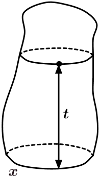
implying the functional relation
| (151) |
It encodes the following geometric situation: each configuration appearing in the path integral has a unique decomposition into a cylinder of proper-time extension (where the proper time is defined as the geodesic distance of the marked point to the boundary), and the disc amplitude itself, as summarized in eq. (151).
Starting from a regularized theory with a cutoff , there are two natural solutions to eq. (151) [45]. In one of them, the regularized disc amplitude diverges with the cutoff and the geodesic distance scales canonically with the lattice spacing according to
| (152) | |||||
| (153) |
In the other, the scaling goes as
| (154) | |||||
| (155) |
where the subscript “reg” denotes the regularized quantities in the discrete lattice formulation. The first scaling (152)-(153), with , is encountered in CDT, while the second scaling (154)-(155) is realized in Euclidean gravity [61, 62].
Allowing for the creation of baby universes during the “evolution” in proper time (by construction, a process forbidden in CDT) leads to a generalization of (131), namely,
where we have introduced a new coupling constant , associated with the creation of baby universes, and also made the additional dependence explicit in the amplitudes. The graphic illustration of eq. (5.1) is shown in Fig. 5.
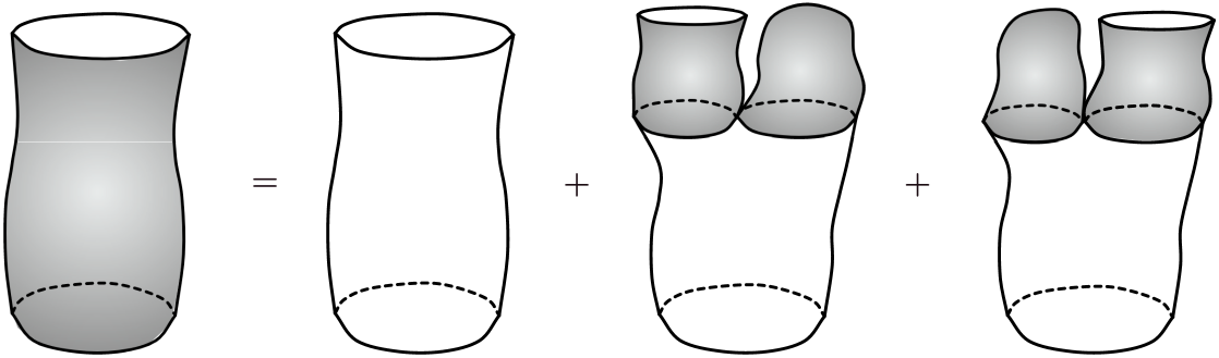
If , i.e. if there is no suppression of baby universes and each geometry with the same area is allowed with the same weight, one obtains precisely the equation known from Euclidean quantum gravity [16]. This happens because according to (152) and (154), we have either , which is inconsistent with (5.1), or we have from (154) that and thus , which is consistent with (154). Thus, in the limit the CDT term disappears and on Fig. 5 we are left with the shaded part and eq. (5.1) reduces to
| (157) |
On the other hand, setting , thereby forbidding the creation of baby universes, leads of course back to (131).
In the case of CDT, where , eq. (5.1) does not contain any reference to the disc amplitude and we can solve for , and subsequently find the disc amplitude, defined e.g. by (148). In Euclidean quantum gravity and the term vanishes in the limit . However, now eq. (157) contains the unknown disc amplitude . The disc amplitude can be found independently [61], but it can also be found by combining (157) and (151). Note that due to (154) eq. (151) reads:
| (158) |
If we integrate (157) with respect to from zero to infinity and with respect to and use (158) on the right-hand side, we obtain
| (159) |
which has the Euclidean gravity solution
(see [45] for details). Thus “quantum geometry” considerations alone entirely determine the disc amplitude and the cylinder amplitude both in CDT and Euclidean two-dimensional quantum gravity.
From the above discussion it is clear that if we start from the CDT model where no baby universe creation is allowed, and then drop this geometric constraint, we end up with Euclidean two-dimensional quantum gravity. This was already discussed in the original article which introduced CDT [45]. However, it is interesting that the CDT model can also be viewed as an “effective” model of Euclidean gravity. It is possible to define in a precise way the concept of “integrating out” baby universes, at the level of the discretized geometries which appear in the path integral defining Euclidean two-dimensional quantum gravity. By doing so one arrives at the CDT model [64].
The CDT and Euclidean models were characterized by being purely geometric. It is possible to find an interpolating model, different from CDT, but with the same scaling, but still allowing for baby universes during the time evolution like the Euclidean model. The price is the introduction of a new coupling constant, the already included in eq. (5.1). By allowing the coupling constant to be a function of the cutoff it is possible to make the “kinetic” CDT term of the same strength as the baby universe term if we assume
| (160) |
where is a coupling constant of mass dimension three, which is kept constant when . With this choice, eq. (5.1) is turned into
| (161) |
The graphical representation of eq. (161) is the one given in Fig. 5. It is clear that while the creation of baby universes can take place, they are severely suppressed by the scaling of , compared to the Euclidean case where they completely dominate over the CDT-like, ordinary propagation.
While the disc amplitude is at this stage unknown, it is possible to obtain an equation for by the same methods as used for the purely Euclidean case just discussed (see [55] for details). The model can also be extended to include higher topologies [56], and it is possible to find a closed expression for the disc amplitude summed over all genera [63].
5.2 Coupling to matter
At a formal level it is easy to couple matter to CDT quantum gravity in two dimensions as well as in higher dimensions. In this subsection we describe the results obtained for two-dimensional CDT, exemplified by the coupling of the Ising model to CDT-gravity.
The presence of the time slicing makes it natural to put the Ising spins at the vertices since they are located at the discrete times defined by the lattice. However, this assignment is not important; one could just as well have placed the spins at the triangle centres. For simplicity we assume that the time is defined to be periodic. This implies that our two-dimensional lattice has the topology of a torus where the number of steps in the time direction is fixed to , while the length of a spatial slice can fluctuate dynamically. The partition function can be written as
| (162) |
where is the CDT-class of triangulations of toroidal topology as described, is the cosmological constant, the number of triangles in the triangulation , and denotes the Ising model on the lattice defined by the triangulation , that is,
| (163) |
In eq. (163) we sum over the spin variables located at vertices , while denotes the link connecting neighbouring vertices and . The parameter is the spin coupling constant divided by the temperature. The Ising spin variable can take values . The generalization for which the spin variable can take the values leads to the -state Potts model. We can write eq. (162) as
| (164) |
where is the CDT-class of triangulations defined as above, but constrained to have triangles.
In general one expects a leading behaviour of the form
| (165) |
which means that we can view as the free energy density at for the ensemble of random lattices when the size goes to infinity. If the spin system defined on this ensemble has a phase transition from a low-temperature magnetized phase to a high-temperature phase with magnetization zero at a certain value , this fact will show up as a discontinuity in the derivative of at at a certain order, depending on the order of the phase transition. It is also possible that the exponent can be discontinuous at .
The same construction works for the DT-class of triangulations. In this case it is possible to solve the discretized models analytically using a mapping to matrix models [65]. The solution reveals that at a certain critical (inverse) temperature there is a third-order phase transition from a magnetized phase (high ) to a phase at low where the magnetization is zero. The critical exponents associated with this transition differ from the flat-space Onsager exponents and agree with the so-called KPZ exponents [66], which can be calculated because two-dimensional Euclidean quantum gravity coupled to conformal field theories with central charge can be solved analytically by conformal bootstrap [66]. For , when the spin system is not critical, the geometric properties of the coupled geometry-spin system are identical to that of two-dimensional Euclidean quantum gravity without matter. However, at the geometric properties of the coupled system change from that of “pure” Euclidean gravity to something else, for example, the entropy exponent changes from to at . This value, first calculated in [65], is in agreement with the continuum calculation [66].
The results for CDT quantum gravity coupled to the Ising model are different from the KPZ results. At this stage it has not been possible to solve the combined model analytically in the same way as in Euclidean two-dimensional gravity coupled to matter. One can resort to strong-coupling expansions and Monte Carlo simulations, with both methods showing that there is a phase transition between a magnetized and an unmagnetized phase [52]. The critical matter exponents found are the (flat-space) Onsager exponents. In addition, the entropy exponent in eq. (165) is equal to 1/2 for all values of , including , with evidence of similar results for the three-state Potts model [53]. In two dimensions, the coupling between geometry and matter therefore appears to be weaker for CDT than for Euclidean gravity. This should not come as a surprise since we have already seen that one can view CDT in two dimensions as an “effective” version of 2d Euclidean quantum gravity, where baby universes have been integrated out. At the same time there exist persuasive arguments explaining the difference between the flat-space Onsager and the KPZ exponents by the presence of baby universes [67]. Following this logic it is then not surprising that two-dimensional CDT gravity coupled to conformal matter gives rise to flat-spacetime exponents. It would be very interesting if the result could be derived from the Euclidean model by integrating out baby universes, in the same way as pure CDT can be obtained from the pure Euclidean model. Until now the fact that one has to integrate over the matter configurations at the boundaries of the baby universes has prevented us from imitating the pure-gravity construction.
6 Changing geometries: Monte Carlo moves
6.1 The need for Monte Carlo simulations
We have used the two-dimensional model as an illustration of how one can obtain a continuum limit of “quantum geometry”, starting from a discretized lattice theory. This is a nontrivial proof of principle, but our main interest is of course the fully fledged four-dimensional theory of quantum gravity. We expect this theory to behave differently, reflecting the presence of true propagating degrees of freedom (suitable nonperturbative analogues of the “gravitons” of the linearized theory) and the fact that it is a nonrenormalizable field theory.
From this point of view, three-dimensional quantum gravity has a place in between two- and four-dimensional quantum gravity. It has a nontrivial Einstein-Hilbert action, and associated with it a formally nonrenormalizable gravitational coupling constant. However, since three-dimensional gravity has no propagating degrees of freedom, it most likely will tell us nothing about the problem of nonrenormalizability. The fact that physical results depend only on a finite number of degrees of freedom (and therefore no field degrees of freedom) suggests that the (quantum) theory could be exactly solvable, like the two-dimensional quantum theory. There have been a number of attempts to solve the three-dimensional CDT theory analytically, so far with only limited success, due to the difficulty of generalizing the exact solution methods to three dimensions [68, 69, 70]. Thus, even in three dimensions, to make progress beyond these results, we must turn to numerical methods [71, 72], a situation also shared by general, non-gravitational lattice models.
Also in four dimensions we have presently no analytic tools for tackling the CDT path integral directly. The results reported below for four-dimensional CDT quantum gravity are based on Monte Carlo simulations, using the action (73). In the remainder of this section we will discuss how to conduct Monte Carlo simulations for causal dynamical triangulations, which are important even in lower dimensions. Neither the two-dimensional model with matter coupling nor the three-dimensional model (with and without matter) have so far been solved analytically.
6.2 Monte Carlo simulation with dynamical lattices
Conventional Monte Carlo simulations in quantum field theory use a fixed lattice of (Euclidean) spacetime, and have fields defined on this fixed lattice. The theory is defined by a partition function
| (166) |
where we sum over all field configurations on the lattice. Let be an observable depending on the fields. Using the path integral we can in principle calculate the expectation value
| (167) |
The purpose of the Monte Carlo simulations is to generate a sequence of statistically independent field configurations , with the probability distribution
| (168) |
Then
| (169) |
serves as an estimator of the expectation value (167) and one has
| (170) |
One starts out with a field configuration or, more generally, with a probability distribution . One then performs certain changes, starting from or, more generally, from a sequence of configurations chosen with probability . These changes are accepted or rejected according to certain criteria which ensure that field configurations after sufficiently many changes will occur with the correct weight (168), dictated by the path integral. In a Monte Carlo simulation a change of the field configuration is usually generated by a stochastic process , a Markov chain. The field will perform a random walk in the space of field configurations with a transition function, or transition probability, . Thus, if after a certain number of steps (changes of the field configuration) we have arrived at a field configuration , is the probability of changing to in the next step. We have
| (171) |
The transition probability should be chosen such that
-
(i)
any field configuration can be reached in a finite number of steps (ergodicity);
-
(ii)
the probability distribution of field configurations converges, as the number of steps goes to infinity, to the Boltzmann distribution (168).
The convergence of the Markov chain is usually ensured by choosing to satisfy the so-called rule of detailed balance
| (172) |
Starting out with an initial configuration or, more generally, an initial probability distribution of configurations , the stochastic process will after steps have generated a new probability distribution . The relation between and is
| (173) |
Using the identity (171), the right-hand side of this equation can be written as
| (174) |
According to relations (173) and (174), the rule (172) of detailed balance ensures that the distribution is a stationary distribution under the stochastic process . We refer to standard textbooks for a proof that converges to . Basically, the detailed-balance condition tells us that is the unique eigenvector of with eigenvalue one, whereas all other eigenvectors have smaller eigenvalues.
A solution to (172) is that either or
| (175) |
Usually one chooses to be nonzero only if some notion of distance between and is small, since else most attempted changes will be rejected. On the other hand, the class of nonvanishing transition amplitudes among the configurations must satisfy the condition of ergodicity, so it cannot be too restricted. The choice of nonvanishing transition amplitudes has a crucial influence on the efficiency of the algorithm. Using (175), one usually decomposes the transition probability into a selection probability and an acceptance ratio . According to eq. (175) we then have
| (176) |
The selection probability is now designed to select the configurations , where is different from zero and assigns a weight of our choice to the transition . The acceptance ratio should then be chosen to ensure detailed balance in the form (176). A general choice, used in many Monte Carlo simulations, is the so-called Metropolis algorithm, defined by
| (177) | |||||
| (178) |
In standard lattice field theory the lattice is fixed and not part of the dynamics. For quantum gravity models based on dynamical triangulations the situation is different. The lattice is represented by an abstract triangulation, which itself represents a curved spacetime geometry. In the path integral we sum over all triangulations, each associated with an action and thus a weight. It is the lattice itself which changes in this type of quantum gravity model. The Monte Carlo simulation must be set up to move us around in the class of abstract CDT triangulations with the correct weight.
In Euclidean quantum gravity models, where one performs the summation over all abstract triangulations of a fixed topology, the so-called Pachner moves [73] are a minimal set of local topology-preserving changes of the triangulations which are ergodic. This means that by repeated use of these “moves” it is possible to get from one triangulation of a certain topology to any other of the same topology. In the computer we work with labeled triangulations. Thus the partition function will be represented in the numerical simulations as a sum over labeled triangulations, as described in the discussion surrounding eq. (75) in Sec. 3. Speaking in general terms, the computer then keeps a list of the vertices of the triangulation, for each vertex a list of all the neighbouring vertices and a list of how this set of points is organized into simplices and subsimplices. There are many different ways to organize and store this information. It is not our intention to go into a detailed discussion of this, but in the next subsection we will give an example of how this can be done in the very simple case of two-dimensional CDT, and how the tables are updated when a move is performed.
The Pachner moves used in Euclidean dynamical triangulations are not directly applicable in CDT since they generally do not respect the sliced structure of the Lorentzian discrete geometries. Our strategy for constructing suitable sets of moves is to first select moves that are ergodic within the spatial slices (this is clearly a necessary condition for ergodicity in the complete set of four-dimensional triangulations of fixed topology), and then supplement them by moves that act within the sandwiches . In manipulating triangulations, especially in four dimensions, it is useful to know the numbers of simplicial building blocks of type A contained in a given building block of type B of equal or larger dimension (Table 1).
If the moves are used as part of a Monte Carlo updating algorithm, they will be rejected whenever the resulting triangulation would violate the simplicial manifold constraints. The latter are restrictions on the possible gluings (the pairwise identifications of subsimplices of dimension ) to make sure that the boundary of the neighbourhood of each vertex has the topology of a -sphere [40]. In dimension three, “forbidden” configurations are conveniently characterized in terms of the intersection pattern of the triangulation at some half-integer time. The latter is given by a two-dimensional tessellation in terms of squares and triangles or, alternatively, its dual three- and four-valent graph (see Appendix 2 in [71] for details). Also in four dimensions, one may characterize sandwich geometries by the three-dimensional geometry obtained when cutting the four-dimensional geometry at a half-integer time between two adjacent spatial triangulations height. The corresponding three-dimensional geometry consists of two types of three-dimensional building blocks, tetrahedra and prisms (see also [74]).
| contains | ||||||||||
|---|---|---|---|---|---|---|---|---|---|---|
| 1 | 2 | 2 | 3 | 3 | 4 | 4 | 4 | 5 | 5 | |
| 1 | 0 | 2 | 0 | 3 | 4 | 0 | 4 | 6 | ||
| 1 | 1 | 3 | 3 | 2 | 6 | 6 | 4 | |||
| 1 | 0 | 3 | 4 | 0 | 6 | 9 | ||||
| 1 | 1 | 0 | 4 | 4 | 1 | |||||
| 1 | 0 | 0 | 4 | 2 | ||||||
| 1 | 0 | 0 | 3 | |||||||
| 1 | 1 | 0 | ||||||||
| 1 | 0 | |||||||||
| 1 |
To summarize: the moves define the possible changes we can make to go from one triangulation to another. Thus they serve precisely as part of the section function mentioned above. In this way the moves allow us to define the selection function mentioned above. As a next step, we choose the acceptance ratio such that detailed balance is satisfied for a particular move and its “inverse”. In the next subsections we will describe the CDT moves in two, three and four dimensions explicitly. In addition, we will discuss how the functions and are determined in two dimensions.
6.3 Moves in two dimensions
The two-dimensional case is simple. Two moves which are ergodic and respect the CDT structure of spacetime are shown in Fig. 6. We denote the two moves by (2,2) and (2,4). The (2,2)-move takes two adjacent triangles positioned as shown in Fig. 6, that is, a (1,2)- and a (2,1)-triangle sharing a timelike link, and flips the diagonal, thus not changing the boundary of the subcomplex consisting of the two triangles. Similarly, the (2,4)-move takes two adjacent triangles sharing a spacelike link and replaces the two triangles by four triangles, as shown in Fig. 6. Again, the boundary of this new subcomplex is identical to the boundary of the original subcomplex consisting of the two adjacent triangles. The inverse move, a (4,2)-move, takes a vertex of order four and deletes it, together with the two timelike links and one of the spacelike links sharing the vertex. As a result, two triangles are deleted and one is left with a subcomplex of two adjacent triangles sharing a spacelike link. If we use the labeling of vertices shown in Fig. 6, the changes are encoded by writing for the (2,2)-move
| (179) |
and similarly for the (2,4)-move
| (180) |
The labeling denotes a triangle consisting of vertices with labels , and , regardless of their orientation. Similarly, denotes a link. Thus 123+234 stands for a subcomplex whose triangles share link 23, while the boundary is made of the links which are not shared, i.e. 12, 13, 24 and 34. This “algebraic” representation is very convenient and can be generalized in a straightforward manner to higher dimensions. It is the one used in the computer. For example, in four dimensions two four-simplices 12345 and 23456 will share the tetrahedron 2345.

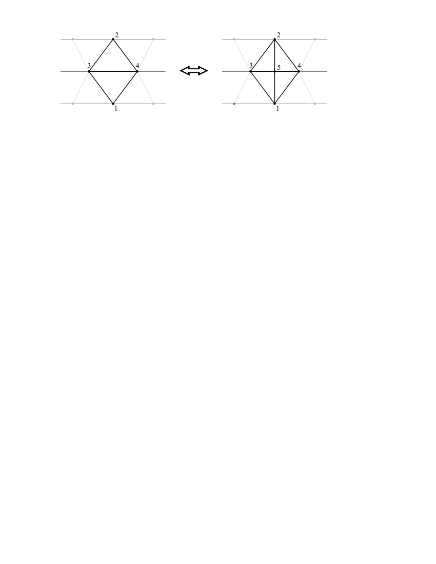
Let us use the two-dimensional case to discuss the detailed-balance aspect of the Monte Carlo updating, since it is slightly more complicated than in ordinary lattice Monte Carlo simulations. Given is the space of configurations, in this case, the abstract two-dimensional triangulations with the topology of a cylinder, satisfying the CDT requirements. To simplify the discussion of boundaries let us compactify the time direction, thereby creating a torus. In the computer we work with labeled triangulations, with the action given by (90). For a given triangulation , since the number of triangles is two times the number of vertices , we have . Since we work with labeled triangulations in the computer, according to (75) the probability assigned to a given triangulation is given by
| (181) |
Let us consider the (2,4)-move and its inverse. In order to have an ergodic set of moves we will also need to invoke the (2,2)-move, which we will simply do by alternating with a suitable frequency between (2,4)- and (2,2)-moves. We require detailed balance for the (2,4)-move and its inverse. According to (176) we write
| (182) |
Given a labeled triangulation and performing move (2,4), we create a new labeled triangulation with vertices. If the old vertices are labeled 1 to , we assign the label to the new vertex. (New links and triangles are defined by pairs and triples of vertex labels, the triples also defining the correct orientation.) Starting from a labeled triangulation we can construct labeled triangulations by choosing different vertices and performing the (2,4)-move. We define the selection probability to be the same for all triangulations that can be reached in this way and zero for all other labeled triangulations. For the labeled triangulations which can be reached in this way we have
| (183) |
We implement this in the computer program by choosing randomly with uniform probability a vertex in .
Given a labeled triangulation we perform the (4,2)-move as follows. Select the vertex labeled , and assume for the moment it is of order four. Delete it from the list, in this way creating a labeled triangulation . If the vertex labeled is not of order four do not perform the move.111111One is free to avoid this situation by keeping a list of vertices of order four and choosing at random one of these vertices, rather than the one with label . This can be viewed as redefining the labeling, interchanging the label of the chosen vertex with the vertex labeled , and reassigning the labeling of links and triangles correspondingly. Of course, we do not really have to make the reassignment in the computer since all labelings are equivalent. Thus, for the triangulations where the move can be performed we can only reach one triangulation and the selection probability defined by this procedure is one. Finally, choose the acceptance ratios in accordance with the Metropolis algorithm, (177)-(178) as
| (184) | |||||
| (185) |
The line of argument given here for the (2,4)-move applies to all moves discussed below, namely, one first chooses a suitable selection probability and then adjusts the acceptance ratio accordingly, such that the detailed-balance equation is satisfied.
6.4 Moves in three dimensions
For the three-dimensional CDT triangulations there are five basic moves (counting inverse moves as separate) [71, 76]. They map one three-dimensional CDT triangulation into another, while preserving the constant-time slice structure, as well as the total proper time . We label the moves by how they affect the number of simplices of top-dimension, i.e. . A -move is one that operates on a local subcomplex of tetrahedra and replaces it by a different one with tetrahedra. In all cases the two-dimensional boundaries of the two subcomplexes are identical121212The notation of a -move can be generalized to any dimension . We have already used it in the case for the (2,2)-move and the (2,4)-move. We have two subcomplexes consisting of and -simplices, but with identical -dimensional boundaries.. The tetrahedra themselves are characterized by 4-tuples of vertex labels. Throughout, we will not distinguish moves that are mirror images of each other under time reflection. In detail, the moves are
-
(2,6):
this move operates on a pair of a (1,3)- and a (3,1)-tetrahedron (with vertex labels 1345 and 2345) sharing a spatial triangle (with vertex labels 345). A vertex (with label 6) is then inserted at the centre of the triangle and connected by new edges to the vertices 1, 2, 3, 4 and 5. The final configuration consists of six tetrahedra, three below and three above the spatial slice containing the triangles (Fig. 7). This operation may be encoded by writing
(186) where the shared triangles on the right-hand side of the arrow have labels 346, 356 and 456. The inverse move (6,2) corresponds to a reversal of the arrow in (186). Obviously, it can only be performed if the triangulation contains a suitable subcomplex of six tetrahedra.
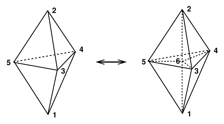
Figure 7: The (2,6)-move in three dimensions. -
(4,4):
This move can be performed on a subcomplex of two (1,3)- and two (3,1)-tetrahedra forming a “diamond” (see Fig. 8), with one neighbouring pair each above and below a spatial slice. The move is then
(187) From the point of view of the spatial “square” (double triangle) 2345, the move (187) corresponds to a flip of its diagonal. It is accompanied by a corresponding reassignment of the tetrahedra constituting the diamond.

Figure 8: The (4,4)-move in three dimensions. The (2,6)- and (6,2)-moves, together with the (4,4)-move (which is its own inverse) induce moves within the spatial slices that are known to be ergodic for two-dimensional triangulations.
-
(2,3):
The last move, together with its inverse, affects the sandwich geometry without changing the spatial slices at integer-. It is performed on a pair of a (3,1)- and a (2,2)-tetrahedron which share a triangle 345 in common (see Fig. 9), and consists in substituting this triangle by the one-dimensional edge 12 dual to it,
(188) The resulting configuration consists of one (3,1)- and two (2,2)-tetrahedra, sharing the link 12. Again, there is an obvious inverse.
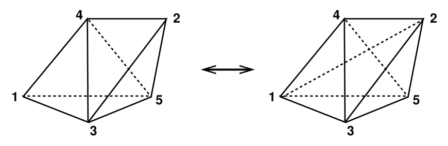
Figure 9: The (2,3)-move in three dimensions.
6.5 Moves in four dimensions
If we distinguish between the space- and timelike character of all of the four-dimensional moves, there is a total of ten moves (including inverses). We will again characterize simplices in terms of their vertex labels. The first two types of moves, (2,8) and (4,6), reproduce a set of ergodic moves in three dimensions when restricted to spatial slices. We will describe each of the moves in turn [76].
-
(2,8):
The initial configuration for this move is a pair of a (1,4)- and a (4,1)-simplex, sharing a purely spacelike tetrahedron 3456 (Fig. 10).

Figure 10: The (2,8)-move in four dimensions. The move consists in inserting an additional vertex 7 at the center of this tetrahedron and subdividing the entire subcomplex so as to obtain eight four-simplices,
with an obvious inverse.
-
(4,6):
In this configuration, we start from a pair (2345,3456) of spatial tetrahedra sharing a common triangle 345, which are connected to a vertex 1 at time and another vertex 7 at time , forming together a subcomplex of size four (Fig. 11). The move consists in swapping the triangle 345 with its (spatially) dual edge 26, during which the two spatial tetrahedra are substituted by three, and the geometry above and below the spatial slice at time changes accordingly. In our by now familiar notation, this amounts to
with the arrow reversed for the corresponding inverse move.
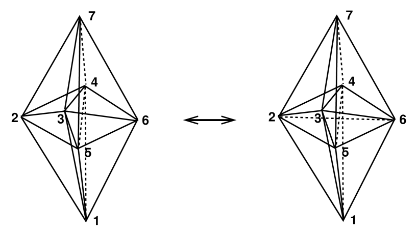
Figure 11: The (4,6)-move in four dimensions. -
(2,4):
This type of move comes in two varieties. Its general structure is as follows: the initial configuration is a pair of four-simplices with a common tetrahedron. During the move, this tetrahedron is “deleted” and substituted by its dual (in a four-dimensional sense) edge. The end result is a subcomplex consisting of four 4-simplices. From a Lorentzian point of view, there are two situations where the application of this move does not interfere with the slice-structure or the manifold constraints. In the first one, a (4,1)- and a (3,2)-tetrahedron from the same sandwich share a (3,1)-tetrahedron 3456 (Fig. 12). The dual edge 12 is timelike and shared in the final configuration by one (4,1)- and three (3,2)-simplices. The second possibility is that of two (3,2)-simplices sharing a (2,2)-tetrahedron. One of the (3,2)-simplices is “upside-down”, such that the entire subcomplex has spatial triangles in both the slices at and at (134 and 256, see Fig. 13). After the move, the total number of (3,2)-simplices has again increased by two. Both types of moves are described by the relation
(191) and their inverses by the converse relation.
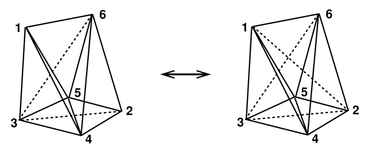
Figure 12: The (2,4)-move in four dimensions, first version. 
Figure 13: The (2,4)-move in four dimensions, second version. -
(3,3):
The initial subcomplex in this type of move is made up of three 4-simplices which share a triangle in common. In the course of the move, this triangle is “deleted” and substituted by its dual (in a four-dimensional sense), which is again a triangle. It is straightforward to verify that this move can only occur in Lorentzian gravity if both of the triangles involved are timelike. Again, there are two allowed variations of the move. In the first one, both the initial and final subcomplex consist of one (4,1)- and two (3,2)-simplices, and the spacelike edge of each of the triangles 123 and 456 lies in the same slice (Fig. 14). The four-simplices are rearranged according to
(192) 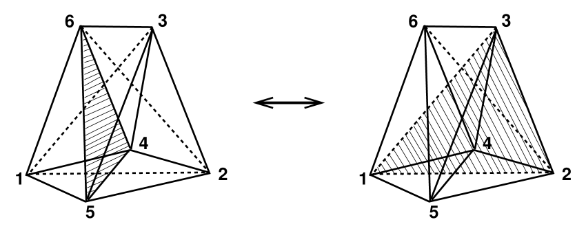
Figure 14: The (3,3)-move in four dimensions, first version. 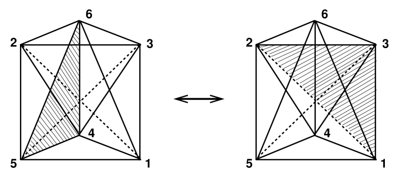
Figure 15: The (3,3)-move in four dimensions, second version. The other initial configuration for which (192) can be performed involves only (3,2)-simplices of both orientations, as illustrated in Fig. 15. The “swapped” triangle 123 now has its spacelike edge in the opposite spatial slice from that of the original triangle 456. As in the (4,4)-move in three dimensions, this type of move is its own inverse.
7 The entropic nature of CDT and the phase diagram
We are now ready to set up Monte Carlo simulations of the four-dimensional CDT quantum gravity model. We store the simplicial geometry as a set of lists, which consist of sequences of labels for simplices of dimension , , together with their position and orientation with respect to the time direction. Additional list data include information about nearest neighbours, i.e. how the triangulation “hangs together”, and other discrete data (for example, how many four-simplices meet at a given edge) which help improve the acceptance rate of Monte Carlo moves.
The simulation is set up to generate a random walk in the ensemble of causal geometries of a fixed time extension . We are of course interested in conducting the simulations with triangulations that are as large as possible. However, since the moves used to change the triangulation are local, the time it takes to change a given triangulation into a new “independent” triangulation will increase with the size of the triangulation. Thus one has to find a compromise between (computer) time and size. Until now we have used triangulations which consists of up to 362.000 four-simplices. To get an idea of the corresponding linear size, suppose we organized the four-simplices such that they approximately formed a regular four-dimensional lattice. The size of this lattice turns out to be up to . While we are working with our dynamically generated universe in the computer, hoping to find measurable observables, it is worth keeping in mind that we are trying to squeeze the universe into a lattice! Not unlike in lattice QCD, this obviously limits the kind of questions we can ask. Clearly, if we added matter, it would be difficult to study the formation of galaxies, even if we could manage to find a way to address this question after rotating to Euclidean signature.
7.1 The entropic nature of CDT and the continuum limit
The action we are using is (73) is a compact rewriting of the Einstein-Hilbert action (2.9.3). There are three coupling constants, , and , where is related to the cosmological coupling constant as described in Sec. 2.9.3 and dictates the average number of . The cosmological-constant term contributes at the same leading order as the entropy (the number of triangulations with a given number of four-simplices), which also grows exponentially with [41]. We encountered a similar phenomenon in the two-dimensional model which could be solved analytically (see (125)).131313Contrary to the situation in two dimensions there is no analytic proof of the exponential bound in three- or four-dimensional DT. At some stage, there were claims (based on Monte Carlo simulations) that the number grows much faster [75]. However, it is now generally believed that the growth is only exponential as a function of . As discussed in connection with (125), the exponential growth defines a critical point, to which one has to fine-tune the bare cosmological constant. If the bare cosmological constant is smaller than the critical value, the partition function is simply ill defined. If it is larger than the critical value the expectation value will remain finite even as . We test arbitrarily large values of when fine-tuning the bare cosmological constant to its critical value, precisely as in the two-dimensional case. In addition, the renormalized, physical cosmological constant is defined by this approach to the critical value, again like in two dimensions. However, the subleading correction to the exponential growth of the number of triangulations, i.e. the function in (125) in the two-dimensional case, can be different.
Let us make the discussion more explicit to illustrate the analogy with the two-dimensional case and to emphasize the role of “entropy”, i.e. the number of configurations. We can write the partition function as
| (193) |
Introducing
| (194) |
this can be rewritten as
| (195) |
where denotes the number of CDT configurations with four-simplices, of which are of type or , and with vertices, including symmetry factors. We conclude that the calculation of the partition function is in principle a combinatorial problem, just as in two dimensions where we could solve the problem explicitly. Our rationale for calling the model entropic is that the partition function is entirely determined by the number of geometries in the simplest possible way, in the sense of being the generating function for these numbers. The logarithm of the number of geometric “microscopic” configurations for given numbers is proportional to their entropy in the sense of statistical models.141414For a statistical system, like a spin system, the entropy is defined as (proportional to) the logarithm of the number of states which appear in the definition of the partition function as a state sum. When talking about “entropy”, it is by analogy with such statistical systems. However, while a “state” in the classical partition function for spins can be considered as physical, a “history” contributing to the path integral in quantum field theory (or in quantum mechanics) is not physical. After rotation to Euclidean time, the path integral can be viewed as partition function of a (virtual) statistical system. It is only in this sense that we talk about the entropy of geometries. Unlike in two dimensions, it has until now not been possible to solve this counting problem analytically. As mentioned above, one cannot even prove the exponential bound. This means that we will in the first place probe the properties of (193) with numerical methods.
Let us now turn to the renormalization of the cosmological constant by fine-tuning . We write the partition function as
| (196) |
where is the partition function for a fixed number of four-simplices, namely,
| (197) |
As already mentioned, there is numerical evidence that is exponentially bounded as a function of [41],
| (198) |
where grows slower than exponentially. We call the critical value of . It is a function of and and plays the same role as in the two-dimensional model discussed above: the partition function is only defined for and the “infinite-volume” limit, where can only be achieved for . We are interested in sending the lattice spacings to zero while keeping the physical four-volume, which is roughly , fixed. Thus we want to consider the limit , and fine-tune to for fixed . This fine-tuning is similar to the fine-tuning in the two-dimensional model. Like there, we expect the physical cosmological constant to be defined by the approach to the critical point according to
| (199) |
which is the counterpart to (127). It ensures that the term
| (200) |
gives rise to the standard cosmological term in the Einstein-Hilbert action. Thus the fine-tuning of brings us to the limit of infinite four-volume. It does not necessarily imply a continuum limit too. The situation here may be different from that of the two-dimensional model, where approaching automatically implied a continuum limit. Two-dimensional quantum gravity is of course a very simple model with no propagating degrees of freedom, which we do expect to be present in four-dimensional quantum gravity. Thus the situation is more like in ordinary Euclidean lattice field theory/critical phenomena, where “infinite volume” does not necessarily mean “continuum limit”.
A good example of what one might expect is the Ising model on a finite lattice. To obtain a phase transition for this model one has to take the lattice volume to infinity, since there are no genuine phase transitions for finite systems. However, just taking the lattice volume to infinity is not sufficient to ensure critical behaviour of the Ising model. We also have to tune the coupling constant to its critical value, at which point the spin-spin correlation length diverges. Similarly, in CDT, having adjusted we have to search the coupling constant space of and in order to find regions where we do not only have an infinite four-volume limit but also an interesting limit from the point of view of continuum physics.
How can one imagine obtaining an interesting continuum behaviour as a function of ? For purposes of illustration we ignore and assume that the subleading correction has the form
| (201) |
(We will later on check numerically that such a term is indeed present.) The partition function now becomes
| (202) |
For dimensional reasons we expect the classical Einstein term in the action to scale like
| (203) |
motivating the search for a value with , with the approach to this point governed by
| (204) |
With such a choice we can identify a continuum limit where , calculated from (202) (by a trivial saddle point calculation), goes to infinity while ,
| (205) |
Thus we find
| (206) |
as one would naïvely expect from Einstein’s equations, with the partition function being dominated by a typical instanton contribution, for a suitable constant .
7.2 Set-up of computer simulations
The actual set-up for the computer simulations is slightly different from the theoretical framework discussed above, in that we choose to work with a fixed number of four-simplices , rather than fine-tuning to its critical value. We can perform computer simulations for various (and fixed ) and in this way check scaling with respect to . This is an alternative to fine-tuning , and much more convenient from a computational point of view. For large we can then check whether there are any finite-size effects or whether effectively we have already reached the infinite-volume limit. At a formal level we can perform a Laplace transformation of the partition function,
| (207) |
where
| (208) |
is the partition function for a constant four-volume and the gravitational action without the cosmological term. The expectation values we are calculating are thus
| (209) |
It is in principle possible to reconstruct the expectation values of observables for a fixed value of the cosmological constant by measuring the for all and constructing (which cannot be measured as an observable in a Monte Carlo simulation). This reconstruction is somewhat cumbersome but feasible, since the action only depends on the “global” variables , and . However, we will restrict ourselves to the measurement of observables for fixed .
The local moves do not in general preserve the numbers and of four-simplices, or their sum. We deal with this in a standard way which was developed for dynamically triangulated models in dimensions three and four [10, 13] to ensure that the system volume is peaked at a prescribed value, with a well-defined range of fluctuations. Adapting it to the current situation of causal triangulations with nonvanishing asymmetry , we implement an approximate four-volume constraint by adding a term
| (210) |
to the Euclidean action (73), with typical values of lying in the range of 0.01 to 0.02, except during thermalization where we set . The reason for fixing instead of in eq. (210) is mere technical convenience. We have checked in the phase space region relevant to four-dimensional quantum gravity (phase C, see below) that for fixed according to (210), the number of four-simplices of type (3,2) is likewise peaked sharply, see Fig. 16.
| “four-volume” | 10 | 20 | 40 | 80 | 160 |
|---|---|---|---|---|---|
| actual four-volume | 22.25 | 45.5 | 91 | 181 | 362 |
The “four-volumes” and the corresponding “true” discrete four-volumes used in the simulations are listed in Table 2 for well inside phase C, at the choice of coupling constants where most of our simulations are performed.
\psfrag{V}{\bf{\Large$N_{4}^{(3,2)}$}}\psfrag{P(V)}{\Large\bf$P(N_{4}^{(3,2)})$}\includegraphics{volumes.ps}
In order to stabilize the total volume after thermalization, has to be fine-tuned to its pseudo-critical value (which depends weakly on the volume) with accuracy smaller than , in practice to about . The measurements reported in this paper were taken at 10, 20, 40, 80 and 160k, and the runs were performed on individual PCs or a PC farm for the smaller systems and a cluster of work stations for the larger systems.
Before measurements can be performed, one needs a well thermalized configuration of a given volume. In order to double-check the quality of the thermalization, we used two different methods to produce starting configurations for the measurement runs. In the first method, we evolved from an initial minimal four-dimensional triangulation of prescribed topology and given time extension , obtained by repeated gluing of a particular triangulated spacetime slice (a “slab”) of (one lattice step in the time direction) and topology , which consists of 30 four-simplices. The spatial in- and out-geometries of the slice are minimal spheres , made of five tetrahedra. The two types of spatial boundary conditions used are (i) periodic identification of the geometries at initial and final integer times, and (ii) free boundary conditions, where all vertices contained in the initial slice at time are connected by timelike edges to a single vertex at time , and similarly for the vertices contained in the final spatial slice. From this initial configuration, the geometry evolves to its target volume as specified in . During the evolution the volume-volume correlator (to be defined below) was monitored and used to gauge the auto-correlation of configurations. The number of sweeps to reach the thermalized configuration changes linearly with and ranged from to sweeps for the largest volumes, the latter of which took several weeks on a work station.
In the second method, we started instead from a thermalized configuration of smaller volume, which we let evolve towards the target volume. In this case the final volume-volume distribution is reached from a narrower distribution, namely, that of the smaller volume. During thermalization, this width grows very slowly. The timing of the entire process is similar to that of the first method.
7.3 Phase structure of the model
As described above, the bare cosmological constant is tuned to its (pseudo-)critical value in the simulations, tantamount to approaching the infinite-volume limit. Depending on the values of the two remaining parameters and in the discretized action (73), we have identified three different phases, A, B and C, mutually separated by phase transition lines [77, 78]. Fig. 17 shows the phase diagram, based on computer simulations with [81]. Because there are residual finite-size effects for universes of this size, one can still expect minor changes in the location of the transition lines as . The dotted lines in Fig. 17 represent mere extrapolations, and lie in a region of phase space which is difficult to access due to inefficiencies of our computer algorithms. Thus the phase diagram is only tentative where the lines are dotted, and in particular the triple point is our invention. However, once we are in the “bulk” of phase A, B and C there are no problems with the simulations. Thus the phase diagram in Fig. 17 is essentially correct in the sense that we have only observed these three phases. Also, moving away from the putative triple point there is eventually no problem in identifying a transition between phases A and B. We have not done so except for the single point shown on Fig. 17 because this phase transition presently does not have our main interest (since we do not know of an interesting continuum interpretation). In summary, the most likely scenario, even without having identified part of the transition lines in detail, is the one presented in Fig. 17.
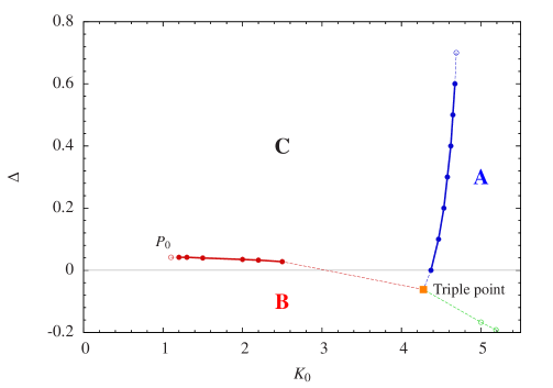
We describe each of the three phases in turn:
-
(A)
This phase prevails for sufficiently large (recall is proportional to the inverse of the bare Newton’s constant). When plotting the volume of the spatial slices of constant as a function of , we observe an irregular sequence of maxima and minima, where the minimal size is of the order of the cutoff, and the sizes of the maxima vary, see Fig. 18. The time intervals during which the spacetime has a macroscopic spatial extension are small and of the order of , being the subscript in .
-
(B)
This phase occurs for sufficiently small and for small asymmetry . In it, spacetime undergoes a “spontaneous dimensional reduction” in the sense that all four-simplices are concentrated in a slice of minimal time extension between and and and , such that the three-volumes at times is only large at time and remain close to their kinematic minimum everywhere else (Fig. 19).

However, there is yet another phase where the dynamics is not reduced to just the spatial directions but is genuinely four-dimensional.
-
(C)
This phase occurs for sufficiently small and nonvanishing asymmetry . In this phase, where and ( was defined above, eq. (2.9.3)), there seems to be a sufficiently strong coupling between successive spatial slices to induce a change in the spatial structure itself. We will discuss this new geometrical structure in detail below in Sec. 8. Stated shortly, we observe a genuine four-dimensional universe, the blob shown in Fig. 20. This blob is four-dimensional in the sense that as a function of the four-volume , the time extent scales as and the spatial volume as (see Fig. 20), and the blob itself is independent of the total time extent chosen, as long as is larger than the time extent of the blob.
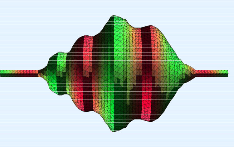
We have performed measurements to determine the order of the transitions in the CDT phase diagram. Based on our numerical investigation so far, the A-C transition appears to be a first-order transition [81], while the B-C transition is second order [82]. Below we report on some details of these measurements.
7.3.1 The A-C transition
The two graphs at the bottom of Fig. 21 illustrate the behaviour of at the A-C phase transition line. Since we can approach this line by changing the coupling constant while keeping fixed, the quantity conjugate to ( is fixed), namely, the ratio , is a natural candidate for an order parameter. The graph at the centre of Fig. 21 shows as a function of Monte Carlo time. One sees clearly that it jumps between two values, corresponding to the distinct nature of geometry in phases A and C. We have checked that the geometry indeed “jumps” in the sense that no smoothly interpolating typical configurations have been found. Lastly, we have also established that the jump becomes more and more pronounced as the four-volume of the universe increases, further underlining the archetypical first-order behaviour at this transition line.
The top graph in Fig. 21 shows the location of the universe along the vertical “proper-time axis” (, and to be periodically identified) as a function of Monte Carlo time, plotted along the horizontal axis. The value of the spatial three-volume in the slice labeled by is colour-coded; the darker, the bigger the volume at time . We can distinguish two types of behaviour as a function of Monte Carlo time, (i) presence of an extended universe centred at and fluctuating weakly around some location on the proper-time axis; (ii) absence of such a universe with a well-defined “centre-of-volume”. The former is associated with the presence of a distinct dark band in the figure, which disappears abruptly as a function of Monte Carlo time, only to reappear at some different location later on in the simulation. Comparing with the middle graph, it is clear that these abrupt changes in geometry correlate perfectly with the changes of the order parameter . When is small, we witness the extended universe of phase C, whose “equator” coincides with the dark blue/red line of the colour plot. Conversely, at the larger values of characteristic of phase A this structure disappears, to be replaced by an array of universes too small to be individually identifiable on the plot. When jumping back to phase C the centre-of-volume of the single, extended universe reappears at a different location in time. Finally, the bottom graph in Fig. 21 illustrates the double-peak structure of the distribution of the values taken by the order parameter .
7.4 The B-C transition
Our measurements to determine the character of the B-C transition are depicted in an analogous manner in Fig. 22. Since we are varying to reach this transition from inside phase C, we have chosen the variable conjugate to in the action (73) (up to a constant normalization ), , as our order parameter. Looking at the graph at the centre, we see that this parameter exhibits the jumping behaviour as a function of Monte Carlo time that is characteristic of a first-order transition. Small values of the parameter indicate the system is in phase C, while large values correspond to phase B. The time extent of the universe diminishes as one approaches the phase transition line from phase C, and is close to zero when we are at the transition line. It is zero when we cross the line. Some indication of this behaviour is given by the colour-coded three-volume profile as a function of the Monte Carlo time in the top graph of Fig. 22. In phase B, only one lattice time has a number of tetrahedra much larger than zero. The “universe” is concentrated on a single time slice, while well inside phase C it has a nontrivial time extension. The bottom graph in Fig. 22 again shows the double-peak structure of the order parameter.
Looking at Fig. 22 and comparing it with the previous Fig. 21, the evidence for a first-order transition at the B-C phase boundary seems even more clear-cut than in the case of the A-C transition.

However, a double peak for a given does not tell us whether the transition is first or second order. One has to establish how the double peak behaves as a function of . If the size of the peaks increases and the separation of the peaks does not diminish when increases it is a strong signal that the transition is first order. This appears to be the situation for the A-C transition. For the B-C transition the opposite happens: the peaks approach each other, approximately as , and the height of the peaks relative to the minimum between the peaks also diminishes, again approximately as . This is shown in Fig. 23. Thus the peak structure does not have the characteristics of a first-order transition.
In order to establish that we are really dealing with a higher-order transition we have looked at various critical exponents. They all point to a higher-order transition. We will limit the discussion here to the so-called shift exponent, (for a detailed discussion we refer to [82]), defined as follows. For fixed , we vary the coupling constant to reach a critical point on the B-C phase transition line. For a system of finite volume, the precise definition of the critical is ambiguous, since there is strictly speaking only a phase transition for . We choose to define using the location of the maximum of the susceptibility . One expects a -dependence of the form
| (211) |
with a first-order transition characterized by . Thus observing a different from 1 is a signal of a higher order transition.
Figure 24 displays the data and the best fit for . We have not included error bars because they turned out to be smaller than the data point dots. The best fit through all data points yields , which is far from the value characterizing a first-order transition. We can perform similar measurements for the other values of along the B-C transition line which are shown in Fig. 17 and establish that for these points the transition seems to be of second (or higher) order.
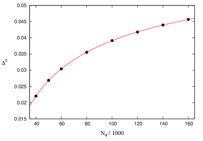
It would be interesting to perform the same measurements moving along the B-C transition line towards the conjectured triple point. However we need more a more efficient algorithm151515As described above, we are basically using the simplest Metropolis algorithm for updating geometry, using the local moves. This local algorithm might be very inefficient when it comes to changing certain types of geometries. In four-dimensional Euclidean DT gravity, one type of geometry which could be created was a so-called baby universe, only connected to the rest of the universe with a thin “neck”. These baby universes were both a blessing and a curse. By counting them one could measure the so-called susceptibility exponent of the partition function [79], but the local moves had a hard time getting rid of them, once they were created. This issue could be resolved by inventing an algorithm that cut away the baby universes in one place and glued them back onto the triangulation in another [80]. This “baby-universe surgery” decreased the auto-correlation time in the simulations by several orders of magnitude. We have been searching for a similar algorithm in the CDT case, but so far without success.. It is possible that a multicanonical algorithm can deal better with the double-peak structure which seems to get more pronounced when we move towards the conjectured triple point.
We have not studied the A-B transition in any detail since it seems not interesting from a gravitational point of view, where we want to start out in a phase with an extended, quasi-classical four-dimensional universe, i.e. in phase C.
7.5 Relation to Hořava-Lifshitz gravity
We can now give the following qualitative characterization of the three phases in terms of what we will provisionally call “average geometry”. As we will show below, the universe of phase C exhibits a classical four-dimensional background geometry on large scales. We may rephrase this by saying that . One may even argue that , in view of the fact that according to the minisuperspace analysis of [83, 84, 85, 86] – to be presented below – the universe can be identified with a round , the maximally symmetric de Sitter space of constant scalar curvature. By contrast, in phase B the universe presumably has no extension or trace of classicality, corresponding to “”. Lastly, in phase A, the geometry of the universe appears to be “oscillating” in the time direction. The three phases are separated by three phase transition lines which we have conjectured to meet in a triple point as illustrated in Fig. 17.
We have chosen this particular qualitative description to match precisely that of a Lifshitz phase diagram [87]. In an effective Lifshitz theory, the Landau free energy density as function of an order parameter takes the form161616see, for example, [88] for an introduction to the content and scope of “Landau theory”
where for a -dimensional system , . Distinguishing between “”- and “”-directions allows one to take anisotropic behaviour into account. For a usual system, and a phase transition can occur when passes through zero (say, as a function of temperature). For we have , while for we have (always assuming ). However, one also has a transition when anisotropy is present () and passes through zero. For negative one can then have an oscillating behaviour of in the “”-directions. Depending on the sign of , the transition to this so-called modulated or helical phase can occur either from the phase where , or from the phase where . We conclude that the phases C, B, and A of CDT quantum gravity depicted in Fig. 17 can be put into a one-to-one correspondence with the ferromagnetic, paramagnetic and helical phases of the Lifshitz phase diagram171717For definiteness, we are using here a “magnetic” language for the Lifshitz diagram. However, the Lifshitz diagram can also describe a variety of other systems, for instance, liquid crystals.. The triple point where the three phases meet is the so-called Lifshitz point.
The critical dimension beyond which the mean-field Lifshitz theory alluded to above is believed to be valid is . In lower dimensions, the fluctuations play an important role and so does the number of components of the field . This does not necessarily affect the general structure of the phase diagram, but can alter the order of the transitions. Without entering into the details of the rather complex general situation, let us just mention that for fluctuations will often turn the transition along the A-C phase boundary into a first-order transition. Likewise, most often the transition between phases B and C is of second order.
As mentioned in the Introduction P. Hořava has suggested recently a new class of quantum gravity theories [26]. The basic idea is that in a theory of quantum gravity one should insist on manifest unitarity as well as renormalizability. These two requirements clash when we use the Einstein-Hilbert action. It contains only second-order time derivatives and in this respect has a chance to be unitary, but it is not renormalizable as we have discussed in detail. In order to obtain a renormalizable theory one can add higher-curvature terms like to the action. Expanding the action around flat spacetime, higher-derivative terms will appear in the quadratic part, making the propagators better behaved at large momenta. As also mentioned in Sec. 1 one can prove that a number of such theories is renormalizable [21]. However, it is believed that in general they will not be unitary, the unitarity being spoiled by the higher-order time derivatives which appear in the propagators. Covariance implies that higher-order derivatives result in higher-order time derivatives, which usually lead to acausal propagation. This conundrum can be avoided if we give up covariance and allow space and time to behave differently. Having higher-derivative spatial terms but only second-order time derivatives in the equations of motion makes it possible to construct a unitary and renormalizable theory. The price one pays is that local Lorentz invariance is broken. Since we know that Lorentz invariance is valid to a good approximation at large distances, the terms which break Lorentz invariance have to be suitably small, such that they only play an important role at high (spatial) momenta. Hořava used the Lifshitz free energy (7.5) as an example where higher-derivative terms play an important role and where there is asymmetry between the various (spatial) directions181818In the Lifshitz free energy density (7.5) all directions are of course spatial directions, but the derivative terms break the symmetry. In the Hořava-Lifshitz model, the asymmetry is between space directions and time. After a formal rotation to Euclidean signature the Hořava Lagrangian would be a Lifshitz-like free energy density..
From the above discussion it should be clear that our CDT program effectively has a lot in common with the Hořava program, although our primary intention is to provide a regularization of a covariant theory of gravity. Our starting point is different too, being a sum over geometries on spacetimes with Lorentzian signature. In this sense we are not breaking any symmetry between space and time. However, after rotating to Euclidean signature geometries it is clear that in the path-integral histories we effectively treat one direction (the former time direction) differently from the space directions. In addition, as we have explained in the Introduction, the effective action corresponding to a nontrivial fixed point will have only a vague memory of the bare action we put in by hand, since entropic contributions are going to be important. It is possible therefore that this effective action has some Lifshitz-like features. We have already noted that by using geometry in a loose sense as an order parameter, Fig. 17 resembles closely a Lifshitz phase diagram. Furthermore, as described above, CDT quantum gravity has a reflection-positive transfer matrix, pointing to a unitary theory, again in line with the philosophy of Hořava.
Let us finally try to understand in more detail the reason for the phase transitions in geometry observed in Fig. 17. Let us recall some results from the earlier attempt to formulate a fully Euclidean theory of quantum gravity using dynamical triangulations (DT). This gravity theory was defined by summing over all Euclidean geometries of a fixed topology, approximating the sum by the piecewise linear geometries obtained by using DT [13, 14, 19]. The weight of a geometry was given by the Regge action, as described above, with an even simpler action because all four-simplices are identical. As for CDT we have a bare gravitational coupling constant and a bare cosmological coupling constant (which is traded in the computer simulations for a fixed number of four-simplices).
One observed two phases as function of [13, 18, 14, 19]. One phase, called the “crumpled phase” is characterized by having essentially no extension, no matter how large one chooses . This happens because a few links and their vertices acquire a very high order, such that they are shared by almost all four-simplices [89]. This phase occurs for small values of , in particular, for . For , when the number of simplices is fixed, there is no action, but only the entropy of the configurations. These “crumpled” triangulations are the generic, entropically preferred triangulations. However, when is increased, i.e. the bare gravitational coupling constant is decreased, a first-order phase transition takes place.191919First it was believed that the transition was second order, which generated some excitement since a scenario like the one outlined by eqs. (199)-(206) would then provide the basis for a continuum theory. However, when larger four-volumes were used it was understood that the transition was most likely a first-order transition [90]. Instead of having no extension, the generic triangulation in this other phase has a maximal linear extension, i.e. a branched-polymer structure202020A branched polymer is a tree graph. Of course the triangulation is really -dimensional, but the dimensions have little extension.. These polymer-like configurations are important even in where they become dominant at the so-called barrier of noncritical string theory [91, 92, 93]. This barrier reflects the appearance of the tachyon of bosonic string theory, which means that the effective Euclidean action becomes unbounded from below. A related unboundedness is present in Euclidean quantum gravity due to the conformal factor. The phase transition between the crumpled and the branched-polymer phase can be viewed as a transition between a phase where entropy dominates and a phase where the conformal factor dominates. Since the entropy of the configurations is independent of the bare coupling constant , it is natural that the bare action will start to dominate for large values of , i.e. small values of the bare gravitational coupling constant, a phenomenon we already discussed in the Introduction.
Given this scenario it is tempting to view the A-C and A-B phase transitions, which occur when changing , as the CDT manifestation of the dominance of branched polymers for large values of . Although we have only constructed an effective action well inside phase C in Fig. 17 (see below for details), the Lifshitz picture fits well with the above remarks about instability of the conformal factor in Euclidean quantum gravity. As described below, well inside phase C we have a positive kinetic term for the scale factor. This term comes from entropic contributions to the effective action since the scale factor coming from the bare action will contribute with a negative kinetic term (leading to the unboundedness of the Euclidean bare action in the continuum limit).212121We have emphasized the nonperturbative nature of this cure for the gravitational “conformal sickness” inside phase C since the early days of CDT research [94]. How an analogous mechanism may play out in a continuum path-integral formulation through Faddeev-Popov contributions to the measure has been discussed in [95]. As we increase , the coefficient of the kinetic term will decrease since the bare action part will become more and more dominant, and eventually go through zero. In the Lifshitz theory this is exactly the point where the coefficient in the Landau free energy density (7.5) becomes zero and we (usually) have a first-order transition to the oscillatory phase, with negative . This is precisely what we observe! We have not attempted to construct the effective action in the “oscillatory” phase A, but the qualitative description seems quite consistent. It would have been even more interesting if the A-C phase transition had been second order, but the situation here seems to be rather like in Euclidean DT in that the transition seems to be first order, and thus not suited for taking a continuum limit of the lattice theory.
In this respect, the transition from phase C to B seems to be more interesting, since it appears to be of second order. In the Lifshitz theory it is an “ordinary” phase transition from an ordered phase C to a disordered phase B. Above we used the somewhat vague label of “average geometry” as order parameter in the gravitational case. In Fig. 20 we depict a configuration in phase C as it is generated by the computer. As stated there (and to be discussed in detail below), this “blob” scales with , as if it were a real, four-dimensional universe. The parameter we have introduced is in some ways a trivial parameter. If we take the microscopic picture seriously, it just redefines the length ratio between time- and spacelike links, while the Regge action used is still the Einstein-Hilbert action of the corresponding geometry. If entropic terms were unimportant, one would simply expect to see the same “physical” universes on average. Looking at Fig. 2 we see that large values of correspond to small . As a consequence, if we plot the universe using a graphic representation where the temporal and spatial lattice steps are chosen identical, the universes should appear increasingly elongated for increasing . This is precisely what we observe (see Fig. 28), contrary to the situation when we change (see Fig. 27). In other words, deep inside phase C we have at least qualitative evidence for the independence of the geometric universe of the parameter . Quantitatively, this is harder to nail down, and at any rate becomes increasingly inaccurate when we approach the B-C phase transition line by decreasing . One possible explanation is that entropic contributions mix with the bare action terms and one should not put too much emphasis on the microscopic interpretation of the various terms in the action. When we approach the phase transition line, the time extent of the universe will shrink to a few lattice spacings as described above (for the sizes of universe we have studied). After crossing the transition line the universe has collapsed, at least on the part of the B-C line we have been able to investigate. This signals that an asymmetry between space and time has developed. It is natural to conjecture that the transition is related to the breaking of this symmetry.
Of course, in Hořava’s scenario one would exactly expect such an asymmetry since space and time in the UV regime are assigned different dimensions. How would one observe such a difference in the present lattice approach? Consider a universe of time extent , spatial extension and total four-volume . By measuring and we can establish the mutual relations
| (213) |
Well inside phase we find and , in agreement with what is expected for an ordinary four-dimensional spacetime. If the dimension [T] of time was times the dimension [L] of length we would have
| (214) |
Well inside phase B both and must be large, if not infinite. Since the B-C phase transition appears to be of second order, it is possible that goes to a value different from 1 when we approach the transition line. One could even imagine that is a function of the position on the B-C line. Hořava suggested that for four-dimensional quantum gravity. By direct measurement we find that for one obtains convincingly and and thus , but for smaller the quality of our results does not allow for any definite statements. Auto-correlation times seem to become very long and there may be large finite-volume effects, which obscure the measurements which are precisely based on finite-size scaling.
A situation where is a function of the position on the B-C transition line would be interesting. It highlights one aspect of the phase diagram of Fig. 17 which is different from the standard Lifshitz diagram, namely, that the B-C line ends for sufficiently small . One can envisage several intriguing scenarios where changes as one moves along the phase transition line. For example, may change from the Hořava value 3 at the tricritical point where the A, B and C phases meet to 1 (corresponding to isotropy between space and time) at the left end point of the B-C transition line. Or perhaps the opposite is true, namely, that the conjectured triple point, and not the end point, is the point of isotropy. Such a scenario is also appealing, since it singles out the isotropy point more distinctly and naturally from a renormalization group point of view. However, it would fit less well into the Hořava-Lifshitz picture. Presently neither of these is supported by the numerical data, since the numerical problems mentioned above make precise statements difficult. Much work remains to be done to understand which of these scenarios is realized. Primarily, we need better algorithms to beat the critical slowing down when approaching the B-C line. – In the remainder of this article we will discuss the physics one can extract from the universes we observe well inside phase C.
8 The macroscopic de Sitter universe
The Monte Carlo simulations referred to above will generate a sequence of spacetime histories. An individual spacetime history is not an observable, in the same way as a path of a particle in the quantum-mechanical path integral is not. However, it is perfectly legitimate to talk about the expectation value as well as the fluctuations around . Both of these quantities are in principle calculable in quantum mechanics.
\psfrag{a}{{\bf{\LARGE$t_{i}$}}}\psfrag{b}{{\bf{\LARGE$t_{f}$}}}\psfrag{c}{{\bf{\LARGE$x_{i}$}}}\psfrag{d}{{\bf{\LARGE$x_{f}$}}}\psfrag{t}{{\bf{\LARGE$t$}}}\psfrag{x}{{\bf{\LARGE$x$}}}\psfrag{u}{{\bf{\LARGE$a$}}}\includegraphics{line.eps}
Let us make a slight digression and discuss the situation in some more detail, since it illustrates well the picture we also hope to emerge in a theory of quantum gravity. Consider the particle shown in Fig. 25, moving from point at time to point at time . In general there will be a classical particle trajectory satisfying these boundary conditions (which we will assume for simplicity). If can be considered small compared to the other parameters entering into the description of the system, the classical path will be a good approximation to according to Ehrenfest’s theorem. The smooth curve in Fig. 25 represents the average path . In the path integral we sum over all continuous paths from to , as also illustrated by Fig. 25. However, when all other parameters in the problem are large compared to we expect a “typical” path to be close to , which will also be close to the classical trajectory. Let us make this explicit in the simple case of the harmonic oscillator. Let denote the solution to the classical equations of motion such that and . For the harmonic oscillator the decomposition
| (215) |
leads to an exact factorization of the path integral thanks to the quadratic nature of the action. The part involving gives precisely the classical action and the part involving the contributions from the fluctuations, independent of the classical part. Again for a quadratic action one has the exact equality , which however is not really important for the arguments that follow. Taking the classical path to be macroscopic gives a picture of a macroscopic path dressed with small quantum fluctuations, small because they are independent of the classical motion. Explicitly, we have for the fluctuations (in a Euclidean-signature calculation)
| (216) |
This is a simple illustration of what we hope for in quantum gravity. Once we set the system size (by hand) to be macroscopic – in the present example by choosing a macroscopic – the quantum fluctuations around it are small and of the order
| (217) |
We hope that the dynamics of the universe is amenable to a similar logic: its macroscopic size is determined by the (inverse) cosmological constant in any Euclidean description222222This is trivial to show in the model by simply differentiating the partition function with respect to the cosmological constant; in the simulations it is therefore put in by hand., and the small quantum fluctuations around it are dictated by the other coupling constant, namely, Newton’s constant.
Obviously, there are many more dynamical variables in quantum gravity than there are in the particle case. We can still imitate the quantum-mechanical situation by picking out a particular one, for example, the spatial three-volume at proper time . We can measure both its expectation value as well as fluctuations around it. The former gives us information about the large-scale “shape” of the universe we have created in the computer. In this section, we will describe the measurements of , keeping a more detailed discussion of the fluctuations to Sec. 10 below.
A “measurement” of consists of a table , where labels the time slices. Recall from eq. (210) that the sum over slices is basically kept constant (). The time axis has a total length of time steps, where in the actual simulations, and we have cyclically identified time slice with time slice 1. As is clear from Fig. 20 this identification has no consequences for the physics of the “blob”, as long as the number of time steps is sufficiently large compared to the time extension of the “blob”.
What we observe in the simulations [77, 78] is that for the range of discrete volumes under study the universe does not extend (i.e. has appreciable three-volume) over the entire time axis, but rather is localized in a region much shorter than 80 time slices. Outside this region the spatial extension will be minimal, consisting of the minimal number (five) of tetrahedra needed to form a three-sphere , plus occasionally a few more tetrahedra.232323This kinematical constraint ensures that the triangulation remains a simplicial manifold in which, for example, two -simplices are not allowed to have more than one -simplex in common. This thin “stalk” therefore carries little four-volume and in a given simulation we can for most practical purposes consider the total four-volume of the remainder, the extended universe, as fixed.
In order to perform a meaningful average over geometries which explicitly refers to the extended part of the universe, we have to remove the translational zero mode which is present [83, 84]. During the Monte Carlo simulations the extended universe will fluctuate in shape and its centre of mass (or, more to the point, its centre of volume) will perform a slow random walk along the time axis. Since we are dealing with a circle (the compactified time axis), the centre of volume is not uniquely defined (it is clearly arbitrary for a constant volume distribution), and we must first define what we mean by such a concept. Here we take advantage of the empirical fact that our dynamically generated universes decompose into an extended piece and a stalk, with the latter containing less than one per cent of the total volume. We are clearly interested in a definition such that the centre of volume of a given configuration lies in the centre of the extended region. One also expects that any sensible definition will be unique up to contributions related to the stalk and to the discreteness of the time steps. In total this amounts to an ambiguity of the centre of volume of one lattice step in the time direction.
In analyzing the computer data we have chosen one specific definition which is in accordance with the discussion above242424Explicitly, we consider the quantity (218) where mod(i,N) is defined as the remainder, on division of by , and find the value of for which is smallest. We denote this by . If there is more than one minimum, we choose the value which has the largest three-volume . Let us stress that this is just one of many definitions of . All other sensible definitions will for the type of configurations considered here agree to within one lattice spacing.. Maybe surprisingly, it turns out that the inherent ambiguity in the choice of a definition of the centre of volume – even if it is only of the order of one lattice spacing – will play a role later on in our analysis of the quantum fluctuations. For each universe used in the measurements (a “path” in the gravitational path integral) we will denote the centre-of-volume time coordinate calculated by our algorithm by . From now on, when comparing different universes, i.e. when performing ensemble averages, we will redefine the temporal coordinates according to
| (219) |
such that the centre of volume is located at 0.
Having defined in this manner the centre of volume along the time direction of our spacetime configurations we can now perform superpositions of such configurations and define the average as a function of the discrete time . The results of measuring the average discrete spatial size of the universe at various discrete times are illustrated in Fig. 26 and can be succinctly summarized by the formula [83, 84]
| (220) |
where denotes the number of three-simplices in the spatial slice at discretized time and the total number of four-simplices in the entire universe. The constants and depend on and , and is defined as follows. According to the formulas for four-volumes for a given in (73), and thus in principle a given asymmetry parameter , the continuum Euclidean four-volume of the universe is given by
| (221) |
where is the four-volume of an equilateral four-simplex with edge length . It is convenient to rewrite expression (221) as
| (222) |
where is the ratio
| (223) |
and is a measure of the “effective four-volume” of an “average” four-simplex. Since we are keeping fixed in the simulations and since changes with the choice of bare coupling constants, it is sometimes convenient to rewrite (220) as
| (224) |
where is defined by . Of course, formula (220) is only valid in the extended part of the universe where the spatial three-volumes are larger than the minimal cutoff size.
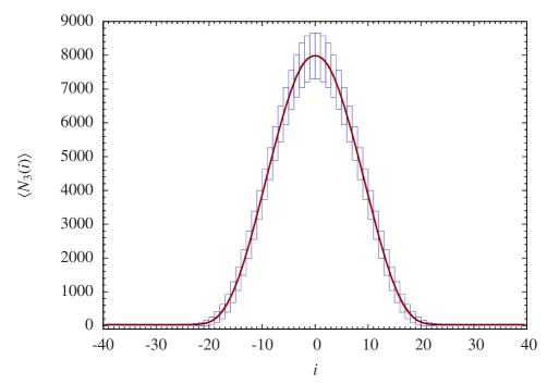
The data shown in Fig. 26 have been collected at the particular values of the bare coupling constants and for (corresponding to ). For these values of we find and have verified relation (220) for ranging from 45.500 to 362.000 building blocks (45.500, 91.000, 181.000 and 362.000). After rescaling the time and volume variables by suitable powers of according to relation (220), and plotting them in the same way as in Fig. 26, one finds almost total agreement between the curves for different spacetime volumes.252525By contrast, the quantum fluctuations indicated in Fig. 26 as vertical bars are volume-dependent. After a rescaling which puts universes of different size on the same curve, the quantum fluctuations will be the larger the smaller the total four-volume, see Sec. 10 below for details. Eq. (220) shows that spatial volumes scale according to and time intervals according to , as one would expect for a genuinely four-dimensional spacetime. This strongly suggests a translation of relation (220) to a continuum notation. The most natural identification is via a proper-time gauge choice
| (225) |
suggested by the CDT setup. With this choice we have
| (226) |
where we have made the identifications
| (227) |
such that
| (228) |
In the second of relations (227), is the constant proportionality factor between the time and genuine continuum proper time , . (The combination contains , related to the four-volume of a four-simplex rather than the three-volume corresponding to a tetrahedron, because its time integral must equal .) Writing , and , eq. (226) is seen to describe a Euclidean de Sitter universe (a four-sphere, the maximally symmetric space for positive cosmological constant) as our searched-for, dynamically generated background geometry! In the parametrization of (226) this is the classical solution to the action
| (229) |
where and is a Lagrange multiplier, fixed by requiring that the total four-volume be , . Up to an overall sign, this is precisely the Einstein-Hilbert action for the scale factor of a homogeneous, isotropic universe [22]
| (230) |
rewritten in terms of the spatial three-volume , although we of course never put any such simplifying symmetry assumptions into the CDT model.
For a fixed, finite four-volume and when applying scaling arguments it can be convenient to rewrite eq. (229) in terms of dimensionless units by introducing and , in which case (229) becomes
| (231) |
now assuming that , and with . A discretized, dimensionless version of (229) is
| (232) |
where . This can be seen by applying the scaling (220), namely, and . With this scaling, the action (232) becomes
| (233) |
where , and therefore has the same form as (231). This enables us to finally conclude that the identifications (227) when used in the action (232) lead naïvely to the continuum expression (229) under the identification
| (234) |
Comparing the kinetic terms in (232) and (229) in more detail,
| (235) |
and using eq. (227) leads to
| (236) |
Eq. (234) now follows from the equations
| (237) |
| (238) |
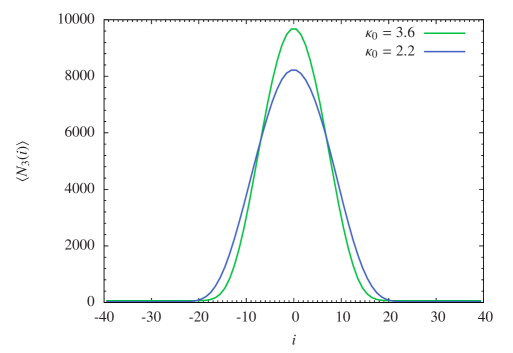
Next, let us comment on the universality of these results. First, we have checked that they are not dependent on the particular definition of time slicing we have been using, in the following sense. By construction of the piecewise linear CDT geometries we have at each integer time step a spatial surface consisting of tetrahedra. Alternatively, one can choose as reference slices for the measurements of the spatial volume non-integer values of time, for example, all time slices at discrete times , . In this case the “triangulation” of the spatial three-spheres consists of tetrahedra – from cutting a (4,1)- or a (1,4)-simplex half-way – and “boxes” (prisms), obtained by cutting a (2,3)- or (3,2)-simplex (as discussed in Sec. 6). We again find a relation like (220) if we use the total number of spatial building blocks in the intermediate slices (tetrahedra+boxes) instead of just the tetrahedra.
Second, we have repeated the measurements for other values of the bare coupling constants. As long as we stay in the phase C well away from the boundaries, a relation like (220) remains valid. In addition, the value of , defined in eq. (220), is almost unchanged until we get close to the phase transition lines beyond which the extended universe disappears. Fig. 27 shows the average shape for and for equal to 2.2 and 3.6. Only for the values of around 3.6 and larger will the measured differ significantly from the value at 2.2. For values larger than 3.8 (at ), we cross the phase transition line between the A and the C phase and the universe will disintegrate into a number of small components distributed along the time axis (as described in detail above), and one can no longer fit the distribution to the formula (220).
Fig. 28 shows the average shape for and equal to 0.2 and 0.6. Here the value is close to the phase transition where the extended universe will flatten out to a universe with a time extension of a few lattice spacings only. Later we will show that while is almost unchanged, the constant in (232), which governs the quantum fluctuations around the mean value , is more sensitive to a change of the bare coupling constants, in particular in the case where we change (while leaving fixed).
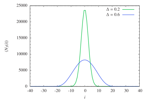
9 Constructive evidence for the effective action
After the first “observations” of the “blob” and measurements which showed that its large-scale behaviour was four-dimensional it was realized that the data were well described by the minisuperspace action (229) (or (230)) [85]. However, only after it was understood how to fix the translational mode did we obtain high-quality data which could provide us with a serious test of the prediction coming from the action (229). While the functional form (220) for the three-volume fits the data perfectly and the corresponding continuum effective action (229) reproduces the continuum version (226) of (220), it is still of interest to check to what extent one can reconstruct the discretized version (232) of the continuum action (229) from the data explicitly. Stated differently, we would like to understand whether there are other effective actions which reproduce the data equally well. As we will demonstrate by explicit construction in this section, there is good evidence for the uniqueness of the action (232).
We have measured two types of data, the three-volume at the discrete time step , and the three-volume correlator . Having created statistically independent configurations by Monte Carlo simulation allows us to construct the average
| (239) |
where the superscript in denotes the result of the k’th configuration sampled, as well as the covariance matrix
| (240) |
Since we have fixed the sum (recall that denotes the fixed number of time steps in a given simulation), the covariance matrix has a zero mode, namely, the constant vector ,
| (241) |
A spectral decomposition of the symmetric covariance matrix gives
| (242) |
where we assume the other eigenvalues of the covariance matrix are different from zero. We now define the “propagator” as the inverse of on the subspace orthogonal to the zero mode , that is,
| (243) |
We now assume we have a discretized action which can be expanded around the expectation value according to
| (244) |
If the quadratic approximation describes the quantum fluctuations around the expectation value well, the inverse of will be a good approximation to the covariance matrix. Conversely, still assuming the quadratic approximation gives a good description of the fluctuations, the constructed from the covariance matrix will to a good approximation allow us to reconstruct the action via (244).
Simply by looking at the inverse of the measured covariance matrix, defined as described above, we observe that it is to a very good approximation small and constant except on the diagonal and the entries next to the diagonal. We can then decompose it into a “kinetic” and a “potential” term. The kinetic part is defined as the matrix with non-zero elements on the diagonal and in the neighbouring entries, such that the sum of the elements in a row or a column is always zero,
| (245) |
where the matrix is given by
| (246) |
Note that the range of lies by definition in the subspace orthogonal to the zero mode. Similarly, we define the potential term as the projection of a diagonal matrix on the subspace orthogonal to the zero mode
| (247) |
The diagonal matrix and the matrices are defined by
| (248) |
and denotes the unit matrix.
The matrix is obtained from the numerical data by inverting the covariance matrix after subtracting the zero mode, as described above. We can now try to find the best values of the and by a least- fit262626A -fit of the form (249) gives the same weight to each three-volume . One might argue that more weight should be given to the larger in a configuration since we are interested in the continuum physics and not in what happens in the stalk where is very small. We have tried various -fits with reasonable weights associated with the three-volumes . The kinetic term, which is the dominant term, is insensitive to any (reasonable) weight associated with . The potential term, which will be analyzed below, is more sensitive to the choice of the weight. However, the general power-law dependence reported below is again unaffected by this choice. to
| (249) |
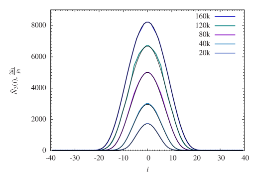
Let us look at the discretized minisuperspace action (232) which obviously has served as an inspiration for the definitions of and . Expanding to second order around one obtains the identifications
| (250) |
where denotes the potential term in (232). We use the fitted coefficients to reconstruct and then compare these reconstructed values with actually measured averages . Similarly, we can use the measured ’s to reconstruct the second derivatives and compare them to the form coming from (232).
The reconstruction of is illustrated in Fig. 29 for a variety of four-volumes and compared with the measured expectation values . One observes that the reconstruction works very well and, most importantly, the coupling constant , which in this way is determined independently for each four-volume is really independent of in the range of considered, as it should.
We will now try to extract the potential from the information contained in the matrix . The determination of is not an easy task as can be understood from Fig. 30, which shows the measured coefficients extracted from the matrix . We consider this figure somewhat remarkable. The interpolated curve makes an abrupt jump by two orders of magnitude going from the extended part of the universe (stretching over roughly 40 time steps) to the stalk. The occurrence of this jump is entirely dynamical, no distinction has ever been made by hand between stalk and bulk.
There are at least two reasons for why it is difficult to determine the potential numerically. Firstly, the results are “contaminated” by the presence of the stalk.
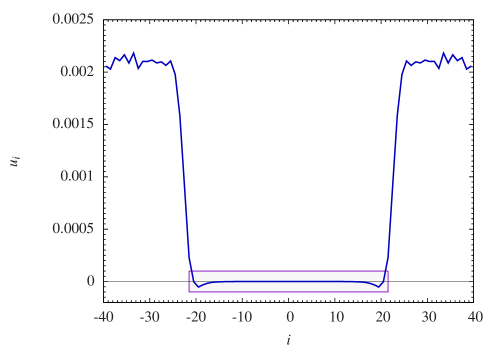
Since it is of cutoff size, its dynamics is dominated by fluctuations which likewise are of cutoff size. They will take the form of short-time subdominant contributions in the correlator matrix . Unfortunately, when we invert to obtain the propagator , the same excitations will correspond to the largest eigenvalues and give a very large contribution. Although the stalk contribution in the matrix is located away from the bulk-diagonal, it can be seen from the appearance of the -term in eqs. (247) and (248) that after the projection orthogonal to the zero mode the contributions from the stalk will also affect the remainder of the geometry in the form of fluctuations around a small constant value. In deriving Fig. 31 we have subtracted this constant value as best possible. However, the fluctuations of the stalk cannot be subtracted and only good statistics can eventually eliminate their effect on the behaviour of the extended part of the quantum universe. The second (and less serious) reason is that from a numerical point of view the potential term is always subdominant to the kinetic term for the individual spacetime histories in the path integral. For instance, consider the simple example of the harmonic oscillator. Its discretized action reads
| (251) |
from which we deduce that the ratio between the kinetic and potential terms will be of order as tends to zero. This reflects the well-known fact that the kinetic term will dominate and go to infinity in the limit as , with a typical path being nowhere differentiable, but closer to a random walk. The same will be true when dealing with a more general action like (229) and its discretized version (232), where scales like . Of course, a classical solution will behave differently: there the kinetic term will be comparable to the potential term. However, when extracting the potential term directly from the data, as we are doing, one is confronted with this issue.

The range of the discrete three-volumes in the extended universe is from several thousand down to five, the kinematically allowed minimum. However, the behaviour for the very small values of near the edge of the extended universe is likely to be mixed in with discretization effects, to be discussed shortly. In order to test whether one really has a -term in the action one should therefore only use values of somewhat larger than five. This has been done in Fig. 31, where we have converted the coefficients from functions of the discrete time steps into functions of the background spatial three-volume using the identification in (250) (the conversion factor can be read off the relevant curve in Fig. 29). It should be emphasized that Fig. 31 is based on data from the extended part of the spacetime only; the variation comes entirely from the central region between times -20 and +20 in Fig. 30, which explains why it has been numerically demanding to extract a good signal. The data presented in Fig. 31 were taken at a discrete volume , and fit well the form , corresponding to a potential . There is a very small residual constant term present in this fit, which presumably is due to the projection onto the space orthogonal to the zero mode, as already discussed earlier. In view of the fact that its value is quite close to the noise level with our present statistics, we have simply chosen to ignore it in the remaining discussion.
Let us finally address the question of how small values of we can use without encountering finite-size effects [96]. Let us consider a universe of size as above. If we are well inside the bulk (more than 6 time steps away from the stalk) we observe a nice Gaussian distribution , where denotes the number of tetrahedra associated to the time-slice at (see Fig. 26 in order to relate the time index to the position of the blob and the position of the stalk). It is peaked around the average value , where the average value with high precision is given by formula (220). A typical measured distribution and a Gaussian fit is shown in Fig. 32.
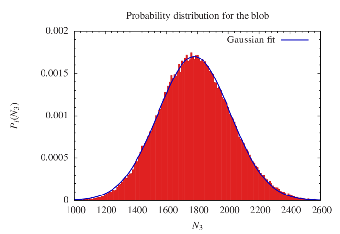
Inside the stalk the situation is very different and we observe pronounced finite-size effects. This is to be expected since we are basically at the cutoff scale. The distribution of three-volumes splits into three separate families. Inside each family the discrete three-volumes differ by 3, such that we have three sets of possible -values, , and . When we start to move from the stalk and into the bulk, some memory of this will remain for small , as shown in Fig. 33. The bulk distribution of Fig. 26 extends over approximately 42 lattice spacings in the time direction. For distances up to six lattice spacings from the “boundary” between the stalk and bulk (on both sides) one can observe phenomena like those shown in Fig. 33, which of course are most pronounced close to the boundary. The figure shows the distribution of three-volume at five time steps from the “boundary” between the stalk and the bulk (see Fig. 26 for the position of bulk and stalk). For small one observes the split into three distributions, which for merge into one. However, even then the picture is quite different from the Gaussian distribution far away from the stalk, shown in Fig. 32.
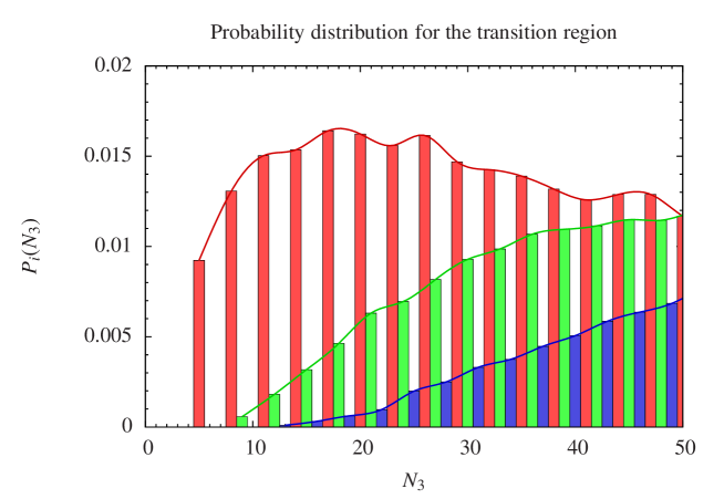
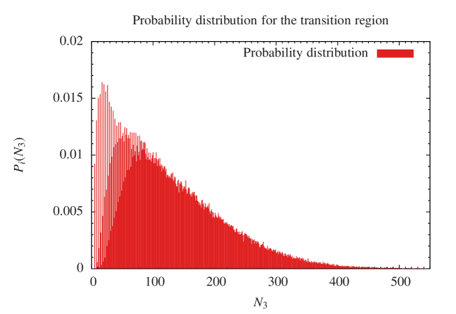
When we consider for , the chance of finding a sufficiently small to observe the finite-size effects just mentioned is essentially zero. From Fig. 31 it is clear that the real test of the power law requires small , but we cannot use for the reasons just stated. A fair way to state our result is that the data are consistent with a law, as seen from Fig. 31. On the other hand, if one performs a fit to determine the power 5/3, the error bars will be quite large.
Apart from obtaining the correct power law for the potential for a given spacetime volume , it is equally important that the coefficient in front of this term be independent of . This seems to be the case as is shown in Fig. 34, where we have plotted the measured potentials in terms of reduced, dimensionless variables which make the comparison between measurements for different easier.
In summary, we conclude that the data allow us to reconstruct the action (232) with good precision. Quantifying the short-distance artifacts for one quantity gives us a good idea of the scale at which they occur for a given four-volume, but still leaves us with the difficulty of disentangling them from genuine quantum-gravity signatures in this and other observables. For example, the non-Gaussian character of the distribution of fluctuations around the sphere (220) at small observed above could indicate new short-distance physics, say, along the lines suggested in the asymptotic safety scenario [97]. We presently do not know how to relate the deviation from the four-sphere at a small scale factor described there to our explicit small- “observations”, but it would clearly be interesting to do so.

9.1 Relation to Hořava-Lifshitz gravity (part II)
As described above our data in phase C fits well to (232), the discretized version of the minisuperspace action (229). However, there is a residual ambiguity in the interpretation of the time coordinate, as it appears in the identification (227), which takes the form of an overall, finite scaling between time and spatial directions. As we have emphasized a number of times, due to the entropic nature of the effective action, there is no compelling reason to take the microscopic geometric length assignments literally. We have chosen the time “coordinate” such that we obtain a round four-sphere. However, the shape of the universe clearly changes in terms of the number of lattice spacings in time direction relative to those in the spatial directions when we vary the bare coupling constants and . Although this change is qualitatively in agreement with the change of as a function of and (recall eqs. (2.9.3) and (73) which define and , as well as Fig. 2), there is no detailed quantitative agreement, as we have already mentioned. Thus, rather than choosing time to be consistent with an -geometry, an alternative interpretation at this stage is to assume that the effective action is changing. Since the CDT set-up allows us to refer to its distinguished time slicing, a deformation à la Hořava-Lifshitz suggests itself. A corresponding effective Euclidean continuum action, including the measure, and expressed in terms of standard metric variables could be of the form
| (252) |
where denotes the extrinsic curvature, the three-metric on the spatial slices, the corresponding three-dimensional scalar curvature, the lapse function, and finally a “potential” which in Hořava’s continuum formulation would contain higher orders of spatial derivatives, potentially rendering renormalizable. In our case we are not committed to any particular choice of potential , since we are not imposing renormalizability of the theory in any conventional sense. An effective could be generated by entropy, i.e. by the measure, and may not relate to any discussion of the theory being renormalizable. The kinetic term depending on the extrinsic curvature is the most general such term which is at most second order in time derivatives and consistent with spatial diffeomorphism invariance. The parameter appears in the (generalized) DeWitt metric, which defines an ultralocal metric on the classical space of all three-metrics.272727The value of governs the signature of the generalized DeWitt metric which is positive definite for , indefinite for and negative definite for . The role of in three-dimensional CDT quantum gravity has been analyzed in detail in [98]. The parameter can be related to a relative scaling between time and spatial directions. When and we recover the standard (Euclidean) Einstein-Hilbert action.
Making a simple minisuperspace ansatz with compact spherical slices, which assumes homogeneity and isotropy of the spatial three-metric , and fixing the lapse to , the Euclidean action (252) becomes a function of the scale factor (see also [99, 100, 101]), that is,
| (253) |
The first three terms in the parentheses define the IR limit, while the potential term contains inverse powers of the scale factor coming from possible higher-order spatial derivative terms.
Our reconstruction of the effective action from the computer data, as described above, is compatible with the functional form of the minisuperspace action (253). Importantly, we so far have not been able to determine the constant in front of the potential term in (233) with any precision, which would enable us to fix the ratio appearing in (253). Also, as we have already discussed, it is presently not possible to determine , which could be important for small values of the scale factor. Once we have developed a better computer algorithm which allows us to approach the B-C phase transition line, testing such Hořava-Lifshitz scenarios will hopefully become easier.
9.2 Some preliminary conclusions
Let us emphasize a remarkable aspect of our results. Our starting point was the Regge action for CDT, as described in Sec. 2 above. However, the effective action we have generated dynamically by performing the nonperturbative sum over histories is only indirectly related to this “bare” action. Likewise, the coupling constant which appears in front of the effective action, and which we view as related to the gravitational coupling constant by eq. (234), has no obvious direct relation to the “bare” coupling appearing in the Regge action (73). Nevertheless the leading terms in the effective action for the scale factor are precisely the ones presented in (229) or, more generally, in the effective Hořava-type action (253). The fact that a kinetic term with a second-order derivative appears as the leading term in an effective action is perhaps less surprising, but that it has precisely the form (229) or (253), including the term , is remarkable and very encouraging for the entire CDT quantization program. Until now our results are compatible with the Einstein-Hilbert action, but better data are required to discriminate between the actions (229) and (253). In general, solutions to the more general action (253) will be stretched spheres [102], which have conical singularities at the end points (in our case the locations where the stalk starts). However, these singularities in the curvature will not be visible in the observable .
10 Fluctuations around de Sitter space
We have shown that the action (232) gives an excellent description of the measured shape of the extended universe. Assuming that the three-volume fluctuations around are sufficiently small so that a quadratic approximation is valid, we have also shown that we can use the measured fluctuations to reconstruct the discretized version (232) of the minisuperspace action (229), where and are independent of the total four-volume used in the simulations. This certainly provides strong evidence that both the minisuperspace description of the dynamical behaviour of the (expectation value of the) three-volume, and the semiclassical quadratic truncation for the description of the quantum fluctuations in the three-volume are essentially correct.
In the following we will test in more detail how well the actions (229) and (232) describe the data encoded in the covariance matrix .
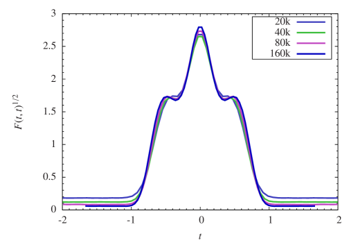
The correlation function was defined in the previous section by
| (254) |
where we have included an additional subscript to emphasize that is kept constant in a given simulation. The first observation extracted from the Monte Carlo simulations is that under a change in the four-volume scales as282828We stress again that the form (255) is only valid in that part of the universe whose spatial extension is considerably larger than the minimal constructed from five tetrahedra. (The spatial volume of the stalk typically fluctuates between five and fifteen tetrahedra.)
| (255) |
where is a universal scaling function. This is illustrated by Fig. 35 for the rescaled version of the diagonal part , corresponding precisely to the quantum fluctuations of Fig. 26. While the height of the curve in Fig. 26 will grow as , the superimposed fluctuations will only grow as . We conclude that for fixed bare coupling constants the relative fluctuations will go to zero in the infinite-volume limit .
From the way the factor appears as an overall scale in eq. (233) it is clear that to the extent a quadratic expansion around the effective background geometry is valid one will have a scaling
| (256) |
where . This implies that (255) provides additional evidence for the validity of the quadratic approximation and the fact that our choice of action (232), with independent of , is indeed consistent.
To demonstrate in detail that the full function and not only its diagonal part is described by the effective actions (229), (232), let us for convenience adopt a continuum language and compute its expected behaviour. Expanding (229) around the classical solution according to , the quadratic fluctuations are given by
| (257) | |||||
where is the normalized measure and the quadratic form is determined by expanding the effective action to second order in ,
| (258) |
In expression (258), denotes the Hermitian operator
| (259) |
which must be diagonalized under the constraint that , since is kept constant.
Let be the eigenfunctions of the quadratic form given by (258) with the volume constraint enforced292929One simple way to find the eigenvalues and eigenfunctions approximately, including the constraint, is to discretize the differential operator, imposing that the (discretized) eigenfunctions vanish at the boundaries and finally adding the constraint as a term to the action, where the coefficient is taken large. The differential operator then becomes an ordinary matrix whose eigenvalues and eigenvectors can be found numerically. Stability with respect to subdivision and choice of is easily checked., ordered according to increasing eigenvalues . As we will discuss shortly, the lowest eigenvalue is , associated with translational invariance in time direction, and should be left out when we invert , because we precisely fix the centre of volume when making our measurements. Its dynamics is therefore not accounted for in the correlator .
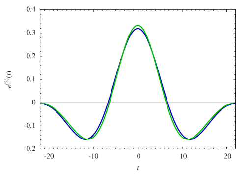
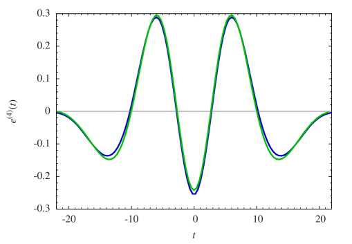
If this cosmological continuum model were to give the correct description of the computer-generated universe, the matrix
| (260) |
should be proportional to the measured correlator . Fig. 36 shows the eigenfunctions and (with two and four zeros respectively), calculated from with the constraint imposed. Simultaneously we show the corresponding eigenfunctions calculated from the data, i.e. from the matrix , which correspond to the (normalizable) eigenfunctions with the highest and third-highest eigenvalues. The agreement is very good, in particular when taking into consideration that no parameter has been adjusted in the action (we simply take in (226) and (258), which for gives , where denotes the time distance between successive slices).
The reader may wonder why the first eigenfunction exhibited has two zeros. As one would expect, the ground state eigenfunction of the Hamiltonian (259), corresponding to the lowest eigenvalue, has no zeros, but does not satisfy the volume constraint . The eigenfunction of with next-lowest eigenvalue has one zero and is given by the simple analytic function
| (261) |
where is a constant. One realizes immediately that is the translational zero mode of the classical solution (). Since the action is invariant under time translations we have
| (262) |
and since is a solution to the classical equations of motion we find to second order (using the definition (261))
| (263) |
consistent with having eigenvalue zero.
It is clear from Fig. 36 that some of the eigenfunctions of (with the volume constraint imposed) agree very well with the measured eigenfunctions. All even eigenfunctions (those symmetric with respect to reflection about the symmetry axis located at the centre of volume) turn out to agree very well. The odd eigenfunctions of agree less well with the eigenfunctions calculated from the measured . The reason seems to be that we have not managed to eliminate the motion of the centre of volume completely from our measurements. As already mentioned above, there is an inherent ambiguity in fixing the centre of volume, which turns out to be sufficient to reintroduce the zero mode in the data. Suppose we had by mistake misplaced the centre of volume by a small distance . This would introduce a modification
| (264) |
proportional to the zero mode of the potential . It follows that the zero mode can re-enter whenever we have an ambiguity in the position of the centre of volume. In fact, we have found that the first odd eigenfunction extracted from the data can be perfectly described by a linear combination of and . It may be surprising at first that an ambiguity of one lattice spacing can introduce a significant mixing. However, if we translate from eq. (264) to “discretized” dimensionless units using , we find that , which because of is of the same order of magnitude as the fluctuations themselves. In our case, this apparently does affect the odd eigenfunctions.
11 The size of the universe
Let us now return to equation (234),
| (265) |
which relates the parameter extracted from the Monte Carlo simulations to Newton’s constant in units of the cutoff , . For the bare coupling constants we have high-statistics measurements for ranging from 45.500 to 362.000 four-simplices (equivalently, ranging from 20.000 to 160.000 four-simplices). The choice of determines the asymmetry parameter , and the choice of determines the ratio between and . This in turn determines the “effective” four-volume of an average four-simplex, which also appears in (265). The number in (265) is determined directly from the time extension of the extended universe according to
| (266) |
Finally, from our measurements we have determined . Taking everything together according to (265), we obtain , or , where is the Planck length.
From the identification of the volume of the four-sphere, , we obtain that . In other words, the linear size of the quantum de Sitter universes studied here lies in the range of 12-21 Planck lengths for in the range mentioned above and for the bare coupling constants chosen as .
Our dynamically generated universes are therefore not very big, and the quantum fluctuations around their average shape are large as is apparent from Fig. 26. It is rather surprising that the semiclassical minisuperspace formulation is applicable for universes of such a small size, a fact that should be welcome news to anyone performing semiclassical calculations to describe the behaviour of the early universe. However, in a certain sense our lattices are still coarse compared to the Planck scale because the Planck length is roughly half a lattice spacing. If we are after a theory of quantum gravity valid on all scales, we are in particular interested in uncovering phenomena associated with Planck-scale physics. In order to collect data free from unphysical short-distance lattice artifacts at this scale, we would ideally like to work with a lattice spacing much smaller than the Planck length, while still being able to set by hand the physical volume of the universe studied on the computer.
The way to achieve this, under the assumption that the coupling constant of formula (265) is indeed a true measure of the gravitational coupling constant, is as follows. We are free to vary the discrete four-volume and the bare coupling constants of the Regge action. Assuming for the moment that the semiclassical minisuperspace action is valid, the effective coupling constant in front of it will be a function of the bare coupling constants , and can in principle be determined as described above for the case . If we adjusted the bare coupling constants such that in the limit as both
| (267) |
remained constant (i.e. ), we would eventually reach a region where the lattice spacing was significantly smaller than the Planck length, in which event the lattice could be used to approximate spacetime structures of Planckian size and we could initiate a genuine study of the sub-Planckian regime.
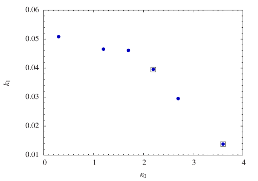
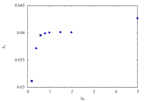
Since we have no control over the effective coupling constant , the first obvious question which arises is whether we can at all adjust the bare coupling constants in such a way that at large scales we still see a four-dimensional universe, with going to zero at the same time. The answer seems to be in the affirmative, as we will now go on to explain.
Fig. 37 shows the results of extracting for a range of bare coupling constants for which we still observe an extended universe. In the top figure is kept constant while is varied. For sufficiently large we eventually reach a point where the A-C transition takes place (the point in the square in the bottom right-hand corner is the measurement closest to the transition we have looked at). For even larger values of , beyond this transition, the universe disintegrates into a number of small universes, in a CDT-analogue of the branched-polymer phase of Euclidean quantum gravity, as described above. The plot shows that the effective coupling constant becomes smaller and possibly goes to zero as the phase transition point is approached, although our current data do not yet allow us to conclude that does indeed vanish at the transition point.
Conversely, the bottom figure of Fig. 37 shows the effect of varying , while keeping fixed. As is decreased from 0.6, we eventually hit the B-C phase transition, separating the physical phase of extended universes from the CDT-equivalent of the crumpled phase of Euclidean quantum gravity, where the entire universe will be concentrated within a few time steps. Strictly speaking we are not able to go much closer than to , as already explained. It seems that the effective coupling constant starts to decrease in value when is decreasing from 0.6, but since we cannot get very close to the phase boundary, we cannot in any convincing way say that along the B-C phase boundary.
To extract the coupling constant from (265) we not only have to take into account the change in , but also that in (the width of the distribution ) and in the effective four-volume as a function of the bare coupling constants. Combining these changes, we arrive at a slightly different picture. Approaching the B-C boundary the gravitational coupling constant does not vary much, despite the fact that increases. This is a consequence of decreasing considerably, as can be seen from Fig. 28. On the other hand, when we approach the A-C the effective gravitational coupling constant increases, more or less like , where the behaviour of is shown in Fig. 37 (left). This implies that the Planck length increases from approximately to when changes from 2.2 to 3.6. On the basis of these arguments it seems that we have to go very close to the phase boundaries in order to penetrate into the sub-Planckian regime.
One interesting issue under investigation is whether and to what extent the simple minisuperspace description remains valid as we go to shorter scales. This raises the interesting possibility of being able to test explicitly the scaling violations of predicted by renormalization group methods in the context of asymptotic safety [5]. We will discuss this in detail in Sec. 13.
12 The fractal dimensions
12.1 The spectral dimension
One way to obtain information about the geometry of our quantum universe is by studying a diffusion process on the underlying geometric ensemble. We will use this technique to determine the so-called spectral dimension of the ensemble of geometries.
As a start let us discuss briefly diffusion on a -dimensional manifold with a fixed, smooth Riemannian metric . The diffusion equation has the form
| (268) |
where is a fictitious diffusion time, the Laplace operator of the metric and the probability density of diffusion from to in diffusion time . We will consider diffusion processes which initially are peaked at some point ,
| (269) |
For the special case of a flat Euclidean metric, we have
| (270) |
For general curved spaces has the well-known asymptotic expansion
| (271) |
for small , where denotes the geodesic distance between and . Note the appearance of the power in this relation, reflecting the dimension of the manifold, just like in the formula (270) for flat space. This happens because small values of correspond to short distances and for any given smooth metric short distances imply approximate flatness.
A quantity that is easier to measure in numerical simulations is the average return probability , which possesses an analogous expansion for small ,
| (272) |
where is the spacetime volume and the expansion coefficients are given by
| (273) |
For an infinite flat space, we have and thus can extract the dimension by taking the logarithmic derivative,
| (274) |
independent of . For non-flat spaces and/or finite volume , one can still use eq. (274) to extract the dimension, but there will be corrections for sufficiently large . For finite volume in particular, goes to for since the zero mode of the Laplacian will dominate the diffusion in this region. For a given diffusion time the behaviour of is determined by eigenvalues of with , and the contribution from higher eigenvalues is exponentially suppressed. Like in the flat case, where diffusion over a time probes the geometry at a linear scale , large corresponds to large distances away from the origin of the diffusion process, and small to short distances.
The construction above can be illustrated by the simplest example of diffusion in one dimension. The solution to the diffusion equation on the real axis, starting at the origin, is
| (275) |
where denotes the Fourier transform of . The eigenvalues of the Laplace operator are of course just given by . In order to illustrate the finite-volume effect, let us compactify the real line to a circle of length . The return probability is now given by
| (276) |
where in the second step we have performed a Poisson resummation to highlight the -dependence for small . In line with the discussion above, the associated spectral dimension is constant (and equal to one) up to -values of the order , and then goes to zero monotonically.
In applying this set-up to four-dimensional quantum gravity in a path integral formulation, we are interested in measuring the expectation value of the return probability . Since defined in (272) is invariant under reparametrizations, it makes sense to take its quantum average over all geometries of a given spacetime volume ,
| (277) |
in accordance with the definition of expectation values (209). Since the small- behaviour of is the same for each smooth geometry, it might seem obvious that the same is true for their integral , but this need not be so. Firstly, the scale in (277) is held fixed, independent of the geometry , while the expansion (272) contains reference to higher powers of the curvature of . Secondly, one should keep in mind that a typical geometry which contributes to the path integral – although continuous – is unlikely to be smooth. This does not invalidate our treatment, since diffusion processes can be meaningfully defined on much more general objects than smooth manifolds. For example, the return probability for diffusion on fractal structures is well studied in statistical physics and takes the form
| (278) |
where is the “volume” associated with the fractal structure and the so-called spectral dimension, which is not necessarily an integer. An example of fractal structures are branched polymers which generically have [103, 104]. Extensive numerical simulations [105, 106] have shown that in two-dimensional quantum gravity the only effect of integrating over geometries is to replace the asymptotic expansion (272), which contains reference to powers of the curvature related to a specific metric, by the simpler form (278).
Our next task is to define diffusion on the class of metric spaces under consideration, the piecewise linear structures defined by the causal triangulations . At this point we will cheat a little. When translating eq. (268) into a form suitable for our piecewise linear geometries we will assume , although this is strictly speaking not the case. The motivation is that the expression for is more complicated, and that following the diffusion on large triangulations consumes a lot of computer time. Since we are presently only trying to determine which is a reasonably universal exponent, we expect it to be independent of the exact discretized implementation of the Laplacian on the piecewise linear geometry.
We start from an initial probability distribution
| (279) |
which vanishes everywhere except at a randomly chosen (4,1)-simplex , and define the diffusion process by the evolution rule
| (280) |
These equations are the simplicial analogues of (269) and (268), with the triangulation (together with its Euclideanized edge-length assignments) playing the role of , and denoting the five nearest neighbours of the four-simplex . Clearly (280) is only the discretized Laplacian if the length assignments of all links is 1 (in lattice units), i.e. , as just discussed. In this process, the total probability
| (281) |
is conserved. The return probability to a simplex is then defined as and the quantum average as
| (282) |
where denotes a triangulation with four-simplices, and and are the obvious simplicial analogues of the continuum quantities at fixed four-volume. Assuming that the return probability behaves according to (278), with , we can extract the value of the fractal dimension by measuring the logarithmic derivative as in (274) above, as long as the diffusion time is not much larger than ,
| (283) |
From the experience with numerical simulations of two-dimensional Euclidean quantum gravity in terms of dynamical triangulations [107, 105, 106], we expect some irregularities in the behaviour of the return probability for the smallest , i.e. close to the cutoff scale. Typically, the behaviour of for odd and even diffusion steps will be quite different for small and merge only for . After the merger, the curve enters a long and stable regime where the right-hand side of (283) is independent of , before finite-size effects start to dominate which force it to go to zero.
The origin of the odd-even asymmetry can again be illustrated by the simple case of diffusion on a circle, whose solution is the discretized version of the solution (276). In this case the asymmetry of the return probability between odd and even time steps is extreme: if we use the one-dimensional version of the simple evolution equation (280), we obtain
| (284) |
as long as , where is the discrete volume of the circle (i.e. the number of its edges). It is of course possible to eliminate this asymmetry by using an “improved” discretized diffusion equation, but in the case of higher-dimensional random geometries like those used in four-dimensional causal dynamical triangulations this is not really necessary.
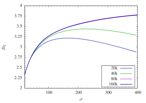
The results of measuring the spacetime spectral dimension were first reported in [108] and discussed in detail in [78]. We work with system sizes of up to k with , and . Since we are interested in the bulk properties of quantum spacetime and since the volume is not distributed evenly in the time direction (cf. Fig. 20), we always start the diffusion process from a four-simplex adjacent to the slice of maximal three-volume. When this is done the variations in the curve for different generic choices of triangulation and starting simplices are small. The data curves presented in Fig. 38 were obtained by averaging over 400 different diffusion processes performed on independent configurations. We have omitted error bars from Fig. 38 to illustrate how the curves converge to a shape that represents in the infinite-volume limit, and which is given by the envelope of the data curves for finite volume. For the two lower volumes, k and k, there still are clear finite-volume effects for large diffusion times .
By contrast, the top curve – corresponding to the maximal volume k – continues to rise for increasing , which makes it plausible that we can ignore any finite-size effects and that it is a good representative of the infinite-volume limit in the -range considered.303030In both Figs. 38 and 39 we have only plotted the region where the curves for odd and even coincide, in order to exclude short-distance lattice artifacts. The two curves merge at about . Since the diffusion distance grows as , a return diffusion time of 40 corresponds to just a few steps away from the initial four-simplex. We will therefore concentrate on analyzing the shape of this curve, which is presented separately in Fig. 39, now with error bars included. (More precisely, the two outer curves represent the envelopes to the tops and bottoms of the error bars.) The error grows linearly with , due to the occurrence of the log in (283).
The remarkable feature of the curve is its slow approach to the asymptotic value of for large . This type of behaviour has never been observed previously in systems of random geometry (see e.g. [107, 105, 109]), and again underlines that causal dynamical triangulations in four dimensions behave qualitatively differently, and that the quantum geometry produced is in general richer. The new phenomenon we observe here is a scale dependence of the spectral dimension, which has emerged dynamically. This is to be contrasted with fractal structures which show a self-similar behaviour at all scales.
A best three-parameter fit which asymptotically approaches a constant is of the form
| (285) |
The constants , and have been determined by using the full data range and the curve shape agrees well with the measurements, as can be seen from Fig. 39. Integrating (285) we obtain
| (286) |
from which we deduce the limiting cases
| (287) |
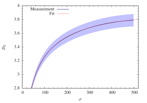
We conclude that the quantum geometry generated by causal dynamical triangulations has a scale-dependent spectral dimension which increases continuously from to with increasing distance. Substituting the values for , and obtained from the fit (285), and taking into account their variation as we vary the -range and use different weightings for the errors, we obtained the asymptotic values [108, 78]
| (288) |
for the “long-distance spectral dimension” and
| (289) |
for the “short-distance spectral dimension”.
A dynamically generated scale-dependent dimension with this behaviour signals the existence of an effective ultraviolet cutoff for theories of gravity, brought about by the (highly nonperturbative) behaviour of the quantum-geometric degrees of freedom on the very smallest scale. Of course, one should not lose sight of the fact that this is a numerical result, based on data and fits. It would be desirable to have a model which exhibits a scale-dependent spectral dimension and can be understood analytically, in order to illuminate the mechanism at work in CDT quantum gravity. An example of such a model has been constructed recently [110].
After we observed the dynamical reduction (to ) of the spectral dimension at short distances, there has been a considerable amount of theoretical work showing that in the UV regime comes about naturally also in the asymptotic safety scenario [97], in Hořava-Lifshitz gravity [111] and even more generally [112]. Comparative studies of the behaviour of the spectral dimension away from the asymptotic UV and IR regimes have been conducted in [113]. In the next section we will discuss how one can imagine making contact with these other theories of quantum gravity and also why the UV spectral dimension in these theories is equal to 2.
Finally, it should be mentioned that the observed short-distance value agrees within measuring accuracy with old measurements of the spectral dimension in Euclidean DT quantum gravity in the so-called “crinkled” phase [114]. This phase was “discovered” when a number of gauge fields were coupled to Euclidean four-dimensional gravity using the formalism of dynamical triangulations. The effect of the gauge fields is to change the typical geometry from branched-polymer type with Hausdorff dimension 2 and spectral dimension 4/3 to a different type of geometry with Hausdorff dimension close to 4 and a spectral dimension . It was shown subsequently that one can obtain the same geometric results by forgetting about the -gauge fields altogether and instead assigning an additional weight to each triangulation , where denotes a triangle in and is the order of , i.e. the number of four-simplices to which belongs. For suitable values of one could reproduce most of the geometric features resulting from the addition of -gauge fields [115]. Since the Regge curvature is located at the triangles and – when using identical building blocks like in DT – only depends on the order of , it was natural to view the weight as an effective higher-order curvature term in the action, resulting from integrating out the gauge fields. However, this otherwise appealing interpretation was somewhat undermined by the observation that precisely this weight factor arises when changing the assignment of the -gauge field from the links to the dual links [116], suggesting that one is dealing merely with discretization ambiguities, which are unlikely to leave an imprint in the continuum limit. The conclusion at the time was that the crinkled phase, just like the other phases in pure, four-dimensional Euclidean DT, is a lattice artifact. Nevertheless, the crinkled phase was reconsidered recently in [117], where the spectral dimension was measured again and found to be in agreement with the old results obtained in [114, 115]. At the same time it was noticed that it displays a scale-dependence similar to that observed in four-dimensional CDT. If other physically desirable features can be shown to be present in this phase, it may mean that there is a truly isotropic model which belongs to the same universality class as CDT. This is an interesting suggestion which deserves further study.
In closing, let us remark that – apart from allowing us to define and measure the spectral dimension – the diffusion equation is an immensely useful tool for studying the geometry of quantum space. A lot of interesting work has been reported, both in three- [102] and four-dimensional CDT [86], related to the more detailed shape of the computer-generated quantum universes.
12.2 The Hausdorff dimension
The diffusion equation probes certain aspects of the underlying spacetime, which – important for our purposes – extend into the quantum regime, as we have seen above. For smooth manifolds the spectral dimension defined from the diffusion equation agrees with the ordinary, topological dimension of the manifold and its so-called Hausdorff dimension. For fractal geometries, like those encountered in the path integral, the Hausdorff dimension can differ from the spectral dimension, while there may be no “ordinary” dimension. Here we will define and measure the Hausdorff dimension both for a spatial slice and for the entire spacetime between two spatial slices. Let us start with a spatial slice of a given configuration of spacetime as it appears in the path integral. Due to the presence of a time foliation we have well-defined spatial slices with the topology of three-spheres at discretized times , constructed by gluing together tetrahedra.
Our algorithm for determining the Hausdorff dimension of the spatial slices is as follows. From a given time slice of discrete volume , we randomly pick a tetrahedron . From , we move out by one step and obtain tetrahedra at distance 1 from (that is, its nearest neighbours). Moving out by a further step, there will be tetrahedra at distance 2, and so on until all tetrahedra have been visited. The numbers recorded for each (discrete) distance sum up to
| (290) |
Finally, we measure the average linear extension
| (291) |
of the spatial slice. For a slice of volume , this process is repeated times with different randomly chosen initial tetrahedra. The expectation value is then averaged over these measurements. In this way, we obtain for every slice a data pair
| (292) |
representing one “bare” measurement.
This process is performed for all spatial slices of the given geometry. We have typically done this for about 1000 different spacetime geometries. The final results are sorted by their -value (in practice a continuous variable) and averaged over a sequence of 100 consecutive points. The data points are then displayed on a log-log plot. In the presence of finite-size scaling, we expect them to follow a curve
| (293) |
defining a spatial Hausdorff dimension . Our results, which show universal behaviour and scaling, are presented in Fig. 40.
\psfrag{log2}{\bf{\Large$\log\langle r\rangle$}}\psfrag{log1}{\Large\bf$\log\langle N_{3}\rangle$}\includegraphics{haus2.2b4.ps}
Another substructure of spacetime whose geometry can be investigated straightforwardly are what we shall call “thick” spatial slices, namely, the sandwiches of geometry contained in between two adjacent spatial slices of integer times and , with topology . Such thick spatial slices are made up of four-simplices of types (4,1) and (3,2) and their time-reversed counterparts (1,4) and (2,3). To determine the Hausdorff dimension of the thick slices, we pick a random four-simplex from such a slice. We proceed then exactly as we did when measuring the Hausdorff dimension of the spatial slices at integer-. Starting from the randomly chosen initial four-simplex, we move out, one step at a time, to the nearest neighbours at distance , from the previous set of building blocks at distance , except that we never allow the crossing of the time slices and . At each step, we keep track of the number of building blocks, whose sum is equal to the total slice volume ,
| (294) |
which enables us to compute the average linear size
| (295) |
of the thick slice. For a given slice of volume , this process is then repeated times with randomly chosen initial building blocks. The average size is again averaged over this set and the data pair stored. Using the same procedure as described following formula (292) above, we extract the Hausdorff dimension from the relation
| (296) |
The results are presented in Fig. 41 in the form of a log-log plot.
\psfrag{log1}{\bf{\Large$\log\langle r\rangle$}}\psfrag{log2}{\Large\bf$\log\langle N\rangle$}\includegraphics{Haus2.2b6.ps}
The straight line corresponds to , and the best fitted value is . Measurements were performed on spacetimes with total size 20, 40 and 80k, at , . – We conclude that the transition from a genuine constant-time slice to a thick slice adds one extra dimension to the Hausdorff dimension – the thickened slice already “feels” some aspects of the four-dimensionality of the full spacetime. Note that this would not be true for a thick slice of a classical, regular lattice, whose Hausdorff dimension would be the same as that of a “thin” slice. The likely mechanism for the dimensional increase in the triangulations is the appearance of “short-cuts” between two tetrahedral building blocks, say, once one moves slightly away from a slice of integer-. Finally, it is also true that if we simply measure the Hausdorff dimension without any restriction to stay within a “thick” spatial slice we still obtain .
13 Making contact with asymptotic safety
As we discussed earlier, it is technically challenging to get close to the B-C phase transition line, which is needed if we want to achieve a higher resolution in the UV regime, such that the lattice spacing is much smaller than the Planck length. Also, we do not know yet whether in such a limit we have an isotropic scaling behaviour in space and time, like in the asymptotic safety approach, or need to invoke a more general, anisotropic scenario as outlined above. For the time being, let us assume that the end point of the B-C transition line in the phase diagram of Fig. 17 corresponds to an isotropic phase transition point. How can one make contact with the gravitational renormalization group treatment? The standard way would be to “measure” observables (by lattice Monte Carlo simulations), like a mass in QCD or the string tension in Yang-Mills theory. For definiteness, let us consider the string tension , which has mass dimension two. The measurements, for some choice of the bare coupling constant, will give us a number . We now write
| (297) |
where is the dimensionful, physical string tension and describes the dependence of the lattice spacing on the bare coupling constant . Similarly, one can try to measure the mass of the glueball, which on the lattice will be some number . The relation analogous to (297) is
| (298) |
where is the physical glueball mass. Being able to write down relations like this for all observables, where is determined by the renormalization group equation
| (299) |
allows us to define a continuum theory at a fixed point where , since there we can take when . In the case of QCD or Yang-Mills theory the fixed point is the Gaussian fixed point , but in the more general setting of asymptotic safety it will be non-Gaussian.
Assume now that we have a fixed point for gravity. The gravitational coupling constant is dimensionful, and we can write for the bare coupling constant
| (300) |
The IR fixed point corresponds to constant while the putative non-Gaussian fixed point corresponds to , i.e. . In our case it is tempting to identify our dimensionless constant with , up to the constant of proportionality given in (234). Close to the UV fixed point we have
| (301) |
Usually one relates the lattice spacing near the fixed point to the bare coupling constants with the help of some correlation length . Assume that diverges according to
| (302) |
in the limit as we tune the bare coupling constant . This correlation length is associated with a field correlator and usually some physical mass (like the glue-ball mass referred to in (298)) by means of
| (303) |
where is a discrete lattice distance and a physical distance. Requiring the physical quantities and to remain constant as then fixes as a function of the bare coupling constant,
| (304) |
Eq. (304) is only valid close to the fixed point and should be compared to the renormalization group equation (299), from which we deduce that .
In the gravitational case at hand we do not (yet) have observables which would allow us to define meaningful correlation lengths. At any rate, it is by no means a settled issue how to define such a concept in a theory where one integrates over all geometries, and where the length is itself a function of geometry, as already emphasized in the Introduction (see [15] for related discussions). Instead, we construct from our computer-generated “data” an effective action, where all degrees of freedom, apart from the scale factor, have been integrated out. We impose the constraint that the data are fitted to a universe of total lattice four-volume . Measurements are performed at different, fixed values of , all the while maintaining the relation313131In principle, we should be taking into account the different volumes of the two types of four-simplices, which depend on , but we will ignore these details to streamline the presentation.
| (305) |
We then “remove the regulator” by investigating the limit . In ordinary lattice field theory, we have two options for changing ; either we keep fixed, and therefore change , or we keep fixed and change . Let us illustrate the difference in terms of a scalar field on a lattice. Its dimensionless action can be written as
| (306) |
where labels discrete lattice points and unit vectors in the different lattice directions. The correlation length is approximately lattice spacings. Holding fixed and increasing is not going to change the correlation length in any significant way if is sufficiently large. Thus the interpretation for fixed is straightforward: the physical volume is simply increased and finite-size effects will become smaller and smaller. However, we can also insist on an interpretation where is kept fixed, is increased and decreased accordingly. In this case, the lattice becomes finer and finer with increasing . But now the physical interpretation of (306) will change with increasing , even if no bare coupling constant is changed, and the correlation length is still approximately lattice spacings. Since the physical lattice length decreases proportional to the physical correlation length is going to zero, and the physical mass to infinity. This can be made explicit in (306) by introducing the lattice spacing ,
| (307) |
The physical mass is and goes to infinity unless we adjust . The factor in front of the sum can be reabsorbed in a redefinition of if desired.
In our case it is natural to consider as fixed if we want to make contact with the continuum framework of asymptotic safety, since this will allow us to vary . However, like in the ordinary field theory case just discussed, it requires the fine-tuning of some coupling constants to consider as fixed when . In the free field case we had to fine-tune the bare mass to zero as . In the gravity case the need for a fine-tuning of some kind is also clear if we consider Fig. 26. The bars indicated in the figure refer to a specific spacetime four-volume which we label by , without any reference to . For a given choice of bare coupling constants the size of the bars reflects real fluctuations of the three-volumes of our quantum universe. When increases, but the bare coupling constants are kept fixed, we saw that the relative size of the fluctuations went to zero. This is an indication that we should view as going to infinity when . It is natural to assume that if we want to have the physics associated with the continuum volume (approximately) invariant when , the relative fluctuations of must be constant as a function of . This is only possible by changing the bare coupling constants. As discussed above, it is not a foregone conclusion that this can be achieved. For instance, we may have to enlarge the coupling constant space to also include the fluctuations of (and thus only talk about , and not ), i.e. reintroduce the cosmological constant.
Let us assume it is possible to change the bare coupling constants in such a way that we can stay on a trajectory where can be considered fixed when . Choosing the right starting point, such a trajectory may lead us to a fixed point, say, the point in our phase diagram. We can also imagine a scenario where different choices of starting point lead us to different points along the B-C transition line, if it is a second-order phase transition line. If is a UV fixed point, eq. (301) makes it clear what to expect. Using (305), we can convert it into an equation involving and suitable for application in CDT simulations, namely,
| (308) |
When we measured deep inside phase (at the point (), we did not find any -dependence of . However, according to the insights just presented, we should observe such a dependence close to a UV fixed point when we follow a path in the coupling constant space where the continuum four-volume can be considered constant. An explicit verification of such a relation will have to await more reliable computer simulations close to the phase transition lines.
How could such an analysis proceed more concretely in CDT quantum gravity? Recall the “naïve” renormalization conditions (200) and (204), introduced mainly to illustrate how a renormalization procedure could lead to finite renormalized cosmological and gravitational constants, both with a semiclassical interpretation. Close to the UV fixed point, we know that will not be constant when we change scale, but will. Writing , eqs. (200) and (204) are changed to
| (309) |
The first of these relations now looks two-dimensional (cf. eq. (127))! Nevertheless, the expectation value of the four-volume still satisfies the correct relation
| (310) |
as follows from (205). The second one of the relations in (309) tells us that it is not per se a problem if does not go to zero along the B-C phase boundary, something we did not find strongly supported by the data (see the discussion in Sec. 11).
Formulas like (309) and (310) illustrate that one way to get a handle on the relation is by invoking the cosmological constant. This is natural since the four-volume is the variable conjugate to the cosmological constant. Unfortunately, as already mentioned a number of times, it is not very practical from the point of view of the numerical simulations and would add another coupling constant to the discussion, thus complicating the numerics. It is important to try to find an independent way to ensure one stays on trajectories .
14 Conclusion
In this report, we have described an attempt to formulate a nonperturbative theory of four-dimensional quantum gravity using the path integral. More specifically, we have collected and reviewed results obtained by using Causal Dynamical Triangulations.
For gravitational theories, the path-integral prescription to “sum over all geometries” leaves open what is meant by “all geometries”. Our choice follows closely that of the path integral in ordinary quantum mechanics. There, one starts by summing over a set of piecewise linear paths and – after taking a suitable continuum limit – ends up summing over all continuous paths. For the case of gravity, this motivated us to construct the path integral by summing over a class of piecewise linear geometries, which have the additional virtue that their geometry can be defined without the use of coordinates. This enabled us to define a genuinely geometric path integral with a lattice cutoff. The entire construction is well defined for Lorentzian signature, and the setting accommodates in a natural way the use of different lattice spacings in the time and spatial directions, although in the first place one would not expect the choice to matter from a continuum perspective.
Being able to formulate a path integral over Lorentzian geometries in this way is excellent, but needs to be followed by evaluating it if we are going to extract physical consequences from it. The nonperturbative nature of the path integral makes this difficult in the Lorentzian regime, certainly in four dimensions, which has our main interest. What comes to our help at this stage is a remarkable feature of the theory, namely, that any piecewise linear geometry contributing to the path integral allows for a rotation to Euclidean signature in such a way that the usually formal relation between the Lorentzian- and the Euclidean-signature action is valid. After performing this “Wick rotation”, we can try to evaluate the path integral in the Euclidean sector, where we have the usual tools from Euclidean quantum field theory available, in particular, Monte Carlo simulations. By varying the bare coupling constants of the regularized lattice theory we mapped out the phase diagram of this “auxiliary” Euclidean theory. Somewhat surprisingly, it closely resembled a so-called Lifshitz phase diagram with a tricritical point; even more surprisingly, the characterization of the different phases in terms of an order parameter we loosely called “average geometry” had some similarity with the phases of a Lifshitz diagram. While the qualitative features of the phase diagram had been known to us for some time, it was the advent of a new class of potential quantum gravity theories, the so-called Hořava-Lifshitz theories, which made us realize that an anisotropic scaling of time vs. space may play a role in the interpretation of the observed phase structure.
Not only does our original path integral have Lorentzian signature, but we also use its Lorentzian character to impose a notion of causality on individual path-integral histories, as first suggested by Teitelboim. All path-integral configurations are required to have a product topology, of a given three-dimensional space and the time direction. The absence of topology changes and associated causality-violating branching points are in practice implemented by building up the histories in triangulated steps of unit proper time. The original motivation behind this choice was the search for a class of geometries distinctly different from the full set of Euclidean geometries of a fixed topology, which up to this point had led only to physically meaningless results in a purely Euclidean implementation of dynamical triangulations. The presence of a time foliation and causality constraints in the new, causal formulation enabled us – despite the randomness of the geometric structure – to prove that the transfer matrix is (site)-reflection positive and thus most likely allows for a unitary theory.
It is interesting that several of the concepts just outlined have counterparts in the new continuum theories suggested by Hořava, which were arrived at by a rather different route. The latter may throw a new light on the role of “asymmetry” between space and time. The possibility to introduce a finite relative scaling between space and time distances is of course present in any lattice theory, once one has identified a time direction. Given the sparseness of critical points it was therefore natural to assume that also in CDT quantum gravity spacetime isotropy – to the extent it is a meaningful property of the eventual, physical theory and its (Euclidean) ground state or solutions – can be restored at a UV critical point. So far, our analysis of the emergent de Sitter space in four dimensions is not in conflict with this interpretation, but in light of Hořava’s results one should certainly take the possibility of anisotropic323232both in the sense of a finite relative scaling for macroscopic geometry and of a different scaling dimension in the UV, unitary limits into consideration. Our lattice formulation appears to be the perfect setting to investigate this issue. The lattice implementation of Hořava-Lifshitz gravity was initiated recently (in three spacetime dimensions) in [118]. Based on the new evidence that the B-C transition line is second order, a major effort is currently under way to understand the nature of the theory when approaching this line: do we find evidence of an anisotropy between space and time, with different scaling dimensions, and does the exponent of anisotropy change along the line? Given that in the theory of critical phenomena end points are usually associated with a transition of higher order than those of generic points along the line, do they play a special role?
Most efforts until now have been focused on understanding the quantum universes well inside phase C, produced by the computer simulations. We have observed a universe whose average geometry can be identified with that of a round four-sphere, with relatively small quantum fluctuations of the scale factor. We view this as the infrared limit of our theory. The behaviour of the scale factor, including quantum fluctuations, is described accurately by a minisuperspace model à la Hartle and Hawking, which assumes homogeneity and isotropy from the outset, as reflected in the truncated ansatz
| (311) |
for the spacetime metric, with the scale factor of the universe, and the line element of the three-sphere . Quantizing such a reduced model leads to what one usually calls quantum cosmology, which entails a quantum-mechanical, as opposed to a quantum field-theoretical description of the universe. In our model no such assumption is put in by hand. Instead, we integrate out all degrees of freedom except the scale factor at the level of the quantum theory. Nevertheless, to the precision we have been able to measure, the dynamics of this scale factor, including its fluctuations, is governed by the same minisuperspace action (229). Let us reiterate that this result is not a triviality of the kind “of course, the infrared sector has to agree with general relativity since you are using the Einstein-Hilbert action”. It is true that is a solution of the equations of motion for the Euclidean Einstein-Hilbert action with positive cosmological constant, but it is only a saddle point. There is absolutely no reason why we should see this solution in our computer simulations if the classical action was dominant. What we have found is a truly nonperturbative result, originating from a subtle interplay between entropic contributions from the measure and the Einstein-Hilbert action. This is related to the observation that the CDT model can be viewed as an “entropic” theory, due to the geometric nature of the Einstein action on the piecewise linear geometries used. Being able to count the number of CDT configurations for a given four-volume and a given number of vertices would give us an exact, analytic handle on the partition function of full quantum gravity! As we have argued in Sec. 7.1, the partition function plays the role of a generating function for the number of triangulations.
The analysis of the infrared properties of the quantum universe allowed us to relate the coupling constant appearing in the effective action for the scale factor to the lattice spacing, thereby obtaining an estimate of the Planck scale in terms of the unit lattice length . Well inside phase C we established that one Planck length corresponds to roughly half a lattice unit, which means that despite their small size (the largest universe being about 20 Planck lengths across), in this part of phase space we are not yet probing the “sub-Planckian” regime. On the other hand, we are clearly dealing with quantum universes, since even the most macroscopic observable, the total universe volume (a.k.a. the scale factor), undergoes sizeable quantum fluctuations, as illustrated by Fig. 26. Although this is clearly an interesting and relevant regime to understand the quantum structure of spacetime (recall that we are operating with a “lattice window” which is merely of size ), one obvious aim is to move to other regions in the bare coupling constant space where the Planck length is larger than a single lattice spacing, and study the UV physics there. For example, this may enable us to quantitatively study quantum deviations from the standard Friedmann behaviour for small scale factors (close to the big bang) [119]. These regions of coupling constant space appear to be located close to the transition lines of the phase diagram. Of course, if we then still want to work with universes of size , much larger lattices will be required. We are encountering the usual challenges of studying quantum field theories on a lattice!
The identification of the gravitational coupling constant is so far based on the reconstruction of the effective action from measuring the scale factor. It is important to get an independent verification of its interpretation as the coupling constant of gravity. Since gravity – at least on sufficiently large scales – is defined as the universal attraction between “matter”, one obvious way of trying this is by coupling matter to the theory. It is technically straightforward to do this in the DT formalism, and therefore also in CDT. In the context of Euclidean DT quantum gravity, combined theories of gravity and various matter field theories have been studied extensively, in both three and four dimensions [120, 121, 122]. Surprisingly little new insight was gained from comparing the phase diagram with matter to that without matter333333An exception is [122], which claimed that the addition of many -fields would cure the problem of finding only a first-order phase transition in four-dimensional DT. However, the claim is in disagreement with the results of [121]. The disagreement has never been resolved, nor has the claim been substantiated further.. At least perturbatively this may be understood from the fact that adding matter to the action will from a gravitational point of view mainly lead to a shift in the bare gravitational coupling constant.
Again in the context of Euclidean DT attempts have been made to study the converse effect, namely, how gravity influences the matter sector [123], by trying to measure how certain well-chosen matter correlators change, compared to those of a flat or de Sitter spacetime. A preliminary investigation along the same lines in CDT has revealed that both our universe and the value of the gravitational coupling constant (extracted as explained above) are too small to make the effect reported in [123] observable. Alternatively, one could try to measure the attraction between two “test particles”. As emphasized already in the Introduction, it is highly nontrivial to find a theoretically well-defined way of implementing this in the full, nonperturbative theory. Merely considering the length scales involved (a strongly quantum-fluctuating universe of less than across) makes it clear that there is considerable scope for being misled by naïve classical considerations. This does not yet account for the fact that we are trying to extract properties of the causal, Lorentzian theory from making measurements in the Euclidean sector. Before embarking on substantial simulations and measurements, we should better have a precise idea of what we are looking for.
Somewhat simpler conceptually is the situation of just a single test particle, whose presence will modify the average “background” geometry away from the de Sitter geometry observed for pure gravity. One point of reference one would expect to be relevant here is the de Sitter-Schwarzschild solution with Euclidean signature, a connection which has recently been addressed analytically [124]. The translation of this analysis into a concrete measuring prescription for the combined system “quantum universe plus particle” is work in progress. – As we have seen throughout this report, this is just one of many interesting works in progress to further illuminate the nature of quantum gravity, both addressing conceptual challenges and dealing with their numerical implementation.
Acknowledgments
We thank K. Anagnostopoulos, D. Benedetti, T. Budd, B. Dittrich, J. Gizbert-Studnicki, S. Jordan, I. Khavkine, C.F. Kristjansen, R.L. Maitra, I. Pushkina, P. Reska, T. Trzesniewski, G. Vernizzi, Y. Watabiki, W. Westra, F. Zamponi and S. Zohren for collaboration on various parts of the ongoing CDT program. J.A. thanks Utrecht University and the Perimeter Institute for hospitality and financial support. J.A. and A.G. acknowledge financial support by the Danish Research Council (FNU) through the grant “Quantum gravity and the role of black holes”. J.J. acknowledges partial support of the Polish Ministry of Science and Higher Education under grant 182/N-QGG/2008/0. A.G. acknowledges a partial support by the Polish Ministry of Science grant N N202 229137 (2009-2012).
Appendix 1: Lorentzian angles
In this appendix we will describe some properties of Lorentzian angles (or “boosts”) which appear in the Regge scalar curvature as rotations about spacelike bones (that is, spacelike links in three and spacelike triangles in four dimensions). This summarizes the treatment and conventions of [38]. The familiar form of a contribution of a single bone to the total curvature and therefore the action is
| (312) |
where the volume of the bone is by definition real and positive and is the deficit angle around . For the case of Euclidean angles this is conveniently illustrated by a two-dimensional example, where the bone is simply a point with volume 1. A positive deficit angle (Fig. 42a) implies a positive Gaussian curvature and therefore a positive contribution to the action, whereas an “excess” angle contributes negatively (Fig. 42b).
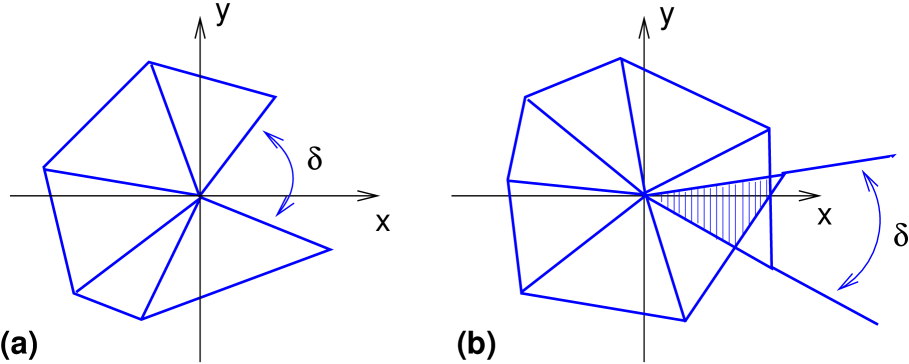
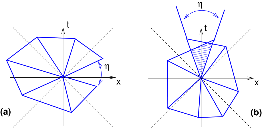
Lorentzian angles are also defined to be additive, in such a way that a complete rotation around a spacelike bone gives in the flat case. However, note that the angles are in general complex, and can become arbitrarily large in the vicinity of the light cone. In their contribution to the action, we have to distinguish between two cases. If the Lorentzian deficit angle is spacelike (Fig. 43a), it contributes as , just like in the Euclidean case. By contrast, if it is timelike (Fig. 43b), the deficit angle contributes with the opposite sign, that is, as . Therefore, both a spacelike defect and a timelike excess increase the action, where as a timelike defect or a spacelike excess decrease it.
The deficit angles in Secs 2.1 and 2.2 were calculated using
| (313) |
for pairs of vectors , and the flat Minkowskian scalar product . By definition, the square roots are positive imaginary for negative arguments.
Appendix 2: Link-reflection positivity in two dimensions
In this appendix we will demonstrate the link-reflection positivity of the discrete model of two-dimensional Lorentzian quantum gravity introduced in [45]. Recall that link reflection is the reflection at a plane of half-integer . We choose it to lie at and fix the boundary spatial lengths at the initial time and the final time to . In order to describe a two-dimensional Lorentzian universe with these boundary conditions, we must not only specify the geometry of the spatial sections (simply given by , ), but the connectivity of the entire two-dimensional triangulation.
A convenient way of parametrizing the connectivity that is symmetric with respect to incoming and outgoing triangles at any given slice of constant is as follows. For any spatial slice at some integer time , each of the spatial edges forms the base of one incoming and one outgoing triangle. The geometry of the adjoining sandwiches is determined by how these triangles are glued together pairwise along their timelike edges. These gluing patterns correspond to distinct ordered partitions of the triangles (either above or below ) into groups, . We denote the partitions collectively by for the incoming triangles and by for the outgoing triangles. The constraints on these variables are obviously and a matching condition for adjacent slices, namely, .343434 This parametrization is closely related to the description of two-dimensional Lorentzian gravity in terms of “half-edges” [43]. In terms of these variables, the (unmarked) one-step propagator is given by
| (314) | |||||
where depends on the two-dimensional cosmological constant . It is obvious from (314) that the propagator depends symmetrically on the local variables and . The partition function for the entire system is
| (315) |
in accordance with (3).
Following the discussion of link reflection in Sec. 6, we consider now functions that depend only on the geometry above the reflecting plane at , i.e. on , , . The reflection (86) acts on the partition data according to and . Without loss of generality, we can assume that depends symmetrically on and , . Computing the expectation value (88), we obtain
i.e.
| (316) | |||||
Since the last expression is a sum of positive terms, we have hereby shown that two-dimensional Lorentzian gravity is link-reflection positive.
References
- [1] S. Weinberg, Ultraviolet divergences in quantum theories of gravitation, in General relativity: Einstein centenary survey, eds. S.W. Hawking and W. Israel (Cambridge University Press, Cambridge, UK, 1979) 790-831.
-
[2]
S. Catterall,
Supersymmetric lattices
[arXiv:1005.5346, hep-lat].
S. Catterall, D.B. Kaplan and M. Unsal, Exact lattice supersymmetry, Phys. Rept. 484 (2009) 71 [arXiv:0903.4881, hep-lat]. -
[3]
H. Kawai and M. Ninomiya,
Renormalization group and quantum gravity,
Nucl. Phys. B 336 (1990) 115.
H. Kawai, Y. Kitazawa and M. Ninomiya, Scaling exponents in quantum gravity near two-dimensions, Nucl. Phys. B 393 (1993) 280-300 [hep-th/9206081].
Ultraviolet stable fixed point and scaling relations in (2+epsilon)-dimensional quantum gravity, Nucl. Phys. B 404 (1993) 684-716 [hep-th/9303123];
Renormalizability of quantum gravity near two dimensions, Nucl. Phys. B 467 (1996) 313-331 [hep-th/9511217].
T. Aida, Y. Kitazawa, H. Kawai and M. Ninomiya, Conformal invariance and renormalization group in quantum gravity near two-dimensions, Nucl. Phys. B 427 (1994) 158-180 [hep-th/9404171]. -
[4]
M. Reuter,
Nonperturbative evolution equation for quantum gravity,
Phys. Rev. D 57 (1998) 971-985 [hep-th/9605030]. -
[5]
A. Codello, R. Percacci and C. Rahmede,
Investigating the ultraviolet properties of gravity with a Wilsonian
renormalization group equation,
Annals Phys. 324 (2009) 414 [arXiv:0805.2909, hep-th].
M. Reuter and F. Saueressig, Functional renormalization group equations, asymptotic safety, and Quantum Einstein Gravity [arXiv:0708.1317, hep-th].
M. Niedermaier and M. Reuter, The asymptotic safety scenario in quantum gravity, Living Rev. Rel. 9 (2006) 5.
H.W. Hamber and R.M. Williams, Nonlocal effective gravitational field equations and the running of Newton’s G, Phys. Rev. D 72 (2005) 044026 [hep-th/0507017].
D.F. Litim, Fixed points of quantum gravity, Phys. Rev. Lett. 92 (2004) 201301 [hep-th/0312114]. -
[6]
A.M. Polyakov,
Compact gauge fields and the infrared catastrophe,
Phys. Lett. B 59 (1975) 82-84;
Quark confinement and topology of gauge groups, Nucl. Phys. B 120 (1977) 429-458. -
[7]
J. Ambjørn, B. Durhuus and J. Fröhlich,
Diseases of triangulated random surface models, and possible cures,
Nucl. Phys. B 257 (1985) 433-449.
J. Ambjørn, B. Durhuus, J. Fröhlich and P. Orland, The appearance of critical dimensions in regulated string theories, Nucl. Phys. B 270 (1986) 457-482. -
[8]
F. David,
Planar diagrams, two-dimensional lattice gravity and surface models,
Nucl. Phys. B 257 (1985) 45.
A. Billoire and F. David, Microcanonical simulations of randomly triangulated planar random surfaces, Phys. Lett. B 168 (1986) 279-283. -
[9]
V.A. Kazakov, A.A. Migdal and I.K. Kostov,
Critical properties of randomly triangulated planar random surfaces,
Phys. Lett. B 157 (1985) 295-300.
D.V. Boulatov, V.A. Kazakov, I.K. Kostov and A.A. Migdal, Analytical and numerical study of the model of dynamically triangulated random surfaces, Nucl. Phys. B 275 (1986) 641-686. -
[10]
J. Ambjørn and S. Varsted,
Three-dimensional simplicial quantum gravity,
Nucl. Phys. B 373 (1992) 557-580;
Entropy estimate in three-dimensional simplicial quantum gravity, Phys. Lett. B 266 (1991) 285-290.
J. Ambjørn, D.V. Boulatov, A. Krzywicki and S. Varsted, The vacuum in three-dimensional simplicial quantum gravity, Phys. Lett. B 276 (1992) 432-436. - [11] M.E. Agishtein and A.A. Migdal, Three-dimensional quantum gravity as dynamical triangulation, Mod. Phys. Lett. A 6 (1991) 1863-1884.
- [12] D.V. Boulatov and A. Krzywicki, On the phase diagram of three-dimensional simplicial quantum gravity, Mod. Phys. Lett. A 6 (1991) 3005-3014.
- [13] J. Ambjørn and J. Jurkiewicz, Four-dimensional simplicial quantum gravity, Phys. Lett. B 278 (1992) 42-50.
- [14] M.E. Agishtein and A.A. Migdal, Simulations of four-dimensional simplicial quantum gravity, Mod. Phys. Lett. A 7 (1992) 1039-1062.
-
[15]
J. Ambjørn and K.N. Anagnostopoulos,
Quantum geometry of 2D gravity coupled to unitary matter,
Nucl. Phys. B 497 (1997) 445 [hep-lat/9701006].
J. Ambjørn, K.N. Anagnostopoulos, U. Magnea and G. Thorleifsson, Geometrical interpretation of the KPZ exponents, Phys. Lett. B 388 (1996) 713 [hep-lat/9606012]. -
[16]
J. Ambjørn, J. Jurkiewicz and Y. Watabiki,
On the fractal structure of two-dimensional quantum gravity,
Nucl. Phys. B 454 (1995) 313 [hep-lat/9507014].
J. Ambjørn and Y. Watabiki, Scaling in quantum gravity, Nucl. Phys. B 445 (1995) 129 [hep-th/9501049]. - [17] S. Catterall, G. Thorleifsson, M.J. Bowick and V. John, Scaling and the fractal geometry of two-dimensional quantum gravity, Phys. Lett. B 354 (1995) 58-68 [hep-lat/9504009].
- [18] J. Ambjørn and J. Jurkiewicz, Scaling in four-dimensional quantum gravity, Nucl. Phys. B 451 (1995) 643-676 [arXiv:hep-th/9503006].
-
[19]
B.V. de Bakker and J. Smit,
Curvature and scaling in 4-d dynamical triangulation,
Nucl. Phys. B 439 (1995) 239-258
[hep-lat/9407014].
S. Catterall, J. B. Kogut and R. Renken, Phase structure of four-dimensional simplicial quantum gravity, Phys. Lett. B 328 (1994) 277-283 [hep-lat/9401026].
H.S. Egawa, T. Hotta, T. Izubuchi, N. Tsuda and T. Yukawa, Scaling behavior in 4-D simplicial quantum gravity, Prog. Theor. Phys. 97 (1997) 539-552 [hep-lat/9611028]. -
[20]
K. Osterwalder and R. Schrader,
Axioms for Euclidean Green’s functions I& II,
Commun. Math. Phys. 31 (1973) 83-112,
42 (1975) 281-305.
E. Seiler, Gauge theories as a problem of constructive quantum field theory and statistical mechanics, Lecture Notes in Physics 159 (Springer, Berlin, 1982).
J. Glimm and A. Jaffe, Quantum physics, second edition (Springer, New York, 1987). - [21] K.S. Stelle, Renormalization of higher derivative quantum gravity, Phys. Rev. D 16 (1977) 953-969.
- [22] J.B. Hartle and S.W. Hawking, Wave function of the universe, Phys. Rev. D 28 (1983) 2960-2975.
- [23] P.O. Mazur and E. Mottola, The path integral measure, conformal factor problem and stability of the ground state of quantum gravity, Nucl. Phys. B 341 (1990) 187-212.
-
[24]
P.D. Mannheim,
Making the case for conformal gravity
[arXiv:1101.2186, hep-th];
Solution to the ghost problem in fourth order derivative theories, Found. Phys. 37 (2007) 532 [hep-th/0608154];
Conformal gravity challenges string theory [arXiv:0707.2283, hep-th]. -
[25]
D. Blas, M. Shaposhnikov and D. Zenhausern,
Scale-invariant alternatives to general relativity,
Phys. Rev. D 84 (2011) 044001
[arXiv:1104.1392, hep-th].
M. Shaposhnikov and D. Zenhausern, Scale invariance, unimodular gravity and dark energy, Phys. Lett. B 671 (2009) 187 [arXiv:0809.3395, hep-th]. -
[26]
P. Hořava,
Quantum gravity at a Lifshitz point,
Phys. Rev. D 79 (2009) 084008
[arXiv:0901.3775, hep-th].
P. Hořava and C.M. Melby-Thompson, General covariance in quantum gravity at a Lifshitz point, Phys. Rev. D 82 (2010) 064027 [arXiv:1007.2410, hep-th];
Anisotropic conformal infinity [arXiv:0909.3841, hep-th]. - [27] A. Ashtekar, D. Marolf, J. Mourao and T. Thiemann, Constructing Hamiltonian quantum theories from path integrals in a diffeomorphism-invariant context, Class. Quant. Grav. 17 (2000) 4919-4940 [quant-ph/9904094].
-
[28]
R. Loll,
Discrete Lorentzian quantum gravity,
Nucl. Phys. Proc. Suppl. 94 (2001) 96
[hep-th/0011194];
A discrete history of the Lorentzian path integral, Lect. Notes Phys. 631 (2003) 137 [hep-th/0212340].
J. Ambjørn, J. Jurkiewicz and R. Loll, Quantum gravity, or The art of building spacetime, in Approaches to quantum gravity, ed. D. Oriti (Cambridge University Press, Cambridge, UK, 2009) 341-359 [hep-th/0604212].
R. Loll, The emergence of spacetime or quantum gravity on your desktop, Class. Quant. Grav. 25 (2008) 114006 [arXiv:0711.0273, gr-qc].
J. Ambjørn, A. Görlich, J. Jurkiewicz and R. Loll, The emergence of (Euclidean) de Sitter space-time, in Path integrals - New trends and perspectives, eds. W. Janke and A. Pelster (World Scientific, Singapore, 2008) 191-198;
The quantum universe, Acta Phys. Polon. B 39 (2008) 3309.
J. Ambjørn, J. Jurkiewicz and R. Loll, Deriving spacetime from first principles, Annalen Phys. 19 (2010) 186;
Causal dynamical triangulations and the quest for quantum gravity, in Foundations of space and time, eds. G. Ellis, J. Murugan and A. Weltman (Cambridge University Press, Cambridge, UK, 2012) [arXiv:1004.0352, hep-th];
Lattice quantum gravity - an update, PoS LATTICE 2010 (2010) 014 [arXiv:1105.5582, hep-lat]. -
[29]
J. Ambjørn, J. Jurkiewicz and R. Loll,
Lorentzian and Euclidean quantum gravity: Analytical and numerical results,
in Proceedings of M-theory and quantum geometry, 1999 NATO
Advanced Study Institute, Akureyri, Island, eds. L. Thorlacius et al.
(Kluwer, 2000) 382-449 [hep-th/0001124];
Quantum gravity as sum over spacetimes, Lect. Notes Phys. 807 (2010) 59 [arXiv:0906.3947, gr-qc].
J. Ambjørn, A. Görlich, J. Jurkiewicz and R. Loll, CDT - an entropic theory of quantum gravity [arXiv:1007.2560, hep-th]. -
[30]
J. Ambjørn, J. Jurkiewicz and R. Loll,
The Universe from scratch,
Contemp. Phys. 47 (2006) 103
[hep-th/0509010];
The self-organized de Sitter universe, Int. J. Mod. Phys. D 17 (2009) 2515 [arXiv:0806.0397, gr-qc];
The self-organizing quantum universe, Sci. Am. 299N1 (2008) 42. - [31] R. Loll, Discrete approaches to quantum gravity in four-dimensions, Living Rev. Rel. 1 (1998) 13 [gr-qc/9805049].
-
[32]
C. Teitelboim,
Causality versus gauge invariance in quantum gravity and supergravity,
Phys. Rev. Lett. 50 (1983) 705-708;
The proper time gauge in quantum theory of gravitation, Phys. Rev. D 28 (1983) 297-309. -
[33]
S. Catterall and E. Mottola,
The conformal mode in 2-D simplicial gravity,
Phys. Lett. B 467 (1999) 29
[hep-lat/9906032];
Reconstructing the conformal mode in simplicial gravity, Nucl. Phys. Proc. Suppl. 83 (2000) 748 [hep-lat/9909074].
S. Catterall, E. Mottola and T. Bhattacharya, Dynamics of the conformal mode and simplicial gravity, Nucl. Phys. Proc. Suppl. 73 (1999) 792 [hep-lat/9809114]. - [34] J. Zinn-Justin, Quantum field theory and critical phenomena, Int. Ser. Monogr. Phys. 113 (2002) 1.
- [35] J. Ambjørn, J. Jurkiewicz and R. Loll, Dynamically triangulating Lorentzian quantum gravity, Nucl. Phys. B 610 (2001) 347-382 [hep-th/0105267].
- [36] T. Regge, General relativity without coordinates, Nuovo Cim. 19 (1961) 558.
-
[37]
J.A. Wheeler,
Geometrodynamics and the issue of the
final state, in Relativity, groups and topology, eds.
B. DeWitt and C. DeWitt (Gordon and Breach, New York, 1964).
J.B. Hartle, Simplicial minisuperspace I. General discussion, J. Math. Phys. 26 (1985) 804-814. - [38] J. Louko and R.D. Sorkin, Complex actions in two-dimensional topology change, Class. Quant. Grav. 14 (1997) 179 [gr-qc/9511023].
- [39] J. Ambjørn, B. Durhuus and T. Jonsson, Quantum geometry. A statistical field theory approach Cambridge University Press, Cambridge, UK, 1997)
- [40] J. Ambjørn, M. Carfora and A. Marzuoli, The geometry of dynamical triangulations, Lecture Notes in Physics, New Series, m 50 (Springer, Berlin, 1997) [hep-th/9612069].
-
[41]
J. Ambjørn and J. Jurkiewicz,
On the exponential bound in four-dimensional simplicial gravity,
Phys. Lett. B 335 (1994) 355-358
[hep-lat/9405010].
B. Brügmann and E. Marinari, More on the exponential bound of four-dimensional simplicial quantum gravity, Phys. Lett. B 349 (1995) 35-41 [hep-th/9411060]. - [42] R. Nakayama, 2-D quantum gravity in the proper time gauge, Phys. Lett. B 325 (1994) 347 [hep-th/9312158].
- [43] P. Di Francesco, E. Guitter and C. Kristjansen, Integrable 2d Lorentzian gravity and random walks, Nucl. Phys. B 567 (2000) 515-553 [hep-th/9907084].
- [44] I. Montvay and G. Münster, Quantum fields on a lattice (Cambridge University Press, Cambridge, UK, 1994).
- [45] J. Ambjørn and R. Loll, Non-perturbative Lorentzian quantum gravity, causality and topology change, Nucl. Phys. B 536 (1998) 407-434 [hep-th/9805108].
- [46] J. Ambjørn, R. Loll, J.L. Nielsen and J. Rolf, Euclidean and Lorentzian quantum gravity: Lessons from two-dimensions, Chaos Solitons Fractals 10 (1999) 177-195 [hep-th/9806241].
- [47] S. Zohren, A causal perspective on random geometry [arXiv:0905.0213, hep-th].
- [48] P. Di Francesco, E. Guitter and C. Kristjansen, Generalized Lorentzian gravity in (1+1)D and the Calogero Hamiltonian, Nucl. Phys. B 608 (2001) 485-526 [hep-th/0010259].
- [49] M. Ansari and F. Markopoulou, A statistical formalism of causal dynamical triangulations, Nucl. Phys. B 726 (2005) 494-509 [hep-th/0505165].
- [50] B. Durhuus and C.W.H. Lee, A string bit Hamiltonian approach to two-dimensional quantum gravity, Nucl. Phys. B 623 (2002) 201 [hep-th/0108149].
- [51] F. Markopoulou and L. Smolin, Gauge fixing in causal dynamical triangulations, Nucl. Phys. B 739 120-130 [hep-th/0409057].
- [52] J. Ambjørn, K.N. Anagnostopoulos and R. Loll: A new perspective on matter coupling in 2d quantum gravity, Phys. Rev. D 60 (1999) 104035 [hep-th/9904012].
- [53] J. Ambjørn, K.N. Anagnostopoulos, R. Loll and I. Pushkina, Shaken, but not stirred - Potts model coupled to quantum gravity, Nucl. Phys. B 807 (2009) 251 [arXiv:0806.3506, hep-lat].
-
[54]
D. Benedetti and R. Loll,
Unexpected spin-off from quantum gravity,
Physica A 377 (2007) 373
[hep-lat/0603013];
Quantum gravity and matter: Counting graphs on causal dynamical triangulations, Gen. Rel. Grav. 39 (2007) 863 [gr-qc/0611075]. - [55] J. Ambjørn, R. Loll, W. Westra and S. Zohren, Putting a cap on causality violations in CDT, JHEP 0712 (2007) 017 [arXiv:0709.2784, gr-qc].
- [56] J. Ambjørn, R. Loll, Y. Watabiki, W. Westra and S. Zohren, A string field theory based on causal dynamical triangulations, JHEP 0805 (2008) 032 [arXiv:0802.0719, hep-th].
-
[57]
J. Ambjørn, R. Loll, W. Westra and S. Zohren,
A matrix model for 2D quantum gravity defined by causal dynamical
triangulations,
Phys. Lett. B 665 (2008) 252-256 [arXiv:0804.0252, hep-th];
A new continuum limit of matrix models, Phys. Lett. B 670 (2008) 224 [arXiv:0810.2408, hep-th].
D. Benedetti and J. Henson, Imposing causality on a matrix model, Phys. Lett. B 678 (2009) 222-226 [arXiv:0812.426, hep-th]. - [58] J. Ambjørn, R. Janik, W. Westra and S. Zohren, The emergence of background geometry from quantum fluctuations, Phys. Lett. B 641 (2006) 94 [gr-qc/0607013].
- [59] M. Ikehara, N. Ishibashi, H. Kawai, T. Mogami, R. Nakayama and N. Sasakura, A note on string field theory in the temporal gauge, Prog. Theor. Phys. Suppl. 118 (1995) 241-258 [hep-th/9409101].
- [60] J. Ambjørn, R. Loll, W. Westra and S. Zohren, Stochastic quantization and the role of time in quantum gravity, Phys. Lett. B 680 (2009) 359-364 [arXiv:0908.4224, hep-th].
- [61] F. David, Loop equations and nonperturbative effects in two-dimensional quantum gravity, Mod. Phys. Lett. A 5 (1990) 1019-1030.
-
[62]
J. Ambjørn, J. Jurkiewicz and Y.M. Makeenko,
Multiloop correlators for two-dimensional quantum gravity,
Phys. Lett. B 251 (1990) 517-524.
J. Ambjørn, C.F. Kristjansen, Y.M. Makeenko, Higher genus correlators for the complex matrix model, Mod. Phys. Lett. A 7 (1992) 3187-3202 [hep-th/9207020].
J. Ambjørn, L. Chekhov, C.F. Kristjansen and Y.M. Makeenko, Matrix model calculations beyond the spherical limit, Nucl. Phys. B 404 (1993) 127-172 [hep-th/9302014]. - [63] J. Ambjørn, R. Loll, W. Westra and S. Zohren, Summing over all topologies in CDT string field theory, Phys. Lett. B 678 (2009) 227-232 [arXiv:0905.2108, hep-th].
- [64] J. Ambjørn, J. Correia, C. Kristjansen and R. Loll, On the relation between Euclidean and Lorentzian 2-D quantum gravity, Phys. Lett. B 475 (2000) 24-32 [hep-th/9912267].
- [65] D.V. Boulatov and V.A. Kazakov, The Ising model on random planar lattice: The structure of phase transition and the exact critical exponents, Phys. Lett. B 186 (1987) 379.
-
[66]
V.G. Knizhnik, A.M. Polyakov and A.B. Zamolodchikov,
Fractal structure of 2D quantum gravity,
Mod. Phys. Lett. A 3 (1988) 819.
F. David, Conformal field theories coupled to 2D gravity in the conformal gauge, Mod. Phys. Lett. A 3 (1988) 1651.
J. Distler and H. Kawai, Conformal field theory and 2D quantum gravity or Who’s afraid of Joseph Liouville?, Nucl. Phys. B 321 (1989) 509. -
[67]
J. Ambjørn, B. Durhuus and T. Jonsson,
A Solvable 2-d gravity model with gamma 0,
Mod. Phys. Lett. A 9 (1994) 1221
[hep-th/9401137].
J. Ambjørn, B. Durhuus, T. Jonsson and G. Thorleifsson, Matter fields with c 1 coupled to 2-d gravity, Nucl. Phys. B 398 (1993) 568 [hep-th/9208030]. -
[68]
J. Ambjørn, J. Jurkiewicz, R. Loll and G. Vernizzi,
Lorentzian 3d gravity with wormholes via matrix models,
JHEP 0109 (2001) 022 [hep-th/0106082];
3D Lorentzian quantum gravity from the asymmetric ABAB matrix model, Acta Phys. Polon. B 34 (2003) 4667-4688 [hep-th/0311072].
J. Ambjørn, J. Jurkiewicz and R. Loll, Renormalization of 3d quantum gravity from matrix models, Phys. Lett. B 581 (2004) 255-262 [hep-th/0307263]. - [69] B. Dittrich and R. Loll, A hexagon model for 3-D Lorentzian quantum cosmology, Phys. Rev. D 66 (2002) 084016 [hep-th/0204210].
- [70] D. Benedetti, R. Loll and F. Zamponi, (2+1)-dimensional quantum gravity as the continuum limit of causal dynamical triangulations, Phys. Rev. D 76 (2007) 104022 [arXiv:0704.3214, hep-th].
- [71] J. Ambjørn, J. Jurkiewicz and R. Loll, Non-perturbative 3d Lorentzian quantum gravity, Phys. Rev. D 64 (2001) 044011 [hep-th/0011276].
- [72] J. Henson, Coarse graining dynamical triangulations: A new scheme, Class. Quant. Grav. 26 (2009) 175019 [arXiv:0907.5602, gr-qc].
-
[73]
U. Pachner,
Bistellare Äquivalenz kombinatorischer
Mannigfaltigkeitten, Arh.Math. 30 (1978) 89.
M. Gross and S. Varsted, Elementary moves and ergodicity in D-dimensional simplicial quantum gravity, Nucl. Phys. B 378 (1992) 367-380. - [74] B. Dittrich and R. Loll, Counting a black hole in Lorentzian product triangulations, Class. Quant. Grav. 23 (2006) 3849-3878
-
[75]
S. Catterall, J.B. Kogut and R. Renken,
Is there an exponential bound in four-dimensional simplicial gravity?,
Phys. Rev. Lett. 72 (1994) 4062-4065
[hep-lat/9403019].
B.V. De Bakker and J. Smit, Volume dependence of the phase boundary in 4-D dynamical triangulation, Phys. Lett. B 334 (1994) 304-308 [hep-lat/9405013]. -
[76]
J. Ambjørn, J. Jurkiewicz and R. Loll,
A non-perturbative Lorentzian path integral for gravity,
Phys. Rev. Lett. 85 (2000) 924 [hep-th/0002050];
Dynamically triangulating Lorentzian quantum gravity, Nucl. Phys. B 610 (2001) 347-382 [hep-th/0105267]. - [77] J. Ambjørn, J. Jurkiewicz and R. Loll, Emergence of a 4D world from causal quantum gravity, Phys. Rev. Lett. 93 (2004) 131301 [hep-th/0404156].
- [78] J. Ambjørn, J. Jurkiewicz and R. Loll, Reconstructing the universe, Phys. Rev. D 72 (2005) 064014 [hep-th/0505154].
-
[79]
J. Ambjørn, S. Jain, J. Jurkiewicz and C.F. Kristjansen,
Observing 4-d baby universes in quantum gravity,
Phys. Lett. B 305 (1993) 208-213
[hep-th/9303041].
J. Ambjørn, S. Jain and G. Thorleifsson, Baby universes in 2-d quantum gravity, Phys. Lett. B 307 (1993) 34-39 [hep-th/9303149]. - [80] J. Ambjørn, P. Bialas, J. Jurkiewicz, Z. Burda and B. Petersson, Effective sampling of random surfaces by baby universe surgery, Phys. Lett. B 325 (1994) 337-346 [hep-lat/9401022].
- [81] J. Ambjørn, A. Görlich, S. Jordan, J. Jurkiewicz and R. Loll, CDT meets Hořava-Lifshitz gravity, Phys. Lett. B 690 (2010) 413-419 [arXiv:1002.3298, hep-th].
- [82] J. Ambjørn, S. Jordan, J. Jurkiewicz and R. Loll, A second-order phase transition in CDT, Phys. Rev. Lett. 107 (2011) 211303 [arXiv:1108.3932, hep-th].
- [83] J. Ambjørn, A. Görlich, J. Jurkiewicz and R. Loll, Planckian birth of the quantum de Sitter universe, Phys. Rev. Lett. 100 (2008) 091304 [arXiv:0712.2485, hep-th].
- [84] J. Ambjørn, A. Görlich, J. Jurkiewicz and R. Loll, The nonperturbative quantum de Sitter universe, Phys. Rev. D 78 (2008) 063544 [arXiv:0807.4481, hep-th].
- [85] J. Ambjørn, J. Jurkiewicz and R. Loll, Semiclassical universe from first principles, Phys. Lett. B 607 (2005) 205-213 [hep-th/0411152].
- [86] J. Ambjørn, A. Görlich, J. Jurkiewicz and R. Loll, Geometry of the quantum universe, Phys. Lett. B 690 (2010) 420-426 [arXiv:1001.4581, hep-th].
- [87] R.M. Hornreich, M. Luban and S. Shtrikman, Critical behavior at the onset of -space instability on the line, Phys. Rev. Lett. 35 (1975) 1678.
- [88] N. Goldenfeld, Lectures on phase transitions and the renormalization group, Addison-Wesley, Reading (Mass.) (1992).
-
[89]
S. Catterall, G. Thorleifsson, J.B. Kogut and R. Renken,
Singular vertices and the triangulation space of the D sphere,
Nucl. Phys. B 468 (1996) 263-276
[hep-lat/9512012].
P. Bialas, Z. Burda, B. Petersson and J. Tabaczek, Appearance of mother universe and singular vertices in random geometries, Nucl. Phys. B 495 (1997) 463-476 [hep-lat/9608030]. -
[90]
P. Bialas, Z. Burda, A. Krzywicki and B. Petersson,
Focusing on the fixed point of 4-D simplicial gravity,
Nucl. Phys. B 472 (1996) 293-308
[hep-lat/9601024].
S. Catterall, R. Renken and J.B. Kogut, Singular structure in 4-D simplicial gravity, Phys. Lett. B 416 (1998) 274-280 [hep-lat/9709007]. - [91] J. Ambjørn and B. Durhuus, Regularized bosonic strings need extrinsic curvature, Phys. Lett. B 188 (1987) 253.
- [92] B. Durhuus, J. Fröhlich and T. Jonsson, Critical behavior in a model of planar random surfaces, Nucl. Phys. B 240 (1984) 453; Phys. Lett. B 137 (1984) 93.
- [93] F. David, A scenario for the c 1 barrier in noncritical bosonic strings, Nucl. Phys. B 487 (1997) 633-649 [hep-th/9610037].
- [94] J. Ambjørn, A. Dasgupta, J. Jurkiewicz and R. Loll, A Lorentzian cure for Euclidean troubles, Nucl. Phys. Proc. Suppl. 106 (2002) 977 [hep-th/0201104].
- [95] A. Dasgupta and R. Loll, A proper time cure for the conformal sickness in quantum gravity, Nucl. Phys. B 606 (2001) 357 [hep-th/0103186].
- [96] J. Ambjørn, A. Görlich, J. Jurkiewicz, R. Loll, J. Gizbert-Studnicki and T. Trzesniewski, The semiclassical limit of causal dynamical triangulations, Nucl. Phys. B 849 (2011) 144 [arXiv:1102.3929, hep-th].
- [97] O. Lauscher and M. Reuter, Fractal spacetime structure in asymptotically safe gravity, JHEP 0510 (2005) 050 [hep-th/0508202].
-
[98]
T. Budd,
The effective kinetic term in CDT
[arXiv:1110.5158, gr-qc].
T. Budd and R. Loll, to appear. - [99] E. Kiritsis and G. Kofinas, Hořava-Lifshitz cosmology, Nucl. Phys. B 821 (2009) 467 [arXiv:0904.1334, hep-th].
- [100] R. Brandenberger, Matter bounce in Hořava-Lifshitz cosmology, Phys. Rev. D 80 (2009) 043516 [arXiv:0904.2835, hep-th].
- [101] G. Calcagni, Cosmology of the Lifshitz universe, JHEP 0909 (2009) 112 [arXiv:0904.0829, hep-th].
- [102] D. Benedetti and J. Henson, Spectral geometry as a probe of quantum spacetime, Phys. Rev. D 80 (2009) 124036 [arXiv:0911.0401, hep-th].
- [103] T. Jonsson and J.F. Wheater, The spectral dimension of the branched polymer phase of two-dimensional quantum gravity, Nucl. Phys. B 515 (1998) 549-574 [hep-lat/9710024].
- [104] J. Ambjørn, D. Boulatov, J.L. Nielsen, J. Rolf and Y. Watabiki, The spectral dimension of 2D quantum gravity, JHEP 9802 (1998) 010 [hep-th/9801099].
- [105] J. Ambjørn, K.N. Anagnostopoulos, T. Ichihara, L. Jensen and Y. Watabiki, Quantum geometry and diffusion, JHEP 9811 (1998) 022 [hep-lat/9808027].
- [106] J. Ambjørn and K.N. Anagnostopoulos, Quantum geometry of 2D gravity coupled to unitary matter, Nucl. Phys. B 497 (1997) 445-478 [hep-lat/9701006].
- [107] J. Ambjørn, J. Jurkiewicz and Y. Watabiki, On the fractal structure of two-dimensional quantum gravity, Nucl. Phys. B 454 (1995) 313-342 [hep-lat/9507014].
- [108] J. Ambjørn, J. Jurkiewicz and R. Loll, Spectral dimension of the universe, Phys. Rev. Lett. 95 (2005) 171301 [hep-th/0505113].
- [109] J. Ambjørn, K.N. Anagnostopoulos, T. Ichihara, L. Jensen, N. Kawamoto, Y. Watabiki and K. Yotsuji, Quantum geometry of topological gravity, Phys. Lett. B 397 (1997) 177-184 [hep-lat/9611032].
- [110] M.R. Atkin, G. Giasemidis and J.F. Wheater, Continuum random combs and scale dependent spectral dimension [arXiv:1101.4174, hep-th].
- [111] P. Hořava, Spectral dimension of the universe in quantum gravity at a Lifshitz point, Phys. Rev. Lett. 102 (2009) 161301 [arXiv:0902.3657, hep-th].
-
[112]
S. Carlip,
Spontaneous dimensional reduction in short-distance quantum gravity?
[arXiv:0909.3329, gr-qc];
The small scale structure of spacetime [arXiv:1009.1136, gr-qc].
S. Carlip, R.A. Mosna and J.P.M. Pitelli, Vacuum fluctuations and the small scale structure of spacetime [arXiv:1103.5993, gr-qc]. -
[113]
T.P. Sotiriou, M. Visser and S. Weinfurtner,
Spectral dimension as a probe of the ultraviolet continuum regime of causal dynamical triangulations,
Phys. Rev. Lett. 107 (2011) 131303
[arXiv:1105.5646, gr-qc];
From dispersion relations to spectral dimension - and back again, Phys. Rev. D 84 (2011) 104018 [arXiv:1105.6098, hep-th].
M. Reuter and F. Saueressig, Fractal space-times under the microscope: A renormalization group view on Monte Carlo data, JHEP 1112 (2011) 012 [arXiv:1110.5224, hep-th]. - [114] S. Bilke, Z. Burda, A. Krzywicki, B. Petersson, J. Tabaczek and G. Thorleifsson, 4-D simplicial quantum gravity interacting with gauge matter fields, Phys. Lett. B 418 (1998) 266 [hep-lat/9710077].
- [115] S. Bilke, Z. Burda, A. Krzywicki, B. Petersson, J. Tabaczek and G. Thorleifsson, 4-D simplicial quantum gravity: Matter fields and the corresponding effective action, Phys. Lett. B 432 (1998) 279 [hep-lat/9804011].
- [116] J. Ambjørn, K.N. Anagnostopoulos and J. Jurkiewicz, Abelian gauge fields coupled to simplicial quantum gravity, JHEP 9908 (1999) 016 [hep-lat/9907027].
- [117] J. Laiho and D. Coumbe, Evidence for asymptotic safety from lattice quantum gravity, Phys. Rev. Lett. 107 (2011) 161301 [arXiv:1104.5505, hep-lat].
- [118] C. Anderson, S.J. Carlip, J.H. Cooperman, P. Hořava, R.K. Kommu and P.R. Zulkowski, Quantizing Horava-Lifshitz gravity via causal dynamical triangulations, Phys. Rev. D 85 (2012) 044027, 049904(E) [arXiv:1111.6634, hep-th].
- [119] R.L. Maitra, Can causal dynamical triangulations probe factor-ordering issues?,, Acta Phys. Polon. Supp. 2 (2009) 563 [arXiv:0910.2117, gr-qc].
-
[120]
J. Ambjørn, Z. Burda, J. Jurkiewicz and C.F. Kristjansen,
4-d quantum gravity coupled to matter,
Phys. Rev. D 48 (1993) 3695-3703 [hep-th/9303042].
R.L. Renken, S.M. Catterall and J.B. Kogut, Three-dimensional quantum gravity coupled to Ising matter, Nucl. Phys. B 389 (1993) 601-610 [hep-lat/9205029].
J. Ambjørn, J. Jurkiewicz, S. Bilke, Z. Burda and B. Petersson, Z(2) gauge matter coupled to 4-D simplicial quantum gravity, Mod. Phys. Lett. A 9 (1994) 2527-2542. - [121] J. Ambjørn, K.N. Anagnostopoulos and J. Jurkiewicz, Abelian gauge fields coupled to simplicial quantum gravity, JHEP 9908 (1999) 016 [hep-lat/9907027].
- [122] S. Horata, H.S. Egawa, N. Tsuda and T. Yukawa, Phase structure of four-dimensional simplicial quantum gravity with a U(1) gauge field, Prog. Theor. Phys. 106 (2001) 1037-1050 [hep-lat/0004021].
-
[123]
B.V. de Bakker and J. Smit,
Gravitational binding in 4D dynamical triangulation,
Nucl. Phys. B 484 (1997) 476-494 [hep-lat/9604023];
Correlations and binding in 4-D dynamical triangulation, Nucl. Phys. Proc. Suppl. 47 (1996) 613-616. [hep-lat/9510041];
Euclidean gravity attracts, Nucl. Phys. Proc. Suppl. 34 (1994) 739-741 [hep-lat/9311064]. - [124] I. Khavkine, R. Loll and P. Reska, Coupling a point-like mass to quantum gravity with causal dynamical triangulations Class. Quant. Grav. 27 (2010) 185025 [arXiv:1002.4618, gr-qc].