Correlators of Hopf Wilson loops in the AdS/CFT correspondence
Abstract
We study at quantum level correlators of supersymmetric Wilson loops with contours lying on Hopf fibers of . In SYM theory the strong coupling analysis can be performed using the AdS/CFT correspondence and a connected classical string surface, linking two different fibers, is presented. More precisely, the string solution describes oppositely oriented fibers with the same scalar coupling and depends on an angular parameter, interpolating between a non-BPS configuration and a BPS one. The system can be thought as an alternative deformation of the ordinary antiparallel lines giving the static quark-antiquark potential, that is indeed correctly reproduced, at weak and strong coupling, as the fibers approach one another.
I Introduction
The Wilson loop is one of the most important observable in gauge theories and it has been suspected for a long time that its dynamics should have a natural description in terms of strings. The AdS/CFT correspondence provides a concrete realization of this idea: the quantum expectation value of Wilson loops in Super Yang-Mills theory (SYM4) can be computed by means of the partition function of the type IIB string in , satisfying suitable boundary conditions pot1 ; mwloop ; dgo . Considering as the gauge group and denoting the coupling constant by , the large and strong-coupling limit is equivalent to a semiclassical approximation and the computation reduces to find the minimal area surfaces in , with boundary conditions imposed by the Wilson loop operators.
In addition to the familiar interaction with the gauge field, Wilson loops in SYM4 naturally contain scalar fields coupled to the contour, a presence that can be easily traced back from both sides of the correspondence pot1 ; mwloop ; dgo . It turns out that for suitable choices of the scalar couplings, as functions of the loop variables, the resulting Wilson loop appears to be , i.e. invariant with respect to some of the supersymmetry transformations of the theory. A general class of such operators was proposed by Zarembo Zarembo:2002an and have trivial expectation value. A second family of supersymmetric Wilson loops (that we denote as DGRT), having instead a non-trivial dependence on the gauge coupling constant, was constructed in dgrta , the well studied circular loop eszcircularloop ; drukkergrossexact being a particular representative of this ensemble. The contours lay, in general, into a sphere embedded into the Euclidean and the operators are generically 1/16 BPS. The maximal supersymmetric configuration is the 1/2 BPS circular case, whose exact expectation value is captured by a Gaussian matrix model eszcircularloop ; drukkergrossexact as result of a localization procedure matrixmodelloc . When restricted on the loops are at least 1/8 BPS and a tight relation with two-dimensional Yang-Mills theory on the sphere has been observed dgrta ; Young:2008ed ; Bassetto:2008yf ; Giombi:2009ms ; Bassetto:2009rt ; Bassetto:2009ms ; Giombi:2009ds ; Pestun:2009nn . Recently a systematic classification of supersymmetric Wilson loops invariant under at least one superconformal symmetry has been presented Dymarsky:2009si : weak and strong coupling computations for some new loops appear in Cardinali:2012sy .
Supersymmetric Wilson loops are important objects to study for many reasons. For example, they provide non-trivial tests on the validity of the AdS/CFT correspondence: due to their BPS nature, one can hope to obtain exact results in the gauge theory to be compared with the strong coupling predictions on the string side. For the 1/2 BPS circular loop the exact quantum field theoretical result is indeed reproduced by the classical string computation eszcircularloop ; drukkergrossexact , while the first subleading term was checked in Kruczenski:2008zk . More recently the same limit has been performed, starting from the matrix model obtained by localization in matrixmodelloc , for the BPS circular loop in Superconformal QCD, suggesting a logarithmic behavior of the effective string tension on the ’t Hooft coupling Passerini:2011fe . On the other hand, also non-supersymmetric configurations are of great importance. For instance, as is well known, the non-BPS antiparallel lines allow to define and compute the static quark-antiquark potential pot1 ; mwloop ; pot2 ; Pineda:2007kz and the strong coupling limit can be carefully studied at subleading level Chu:2009qt ; Forini:2010ek . More recently a generalized configuration Drukker:2011za , interpolating between BPS and non-BPS operators, has been introduced and studied both at weak and strong coupling level: in this framework a new non-supersymmetric observable can be defined and exactly computed Correa:2012at ; Correa:2012hh ; Drukker:2012de .
Configurations involving more than one circuit at once (usually two) define Wilson loop correlators. These objects are also very interesting since they carry information about loop interactions: on the string theory side of the correspondence there is the very suggestive picture that a connected correlator is described by a minimal area surface linking the boundary loops grossooguriphase . At QFT level, OPE provides an useful tool to study their operatorial content twotwo ; Arutyunov:2001hs while BPS correlators have been helpful in checking the correspondence among DGRT loops on and two-dimensional Yang-Mills Bassetto:2009rt ; Bassetto:2009ms ; Giombi:2009ds . Due to their more complicated geometry, Wilson loop correlators are much more difficult to face, in gauge theory as well as in string theory. When they can be handled, they reveal a rich phenomenology: for example, the correlator of two parallel and concentric circles exhibits at strong-coupling a sort of phase transition, the so-called Gross-Ooguri phase transition grossooguriphase ; gophase1 ; gophase2 .
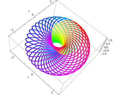
Due to the simple geometry, the most studied correlators involve (anti-)parallel lines and circles inside . An interesting topologically non-trivial configuration involving great circles is provided by the Hopf fibration of : the non-intersecting fibers are in fact “pierced” together in such a way they cannot be separated. The Hopf fibration has been introduced in the context of Wilson loops in dgrta , and it can be naturally considered within the DGRT construction: supersymmetry is also preserved when all the fibers in the same fibration couple the same scalar field with constant coupling. Quite surprisingly the relevant gauge theory propagator between any two points on any two fibers is constant, in Feynman gauge: this suggests that the correlator of any number of Hopf fibers is captured by the same matrix model of the 1/2 BPS circular loop, with different insertion, if interacting diagrams do not contribute. Conversely we would expect that the large , strong-coupling result should be described, at string level, by disconnected world-sheet configurations. While in general there is no reason to believe that interacting diagrams do not contribute, this fact holds true for a single great circle due to its BPS nature: it is natural wondering whether the same simplification occurs also for the BPS configuration involving two Hopf fibers.
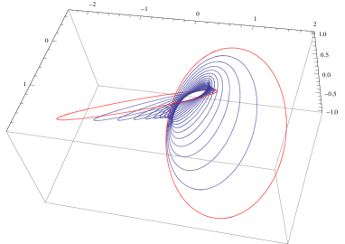
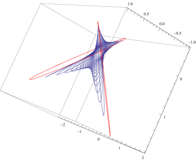
In this paper we have tried to give an answer to this question from the string theory point of view, namely we have studied whether a connected minimal area surface connecting two Hopf fibers is subleading with respect to the disconnected solution, or if it does not exist at all. While we have been able to give only a partial answer to this problem, we have found an interesting connected non-BPS string configuration solving the equations of motion with the appropriate boundary conditions. Geometrically, the found solution describes a connected surface linking the Hopf fibers, and it turns out to have smaller area than the disconnected configuration. Moreover, an interesting dynamics resembling the Gross-Ooguri phase transition appears: the connected solution depends on the fiber angular separation in the Hopf base and when the fibers have maximal angular separation, the connected solution degenerates into the disconnected one. As soon as the separation is smaller, the connected solution is distinct from the disconnected one and it has smaller area than the latter. As we will explain in details, the surface describes antiparallel Hopf fibers with the same scalar coupling and hence gives rise to a non-BPS configuration: we will argue that the BPS configuration involving two antiparallel Hopf fibers (with the correct scalar coupling) does not admit any connected string solution, and presumably the parallel fibers neither.
Interestingly enough, the surface associated to the maximal separation is indeed BPS, hence, by moving the fiber angular separation, our solution is able to continuously interpolate between non-BPS and BPS configurations. Moreover, as we will see, the connected world-sheet provides a string description of a system which can be thought of as a deformation of the ordinary antiparallel lines (in the sense explained in the text), representing a sort of deformation of the usual static quark-antiquark potential. We remark that these same topics have been recently discussed in Drukker:2011za for the case of the circular loop and antiparallel lines.
The paper is organized as follows. In order to fix some notation, we are going to continue this introduction by briefly reviewing how DGRT Wilson loops are defined, the geometry of the Hopf fibration and the AdS/CFT prescription to compute Wilson loop expectation values, tools we will need for our computations. In sec. II we will present the derivation of the minimal area surface in satisfying the desired boundary conditions. In sec. III we will study the properties of the connected solution in the case of constant (no motion in ) and non-constant (motion in ) scalar couplings. In sec. IV we will discuss the supersymmetry of the solutions we found. In sec. V we will explain how the found solution should be interpreted from the gauge theory viewpoint, explaining its relation with the quark-antiquark potential. We will check at perturbative level the consistency of our interpretation. In sec. VI we will summarize the results, making some comments on the open questions and the directions worth to be studied in the future.
I.1 The DGRT Wilson loops
The relevant Wilson loop operator in SYM4 is given by mwloop ; pot1 ; dgo (in Euclidean signature)
| (1) |
where is the gauge connection, are the six scalars of the vector multiplet, are coordinates and are coordinates parameterizing a path in along the loop with parameter .
We would like to consider space-time paths lying on some embedded111 can also be seen as a fixed time slice of the compactification . into . One can construct a generalized gauge connection involving the scalar fields using right-invariant 1-forms: in Euclidean coordinates , constrained by , they are given by 222We follow the conventions of dgrta .
| (2) |
A DGRT Wilson loop is defined by assigning the scalar couplings
| (3) |
where the constant matrix is norm preserving333Because of the symmetry, one can consider ., i.e. it satisfies
| (4) |
We immediately see that444For a discussion about the origin of this constraint see for example dgo . . As shown in dgrta , a DGRT loop is generically 1/16 BPS and supersymmetry is enhanced for particular contours. For example, the familiar 1/2 BPS circular loop, defined by
| (5) |
belongs to this class, the pullback on the loop of the right-invariant 1-forms being
| (6) |
yielding a constant coupling to only. Its exact quantum expectation value is known: in Feynman gauge interacting diagrams do not contribute, while the constancy of the combined gauge-scalar propagator on the loop
| (7) |
allows to sum up all the ladder diagrams, giving the following matrix model representation eszcircularloop ; drukkergrossexact
| (8) |
where is a constant Hermitian matrix. In particular, in the large , limit one has
| (9) |
The same matrix model has been obtained in matrixmodelloc by formulating the theory on and applying a localization procedure to compute exactly the path-integral: actually, in the same paper, a much more general matrix integral has been derived for superconformal theories, including non-trivial instanton corrections.
I.2 The Hopf fibration
From the geometrical point of view can be described as a non-trivial bundle over : the construction is known as the Hopf fibration. Its structure becomes transparent by parameterizing by555We will refer to these angles as Hopf coordinates.
| (10) |
and projecting with the Hopf map
| (11) |
The projection reveals that parameterize the base while the fibers , which are non-intersecting great circles inside .
The Hopf fibration has been introduced in the context of supersymmetric Wilson loops in dgrta . By expressing the right invariant 1-forms in Hopf coordinates
| (12) |
we can see that all the fibers in the same fibration couple to the same scalar. In fact, at constant we have
| (13) |
as in (6). Remarkably the loops share half the supersymmetries of a single circle, the system being effectively 1/4 BPS. The corresponding preserved supercharges will be essentially the same as the ones associated to the 1/2 BPS maximal circle, except that only one chirality is selected dgrta . It is therefore natural to expect that correlators of Hopf fibers should be exactly computable, due to their BPS character. At perturbative level we observe another peculiar feature pointing in this direction, namely that in a configuration made of Hopf fibers, the gauge-scalar propagator (in Feynman gauge) between any pair of points , on any fiber is the same constant as in (7). As pointed out in dgrta , this implies that all the ladder diagrams contributing to the correlator of fibers are summed up by the same matrix model of the 1/2 BPS circle (8), but with a different insertion
| (14) |
As mentioned in the beginning, in the large limit the ladder correlator will be the same as non-interacting circles, and it will be reproduced at strong coupling by disconnected string surfaces. The absence of dominant connected configurations would be a stringy support to the conjecture about the exactness of the matrix model666This conjecture is also supported by the cancellation of the lowest order diagrams containing interactions PCom . for the Hopf fibration dgrta .
I.3 The string description of Wilson loops in SYM
The AdS/CFT prescription to compute the expectation value of Wilson loops, originally proposed in mwloop ; pot1 , can be schematically described as
| (15) |
where is the string action in the background and represents all the string coordinates. The sum over the string world-sheets is taken over those ending on the loop and lying along (at the AdS boundary). These boundary conditions arise in a natural way by considering the 10-dimensional nature of SYM4 (see dgo for a detailed derivation).
The string action is given by a non-linear sigma model777The original derivation of the full action can be found in adsstring . We are interested just in the leading semiclassical approximation of the path-integral, where the fermions can be taken vanishing. We display therefore only the bosonic sector of the full action., namely
| (16) |
where are world-sheet coordinates, is the world-sheet metric and is the metric: the action is classically equivalent to the area functional. Using the equations, that is the vanishing of the world-sheet energy-momentum tensor
| (17) |
the action becomes
| (18) |
where denotes the induced metric on the world-sheet. In the large limit, the expectation value of a Wilson loop at strong coupling is computed as a classical solution of the string equations (i.e. the minimal area surface) in with the boundary conditions imposed by the loop and the scalar couplings
| (19) |
In the next section we are finally going to face the problem of finding a minimal string surface ending on a pair of Hopf fibers. It is worth to outline the strategy:
-
-
We will begin by writing the sigma model employing a coordinate system adapted to the Hopf fibration (10).
-
-
We will give a natural ansatz based on the Hopf fibration and geometries. This allows us to simplify the problem.
-
-
We will verify that the ansatz gives a consistent solution, and we will discuss its properties.
II The string description of Hopf fiber correlators
We will work in the conformal gauge, namely we will consider world-sheet coordinates such that (Euclidean signature). Then the equations must be imposed as constraints (Virasoro constraints)
| (20) |
while the equations describe a geodesic-like motion888We mean that the lines or are geodesics of the target space. in . Thanks to the product geometry of the target space, coordinates where is diagonal with respect to the factor spaces can be chosen, namely
| (21) |
where , are coordinates and metric on , and , are coordinates and metric on . The world-sheet energy-momentum tensor and the induced metric receive separate contributions from the two factors, ending up with two distinct sigma models
| (22) |
which must be solved with the following boundary conditions (schematically)
| (23) |
However, the systems are still interacting through the Virasoro constraints
| (24) |
and through the world-sheet coordinates, which must be the same on both the factor spaces.
II.1 motion
We will work with in global coordinates
| (25) |
where the metric takes the form
| (26) |
In this coordinate system the AdS boundary is mapped to . Moreover, since the 3-sphere at infinity parametrized by is naturally identified with a fixed time slice of the global AdS boundary , we will employ a coordinate system adapted to the Hopf fibration (10)
| (27) |
The metric reads as
| (28) |
so that the metric with respect to is given by
| (29) |
We will take the world-sheet coordinates to be ; differentiation with respect to and will be denoted by a dot and a prime respectively. The form of the metric suggests the following notation
| (30) |
representing the metric tensor 999 transforms as a tensor with respect to coordinate changes of the form In particular, it is a tensor with respect to reparameterizations of . of . By setting , the induced metric is explicitly given by
| (31) |
II.2 motion
We begin by considering the 5-sphere parametrized by , . As far as DGRT loops are concerned, we can limit to consider a non-trivial motion in a subspace dgrta . By setting and parameterizing the relevant sphere as
| (32) |
the metric is given by
| (33) |
and the induced metric reads as
| (34) |
where we have set .
II.3 ansatz and boundary conditions
In order to make manageable the sigma model equations, we tailor an ansatz inspired by the Hopf fibration and geometries. In this way we will be able to find a classical solution to the equations of motion and verify that the boundary conditions are satisfied. We will consider separate ansatz for the and motions, examining any compatibility conditions later.
In the given coordinate system, the variable describes a Hopf fiber, and we can consider as the loop parameter on the AdS boundary. Since each point of the base determines a unique fiber, we look for a solution having the asymptotic form
| (35) |
where is a constant denoting the winding number of the loop around the fiber101010For us . However, we are not going to specify it.. We recognize a situation similar to the 1/2 BPS circular loop or to the correlator of parallel circles, where one of the world-sheet parameters () is taken to be the angular coordinate describing the circle(s). In those cases, the surfaces are simply obtained by taking the radial coordinate as a function of the other parameter () and allowing an -dependence only for the global time . However, in the present case this certainly cannot work since we would like to find a connected solution linking two fibers in the same fibration. Since two fibers are surely at different points of the base , we let the base angle and depend on the surface parameters. For this reason, our ansatz is
| (36) |
where we have allowed to have a simple -dependence to treat the angles on equal footing. The ansatz above must be considered together with the boundary conditions
| (37) |
where and represent the two fibers over the respective points of the base .
As far as Wilson loop correlators are concerned, a typical feature is the existence of a turning point for the extension of the surface into the AdS interior, namely a minimal value for the radial coordinate. In our case, the radial coordinate is a function of one parameter only (), so that the turning points are determined by the minima of
| (38) |
We expect that the connected surface will start on one fiber in the AdS boundary at , reaching a turning point at , and then will come back towards the boundary on the other fiber at .
II.4 ansatz and scalar couplings
As previously stated, for DGRT loops we can limit to consider a motion in (in fact, at most three scalars are turned on, parameterizing a 2-sphere). In the following, in order to avoid possible confusion between the Hopf base and , we will often refer to the latter 2-sphere simply as , having in mind that the dynamics is actually developing in the subspace. Since the scalar couplings are given by
| (39) |
the parameters in the gauge theory are the same constant for parallel fibers or differ by the sign for antiparallel ones
| (40) |
For parallel fibers the string surface can sit entirely at one point of . In this case the motion is trivially solved by constant values of , . Instead, antiparallel fibers sit at antipodal points of at the AdS boundary, and a motion in joining them is needed. We will consider the simplest situation, namely a geodesics motion in the parameter . Without loss of generality we can set111111This solution is analogous to the ansatz considered in drukkerfiol .
| (41) |
where , , are constants determining the boundary values of the angles, and . We can see that the components are constant and given by
| (42) |
whereas when there is no motion.
II.5 General analysis of the motion
By plugging the ansatz into the induced metric , we get
| (43) |
so that the sigma model is now reduced to a 1-dimensional system. Since , we can easily obtain three constants of motion and a first integration of the equations121212We will denote by a generic integration constant.
| (44) |
Moreover, as it can be inferred from the form of
| (45) |
the variables describe a geodesic motion in in the parameterization
| (46) |
namely131313
| (47) |
and then we can set
| (48) |
Therefore it is useful to work out explicitly only the equation
| (49) |
Now we have to verify the compatibility of the ansatz with the Virasoro constraints: the first one is , which reads
| (50) |
It encodes almost all the dynamical information141414In fact, it is the vanishing of the “energy”: .. By differentiating with respect to we get
| (51) |
where we have used the equation. The equation requires the vanishing of the second term, namely
| (52) |
which is compatible with the geodesic motion in previously described. At this point we can see how an arbitrary motion could spoil our ansatz: would be incompatible with . The second constraint reads instead
| (53) |
which simply states that the equation (44) is satisfied with . In order to have we must impose
| (54) |
and hence the dynamics can be entirely expressed in terms of the base angles. Actually, only one angle is dynamically independent since (44), (46), (54) yield
| (55) |
| (56) |
We observe that the second Virasoro constraint acts as a projection on the base, and then describe geodesics on a 2-sphere.
III String solutions
III.1 Single fiber: 1/2 BPS circular loop
As a byproduct of the previous analysis, we can derive the well known result global12bps of the 1/2 BPS circular loop, which is simply the case of a single Hopf fiber. This result will be useful in the following.
As remarked in the previous section, constant scalar couplings allows to consider a surface sitting entirely at one point of (at least in the case of a single loop), and in our case this translates into . Let us consider , that is (i.e. the surface will lay at a constant global time slice). Since we do not need a surface connecting different fibers, we set also , i.e. . The equation reads therefore
| (57) |
and the induced metric is given by
| (58) |
Since has a definite sign in each (equivalent) branch, we can consider as a new parameter and the well known geometry is manifestly recovered ()
| (59) |
The function is computed easily
| (60) |
but we do not need its explicit form to determine the area, which is given by
| (61) |
where we have considered the usual cutoff to regularize the boundary divergence. The regularized and finite area is151515Instead of the area functional, we should consider a Legendre transform dgo . It can verified that the two results agree.
| (62) |
The single circle solution is extended immediately to a solution describing a set of independent minimal surfaces by simply letting the fiber constants to belong to a set of distinct pairs : this is the string description of the disconnected correlator of Hopf fibers. In particular, the disconnected correlator of two Hopf fibers is described by two copies of the surface found above, whose area will be .
III.2 Two fibers: Hopf fibers correlator
In order to find the connected contribution to the correlator of two Hopf fibers, we have to allow a smooth motion between two different fibers. Therefore we will take161616We are rescaling all the constants by .
| (63) |
Keeping171717It can be verified that, given the relation between global and Poincaré coordinates (see appendix A), corresponds to the unit 3-sphere in . , the equation is
| (64) |
We can see that has two branches of opposite sign separated by a turning point: since , the zeros of are minima. Actually there is a unique turning point given by
| (65) |
A solution of this type is candidate to describe the Hopf fiber correlator: let us consider the two possible situations on .
III.3 No motion in
Setting the surface will lay at a single point on . The equation simplifies to
| (66) |
and the turning point separating the two branches is determined by
| (67) |
Since is a monotonic function of in each branch, we can express the induced metric in terms of and as we did for the single fiber181818The turning point is a coordinate singularity.
| (68) |
The area of the surface is given by
| (69) |
where a factor of 2 has been considered because of the two branches. By setting
| (70) |
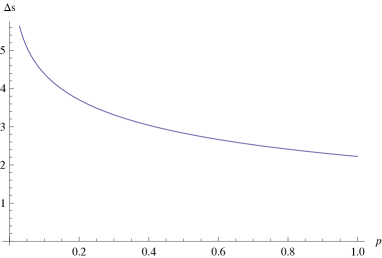
the area is given by the integral
| (71) |
where the limit is understood, and we have defined191919The elliptic integrals of the first, second and third kind with argument , modulus and parameter are denoted by , , respectively. When the argument is omitted and is denoted by . To agree with the conventions of int , we should replace and exchange .
| (72) |
Since these integrals are finite for every allowed value of , in this form the divergence coming from is manifest. However, it is exactly the area divergence of the disconnected solution and then the difference
| (73) |
is well defined202020The same result is obtained by performing the Legendre transform. for every fixed .
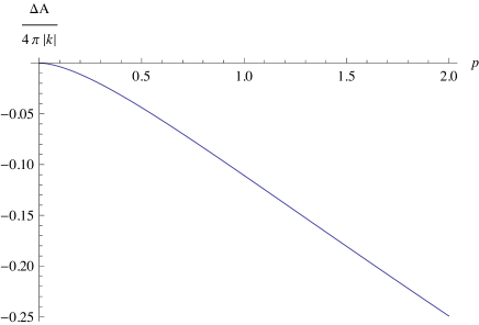
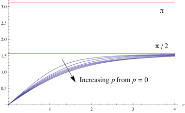
From the plot shown in Fig.3, we can see that the connected surface has smaller area than the disconnected one for any (): the connected solution always dominates. For , diverges: as shown below, this corresponds to the limit of coincident fibers.
From (63) we can see that the parameter is related to the boundary conditions on the angular coordinates of . In order to make everything as simple as possible212121Actually, the general case is straightforward. In fact, upon the use of the second Virasoro constraint, the parameter can be related to the geodesic (or Euclidean) distance of the fibers on the base, which can be expressed in terms of ., we can consider the particular solution with (and hence also ). In this case each fiber is identified uniquely by , which is in turn determined by (assuming )
| (74) |
Therefore
| (75) |
The limit yields the boundary values of , that is the fiber positions on the base : if on the negative branch we set , while on the positive one, we have
| (76) |
which is indeed a (non-trivial) relation between the angular separation of the boundary fibers and the parameter . The integral above can be evaluated explicitly and we get (with the same notations as before)
| (77) |
where
| (78) |
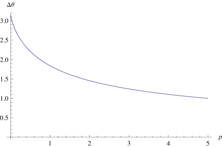
From the plot in Fig.4, we can see that at the maximal meaningful separation () we have a disconnected solution (). The other limit corresponds to coincident fibers. In a sense, there is a sort of continuous222222We mean that the disconnected solution can be continuously obtained from the connected one by going continuously from to . As we will explain, this corresponds to a BPS/non-BPS transition. “phase transition” at . A similar phenomenon occurs in the correlator of two parallel and concentric circles (Gross-Ooguri phase transition). However, in that case it exists a region where the connected solution has area bigger than the disconnected one, and beyond a certain separation it ceases even to exist. In our case this situation never happens.
From (66) it follows that the implicit form of is given by
| (79) |
where represents the turning point , . The range of the parameter can be determined by taking the limit
| (80) |
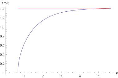
This is shown in Fig.5. For the range diverges, corresponding to the fact that the turning point is mapped to the deep interior of . Actually, describes the disconnected solution.
III.4 Motion in
We will now consider what happens when we allow an motion, namely when . From (66) we can see that the area (69) is simply replaced by
| (81) |
where is the unique real positive zero of the square root as determined in (65). By setting
| (82) |
the area is given as in (71), (72) but with the replacements , . In the following we must be careful about the range of the parameter : in fact, it is determined by the equation, but it is also the parameter of the motion. From (66) we get
| (83) |
where and
| (84) |
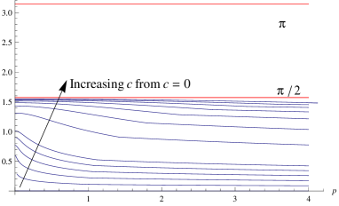
The parameters and are not independent of each other. Rather, they must satisfy a compatibility condition. In fact, when the fibers have the same (opposite) scalar charge (40) they sit on the same (antipodal) point(s) of at the AdS boundary. Since we have considered an motion given by (41)
| (85) |
we must have (), where represent the boundary values of the angle. Then the compatibility condition
| (86) |
must be satisfied. We remark that it is a very strong constraint on the full motion, and it turns out there is no solution other than , as shown in Fig.6. As a matter of fact, the function on the left-hand side of (86) reaches the minimum required value only asymptotically for . We conclude that there exists no connected solution for two antiparallel Hopf fibers of opposite scalar charge (at least as far as the made ansatz is concerned).
So far, the study of the Hopf fiber correlator has been (almost) purely geometrical, and this is motivated by the AdS/CFT geometric prescription to calculate Wilson loop expectation values. However, the string dual of a supersymmetric system of DGRT loops is expected to be represented by a supersymmetric string surface, and then the surface has to be a solution of the sigma model as well as of the -symmetry equations. In the following section we are going to explore this issue for the connected solution, and we will show that it is not supersymmetric.
IV Supersymmetry
In order to verify whether the found solution is a supersymmetric string surface dual to a correlator of two DGRT Hopf fibers, we follow an argument proposed in dgrta (see also Dymarsky:2009si for a general discussion). We will be rather sketchy, and we will refer to that paper and references therein for details.
In the –symmetry equations read as
| (87) |
where are the 10-dimensional curved space gamma matrices, is the 2-dimensional antisymmetric tensor and is the conformal Killing spinor.
To check the supersymmetry of the connected solution, we should plug it into (87). However, there is a simpler way to perform such a verification. Let us consider the following equations
| (88) |
where is the canonical complex structure associated to the world-sheet metric and is a certain matrix defined in the subspace where the solution lives232323We remind that .. It defines an almost complex structure (), and represents an elegant way to collect the BPS properties of DGRT loops. A surface extending into and satisfying defines a pseudo-holomorphic surface with respect to . Since is related to the BPS nature of DGRT loops, dual string surfaces are expected to be compatible with it, i.e. pseudo-holomorphic with respect to . In support of this conjecture, in dgrta it has been shown that classical pseudo-holomorphic string surfaces are automatically supersymmetric: we are interested in verifying whether the found string solution is pseudo-holomorphic. Taking the explicit form of as given in dgrta (rewritten in terms of the coordinates we have employed), we can plug the given ansatz into the pseudo-holomorphic equations (88), and the resulting independent conditions turn out to be
| (89) |
We can recognize the equations associated to the 1/2 BPS circular loop () and the second Virasoro constraint, which is however automatically satisfied by the requirement . Thus the pseudo-holomorphic equations single out the disconnected solution242424We have verified that the same result can be directly obtained from the –symmetry equations..
We observe that the connected string solution we found is not describing the connected correlator of two DGRT Hopf fibers: the non-supersymmetric nature of the solution can be traced back to a “wrong” relative orientation of the boundary circles. To see this, let us come back to the definition of a DGRT loop (3)
| (90) |
When is a Hopf fiber (10) parameterized by , the above operator becomes
| (91) |
because (with the conventions of the previous sections)
| (92) |
In considering the correlator of two Hopf fibers, the BPS configurations involve equally oriented fibers with the same scalar charge, or oppositely oriented fibers of opposite scalar charge. This observation suggests that our non-BPS connected string solution describes the correlator of two oppositely oriented Hopf fibers with the same scalar charge.
In fact, the non-supersymmetric connected solution is characterized by having no motion in , implying that the fibers have the same scalar charge. Moreover, the tangential direction and the radial direction252525. along one fiber on the AdS boundary define an orientation that must be preserved along the world-sheet. However, in the two different radial branches the sign of is opposite, and hence also the sign of the tangential vector has to be reversed to keep the orientation. We get the picture of a pair of antiparallel Hopf fibers with the same scalar charge.
Interestingly enough, our solution is able to interpolate between a BPS configuration and a non-BPS one. We saw that for general values of (or ) the string surface is not supersymmetric, but for (or ) the solution approaches the disconnected one made of a pair of surfaces which are separately BPS (single great circle). When considered together, one surface halves the preserved supersymmetries of the other, giving rise to a BPS configuration. This situation can be easily understood from the gauge theory viewpoint: the fibers at and lay on the plane and respectively. Each loop represents the BPS great circle, and the presence of a second circle in the orthogonal plane simply halves the components of the independent supersymmetric spinor by imposing a chirality condition. The explicit calculation can be found in dgrta for the case of two DGRT parallel fibers, but the same applies also to the non-DGRT antiparallel fibers in the special case , , since the supersymmetry variation becomes insensible 262626The only difference is a flip of the chirality. to the “wrong” sign of the charges.
V Quark-antiquark static potential
The connected solution we have found represents a system made of a pair of antiparallel fibers, with the same scalar charge: in some sense, it can be thought of as a topologically non-trivial analogue in of the antiparallel lines describing the static quark-antiquark potential. In fact, when the fibers are sufficiently close to each other (namely , or ), locally they look like straight antiparallel lines. In this picture, we can expect that the role of the separation distance between the lines in the (strong coupling) static potential pot1 ; mwloop
| (93) |
will be played by (in the large limit), the distance between the Hopf fibers on the base in the metric. This will indeed be the case.
There is a subtle point in this interpretation: while the two antiparallel lines are thought as a degenerate rectangular single loop of infinite extension, involving only one trace, we are dealing here with the correlator of two loops, involving two different traces. The precise relation between the two quantities is well known, involving the physical interpretation of the different loop correlators in terms of singlet and adjoint potentials Brown:1979ya ; Nadkarni .
A quark-antiquark pair at the same point can be in either a singlet or an adjoint state, according to the irreducible representations of the tensor product
| (94) |
The usual strategy to extract the quark-antiquark potential from Wilson loop is to relate the four point function (in the infinite mass limit)
| (95) |
to the gauge invariant phases, experienced by the fields ’s in their temporal evolution, as . Here are placed at while at (see Brown:1979ya ; Nadkarni for further details). The field has a color index and the general structure of the correlation function in the large limit, taking and , is
| (96) |
The matrix operators and project respectively onto the singlet state and the adjoint state, according to the decomposition (94). By taking the relevant traces with the projectors and relating the four-point functions to correlators of Wilson lines we get the following identities:
| (97) |
and
| (98) |
being the Wilson line in extending along the Euclidean time. The first relation is the familiar definition of the quark-antiquark potential in terms of antiparallel Wilson lines. The second equality gives us instead a physical interpretation of the correlator two traced Wilson lines, in terms of the singlet and adjoint potential . Using the explicit definition of the singlet potential we finally arrive at
| (99) |
that expresses the normalized connected correlator of the two traced Wilson lines in terms of the potentials. This is the key relation to derive the quark-antiquark potential, in the limit of small separation between the fibers, from the DGRT loops correlator both at weak and strong coupling.
We proceed as follows: assuming for an expansion in powers of , we have up to the second order in
| (100) | ||||
| (101) |
In order to keep track of the powers of , we set , and , so that and and the (101) becomes
| (102) |
The solution to this equation can be written as a power series of
| (103) |
and, in the large limit, we can expand in power of finding
| (104) |
This simple result shows that if we want to compute the order of the static potential, we need the order for the correlator of Wilson loops. However, the technical difficulties in computing Feynman graphs allows only for numerical computations, as in the case of twotwo . We will not attempt this computation and we will only check the leading order result.
At strong-coupling, due to the exponentiation property of the Wilson loops correlator, we can directly relate our string solution with the singlet potential: let us compute the relevant quantities in the large limit. The regularized area (73) becomes
| (105) |
and in the same limit the angular separation (77) approaches
| (106) |
obtaining
| (107) |
Since
| (108) |
we naturally define
| (109) |
where is the length of the fiber in the metric. We see immediately that
| (110) |
which, as expected, coincides with the function once we identify .
VI Conclusions
In this paper we have studied at string level the correlator of two Wilson loops involving Hopf fibers of in SYM theory. The system has been originally introduced in the context of Wilson loops in dgrta , and it represents an example of topologically non-trivial loop configuration. Our main motivation for the study of such a system was indeed to explore non-trivial topologies, and to continue the analysis of configurations involving circles. The study has been performed at strong-coupling, using AdS/CFT correspondence, and we have been able to find a connected string surface linking the two boundary fibers. It has been shown that the solution describes the connected correlator of a pair of antiparallel Hopf fibers with the same scalar charge. For this reason, we have observed that such a system can be thought of as a deformation of the ordinary antiparallel lines describing the static quark-antiquark potential. Indeed, we have verified at weak and strong coupling that the latter system is recovered in the small separation limit, once the fiber distance is identified with distance between the lines. We observed an interesting dynamics, where the string solution is able to continuously interpolate between a non-BPS configuration and a BPS one by varying a parameter.
Moreover, our analysis suggests that the correlator of two antiparallel DGRT Hopf fibers does not admit a connected string solution, and presumably the parallel ones neither. Of course, this is certainly true as far as the considered type of solution is concerned, but it provides by no means a general proof. We can only observe that the our ansatz is the most natural and minimal one with respect to the Hopf fibration geometry: it seems very difficult to construct an inevitably more complicated solution respecting the desired boundary conditions. This fact may be considered as a string theory result in favor of the exactness of the matrix model for two DGRT fibers. It would be interesting, of course, to check this expectation directly in the gauge theory side at higher order in perturbation theory.
Another interesting direction worth to be studied is the application of the found string solution to the holographic calculation of the 3-point correlation function of semiclassical states and non-BPS operators jsw ; zarembo ; Costa:2010rz . Even though a precise string description of such observables is still a long way off, recently the problem has been faced in the simplified version of considering the correlator of two heavy operators and a light one. In some cases two Wilson loops have been considered as the heavy operators aldaytseytlin , and then the semiclassical computation of the 3-point function amounts to evaluate the string vertex operator of the light operator over the classical world-sheet generated by the heavy ones. For such calculations an explicit and analytical expression of the classical string solution is needed, but only few are known. In this paper we have presented a new type of solution, and thus it can be used in that context. We defer this possibility to future investigations.
Acknowledgements
This work was supported in part by the MIUR-PRIN contract 2009-KHZKRX. We thank Nadav Drukker for illuminating discussions and Donovan Young for sharing with us his perturbative results.
Appendices
Appendix A Explicit form of the solution
For completeness, we report here the explicit form of the functions , , , . From (79) we have
| (A.113) |
where
| (A.114) |
Therefore272727, , .
| (A.115) |
We see that it is much more convenient to express all the variables as functions of282828Reminding the relation between global and Poincaré coordinates ) of one can also easily trade for . . As far as the angular variables are concerned, we start from the case . From (75) we get
| (A.116) |
where
| (A.117) |
and the value at the turning point corresponds to the mean value .
As observed in Section II, in principle it is possible to work with . In this case, the relevant equations are (55), (56) (we take )
| (A.118) |
and (66)
| (A.119) |
Consistency requires , , and the extremum () is taken in correspondence of (). Assuming it is located at , from (A.118) it follows
| (A.120) |
In the case , the expression (A.116) is recovered (except for the integration constant, which does not represent any extremum for ). For , the left-hand side of (A.120) is not well defined. However, from (A.118) we can realize that it is consistent to consider , , and then , simply exchange the roles with respect to the case .
Now that is known, the , equations can be easily integrated
| (A.121) |
We conclude by observing that there is another derivative that can be turned on, namely . Throughout the paper we have considered , and this is motivated by the fact that we wanted to consider fibers on the same 3-sphere. Therefore, on the AdS boundary, has to be the same for the two fibers, and the simpler way to guarantee this is indeed to set .
Appendix B Perturbative calculations
We present here the perturbative expansion, up to order , of the connected correlator of two antiparallel Hopf fibers () of equal scalar charge (). The parameters along the two fibers will be denoted by and , , while points will be denoted by and . Reminding the general expression of the propagator (7), evaluating it on different fibers292929Due to the relation between the orientation and the scalar charge, the propagator is no longer constant. we get
| (B.122) |
where , , , while
| (B.123) |
when the points belong to the same fiber. In the following we are going to consider the particular solution , so that the expression above simplifies to
| (B.124) |
As far as the gauge group generators are concerned, we follow the conventions of twotwo
| (B.125) |
Order .
The only contribution is from the single exchange diagram
| . |
Since
| (B.126) |
and
| (B.127) |
we get
| (B.128) |
Order .
There are two inequivalent diagrams
| , | |
| . |
Since
| (B.129) |
we get
| (B.130) |
and
| (B.131) |
Let us conclude by observing that it is possible to work also with . In fact, in this case
| (B.132) |
where is the Euclidean distance between two points , on the base . We can see that (B.127) corresponds indeed to .
References
- (1) W. J. Rey and J. T. Yee, “Macroscopic strings as heavy quarks in large N gauge theory and anti-de Witter supergravity,” Eur. Phys. J. C 22, 379 (2001) [arXiv:hep-th/9803001].
- (2) J. M. Maldacena, “Wilson loops in large N field theories,” Phys. Rev. Lett. 80, 4859 (1998) [arXiv:hep-th/9803002].
- (3) N. Drukker, D. J. Gross and H. Ooguri, “Wilson loops and minimal surfaces,” Phys. Rev. D 60, 125006 (1999) [hep-th/9904191].
- (4) K. Zarembo, “Supersymmetric Wilson loops,” Nucl. Phys. B 643, 157 (2002) [arXiv:hep-th/0205160].
- (5) N. Drukker, S. Giombi, R. Ricci and D. Trancanelli, “Supersymmetric Wilson loops on ,” JHEP 0805, 017 (2008) [arXiv:0711.3226 [hep-th]]. jhep05(2008)017.
- (6) J. K. Erickson, G. W. Semenoff and K. Zarembo, “Wilson loops in N=4 supersymmetric Yang-Mills theory,” Nucl. Phys. B 582 (2000) 155 [hep-th/0003055].
- (7) N. Drukker and D. J. Gross, “An Exact prediction of N=4 SUSYM theory for string theory,” J. Math. Phys. 42, 2896 (2001) [arXiv:hep-th/0010274].
- (8) V. Pestun, “Localization of gauge theory on a four-sphere and supersymmetric Wilson loops,” arXiv:0712.2824 [hep-th].
- (9) D. Young, “BPS Wilson Loops on at Higher Loops,” JHEP 0805, 077 (2008) [arXiv:0804.4098 [hep-th]].
- (10) A. Bassetto, L. Griguolo, F. Pucci and D. Seminara, “Supersymmetric Wilson loops at two loops,” JHEP 0806, 083 (2008) [arXiv:0804.3973 [hep-th]].
- (11) S. Giombi, V. Pestun and R. Ricci, “Notes on supersymmetric Wilson loops on a two-sphere,” JHEP 1007 (2010) 088 [arXiv:0905.0665 [hep-th]].
- (12) A. Bassetto, L. Griguolo, F. Pucci, D. Seminara, S. Thambyahpillai and D. Young, “Correlators of supersymmetric Wilson-loops, protected operators and matrix models in N=4 SYM,” JHEP 0908, 061 (2009) [arXiv:0905.1943 [hep-th]].
- (13) A. Bassetto, L. Griguolo, F. Pucci, D. Seminara, S. Thambyahpillai and D. Young, “Correlators of supersymmetric Wilson loops at weak and strong coupling,” JHEP 1003, 038 (2010) [arXiv:0912.5440 [hep-th]].
- (14) S. Giombi and V. Pestun, “Correlators of local operators and 1/8 BPS Wilson loops on S**2 from 2d YM and matrix models,” JHEP 1010 (2010) 033 [arXiv:0906.1572 [hep-th]].
- (15) V. Pestun, “Localization of the four-dimensional N=4 SYM to a two-sphere and 1/8 BPS Wilson loops”, arXiv:0906.0638 [hep-th].
- (16) A. Dymarsky and V. Pestun, “Supersymmetric Wilson loops in N=4 WYM and pure spinors,” JHEP 1004, 115 (2010) [arXiv:0911.1841 [hep-th]].
- (17) V. Cardinali, L. Griguolo and D. Seminara, “Impure Aspects of Supersymmetric Wilson Loops,” arXiv:1202.6393 [hep-th].
- (18) M. Kruczenski and A. Tirziu, “Matching the circular Wilson loop with dual open string solution at 1-loop in strong coupling,” JHEP 0805 (2008) 064 [arXiv:0803.0315 [hep-th]].
- (19) F. Passerini and K. Zarembo, “Wilson Loops in N=2 Super-Yang-Mills from Matrix Model,” JHEP 1109 (2011) 102 [Erratum-ibid. 1110 (2011) 065] [arXiv:1106.5763 [hep-th]].
- (20) J. K. Erickson, G. W. Semenoff, R. J. Szabo and K. Zarembo, “Static potential in N=4 supersymmetric Yang-Mills theory,” Phys. Rev. D 61 (2000) 105006 [hep-th/9911088].
- (21) A. Pineda, “The Static potential in N = 4 supersymmetric Yang-Mills at weak coupling,” Phys. Rev. D 77 (2008) 021701 [arXiv:0709.2876 [hep-th]].
- (22) S. -x. Chu, D. Hou and H. -c. Ren, “The Subleading Term of the Strong Coupling Expansion of the Heavy-Quark Potential in a N=4 Super Yang-Mills Vacuum,” JHEP 0908, 004 (2009) [arXiv:0905.1874 [hep-ph]].
- (23) V. Forini, “Quark-antiquark potential in AdS at one loop,” JHEP 1011, 079 (2010) [arXiv:1009.3939 [hep-th]].
- (24) N. Drukker and V. Forini, “Generalized quark-antiquark potential at weak and strong coupling,” JHEP 1106 (2011) 131 [arXiv:1105.5144 [hep-th]].
- (25) D. Correa, J. Henn, J. Maldacena and A. Sever, “An exact formula for the radiation of a moving quark in N=4 super Yang Mills,” arXiv:1202.4455 [hep-th].
- (26) D. Correa, J. Maldacena and A. Sever, “The quark anti-quark potential and the cusp anomalous dimension from a TBA equation,” arXiv:1203.1913 [hep-th].
- (27) N. Drukker, “Integrable Wilson loops,” arXiv:1203.1617 [hep-th].
- (28) D. J. Gross and H. Ooguri, “Aspects of large N gauge theory dynamics as seen by string theory,” Phys. Rev. D 58 (1998) 106002 [hep-th/9805129].
- (29) J. Plefka and M. Staudacher, “Two loops to two loops in N=4 supersymmetric Yang-Mills theory,” JHEP 0109 (2001) 031 [hep-th/0108182].
- (30) G. Arutyunov, J. Plefka and M. Staudacher, “Limiting geometries of two circular Maldacena-Wilson loop operators,” JHEP 0112 (2001) 014 [hep-th/0111290].
- (31) K. Zarembo, “Wilson loop correlator in the AdS / CFT correspondence,” Phys. Lett. B 459 (1999) 527 [hep-th/9904149].
- (32) P. Olesen and K. Zarembo, “Phase transition in Wilson loop correlator from AdS / CFT correspondence,” hep-th/0009210.
- (33) D. Young Private Communication.
- (34) Metsaev R.R., Tseytlin A.A., “Type IIB superstring action in background”, arXiv:hep-th/9805028, 1998.
- (35) Drukker N., Fiol B., “On the integrability of Wilson loops in : Some periodic ansatze”, arXiv:hep-th/0506058v1, 2005.
- (36) Okuyama K., “Global AdS Picture of 1/2 BPS Wilson Loops”, arXiv:hep-th/0912.1844v3, 2010.
- (37) Gradshteyn I.S., Ryzhik I.M. “Table of Integrals,Series, and Products”, 6th ed., Academic Press, 2000.
- (38) L. S. Brown and W. I. Weisberger, “Remarks On The Static Potential In Quantum Chromodynamics,” Phys. Rev. D 20, 3239 (1979).
- (39) Nadkarni, “Nonabelian Debye Screening. 2. The Singlet Potential.” Phys. Rev. D 34 (1986) 3904.
- (40) Janik R.A., Sur wka P., Wereszczynski A., “On correlation functions of operators dual to classical spinning string states”, arXiv:hep-th/1002.4613v2, 2010.
- (41) Zarembo K., “Holographic three-point functions of semiclassical states”, arXiv:hep-th/1008.1059v3, 2010.
- (42) M. S. Costa, R. Monteiro, J. E. Santos and D. Zoakos, “On three-point correlation functions in the gauge/gravity duality,” JHEP 1011, 141 (2010) [arXiv:1008.1070 [hep-th]].
- (43) Alday L.F., Tseytlin A.A., “On strong-coupling correlation functions of circular Wilson loops and local operators”, arXiv:hep-th/1105.1537v2, 2011.