GLOBAL AND PARTIAL PHASE SYNCHRONIZATIONS IN ARRAYS OF PIECEWISE LINEAR TIME-DELAY SYSTEMS

Abstract

In this paper, we report the phenomena of global and partial phase synchronizations in linear arrays of unidirectionally coupled piecewise linear time-delay systems. In particular, in a linear array with open end boundary conditions, global phase synchronization (GPS) is achieved by a sequential synchronization of local oscillators in the array as a function of the coupling strength (a second order transition). Several phase synchronized clusters are also formed during the transition to GPS at intermediate values of the coupling strength, as a prelude to full scale synchronization. On the other hand, in a linear array with closed end boundary conditions (ring topology), partial phase synchronization (PPS) is achieved by forming different groups of phase synchronized clusters above some threshold value of the coupling strength (a first order transition) where they continue to be in a stable PPS state. We confirm the occurrence of both global and partial phase synchronizations in two different piecewise linear time-delay systems using various qualitative and quantitative measures in three different framework, namely, using explicit phase, recurrence quantification analysis and the framework of localized sets.

1 Introduction

Chaotic phase synchronization (CPS) associated with a locking of the phases of coupled chaotic systems corresponds to the case where the amplitudes are still uncorrelated. CPS has been investigated in ensembles of globally coupled arrays Pikovsky et al. [2001]; Boccaletti et al. [2002]; Ivanchenko et al. [2004]; Takamatsu et al. [2000]; Pikovsky et al. [1996]; Kiss et al. [2001]; Zhou et al. [2002]; Osipov et al. [1997]; Zhan et al. [2000]; Kozyreff et al. [2000]; Otsuka et al. [2006], networks of oscillators Boccaletti et al. [2006]; Arenas et al. [2008]; Batista et al. [2007]; Ren & Zhao [2007]; Yu et al. [2009], laser systems Kozyreff et al. [2000]; Otsuka et al. [2006], cardiorespiratory systems Schafer et al. [1998]; Stefanovska et al. [2000]; Bartsch et al. [2007], ecology Blasius et al. [1999]; Sismondo [1990]; Amritkar & Rangarajan [2006], climatology Rybski et al. [2006]; Yamasaki et al. [2009]; Maraun et al. [2005], etc. CPS is well studied and understood in low dimensional systems; however, there exist a very little indepth studies in higher dimensional systems such as time-delay systems, which are essentially infinite-dimensional and exhibit highly non-phase-coherent hyperchaotic attractors with complex topological structures. So estimating the phase explicitly to identify phase synchronization in such systems is quite difficult. Recently, the occurrence of phase synchronization in time-delay systems has been reported Senthilkumar et al. [2006, 2008]. However, these investigations are carried out so far only in a system of two coupled time-delay systems. Very recently, the occurrence of global phase synchronization in a linear array of Mackey-Glass time-delay systems in the chaotic regime has been reported in Suresh et al., [2010] for open end boundary conditions. It has been shown that global phase synchronization occurs via a sequential type synchronization as the coupling strength increases. To verify the generic nature of the results of Suresh et al., [2010], we consider in this paper two different piecewise linear time-delay systems with complex topological structures and investigate the occurrence of global phase synchronization along with the underlying mechanism for open end boundary conditions. In addition we consider the case of closed end boundary conditions (ring topology) and identify the occurrence of partial phase synchronization via cluster formation.

Specifically, in the first part of this paper, we investigate the generic nature of the phenomenon of global phase synchronization in an linear array, with free ends, of unidirectionally coupled (i) piecewise linear and (ii) threshold nonlinear time-delay systems in hyperchaotic regimes. In the second part, we report the phenomena of partial phase synchronizations in the array of above two systems but with closed end boundary conditions. At first, we use the nonlinear transformation introduced in Senthilkumar et al., [2006, 2008] to estimate the phase of all the systems in the array and to identify the existence of phase synchronization. Further, we confirm the existence of global phase synchronization (GPS) and partial phase synchronization (PPS) from the original non-phase-coherent hyperchaotic attractors using two independent approaches, namely recurrence quantification analysis Romano et al. [2005]; Marwan et al. [2007] and the concept of localized sets Pereira et al. [2007]. In addition, we point out that the onset of GPS in the linear array with open end boundary conditions takes place in the form of a sequential synchronization (second order transition): For lower values of coupling strength the phases of nearby systems get already entrained with the drive system in contrast to the far away systems, while the other non-synchronized systems display clusters of phase synchronized states among themselves before they become synchronized with the large cluster in the sequence as the strength of coupling increases to form the GPS.

On the other hand, if we consider an array with closed end boundary conditions (ring topology), partial phase synchronization occurs with the formation of different groups of phase synchronized clusters. The oscillators in the array self-organize to form groups of phase synchronized clusters where each cluster is in perfect phase synchrony as a function of the coupling strength. Such a clustering is considered to be particularly significant in biological systems Kaneko [1990]; Sherman [1994]; Strogatz & Stewart [1993], in electro-chemical oscillators Kiss et al. [2001], etc. Recently, cluster synchronization in an array of three chaotic lasers without delay was reported Terry et al. [1999] as well. In our case, as the coupling strength increases, every individual system starts to drive the nearest system and the systems with small differences in their phases organize themselves to form small groups of clusters leaving the other oscillators with large phase differences to evolve independently. Further increase in the coupling strength results in an increase in the sizes of the clusters due to the locking of the phases of the nearby oscillators of the clusters for appropriate values of the coupling strength and finally ending up with large groups of clusters resulting in PPS (first order transition).

The paper is organized as follows: In Secs. 3 and 4, we will describe briefly the coupling configuration and the occurrence of global phase synchronization in an array of two different piecewise linear time-delay systems with open end boundary conditions. In Secs. 5 and 6 we consider the linear array of two piecewise linear time-delay systems with closed end boundary conditions (ring topology) and discuss the occurrence of partial phase synchronization and finally we summarize our results in Sec. 7.

Figure 1: Attractors of the piecewise linear system. (a) non-phase-coherent hyperchaotic attractor of the drive system (4a). (b) Transformed attractor of the drive system. (c-f) Transformed attractors of some of the uniformly selected response systems ($i=10,20,30,50$) in the new state space ($x_{i}(t+\tau),z_{i}(t+\tau)$).

2 Estimates of phase

Identifying Chaotic phase synchronization is a nontrivial problem in time-delay systems exhibiting complicated hyperchaotic attractors. For this purpose one requires appropriate measures. In this section, we describe briefly the various measures which we used from three different frameworks in this paper to estimate the phase of time-delay systems thereby facilitating the characterization of phase synchronization between the coupled time-delay systems.

2.1 Transformation of the original non-phase-coherent attractor

Time-delay systems usually exhibit a highly complicated non-phase-coherent chaotic/hyperchaotic attractor with their flows having more than a single center of rotation. Such an attractor does not yield a monotonically increasing phase on estimating it using the conventional techniques Senthilkumar et al. [2006, 2008]. For this purpose, we have introduced a nonlinear transformation to recast the original non-phase-coherent attractor into a smeared limit cycle-like attractor with a single center of rotation. Our transformation is obtained by defining a new state variable Senthilkumar et al. [2006, 2008],

$$z(t+\tau)=x(t)x(t+\hat{\tau})/x(t+\tau),$$ (1)

where $\hat{\tau}$ is the optimal value of time-delay to be chosen in order to avoid any additional center of rotation. Then, the projected trajectory in the transformed state space ($x(t+\tau),z(t+\tau)$) will resemble that of a smeared limit cycle-like attractor. Such an approach facilitates the estimation of phase from the conventional techniques.

2.2 Recurrence quantification analysis

Several measures of complexity quantifying the small scale structures in recurrence plots have been proposed and the corresponding description is known as recurrence quantification analysis (RQA) Marwan et al. [2007]. In addition to the other advantages of the RQA such as its application to short experimental data, nonstationary and noisy data, we find that it can also be applied directly to highly complicated non-phase-coherent attractors of the time-delay systems in characterizing the synchronization transitions, in particular phase synchronization (PS) transitions. Among the available recurrence quantification measures, we use the Correlation of Probability of Recurrence (CPR) and the generalized autocorrelation function $P(t)$, which are estimated from the original non-phase-coherent hyperchaotic attractors, to confirm the existence of GPS in the array of coupled time-delay systems, both qualitatively and quantitatively.

A criterion to quantify phase synchronization between two systems is the Correlation of Probability of Recurrence (CPR) defined as

$$CPR=\langle\bar{P_{1}}(t)\bar{P_{2}}(t)\rangle/\sigma_{1}\sigma_{2},$$ (2)

where $P(t)$ is the recurrence-based generalized autocorrelation function defined as

$$P(t)=\frac{1}{N-t}\sum_{i=1}^{N-t}\Theta(\epsilon-||X_{i}-X_{i+t}||),$$ (3)

where $\Theta$ is the Heaviside function, $X_{i}$ is the $i^{th}$ data point of the system $X$, $\epsilon$ is a predefined threshold, $||.||$ is the Euclidean norm, and $N$ is the number of data points, $\bar{P}_{1,2}$ means that the mean value has been subtracted and $\sigma_{1,2}$ are the standard deviations of $P_{1}(t)$ and $P_{2}(t)$, respectively. Looking at the coincidence of the positions of the maxima of $P(t)$ of the coupled systems, one can qualitatively identify PS Romano et al. [2005]; Marwan et al. [2007]. If both systems are in CPS, the probability of recurrence is maximal at the same time $t$ and CPR $\approx 1.0$. If they are not in CPS, the maxima do not occur simultaneously and hence one can expect a drift in both probabilities of recurrences resulting in low values of CPR.

2.3 The concept of localized sets

Another measure that we have employed is the framework of localized sets Pereira et al. [2007]. The concept of localized sets opens up the possibility of an easy and an efficient way to detect CPS especially in complicated non-phase-coherent attractors of time-delay systems. The main ingredient of this technique is to define an event in one of the systems and then observe the other during the event, which defines a set $D$. Depending upon the property of this set $D$, one can state whether PS exists or not. The set is spread over the entire attractor for asynchronous systems, whereas it is localized on the attractor if the coupled systems are mutually phase-locked or in phase synchronous state.

We use the above three different frameworks to confirm the existence of GPS in an array of piecewise linear time-delay systems in the following.

3 GPS in a Linear Array of Time-delay Systems with piecewise linearity

Recently, we have reported the dynamical organization of an array of Mackey-Glass time-delay systems in chaotic regime to form global phase synchronization (GPS) via sequential synchronization Suresh et al. [2010], as mentioned in the introduction. In this section, we intend to examine the generic nature of the results in Ref. Suresh et al. [2010], by investigating the emergence of GPS in an array of a particular type of piecewise linear time-delay systems from the local sequential synchronization as the coupling strength is increased from zero to that of the hyperchaotic regimes. It is worth to emphasize that the hyperchaotic attractors of the piecewise linear time-delay systems are characterized by much more complex topological properties than the chaotic attractor of the Mackey-Glass time-delay system studied in  Suresh et al. [2010] and so is of considerable significance in estimating the onset of GPS through sequential synchronization.

3.1 Linear array of piecewise linear time-delay systems

Now, we consider an array of unidirectionally coupled piecewise linear time-delay systems with open end boundary conditions and with parameter mismatches. Linear stability and bifurcation analysis of this system has been well studied in Ref. Lakshmanan & Senthilkumar [2010]; Senthilkumar & Lakshmanan [2005]. Many kind of synchronizations and their transitions have been reported in the coupled piecewise linear time-delay systems Senthilkumar & Lakshmanan [2005, 2007]; Lakshmanan & Senthilkumar [2010]. The array of unidirectionally coupled piecewise linear first-order delay differential equations is represented as

$$\dot{x}_{1}(t) = -\beta x_{1}(t)+\alpha_{1}f(x_{1}(t-\tau)),$$ (4a)

$$\dot{x}_{i}(t) = -\beta x_{i}(t)+\alpha_{i}f(x_{i}(t-\tau))+\varepsilon(x_{i-1}(t)-x_{i}(t)),\quad i=2,3,\cdots,N,$$ (4b)

where $\alpha,\beta$ are the system parameters, $\tau$ is the time-delay and $\varepsilon$ is the coupling strength. We use the open end boundary conditions $x_{0}=x_{1}$ and $x_{N}=x_{N-1}$. The nonlinear function $f(x)$ is chosen to be a piecewise linear function defined as

$$f(x)=\left\{\begin{array}[]{cc}0,&x\leq-4/3\\ -1.5x-2,&-4/3<x\leq-0.8\\ x,&-0.8<x\leq 0.8\\ -1.5x+2,&-0.8<x\leq 4/3\\ 0,&x>4/3.\end{array}\right.$$ (10)

Figure 2: Plot of the first ten maximal Lyapunov exponents $\lambda_{max}$ of the piecewise linear time-delay system (4a) for the parameter values $\beta=1.0$, $\alpha_{1}=1.2,\tau\in(3,25)$.

The system parameters are fixed as follows: $\beta=1.0$, $\alpha_{1}=1.2$, $\tau=15.0$. The values of the nonlinear parameter $\alpha_{i}$ of the response systems in the array are chosen randomly in the range $\alpha_{i}\in(1.19,1.23)$, so that all the subsystems are effectively nonidentical due to the parameter mismatch. The original non-phase-coherent hyperchaotic attractor of the drive in the $(x(t),x(t-\tau))$ state space is illustrated in Fig. 1(a). The corresponding transformed attractor, effected using the transformation (1), in the new state space ($x(t+\tau),z(t+\tau)$) is depicted in Fig. 1 (b), which now looks like a smeared limit cycle-like attractor with a single center of rotation. The optimal value of the $\hat{\tau}$ in (1) for the above piecewise linear time-delay systems is found to be 1.6 Senthilkumar et al. [2006]. The same transformation has also been performed for the non-phase-coherent chaotic attractor of the Mackey-Glass time-delay system with an appropriate $\hat{\tau}$ in Ref. Suresh et al. [2010]. The hyperchaotic nature of the attractor in Figs. 1 for the above parameter values is confirmed from three positive Lyapunov exponents at $\tau=15.0$ in the spectrum of ten maximal Lyapunov exponents of (4a) as a function of the time-delay parameter $\tau\in(3,25)$ in Fig. 2.

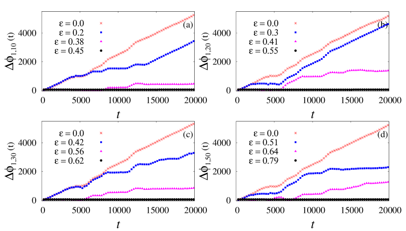
Figure 3: (a-d) Plots of the phase differences ($\Delta\phi_{1,i}$ = $\phi_{1}-\phi_{i}$) of some of the selected systems ($i$ = 10, 20, 30, 50) in the array for different $\varepsilon$.

3.2 Identification of GPS from the transformed attractor of the piecewise linear time-delay system

To confirm the existence of GPS in the array of piecewise linear time-delay systems, we have fixed size of the array as $N=50$. The transformed smeared limit cycle-like attractors with a single center of rotation of some of the uniformly selected subsystems ($i$ = 10, 20, 30, 50) in the linear array are shown in Figs. 1 (c-f). We have used the conventional Poincaré section technique Pikovsky et al. [2001]; Boccaletti et al. [2002] to estimate the instantaneous phases of all the oscillators after the transformation of the attractors, which now yields monotonically increasing phase. Open circles in Figs. 1(b-f) indicate the Poincaré section.

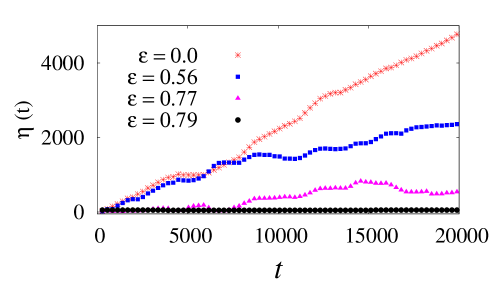
Figure 4: The evolution of the average phase difference [$\eta(t)$] for different values of the coupling strength $\varepsilon$.

In the absence of coupling ($\varepsilon=0.0$) between the piecewise linear time-delay systems in the array, the individual subsystems evolve independently in an asynchronous fashion which is indeed confirmed from the monotonous increase in the phase differences, $\Delta\phi_{i}=\phi_{1}-\phi_{i}$, between the drive and the uniformly selected response systems ($i=10,20,30,50$) indicated by asterisk symbols in Figs. 3. Phase slips (marked by filled squares and triangles) in Figs. 3 for intermediate coupling strengths indicate that the coupled systems are in their transition to phase synchronization with the drive. For suitable values of $\varepsilon$, the response systems in the array are entrained to the drive one sequentially, indicated by filled circles, as seen in Figs. 3. To be more precise, it is clear from this figure that, the $10$th oscillator is synchronized first at $\varepsilon=0.45$, while the other systems away from it are still in their transition to phase synchronization. Further increase in $\varepsilon$ to $\varepsilon=0.55$ results in synchronization of the $20$th oscillator with the drive leaving the remaining far away oscillators from it in their transition state. The $30$th and $50$th oscillators are entrained to the drive at $\varepsilon=0.62$ and $0.79$, respectively, illustrating the existence of GPS through the sequential synchronization of the subsystems locally in the array.

Figure 5: (a) Time averaged phase $\langle\phi_{i}\rangle$ given by (12) and (b) time averaged frequency $\langle\Omega_{i}\rangle$ given by (13) of all the systems in the array (4) with open end boundary conditions plotted as a function of the system index $i$ for different values of the coupling strength $\varepsilon$.

The existence of GPS is also confirmed by the average phase difference, $\eta(t)$, defined as

$$\eta(t)=\frac{1}{N-1}\sum_{j=2}^{N}(\phi_{1}-\phi_{j}).$$ (11)

A global measure to characterize the existence of GPS is the average phase difference ($\eta(t)$), which is shown in Fig. 4 for different values of $\varepsilon$. The monotonous increase in $\eta(t)$ for $\varepsilon=0.0$, correspond to the independent evolution of all the subsystems in the array. Phases of the nearby oscillators are mutually locked sequentially as $\varepsilon$ is gradually increased, which is indicated by the low degrees of $\eta(t)$ for $\varepsilon=0.56$ and $0.77$ in Fig. 4. Finally, $\eta(t)\approx 0$ at $\varepsilon=0.79$ corroborating the existence of GPS in the array.

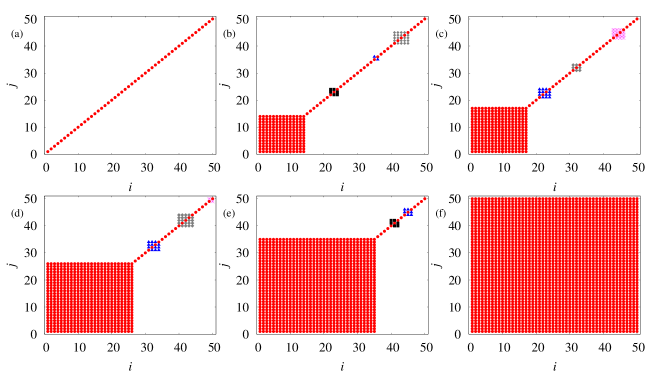
Figure 6: Oscillator index vs oscillator index snap shots indicating the sequential phase synchronization and the dynamical organization of cluster states for different values of coupling strength. The different shapes (colors) indicate that the corresponding nodes are phase synchronized. (a) non-phase synchronized case for $\varepsilon$ = 0.0 (b) First fourteen oscillators in Eq. (4b) are phase synchronized with the drive system for $\varepsilon$ = 0.45. (c), (d) and (e) Sequential phase synchronization and the formation of small cluster states for $\varepsilon$ = 0.51, 0.58 and 0.62, respectively, and (f) global phase synchronization for $\varepsilon$ = 0.8.

The nature of dynamical organization of local oscillators to form GPS can be better understood by examining the time average phase and the time average frequency as a function of the oscillator index for different values of the coupling strength. For this purpose, we define the time averaged phase ($\langle\phi_{i}\rangle$) as

$$\big{\langle}\phi_{i}(t)\big{\rangle}=\Big{\langle}2\pi k+2\pi\frac{t^{i}-t^{i}_{k}}{t^{i}_{k+1}-t^{i}_{k}}\Big{\rangle}_{t},~{}(t^{i}_{k}<t^{i}<t^{i}_{k+1}),$$ (12)

and the time averaged frequency as ($\langle\Omega_{i}\rangle$)

$$\big{\langle}\Omega_{i}(t)\big{\rangle}=\lim_{T\to\infty}\frac{1}{T}\int_{0}^{T}\dot{\phi}_{i}(t)dt,$$ (13)

where $t_{k}$ is the time of the $k^{th}$ crossing of the flow with the Poincaré section of the $i^{th}$ attractor and $\langle...\rangle_{t}$ denotes time average.

Figures 5(a) and 5(b) depict the average phase and the average frequency, respectively, for different $\varepsilon$ as a function of the oscillator index $i$. The random distribution of $\big{\langle}\phi_{i}(t)\big{\rangle}$ (Fig. 5(a)(i)) and $\big{\langle}\Omega_{i}(t)\big{\rangle}$ (Fig. 5(b)(i)) for $\varepsilon=0.0$ corresponds to the large difference in the initial frequency of the uncoupled oscillators due to the nonlinear parameter mismatch. The scenario of sequential phase synchronization to reach GPS can also be clearly visualized using the snap shots of the oscillators in the index vs index plot as shown in Fig. 6. The diagonal line in Fig. 6(a) for $\varepsilon=0.0$ clearly shows the asynchronous evolution of all the oscillators in the array.

The phase locking of the first $14$ oscillators with the drive, forming the main cluster, for $\varepsilon=0.45$ is shown in Figs. 5(a)(ii) and  5(b)(ii), while some of the other oscillators (oscillators with indices $22-24$, $35-36$ and $41-45$) away from it form phase synchronized clusters among themselves. The main cluster and other small clusters of phase synchronized oscillators are much more clearly visualized in Fig. 6(b) for the same coupling strength, in which oscillators with same frequency are assigned the same shape and color. The average phase and the average frequency for $\varepsilon=0.58$ depicted in Figs. 5(a)(iii) and Fig. 5(b)(iii) indicate that the first $26$ oscillators are synchronized with the drive with a few other small synchronized clusters away from it. Similarly, the first $35$ oscillators are synchronized with the drive for $\varepsilon=0.62$ (see Figs. 5(a)(iv) and Fig. 5(b)(iv)) along with other small clusters. Thus, it is clear that an increase in the coupling strength results in desynchronization of some of the existing clusters and formation of new clusters away from the main cluster. At the same time, nearby desynchronized oscillators from the main cluster becomes synchronized sequentially with it thereby increasing its size, contributing to the basic mechanism of formation of GPS via sequential synchronization of local oscillators as explained in detail in Ref. Suresh et al. [2010]. Finally for $\varepsilon=0.8$, all the oscillators become phase locked to attain GPS as depicted in Figs. 5(a)(v) and  5(b)(v), which remains stable for further larger values of the coupling strength. For the above values of $\varepsilon$, the main cluster and other small clusters are also clearly seen in the index vs index plot in Figs. 6.

Further, we have also plotted the average phase ($\langle\phi_{i}\rangle$) and the average frequency ($\langle\Omega_{i}\rangle$) of all the $N$ oscillators as a function of $\varepsilon$ in Figs. 7 to get a global picture of the above dynamics. Broad distribution of $\langle\phi_{i}\rangle$ and $\langle\Omega_{i}\rangle$ for small $\varepsilon$ correspond to asynchronous states while for $\varepsilon\geq 0.75$ both the average phase and average frequency converge to a single value indicating the existence of GPS. However, for the intermediate values of $\varepsilon$, the main cluster and other small clusters are hardly visible in Figs. 7. Nevertheless, these clusters are clearly seen in Figs. 5 and 6, where the snapshots of the dynamical organization of all the $N$ oscillators in the array are depicted for specific values of the coupling strength.

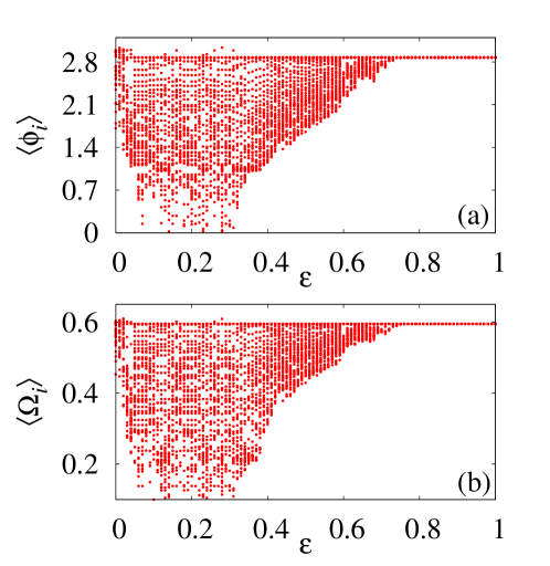
Figure 7: (a) Time averaged phase ($\langle\phi_{i}\rangle$) and (b) Time averaged frequency ($\langle\Omega_{i}\rangle$), $i=1,2,\cdots,50$ as a function of the coupling strength $\varepsilon\in(0,1.0)$. Here for each value of $\varepsilon$ we have plotted the average phase/frequency of all the $N$ = 50 oscillators which is shown by the filled circles.

The frequency difference ($\Delta\Omega_{1,i}=\Omega_{1}-\Omega_{i}$) and the frequency ratio ($\Omega_{i}/\Omega_{1}$) for the oscillators with the index $i=10,20,30,40$ and $50$ along with their average (represented by black filled circles) of all the $(N-1)$ response oscillators as a function of the $\varepsilon$ are depicted in Fig. 8(a) and Fig. 8(b), respectively. It is also clearly seen from these figures that the nearby oscillators are synchronized sequentially as $\varepsilon$ is increased, that is, $i=10$ is synchronized first and then $i=20$, and so on as $\varepsilon$ is increased. Finally, all the $N=50$ oscillators in the array are phase synchronized for $\varepsilon\geq 0.75$ attributing to the emergence of GPS via local sequential synchronization.

The well-known Kuramoto order parameter Moreno & Pacheco [2004] can also be used for quantifying the global phase synchronization in the array, which is defined as

$$R~{}e^{i\psi}=\Big{\langle}\Big{|}\frac{1}{N}\sum_{j=1}^{N}e^{i\phi_{j}(t)}\Big{|}\Big{\rangle}_{t}.$$ (14)

Here $\phi_{j}(t)$ represents the instantaneous phase of the $j^{th}$ system, $\psi(t)$ is the average phase and $\langle...\rangle_{t}$ denotes a time average. When all the systems are in a phase synchronized state, the value of $R\approx 1.0$. Figure 9 shows that $R$ decreases at first for small increase in $\varepsilon$ as observed in Figs. 8(a) and 8(b) accounting for the increased randomness in the phases of the coupled systems as seen in the average phase and the average frequency of all the oscillators in Figs. 7. Further increase in $\varepsilon$ results in a gradual increase in the value of $R$, reaching $R\approx 1.0$ for $\varepsilon>0.75$ confirming the existence of GPS in the array of coupled piecewise linear time-delay systems.

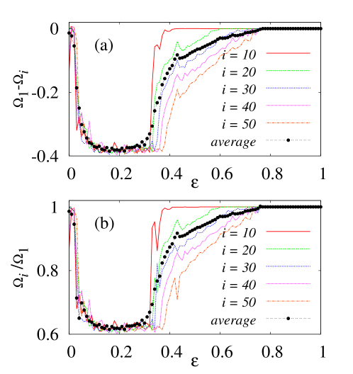
Figure 8: (a) The frequency difference ($\Delta\Omega_{1,i},\quad i=10,20,30,40$ and $50$) and (b) the frequency ratio ($\Omega_{i}/\Omega_{1},\quad i=10,20,30,40$ and $50$) of uniformly selected systems are plotted as a function of the coupling strength $\varepsilon\in(0,1.0)$. Each line corresponds to the difference/ratio between the response system and the drive system. The black filled circles indicate the average frequency difference/ratio of all the ($N-1$) response systems from the drive system.

It is also to be noted that the phenomenon remains qualitatively the same even when the total number of oscillators in the array is increased. We also wish to emphasize that the results remain qualitatively unaltered even for different sets of random values for the nonlinear parameters, $\alpha_{i}$, confirming the robustness of our results.

3.3 Confirmation of GPS from the original untransformed non-phase-coherent attractor

Next, we use two different approaches, namely recurrence quantification analysis Romano et al. [2005]; Marwan et al. [2007] and the concept of localized sets Pereira et al. [2007] without estimating the phase explicitly to prove the existence of GPS from the original nonphase coherent hyperchaotic attractors.

3.3.1 Recurrence quantification for GPS

Now, we use the recurrence quantification measures discussed in Sec. 2.2 in characterizing the existence of GPS via sequential synchronization. Figure 10 depicts the generalized autocorrelation function of the drive $P_{1}(t)$ and that of some of the response systems $P_{10}(t)$, $P_{30}(t)$, and $P_{50}(t)$ for different $\varepsilon$. For $\varepsilon=0.0$, none of the maxima of $P_{i}(t)$ coincide in Fig. 10(a) indicating asynchronous state. $P_{i}(t)$ for $i=1,10,30$ and $50$ are plotted in Figs. 10(b) and  10(c) for $\varepsilon=0.45$ and $\varepsilon=0.8$, respectively. In Fig. 10(b), the maxima of $P_{1}(t)$ and $P_{10}(t)$ are in perfect agreement (see Fig. 10(b)(i)) confirming the existence of phase synchronization

Figure 9: Plot of the phase order parameter ($R$) as a function of the coupling strength indicating global phase synchronization in the array of ($N$ = 50) coupled piecewise linear time-delay systems (4).

between the oscillators with the index $i=1$ and $i=10$, which is in agreement with the results of the earlier section. On the other hand, some of the maxima of $P_{1}(t)$ and $P_{30}(t)$ in Fig. 10(b)(ii) are in agreement attributing to the transition to CPS among them and none of the maxima of $P_{1}(t)$ and $P_{50}(t)$ in Fig. 10(b)(ii) are in agreement corresponding to independent evolution, which confirms the sequential synchronization. All the maxima of $P_{i}(t)$ are in complete agreement in Fig. 10(c) confirming the existence of GPS. Also, the formation of clusters by the other asynchronous oscillators in the array can be confirmed by plotting their respective generalized autocorrelation functions, which will show that all their maxima are in good agreement with each other, whereas there exists a drift between them and the maxima of the sequentially synchronized cluster as discussed in Ref. Suresh et al. [2010].

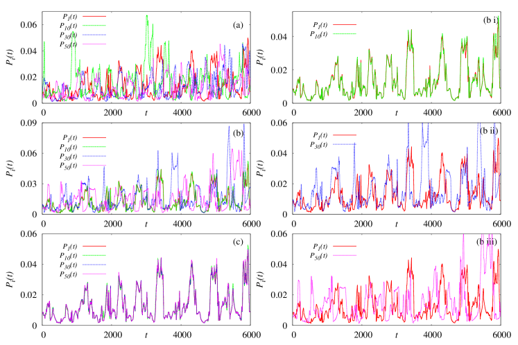
Figure 10: Plots of the Generalized autocorrelation functions of the drive $P_{1}(t)$ and some selected response systems ($i=10,30$,and, $50$) $P_{10}(t)$, $P_{30}(t)$, and $P_{50}(t)$ indicating (a) Non-phase-synchronization for $\varepsilon=0.0$, (b) generalized autocorrelation functions for $\varepsilon=0.45$ (bi) PS between the systems $1$ and $10$, (bii) approximate PS between the systems $1$ and $30$ and (biii) non PS between the systems $1$ and $50$, and (c) PS between all the systems ($i=1,10,30$, and $50$) for $\varepsilon=0.8$.

The global scenario of the existence of GPS via sequential phase synchronization can also confirmed using the index CPR in analogy with the nature of the Kuramoto order parameter $R$, the average frequency difference and the average frequency ratio. The index CPR of the response systems $i=10,20,30,50$ with that of the drive is shown in Fig. 11 as a function of $\varepsilon$. It is clear that the nearby oscillators to the drive are synchronized first as the coupling strength is gradually increased contributing to the local sequential synchronization. The results are exactly similar to that observed from the average frequency difference and the average frequency ratio in Figs. 8 indicating the phenomenon of GPS via sequential phase synchronization.

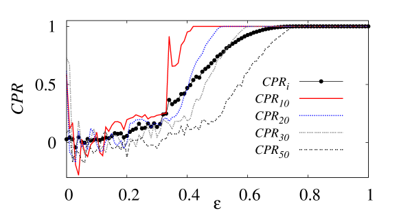
Figure 11: Plots of the index CPR as a function of the coupling strength $\varepsilon$. Different lines correspond to the CPR of different ($i=10,20,30$ and $50$) response systems with the drive system. The filled circles correspond to the mean value of the CPR of all the ($N-1$) piecewise linear systems in the array.

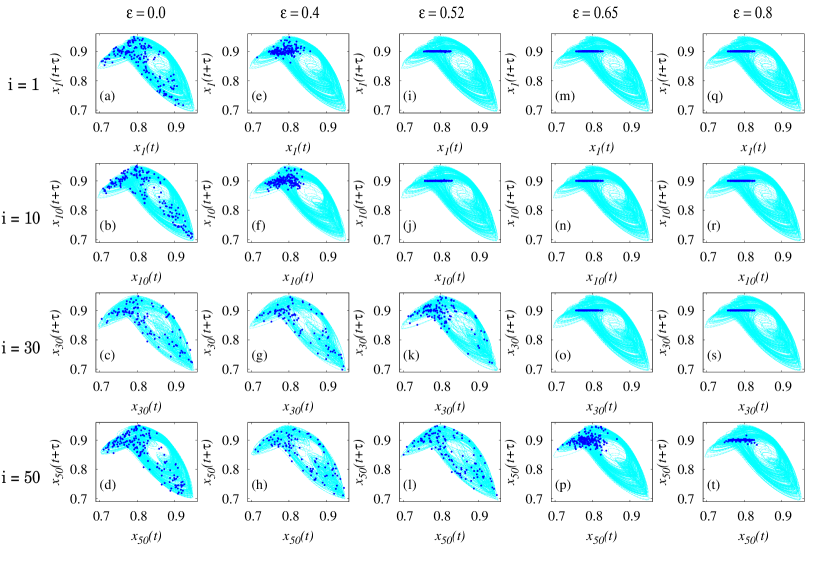
Figure 12: First row (a-q) corresponds to the attractors of the drive system ($i=1$) and the rows (b-r, c-s, and d-t) correspond to the attractors of some selected response systems ($i=10,30,50$). In (a-d) the sets (represented by the filled circles) are spread over the attractors and hence there is no CPS for the value of coupling strength $\varepsilon$ = 0.0. In (e-h) for $\varepsilon$ = 0.4 and in (i-l, m-p, q-t) the sets are localized confirming the existence of GPS in the array for $\varepsilon$ = 0.52, 0.65, and 0.8, respectively.

3.3.2 GPS using the concept of localized sets

Next, we use the framework of localized sets described in Sec. 2.3 to demonstrate the existence of GPS via sequential phase synchronization. We defined the event as a Poincaré section chosen at $x(t-\tau)=0.8$ and $x(t)<0.8$ on the attractor. The sets (indicated as filled circles) obtained by observing the drive system ($i=1$) whenever the defined event occurs in the response system $i=10$ along with the drive attractor are depicted in the first row in Fig. 12. Similarly, the sets obtained by observing the response systems ($i=10,30$ and $50$) whenever the event occurs in the drive system are depicted along with the corresponding response attractors in the other subsequent rows.

The sets spread over the entire attractors in Figs. 12(a-d) for $\varepsilon=0.0$ confirm the asynchronous evolution of the subsystems in the array. The sets localized in a large area of the attractors in Figs. 12(e-f) for $\varepsilon=0.4$ indicate the transition to CPS among the corresponding oscillators, whereas the other oscillators away from it still evolve independently as indicated by the spread of the sets over their attractors (see Figs. 12(g-h)). The more localized sets in Figs. 12(i-j) for $\varepsilon=0.52$ indicate that the respective oscillators are in complete phase synchrony while the other systems away from it are in asynchronization with it as confirmed by the spread of the sets in Figs. 12(k-l). For $\varepsilon=0.65$, the sets are bounded to smaller regions of the attractors in Figs. 12(m-o) attributing to the existence of CPS between the drive and subsystems $10$ and $30$. The other subsystem with index $i=50$ is in its transition state as indicated by the localized set but in a large region of the attractor as seen in Fig. 12(p). Thus it is clear from these figures that the oscillators away from the drive system are synchronized sequentially as the coupling strength is increased gradually. Finally, for $\varepsilon=0.8$, the sets are localized to a narrow region on the attractors (Figs. 12(q-t)) of all the subsystems thereby confirming the existence of GPS.

Figure 13: The first six maximal Lyapunov exponents $\lambda_{max}$ of the threshold piecewise linear time-delay system (Eq. (15)) for the parameter values $\alpha=1.2,\beta=1.0,\tau\in(1,10)$ in the absence of the coupling $\varepsilon$.

4 Global Phase Synchronization in an Array of Piecewise Linear Systems with Threshold Nonlinear Function

In this section, we demonstrate the existence of the GPS in another piecewise linear time-delay system with a threshold nonlinear function. This system has been studied recently for its hyperchaotic nature even for small values of time-delay [see for details, Lakshmanan & Senthilkumar, 2010] and has also been experimentally realized using analog electronic circuits Srinivasan et al. [2011]. Very recently, the chaotic phase synchronization has been experimentally confirmed in this piecewise linear time-delay system along with numerical simulation Senthilkumar et al. [2010] and various types of synchronization transitions have been demonstrated both experimentally and numerically in this system Srinivasan et al. [2011]. In this paper, we consider a linear array of piecewise linear systems as in Eq. (4) and the nonlinear function $f(x)$ is now chosen to be a piecewise linear function with a threshold nonlinearity,

$$f(x)=AF^{*}-Bx.$$ (15)

Here

$$F^{*}=\left\{\begin{array}[]{cc}-x^{*},&-x<x^{*}\\ x,&-x\leq x\leq x^{*}\\ x^{*},&x>x^{*}\\ \end{array}\right.$$ (19)

where $x^{*}$ is a controllable threshold value and $A$ and $B$ are positive parameters. This function $f(x)$ employs a threshold controller for flexibility. It effectively implements a piecewise linear function. The control of this piecewise linear function facilitates controlling the shape of the attractors. Even for a small delay value, this system exhibits hyperchaos and can produce multi-scroll chaotic attractors by just introducing more threshold values. In our analysis, we chose $x^{*}$ = 0.7, $A$ = 5.2, $B$ = 3.5, $\alpha_{1}$ = 1.2, $\beta$ = 1.0, $\tau$ = 6.0 and the nonlinear parameters $\alpha_{i}$, of the response systems in the array are chosen randomly in the range $\alpha_{i}\in(1.18,1.24)$. Note that for this set of parameter values a single uncoupled system exhibits a highly complicated hyperchaotic attractor with three positive Lyapunov exponents. The first six largest Lyapunov exponents of the uncoupled system are shown in Fig. 13 as a function of time-delay $\tau\in(1,10)$.

We have not yet succeeded in generalizing the nonlinear transformation (Eq. (1)) to capture the phase of the non-phase-coherent hyperchaotic attractor of the above systems due to the multiscroll attractor. However, we find that the recurrence-based indices serve as excellent quantifiers in identifying the transition from non-synchronized to phase synchronized state both quantitatively and qualitatively. We have also characterized the occurrence of GPS using the concept of localized sets.

4.1 GPS using recurrence analysis

We have calculated the CPR and the generalized autocorrelation function $P(t)$ to confirm the existence of the GPS in the array. The generalized autocorrelation function of the drive $P_{1}(t)$ and that of some response systems ($i=10,30$, and $50$), $P_{10}(t)$, $P_{30}(t)$, and $P_{50}(t)$, are depicted in Fig. 14 for different values of the coupling strength. In the absence of coupling ($\varepsilon=0.0$), all the systems evolve independently and hence the maxima of their respective generalized autocorrelation functions do not occur simultaneously as shown in Fig. 14(a). On increasing the coupling strength, the oscillators with a lower value of index in the array become synchronized first resulting in sequential phase synchronization and this can also be identified from the generalized autocorrelation functions of the response systems in the array. For instance, $P_{10}(t)$, $P_{30}(t)$, and $P_{50}(t)$ are shown along with $P_{1}(t)$ in Fig. 14(b) for $\varepsilon=0.8$. It is clear from this figure that the maxima of the drive $P_{1}(t)$ and those of the response $P_{10}(t)$ are in complete agreement with each other [Fig. 14(b)(i)] indicating the existence of PS between them. On the other hand, only some of the maxima of the response system $P_{30}(t)$ are in coincidence with those of the drive [Fig. 14(b)(ii)] illustrating that the response system $i=30$ is in transition to PS, whereas the maxima of the response system $P_{50}(t)$ do not coincide with those of the drive [Fig. 14(b)(iii)] indicating that the response system $i=50$ is in an asynchronous state for the same value of $\varepsilon$. For $\varepsilon=1.2$, almost all of the positions of the peaks of the generalized autocorrelation functions $P_{1}(t)$, $P_{10}(t)$, $P_{30}(t)$, and $P_{50}(t)$ are in agreement with each other as illustrated in Fig. 14(c) confirming the existence of GPS via sequential phase synchronization. It is also to be noted that the magnitudes of the peaks of all the oscillators have generally different values and these differences in the heights of the peaks indicate that there is no correlation in the amplitudes of the coupled systems.

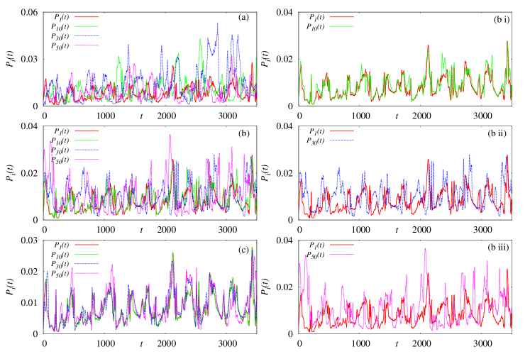
Figure 14: Generalized autocorrelation functions of the drive $P_{1}(t)$ and some of the selected response systems ($i=10,30$,and, $50$) $P_{10}(t)$, $P_{30}(t)$, and $P_{50}(t)$ indicating (a) Non-phase-synchronization for $\varepsilon=0.0$, (b) generalized autocorrelation functions for $\varepsilon=0.8$ (bi) PS between the systems $1$ and $10$, (bii) approximate PS between the systems $1$ and $30$ and (biii) non-PS between the systems $1$ and $50$, and (c) PS between all the selected systems ($i=1,10,30$, and $50$) for $\varepsilon=1.2$.

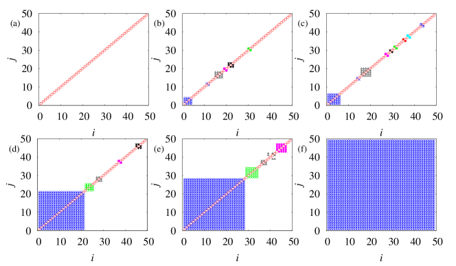
Figure 15: Snap shots of the node vs node diagrams indicating the sequential phase synchronization and the organization of cluster states for different values of coupling strength for system (4) with the threshold nonlinearity (15). (a) non-phase synchronized case for $\varepsilon$ = 0.0 (b) First four oscillators are phase synchronized with the drive system for $\varepsilon$ = 0.65. (c), (d) and (e) Sequential phase synchronization and the formation of small cluster states for $\varepsilon$ = 0.7, 0.94 and 1.13, respectively, and (f) global phase synchronization for $\varepsilon$ = 1.25.

The dynamical organization of GPS via sequential synchronization and the clustering can be visualized clearly by plotting some snap shots of the oscillators in the index vs index plots as shown in Fig. 15. The oscillators that evolve with identical phase are assigned with identical shapes (colors). The diagonal line in Fig. 15(a) for $\varepsilon=0.0$ correspond to the oscillator index $i=j$ and the oscillators evolve independently. Figure 15(b) indicates that the first four oscillators in the array are synchronized with the drive for $\varepsilon=0.65$ along with the five small separate clusters. In Fig. 15(c) for $\varepsilon=0.7$ the first six oscillators form a synchronized cluster along with eight other small clusters. Similar small clusters are shown in Fig. 15(d) and (e) for $\varepsilon=0.94$ and $\varepsilon=1.13$, respectively, in addition to the single large cluster formed by sequential phase synchronization. Finally GPS of all the systems in the array is illustrated in Fig. 15(f) for $\varepsilon=1.25$.

The existence of GPS via sequential phase synchronization is also quantified using the index CPR (2) of the response systems with the drive as shown in Fig. 16. The different lines correspond to the index of the oscillators ($i$ = 10, 20, 30, 50) in the array. It is evident from the figure that the oscillators with increasing index attain the value of unity in a sequence as a function of the coupling strength and finally for $\varepsilon>1.15$ the CPR of all the response systems with the drive reaches unity confirming that all the coupled oscillators are in GPS. The mean value of CPR of all the response systems in the array, shown as filled circles, also confirms the existence of GPS for $\varepsilon>1.15$.

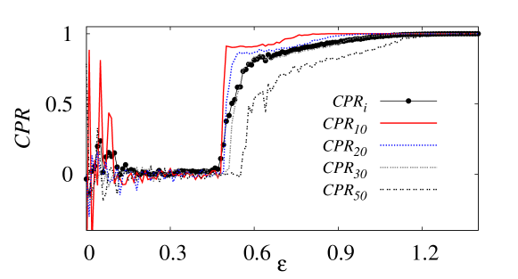
Figure 16: The index CPR as a function of the coupling strength $\varepsilon$. Different lines correspond to the CPR of different ($i=10,20,30,$ and $50$) response systems with the drive system. The filled circles correspond to the mean value of the CPR of all the ($N-1$) piecewise linear systems in the array.

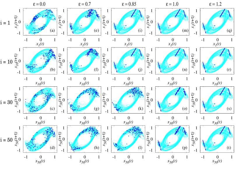
Figure 17: First row (a-q) corresponds to the attractors of the drive system ($i=1$) and the rows (b-r, c-s, and d-t) correspond to the attractors of some selected response systems ($i=10,30,50$). In (a-d) the sets (represented by the filled circles) are spread over the attractors and hence there is no CPS for the value of coupling strength $\varepsilon$ = 0.0. In (e-h) for $\varepsilon$ = 0.7 and in (i-l, m-p, q-t) the sets are localized confirming the existence of GPS in the array for $\varepsilon$ = 0.85, 1.0, and 1.2, respectively.

4.2 GPS using the concept of localized sets

We have also confirmed the existence of GPS in the linear array of threshold piecewise linear time-delay systems (Eq. (15)) by using this concept of localized sets as in the previous case. Now, we will demonstrate the existence of GPS via sequential phase synchronization in some randomly selected response systems ($i$ = 1, 10, 30, 50). The set obtained by sampling the time series of one of the systems whenever a maximum occurs in the other system is plotted along with the attractors of the same systems. The set, indicated as filled circles, obtained by observing the drive system ($i=1$) whenever the maxima occurs in the response system ($i=10$) is shown in Fig. 17(a) and that obtained by observing the response systems $i=10,30,50$ whenever the maxima occurs in the drive system are shown in Figs. 17(b-d) for the value of coupling strength $\varepsilon$ = 0.0. As the sets are spread over the attractors, all the systems evolve independently and there is no CPS in the absence of coupling between them. Further when we increase the coupling strength to $\varepsilon$ = 0.7, the oscillator ($i$ = 10) is partially synchronized with the drive as the sets are almost localized but the sets in the oscillators $i$ = 30 and 50 are spread over the attractor which means that they are not yet phase synchronized with the drive system. This is shown in Figs. 17(e-h). Again increasing the coupling strength to $\varepsilon$ = 0.85, the sets are further bounded to a small region over the attractors which shows that the oscillator $i$ = 10 is synchronized with the drive, but the oscillator $i$ = 30 is partially synchronized where the sets are almost localized and $i$ = 50 is not yet phase synchronized with the drive as represented by the spread of the sets over the attractor in Figs. 17(i-l). Further, the Figs. 17(m-p) and Figs. 17(q-t) indicate the situation for $\varepsilon$ = 1.0 and $\varepsilon$ = 1.2, respectively, where all the oscillators are now phase synchronized with the drive as the sets are localized over the attractor confirming the existence of GPS in an array via sequential phase synchronization as the coupling strength is increased. It is to be noted that the sets are not yet completely localized in Figs. 17p for $\varepsilon=1.0$, whereas it is localized for $\varepsilon=1.2$ (Figs. 17l).

Figure 18: The index CPR as a function of the system index $i$ for various values of coupling strength $\varepsilon$ in ring topology for (20). (a) For $\varepsilon=0.0$, (b) for $\varepsilon=2.22$, (c) for $\varepsilon=3.08$, (d) for $\varepsilon=3.14$, (e) for $\varepsilon=3.72$ and (f) for $\varepsilon=4.0$.

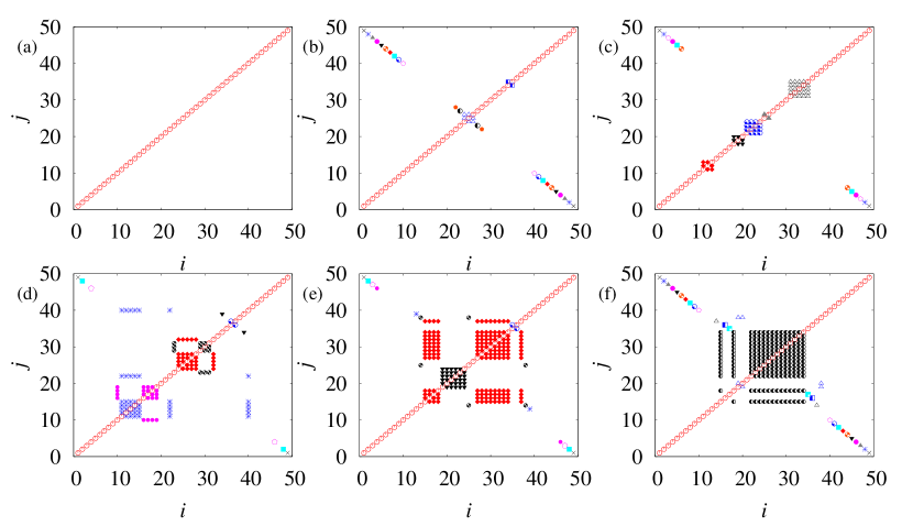
Figure 19: Snap shots of the node vs node plots for various values of coupling strengths showing the occurrence of phase clusters. (a) For $\varepsilon=0.0$, (b) for $\varepsilon=2.22$, (c) for $\varepsilon=3.08$, (d) for $\varepsilon=3.14$, (e) for $\varepsilon=3.72$ and (f) for $\varepsilon=4.0$.

5 Partial Phase Synchronization (PPS) in a Linear Array of Piecewise Linear Time-delay Systems with Ring Topology

So far we considered the dynamics of coupled arrays of time-delay systems with open end boundary conditions. Now, we wish to demonstrate the existence of a partial phase synchronization (PPS) in an array of time-delay systems with a ring topology. In this coupling configuration, all the systems are not fully synchronized, instead they split into several subgroups to form different phase synchronized clusters. The phenomenon may also be called cluster synchronization. Here the systems within each cluster maintain perfect phase synchronization. This kind of PPS mostly occurs in neural networks Denzl et al. [2008], chemical oscillations Kiss et al. [2001] and El-Ni$\tilde{n}$o systems Stein et al. [2011], and has been studied in coupled chaotic systems Bjorn et al. [2006] as well. Also the transition from nonsynchronization to phase synchronization via PPS has been studied in two-dimensional coupled map lattices Zhuang et al. [2002].

The dynamical equation of a linear array of coupled time-delay systems with closed end boundary conditions is given as

$$\dot{x}_{i}(t)=-\beta x_{i}(t)+\alpha_{i}f(x_{i}(t-\tau))+\varepsilon(x_{i-1}(t)-x_{i}(t)),$$ (20)

where $i=1,2,\cdots,N$, with the following periodic boundary conditions: $x_{0}=x_{N}$ and $x_{N+1}=x_{N}$. The function $f(x)$, and the system parameters have been chosen as in Sec. 3.1. In this type of coupling configuration the signal of the $N$th system is fed into the first system and so there is no specific drive system and that each system sends its signal to the nearby system in a unidirectional way. In the absence of the coupling, there is no synchronization among the systems. If we increase the coupling, the systems with the same phase/frequency form a small group of clusters. If we increase the coupling above a threshold value ($\varepsilon_{thr}$), PPS occurs with a relatively large group of phase clusters. For even larger values, one finds that the PPS state collapses.

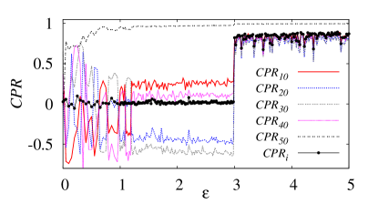
Figure 20: The index CPR as a function of the coupling strength $\varepsilon$. Different lines correspond to the CPR of different ($i=10,20,30,40$ and $50$) systems. The filled circles correspond to the mean value of the CPR of all the ($N-1$) piecewise linear systems in the array.

The nonlinear transformation used in Sec. 3 is no longer valid to transform the non-phase-coherent attractor into a phase-coherent attractor due to the new boundary condition. However, we have already found that the recurrence-based indices serve as excellent quantifiers in identifying phase synchronization in non-phase-coherent attractors both qualitatively and quantitatively. Further, we also characterized the occurrence of the cluster formation using the concept of localized sets. We will use these quantifications in the following.

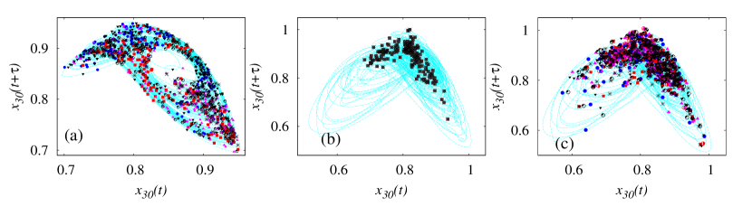
Figure 21: The occurrence of phase clusters is also explained using the concept of localized sets. (a) For $\varepsilon=0.0$ figure shows the attractor of the system $i=30$ and the sets of the systems $i=17,18,19,22$ and $31$, (randomly chosen) (b) for $\varepsilon=3.72$ with the sets of the systems inside the cluster $i=17,28,31,34$ and $37$ (which lie within the cluster). (c) for $\varepsilon=3.72$ with the sets of the systems outside the cluster $i=18,19,22$ and $27$.

We have calculated the CPR of each of the $(N-1)$ systems in the array by taking $i=1$ as the reference system (but we also confirmed that the dynamics does not change even if we take any other system in the array as a reference system). In Fig. 18 we have plotted the CPR of every system in the array as a function of the system index ($i$) for different values of coupling strength. In the absence of the coupling ($\varepsilon=0.0$), the systems in (20) evolve independently as indicated by the random distribution of CPR in Fig. 18(a). Increasing the coupling strength to $\varepsilon=2.22$ results in synchronous evolution of a few of the oscillators, leading to groups of small clusters (which are having the same CPR values) as seen in Fig. 18(b). However there is no single global synchronized state in the present network in contrast to the sequentially synchronized single cluster as discussed in Sec. 3. Above a threshold value ($\varepsilon_{thr}>3.0$), we can observe the occurrence of a PPS in the array with large groups of phase synchronized cluster. Figs. 18(c-f) indicate the occurrence of the PPS with separate groups of phase synchronized clusters for $\varepsilon=3.08$, $3.14$, $3.72$ and $4.0$, respectively. If we increase the coupling strength for even larger values, PPS continues to exist until $\varepsilon$ increases to very large values ($\varepsilon>50$) where it collapses. For very large values of the coupling strength the clusters lose their stability resulting in a desynchronized array.

Figure 22: The index CPR as a function of the system index $i$ for various values of coupling strength $\varepsilon$ in the array (20) with ring topology of the threshold piecewise linear system. (a) For $\varepsilon=0.0$, (b) for $\varepsilon=6.12$, (c) for $\varepsilon=6.80$, (d) for $\varepsilon=10.4$, (e) for $\varepsilon=11.05$, and (f) for $\varepsilon=11.8$.

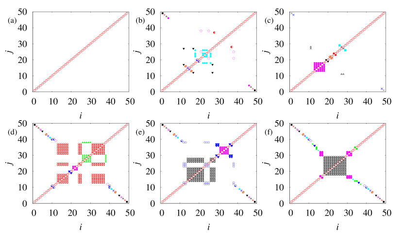
Figure 23: Snap shots of the node vs node plots for various values of coupling strengths shows the occurrence of the phase clusters in threshold piecewise linear systems. (a) For $\varepsilon=0.0$, (b) for $\varepsilon=6.12$, (c) for $\varepsilon=6.80$, (d) for $\varepsilon=10.4$, (e) for $\varepsilon=11.05$, and (f) for $\varepsilon=11.8$.

The formation of the phase synchronized clusters can also be clearly illustrated and visualized by using the snap shots of the oscillators in the index vs index plot as shown in Fig. 19. In this figure the systems with identical phase (having the difference in their CPR value less than $0.001$) are assigned with identical shapes (colors). The diagonal line in Fig. 19(a) for $\varepsilon=0.0$ correspond to the oscillator index $i=j$ and the oscillators evolve independently. Fig. 19(b) displays the occurrence of small groups of phase synchronized clusters in distant nodes ($i=2$ and $50$) for $\varepsilon=2.22$. If the coupling is increased further the nodes with the same frequency form groups of clusters with each cluster having different phases resulting in PPS. In contrast, in Fig. 6 due to the open end boundary conditions, the nearest subsystems to the drive start to synchronize with it along with the formation of small groups of clusters. Further increase in the coupling strength results in the decomposition of the small clusters which then synchronize with the main cluster. Consequently GPS results in the array with open end boundary conditions. Figs. 19(c-f) show the occurrence of PPS in the network with the formation of large phase clusters for $\varepsilon=3.08,3.14$, $3.72$ and $4.0$ respectively.

The mechanism for the formation of partial phase synchronization can be explained as follows: In the absence of the coupling the individual systems oscillate independently with different phases due to the mismatches in the nonlinear parameters $\alpha_{i}$. Upon increasing the coupling strength, due to the ring configuration, every individual oscillator starts to drive the nearest oscillator and the oscillators with small differences in their phases/frequencies in the array synchronize themselves to form small groups of clusters leaving the other oscillators with large phase differences to evolve independently. Further increase in the coupling strength results in an increase in the sizes of the clusters due to the locking of the phases of the nearby oscillators to the cluster for appropriate $\varepsilon$ and finally ending up with a large cluster near the center of the ring for large $\varepsilon$. However there exists other small clusters in the ring contributing to PPS and hence there is no GPS in such an array. As we have seen earlier in Sec. 3, in GPS, as long as the coupling increases, the nearest subsystems of the drive start to synchronize with it and the remaining asynchronous systems with the closest frequencies form small groups of phase clusters. Further increase in the coupling results in the formation of a single large cluster with the drive due to the decomposition of the small clusters with different frequencies and thereby resulting in GPS. But in the ring configuration, if the coupling increases further (above the threshold value) the distant nodes with same phase/frequency form groups of clusters with each cluster having its own phase resulting in PPS.

The synchronization transition to PPS is quantified using the value of CPR as a function of the coupling strength. In Fig. 20 the different lines correspond to the CPR of the randomly selected systems in the network ($i=10,20,30,40$ and $50$). The filled circles correspond to the mean value of the CPR of all the ($N-1$) piecewise linear systems. It is evident from this figure that only very few systems get phase synchronized to form small clusters and globally there is no phase synchronization when the coupling is below the threshold value ($\varepsilon_{thr}<3.0$) which is indicated by the mean value of CPR near to zero. Once the coupling strength crosses the threshold value ($\varepsilon\approx 3.0$), there is a sudden jump to CPR $\approx 0.8$ which is an indication of the occurrence of PPS. It is evident from this figure that the system $i=50$ is already synchronized with the drive reference system $x_{1}(t)$ as it is one of the nearest neighbors, which is also clearly seen in Figs. 18 and 19. One may note the interesting fact that this transition is of first order (sharp) type, while in the case of open end boundary condition (see Sec. 3) it is smooth and of second order type. The reason for this kind of transition is as follows: In open end boundary conditions, the subsystems are sequentially synchronized with the drive, so the GPS increases gradually in the array as a function of the coupling strength. Hence the transition is continuous (second order). But in a ring topology all the systems attain PPS suddenly at a particular value of the coupling strength due to the mutual sharing of the signals which leads to the discontinuous (first order) transition.

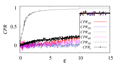
Figure 24: The index CPR as a function of the coupling strength $\varepsilon$ of the threshold piecewise linear time-delay system. Different lines correspond to the CPR of different ($i=10,20,30,40$ and $50$) systems. The filled circles correspond to the mean value of the CPR of all the ($N-1$) piecewise linear systems in the array.

Next we calculate the localized sets by defining the event among the systems within the cluster and observing the other systems that are in the same cluster. In this case the obtained sets of the systems within the cluster are localized on the attractor, while the sets of the systems outside the cluster gets spread over the entire attractor. For illustration, in Fig. 21(a) the attractor of the system $i=30$ is plotted along with the sets of the randomly selected systems $i=17,18,19,22$ and $31$ (which are represented by different shapes and colors) where the sets are spread over the attractor which corresponds to the unsynchronized state for $\varepsilon=0.0$. Fig. 21(b) corresponds to $\varepsilon=3.72$ for the sets of the systems $17,28,31,$ and $37$ which are all within the cluster. The figure shows that the sets of the corresponding systems are localized on the attractor in the same place implying that these systems form a clustered state. On the other hand, for the same value of the coupling, we have plotted the sets of the systems outside the cluster ($i=18,19,22$ and $27$). This shows that the sets are spread over the entire attractor indicating that the corresponding systems are not in phase synchronization (Fig. 21(c)).

6 Partial Phase Synchronization in an Array of Piecewise Linear Systems with Threshold Nonlinearity

In this section, we demonstrate the existence of the PPS in the second piecewise linear time-delay system with a threshold nonlinear function (15). The form of the piecewise function $f(x)$ in Eq. (20) and the system parameters are set to be the same as in Sec. 5.

In Fig. 22, the CPR is shown as a function of the system index ($i$) for different values of the coupling strength. For $\varepsilon=0.0$, in Fig. 22(a), there is no correlation in the values of CPR of the systems attributing to the desynchronization state. Figures 22(b) and 22(c) correspond to the coupling strength $\varepsilon=6.12,$ and $6.80$, respectively, which display the occurrence of small phase synchronized clusters. If we increase the coupling strength $\varepsilon>10.0$ one can observe the occurrence of PPS in the array with large groups of phase synchronized clusters. Figures 22(d-f) indicate the occurrence of the PPS with separate groups of phase synchronized clusters for $\varepsilon=10.4,11.05$ and $11.8$, respectively.

The dynamical organization of the cluster formation is clearly visualized in Fig. 23, node vs node plot, for various values of the coupling strength. The different shapes (colors) correspond to the nodes which are in the different phase synchronized clusters. In Fig. 23(a) the diagonal line shows the oscillator index $i=j$ evolving independently for $\varepsilon=0.0$. Figures 23(b) and 23(c) display the occurrence of several small phase synchronized clusters for $\varepsilon=6.12$ and $6.80$, respectively. If the coupling is increased further, the nodes with the same frequency form groups of clusters with each cluster having different phases resulting in PPS as shown in Fig. 23(d-f) for the values of $\varepsilon=10.4,11.05$ and $11.8$, respectively.

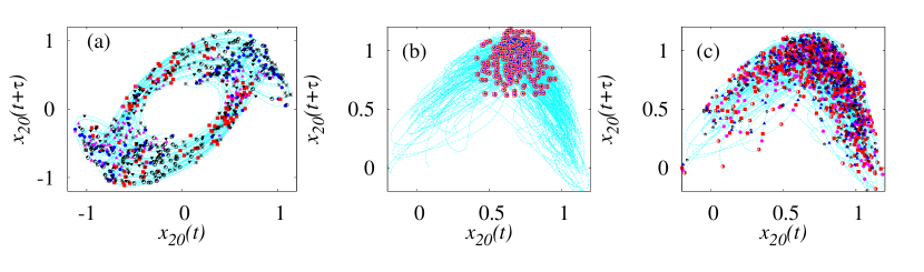
Figure 25: The occurrence of the phase clusters in threshold piecewise linear systems in the ring topology is explained using the concept of localized sets. (a) For $\varepsilon=0.0$ shows the attractor of the system $i=20$ and the sets of the systems $i=10,15,19,18,24$ and $40$, (b) for $\varepsilon=11.05$ with the sets of the systems inside the cluster $i=15,16,18$ and $26$. (c) for $\varepsilon=11.05$ with the sets of the systems outside the cluster $i=10,13,24$ and $40$.

The transition from nonsynchronization to partial phase synchronization is quantified by plotting the CPR as a function of the coupling strength. In Fig. 24 the different lines correspond to CPR of the randomly selected systems ($i=10,20,30,40$ and $50$) and the filled circles represent the mean value of the CPR of ($N-1$) systems. It is evident from this figure that there is no synchronization (CPR$<0.2$) below $\varepsilon<10.0$. There is a sudden jump (a first order transition) in the value of CPR (to $\approx 0.85$) for $\varepsilon\approx 10.0$ indicating the onset of PPS in the array along with the formation of a large group of phase synchronized clusters.

The occurrence of these phase synchronized clusters in the array of threshold piecewise linear time-delay systems is also demonstrated using the concept of localized sets. In Fig. 25, we have plotted the attractor of the system $i=20$ along with the sets of some randomly selected systems in the array. Each shapes (colors) correspond to the sets of different subsystems. Figure. 25(a) is plotted for $\varepsilon=0.0$ and the sets of the systems $i=10,15,18,24$ and $40$ spread over the entire attractor indicating the asynchronized state. For $\varepsilon=11.05$, the sets of the systems ($i=15,16,18$ and $26$) inside the large cluster are localized on the attractor as shown in Fig. 25(b) illustrating that the respective systems are in a phase synchronized state. On the other hand, for the same value of the coupling strength, we have plotted the sets of the systems outside the cluster ($i=10,13,24$ and $40$), which are spread over the attractor $i=20$ indicating that these subsystems are not in a phase synchronized state (see Fig. 25(c)).

7 Summary and Conclusion

We have demonstrated the existence of global and partial phase synchronizations in an array of unidirectionally coupled nonidentical piecewise linear time-delay systems with two different boundary conditions. Coupled with our earlier work on Mackey-Glass system Suresh et al. [2010], our studies clearly establish the generic nature of the underlying phenomena. In particular, in a linear array with open end boundary conditions, we have demonstrated the emergence of GPS via sequential synchronization. We have shown that in addition to the main phase synchronized cluster centered at the drive, the remaining asynchronous systems from the main cluster organize themselves to form different clusters for low values of the coupling strength. Further increase in the coupling strength leads to the formation of a single large cluster resulting in GPS by a decomposition of the other clusters. The synchronization transition is of second order type. We have confirmed the existence of GPS via sequential phase synchronization by estimating the phase difference, the average frequency and the average phase as a function of the oscillator index and the coupling strength from the transformed attractors. Furthermore, we have also confirmed the existence of GPS from the original non-phase-coherent attractors of the coupled piecewise linear time-delay systems using appropriate recurrence quantification measures and the concept of localized sets without explicitly estimating the phase. We have also confirmed the existence of GPS via sequential phase synchronization in a second piecewise linear system with threshold nonlinear function.

The existence of a partial phase synchronization (PPS) is demonstrated in an array with closed end boundary conditions (ring topology) and the synchronization transition is of first order type. PPS is corroborated using recurrence analysis and the concept of localized sets using the original non-phase-coherent hyperchaotic attractor of the piecewise linear time-delay systems. Further, the mechanism for the formation of both GPS and PPS are elaborated. We have also confirmed the existence of PPS in an array of Mackey-Glass time-delay systems with closed end boundary conditions; however the results are not given here as they are similar in nature to the above systems.

This study can also be extended to two-dimensional lattices of coupled time-delay systems with and without delay coupling and in networks of time-delay systems with indirect global dynamic environment coupling, as well as networks with complex topology.

References

- Amritkar & Rangarajan [2006] Amritkar, R. E. & Rangarajan, G. [2006] “Spatially synchronous extinction of species under external forcing,” Phys. Rev. Lett. 96, 258102 [4].
- Arenas et al. [2008] Arenas, A., Daz-Guilera, A., Kurths, J., Moreno, Y. & Zhou, C. [2008] “Synchronization in complex networks,” Phys. Rep. 469, 93-153.
- Bartsch et al. [2007] Bartsch, R., Kantelhardt, J. W., Penzel, T. & Havlin, S. [2007] “Experimental evidence for phase synchronization transitions in the human cardiorespiratory system,” Phys. Rev. Lett. 98, 054102 [4].
- Batista et al. [2007] Batista, C. A. S., Batista, A. M., dePontes, J. A. C., Viana, R. L. & Lopes, S. R. [2007] “Chaotic phase synchronization in scale-free networks of bursting neurons,” Phys. Rev. E 76, 016218 [10].
- Bjorn et al. [2006] Schelter, B., Winterhalder, M., Dahlhaus, R., Kurths, J. & Timmer, J., [2006] “Partial phase synchronization for multivariate synchronizing systems,” Phys. Rev. Lett. 96, 208103 [4].
- Blasius et al. [1999] Blasius, B., Huppert, A. & Stone, L. [1999] “Complex dynamics and phase synchronization in spatially extended ecological systems,” Nature (London) 399, 354-359.
- Boccaletti et al. [2002] Boccaletti, S., Kurths, J., Osipov, G., Valladares, D. L. & Zhou, C. S. [2002] “The synchronization of chaotic systems,” Phys. Rep. 366, 1-101.
- Boccaletti et al. [2006] Boccaletti, S., Latora, V., Moreno, Y., Chavez, M. & Hwang, D. U. [2006] “Complex networks: structure and dynamics,” Phys. Rep. 424, 175-308.
- Denzl et al. [2008] Danzl, P., Hansen, R., Bonnet, G. & Moehlis, J., [2008] “Partial phase synchronization of neural populations due to random Poisson imputs,” J Comput Neurosci 25, 141-157.
- Ivanchenko et al. [2004] Ivanchenko, M. V., Osipov, G. V., Shalfeev, V. D. & Kurths, J. [2004] “Phase synchronization in ensembles of bursting oscillators,” Phys. Rev. Lett. 93, 134101 [4].
- Kaneko [1990] Kaneko, K. [1990] “Clustering, coding, switching, hierarchical ordering, and control in a network of chaotic elements,” Physica D 41, 137-172.
- Kiss et al. [2001] Kiss, I. Z., Zhai, Y. & Hudson. J. L. [2002] “Collective dynamics of chaotic chemical oscillators and the law of large numbers,” Phys. Rev. Lett. 88, 238301 [4].
- Kozyreff et al. [2000] Kozyreff, G., Vladimirov, A. G. & Mandal. P. [2000] “Global coupling with time-delay in an array of semiconductor lasers,” Phys. Rev. Lett. 85, 3809-3812.
- Lakshmanan & Senthilkumar [2010] Lakshmanan, M. & Senthilkumar, D. V. [2010] Dynamics of Nonlinear Time-Delay Systems (Springer, Berlin).
- Maraun et al. [2005] Maraun, D. & Kurths, J. [2005] “Epochs of phase coherence between El Nio/southern oscillation and Indian monsoon,” Geophys. Res. Lett. 32, L15709 [5].
- Marwan et al. [2007] Marwan, N., Romano, M. C., Thiel, M. & Kurths, J, [2005] “Recurrence plots for the analysis of complex systems,” Phys. Rep. 438, 237-329.
- Moreno & Pacheco [2004] Moreno, Y. & Pacheco, A. F. [2004] “Synchronization of Kuramoto oscillators in scale-free networks,” Europhys. Lett. 68, 603-609.
- Osipov et al. [1997] Osipov, G. V., Pikovsky, A. S., Rosenblum, M. G. & Kurths, J. [1997] “Phase synchronization effects in a lattice of nonidentical Rssler oscillators,” Phys. Rev. E 55, 2353-2361.
- Osipov et al. [2007] Osipov, G. V., Zhou, C. & Kurths, J. [2007] “Synchronization in Oscillatory Networks (Springer, Berlin).
- Otsuka et al. [2006] Otsuka, K., Miyasaka, Y., Narita, T., Chu, S. C., Lin, C. C. & Ko, J. Y. [2006] “Composite lattice pattern formation in a wide-aperture thin-slice solid-state laser with imperfect reflective ends,” Phys. Rev. Lett. 97, 213901 [4].
- Pereira et al. [2007] Pereira, T., Baptista, M. S. & Kurths, J. [2007] “General framework for phase synchronization through localized sets,” Phys. Rev. E 75, 026216 [12].
- Pikovsky et al. [1996] Pikovsky, A. S., Rosenblum, M. G. & Kurths, J. [1996] “Synchronization in a population of globally coupled chaotic oscillators,” Europhys. Lett. 34, 165-170.
- Pikovsky et al. [2001] Pikovsky, A. S., Rosenblum, M. G. & Kurths, J. [2001] Synchronization - A Unified Approach to Nonlinear Science (Cambridge University Press, Cambridge, England).
- Ren & Zhao [2007] Ren, Q., Zhao, J. [2007] “Adaptive coupling and enhanced synchronization in coupled phase oscillators,” Phys. Rev. E 76, 016207 [6].
- Romano et al. [2005] Romano, M. C., Thiel, M., Kurths, J., Kiss, I. Z. & Hudson, J. L. [2005] “Detection of synchronization for non-phase-coherent and non-stationary data,” Europhys. Lett. 71, 466-472.
- Rybski et al. [2006] Rybski, D., Havlin, S. & Bunde, A. [2006] “Phase synchronization in temperature and precipitation records,” Physica A 320, 601-610.
- Schafer et al. [1998] Schfer, C., Rosenblum, M. G., Kurths, J. & Abel, H-H. [1998] “Heartbeat synchronized with ventilation,” Nature (London) 392, 239-240.
- Senthilkumar & Lakshmanan [2005] Senthilkumar, D. V. & Lakshmanan., M. [2005] “Bifurcation and Chaos in Time Delayed Piecewise Linear Dynamical Systems,” Int. J. Bifurcation and Chaos 15, 2895-2912.
- Senthilkumar & Lakshmanan [2005] Senthilkumar, D. V. & Lakshmanan., M. [2005] “Transition from anticiparoty to lag synchronization via complete synchronization in time-delay systems,” Phys. Rev. E 71, 016211 [10].
- Senthilkumar et al. [2006] Senthilkumar, D. V., Lakshmanan, M. & Kurths, J. [2006] “Phase synchronization in time-delay systems,” Phys. Rev. E 74, 035205(R)[4].
- Senthilkumar & Lakshmanan [2007] Senthilkumar, D. V. & Lakshmanan., M. [2007] “Intermittency transition to generalized synchronization in coupled time-delay systems,” Phys. Rev. E 76, 066210 [13].
- Senthilkumar et al. [2008] Senthilkumar, D. V., Lakshmanan, M. & Kurths, J. [2008] “Transition from phase to generalized synchronization in time-delay systems,” Chaos 18, 023118 [12].
- Senthilkumar et al. [2010] Senthilkumar, D. V., Srinivasan, K., Murali, K., Lakshmanan, M. & Kurths, J., [2010] “Experimental confirmation of chaotic phase synchronization in coupled time-delayed electronic circuits,” Phys. Rev. E 82, 065201(R)[4].
- Sherman [1994] Sherman, A. [1994] “Antiphase, asymmetric and aperiodic oscillations in excitable cells-I coupled bursters,” Bull. Math. Biol. 56, 811-835.
- Sismondo [1990] Sismondo, E. [1990] “Synchronous, alternating, and phase-locked stridulation by a tropical katydid,” Science 249, 55-58.
- Srinivasan et al. [2011] Srinivasan, K., Senthilkumar, D. V., Murali, K., Lakshmanan, M. & Kurths, J., [2011] “Synchronization transitions in coupled time-delay electronic circuits with a threshold nonlinearity,” Chaos 21, 023119 [11].
- Stefanovska et al. [2000] Stefanovska, A., Haken, H., McClintock, P. V. E., Hozic, M., Bajrovic, F. & Ribaric, S. [2000] “Reversable transitions between synchronization states of the cardiorespiratory system,” Phys. Rev. Lett. 85, 4831-4834.
- Stein et al. [2011] Stein, K., Timmermann, A. & Schneider, N., [2011] “Phase synchronization of the El Nino-southern oscillations with the annual cycle,” Phys. Rev. Lett. 107, 128501 [4].
- Strogatz & Stewart [1993] Strogatz, S. H. Stewart, I. [1993] “Coupled oscillators and biological synchronization,” Sci. Am. 269, 102-109.
- Suresh et al. [2010] Suresh, R., Senthilkumar, D. V., Lakshmanan, M., Kurths, J. [2010] “Global phase synchronization in an array of time-delay systems,” Phys. Rev. E 82, 016215 [10].
- Takamatsu et al. [2000] Takamatsu, A., Fujii, T. & Endo, I. [2000] “Time-delay effect in a living coupled oscillator system with the plasmodium of physarum ploycephalum,” Phys. Rev. Lett. 85, 2026-2029.
- Terry et al. [1999] Terry, J. R., Thornburg, K. S., DeShazer, Jr. D. J., VanWiggeren, G. D., Zhu, S., Ashwin, P. & Roy, R. [1999] “Synchronization of chaos in an array of three lasers,” Phys. Rev. E 59, 4036-4043.
- Yamasaki et al. [2009] Yamasaki, K., Gozolchiani, A. & Havlin, S. [2009] “Climate networks around the globe are significantely affected by El nio,” Phys. Rev. Lett. 100, 228501 [4].
- Yu et al. [2009] Yu, X., Ren, Q., Hou, J. & Zhao, J. [2009] “The chaotic phase synchronization in adaptively coupled-delayed complex networks,” Phys. Lett. A 373, 1276-1282.
- Zhan et al. [2000] Zhan, M., Zheng, Z. G., Hu, G. & Xi-hong Peng [2000] “Nonlocal chaotic phase synchronization,” Phys. Rev. E 62, 3552-3557.
- Zhou et al. [2002] Zhou, C., Kurths, J., Kiss, I. Z. & Hudson, J. L. [2002] “Noise enhanced phase synchronization of chaotic oscillators,” Phys. Rev. Lett. 89, 014101 [4].
- Zhuang et al. [2002] Zhuang, G., Wang, J., Shi, Y. & Wang, W., [2002] “Phase synchronization and its cluster feature in tow dimensional coupled map lattices,” Phys. Rev. E 66, 046201 [5].