Enhancing Bayesian risk prediction for epidemics using contact tracing

Abstract

Contact tracing data collected from disease outbreaks has received relatively little attention in the epidemic modelling literature because it is thought to be unreliable: infection sources might be wrongly attributed, or data might be missing due to resource contraints in the questionnaire exercise. Nevertheless, these data might provide a rich source of information on disease transmission rate. This paper presents novel methodology for combining contact tracing data with rate-based contact network data to improve posterior precision, and therefore predictive accuracy. We present an advancement in Bayesian inference for epidemics that assimilates these data, and is robust to partial contact tracing. Using a simulation study based on the British poultry industry, we show how the presence of contact tracing data improves posterior predictive accuracy, and can directly inform a more effective control strategy.

Keywords: Epidemic, Bayesian, reversible jump MCMC, avian influenza, contact tracing

1 Introduction

In a world in which people and animals move with increasing frequency and distance, authorities must respond to disease outbreaks at maximum efficiency according to economic, social, and political pressures. Field epidemiologists are typically faced with making decisions based on imperfect and heterogeneous data sources. European Economic Community, (1992) Council Directive 92/119/EEC requires member states to identify “other holdings…which may have become infected or contaminated”; this is achieved through contact tracing, performed by the competent authority – for instance Defra’s Framework Plan for Exotic Animal Diseases (Defra,, 2009). Though resource limitations might prevent the implementation of efficient case detection and removal based on contact tracing data (CTD), the presence of CTD might provide a rich source of information, both on contact frequency and probability of infection given a contact. In a practical setting, however, rigorous collection of contact tracing information from all detected cases is difficult to achieve; more typically, it will be collected from as many individuals as resources allow. Therefore, for a given epidemic the amount of contact tracing data available for analysis is not guaranteed in advance, the challenge for the field epidemiologist being how best to use these data to investigate disease dynamics, and inform disease control decisions.

This paper introduces a Bayesian approach to the assimilation of CTD into model-based inference and control for infectious diseases based on spatiotemporal case data. This can be applied to general classes of continuous time epidemic models, and we provide illustration using a flexible epidemic modelling framework as described in O’Neill and Roberts, (1999) and Jewell et al., 2009b ; Jewell et al., 2009a . Our methodology is particularly useful since it automatically adapts to the information contained in CTD, over and above that contained in the adjunct timeseries.

In advance of an outbreak, network and spatiotemporal dynamical models of disease have become a standard for evaluating the likely effect of various control measures, and are now routinely used for contingency planning. Using demographic data as well as case time series data, previous work has shown that real time estimation of epidemic model parameters can potentially be highly effective in informing decision-making (Cauchemez et al.,, 2006; Jewell et al., 2009a, ). In the early stages of an epidemic case data are often sparse, though this is when choosing the right course of control strategy is most critical (Anderson and May,, 1991). Therefore, decisions must often be made in the face of considerable uncertainty. For such a statistical decision support tool, assimilating different sources of data is often helpful in maximising statistical information, leading to more accurate model predictions and improved decision-making throughout the epidemic (Presanis et al.,, 2010). Nevertheless, incorporating diverse data sources into a tractable likelihood function commonly presents a methodological problem (see for example Diggle and Elliott, (1995)).

Much has been written on how contact tracing may be used to decrease the time between infection and detection (notification) during epidemics. However, this focuses on the theoretical aspects of how contact tracing efficiency is related to both epidemic dynamics and population structure. It has been shown that, providing the efficiency of following up any contacts to look for signs of disease is high, this is a highly effective method of slowing the spread of an epidemic, and finally containing it (see for example Eames and Keeling, (2003); Kiss et al., (2005); Klinkenberg et al., (2006)). In contrast, the use of CTD in inferring epidemic dynamics does not appear to have been well exploited. During the UK outbreak of foot and mouth disease in 2001, the Ministry of Agriculture, Farming, and Fisheries (now Defra) inferred a spatial risk kernel by assuming that the source of infection was correctly identified by the field investigators, giving an empirical estimate of the probability of infection as a function of distance (Ferguson et al.,, 2001; Keeling et al.,, 2001; Savill et al.,, 2006). Strikingly, this shows a high degree of similarity to spatial kernel estimates based on the statistical techniques of Diggle, (2006) and Kypraios, (2007) without using contact tracing information. However, Cauchemez et al., (2006) make the point that the analysis of imperfect CTD requires more complex statistical approaches, although they abandon contact tracing information altogether in their analysis of the 2003 SARS epidemic in China. In human health, Blum and Tran, (2010) devise a model that incorporates contact tracing for HIV-AIDS by dividing cases into those detected by random sampling or contact tracing. This allows them to estimate the proportion of undetected cases in the population at a particular observation time, although the construction of the model does not allow them to estimate the probability of infection given a contact.

Addressing this, we present a model which uses contact tracing information between pairs of individuals for time periods when it is available, and falls back on a Poisson process likelihood for time periods when it is not. We illustrate our methodology using an example from the UK agricultural industry.

In Section 2, we describe a motivating example of a potential outbreak of avian influenza in the British poultry industry. In Section 3, the existing approach to continuous time epidemic models is reviewed. Section 4 then presents our new class of embedded model for incorporating CTD. In Section 5 we develop a reversible jump Markov Chain Monte Carlo algorithm to estimate the posterior density, showing the feasibility of exact Bayesian computation for problems of this type. Section 6 then applies this methodology to the avian influenza example, showing how this methodology might be used in the event of an outbreak of high pathogenicity avian influenza.

2 Motivating Example

One motivation for this paper stems from the example of a potential avian influenza outbreak in the British poultry industry (Jewell et al., 2009a, ), using data from Defra’s Great Britain Poultry Register as well as contact network data (Dent et al.,, 2008; Sharkey et al.,, 2008). We identify three contact networks contained in the data with different levels of information. The company association network is “static”: an edge is present if and only if two poultry holding belong to the same production company. The feed mill delivery and slaughterhouse networks are “dynamic” meaning they contain edge frequency information – for example, we know not only that two holdings are connected by a feed mill delivery, but how often a feed lorry runs between them. Geographic coordinates for each holding allow us to consider non-network spatially related transmission. We also consider “background” infection sources, accounting for infections unexplained by the other transmission modes.

The presence of explicit contact networks within the poultry industry presents an interesting opportunity to investigate the possibility of including CTD into the SIR-type epidemic model (Kermack and McKendrick,, 1927). Where contact frequency data is available, we can view the networks as dynamic with contacts occurring according to a Poisson process with intensity equal to the frequency along a directed edge of the network. Normally this process is not observed, and we only have a mean contact intensity between individuals to use as covariate data in a statistical analysis. However, the collection of CTD presents the possibility for making inference from direct observations of the contact process, albeit for a select period of time leading up to a case detection.

In the typical livestock setting, CTD is gathered in response to the notification (ie case detection) of an infectious premises (IP). The resulting data are a list of contacts (with time, source, destination, and type) that have been made in and out of the IP during a period prior to the notification. The length of this period – the “contact tracing window” – during which contact tracing is gathered is stipulated by policy, and is typically longer than the expected infection to detection time for the disease in question.

Though somewhat idealised here, these data provide us a platform from which to develop the methodology required to make use of CTD for inference on epidemic models. In livestock epidemics, CTD is not routinely passed to the modelling community, and it is hoped that the results presented in this paper will encourage the authorities to do so.

3 A review of continuous time epidemic models

To begin, we provide an overview of the SINR epidemic model for heterogeneously-mixing populations (see also Jewell et al., 2009b ). The SIR model is extended by considering the population to be composed of individuals who, at any time $t$, exist in one of four states: Susceptible, Infected, Notified, and Removed. Progression through these states is assumed to be serial: individuals begin as susceptible, become infected, are notified (ie disease is detected), and are finally removed from the population (either by death, or life-long immunity). The term “individual” refers to an epidemiologically discrete unit, which might be a person or animal, or might be of higher order, such as a household or farm (as is the case for our HPAI example). It is then assumed that individuals become infected via transmission modes $k=1,\dots,K$ which might be contact network or spatial proximity to infected individuals. Independent “background” sources of infection are also included to account for infection sources other than those explicitly modelled.

Conditioning on the initial infective $\kappa$, individuals $j$ are assumed to become infected according to a time-inhomogeneous Poisson process with instantaneous rate $\lambda_{j}(t)$ equal to the sum of the infection rates across all transmission modes from all infected and notified individuals present in the population. Let $\mathcal{S}(t)$, $\mathcal{I}(t)$, $\mathcal{N}(t)$, and $\mathcal{R}(t)$ be the sets of susceptible, infected, notified, and removed individuals at time $t$, with the restriction that the entire population $\mathcal{P}=\mathcal{S}(t)\cup\mathcal{I}(t)\cup\mathcal{N}(t)\cup\mathcal{R}(t)$. Furthermore, let $\bm{I}$, $\bm{N}$, and $\bm{R}$ the corresponding vectors of individuals’ infection, notification, and removal times. Infection times are, of course, never directly observed and we therefore treat $\bm{I}$ as missing data. Since the aim of the methodology is to make inference on an epidemic in progress observed at time $T_{obs}$, infected individuals are partitioned into $j:N_{j}>T_{obs}$ occult (ie undetected) infections with right censored notification and removal times, and $j:N_{j}\leq T_{obs}$ known (ie detected) infections. Given the disease transmission parameters $\bm{\theta}=\left\{\epsilon,\bm{\beta},\gamma,\bm{p}\right\}$ (see below), the likelihood function (here denoted by $L_{A}(\cdot)$) for the epidemic process up to the analysis time $T_{obs}$ is

$$L_{A}(\bm{I},\bm{N},\bm{R}|\bm{\theta}) = \prod_{j=1,j\neq\kappa}\left(\lambda_{j}(I_{j}^{-})\right)\cdot\exp\left[-\int_{I_{\kappa}}^{T_{obs}}\left(\sum_{j\in\mathcal{P},j\neq\kappa}\lambda_{j}(t)\right)dt\right]$$ (1)

$$\times \prod_{j:N\leq T_{obs}}f_{D}\left(N_{j}-I_{j}\right)\times\prod_{j:N_{j}>T_{obs}}\left[1-F_{D}\left(T_{obs}-I_{j}\right)\right]$$

where $f_{D}(\cdot)$ is the pdf, and $F_{D}(\cdot)$ the corresponding cdf, for the infection to notification time. $\lambda_{j}(t)$ is further decomposed

$$\lambda_{j}(t)=\epsilon+\sum_{k=1}^{K}\left[\sum_{i\in\mathcal{I}(t)}\lambda_{ij}^{(k)}(t)+\gamma\sum_{i\in\mathcal{N}(t)}\lambda_{ij}^{(k)}(t)\right]$$ (2)

where $\epsilon$ represents background infection rate common to all individuals, and $\gamma$ measures the effect of quarantine measures imposed upon notified individuals. A wide range of transmission modes can then be specified, for example

$$\lambda_{ij}^{(k)}(t)=\begin{cases}q(i;\bm{\xi},t)s(j;\bm{\eta})\Psi_{k}(i,j;\psi)&\mbox{for spatial proximity}\\ q(i;\bm{\xi},t)s(j;\bm{\eta})\beta_{k}c_{ij}^{(k)}&\mbox{for \emph{associative} networks}\\ q(i;\bm{\xi},t)s(j;\bm{\eta})p_{k}r_{ij}^{(k)}&\mbox{for \emph{frequency} networks}.\end{cases}$$ (3)

In these examples, the function $0\leq q(i;\bm{\xi},t)\leq 1$ represents the infectivity of individual $i$ at time $t$, and $0\leq s(j;\bm{\eta})\leq 1$ the susceptibility of individual $j$ which is assumed constant. The rate of spatial (or environmental) transmission is given by $\Psi_{k}(i,j;\psi)$ and would typically be a function of Euclidean distance between $i$ and $j$. Network rates of transmission are represented by $\beta_{k}c_{ij}^{(k)}$ and $p_{k}r_{ij}^{(k)}$. The important distinction between the latter two terms is that $c_{ij}^{(k)}$ represents network associations (0 or 1) between $i$ and $j$ with associated infection rate $\beta_{k}$, whereas $r_{ij}^{(k)}$ represents a vector of (potentially infectious) network contact rates with associated probability $p_{k}$ that a contact results in an infection.

We remark that, if contacts are assumed to occur according to some underlying Poisson process with rate $r_{ij}^{(k)}$, infections occur according to a thinned version of this Poisson process, the thinning being governed by $p_{k}$. We assume that the contact rate is a priori independent of the probability of the infection being transmitted. Thus, a contact between infected individual $i$ and susceptible $j$ will not necessarily result in $j$ being infected, just that there is some positive probability of infection being transmitted. Considering a putative full model containing several networks, the information contained in $\bm{p}$ therefore gives a direct measure of risk for each contact network in $\bm{r}_{ij}$.

4 Incorporating Contact tracing data

Contact tracing data, $\bm{\mathcal{C}}$, represents a list of all known contacts, both incoming and outgoing, that have occurred between newly detected cases $j$ and all other individuals during a contact tracing window defined as the interval $[T_{j}^{c},N_{j})$. In other words, these data provide a means to observe the underlying contact process driving the infectious process as discussed in Section 3.

Let $C_{ijk}(t)$ be a right continuous counting process describing the number of contacts that have occurred between infected individuals $i$ and $j$ along network $k$ up to time $t$, with $\Delta C_{ijk}(t)=\lim_{\delta\downarrow 0}\left[C_{ijk}(t)-C_{ijk}(t-\delta)\right]$. If it were possible to obtain CTD for all time, as well as perfectly observing individuals’ infection states, then inference on $\bm{p}$ could be made using a geometric model with likelihood denoted by $L_{\Omega}(\cdot)$. For example

$$L_{\Omega}(\bm{I},\bm{N},\bm{R},\bm{\mathcal{C}}|\bm{p}) = \prod_{j\in\mathcal{P}}\exp\left[\int_{I_{\kappa}}^{I_{j}\wedge T_{obs}}\sum_{i\in\mathcal{Y}(t)}\sum_{k=1}^{K}Z_{ijk}(t)dC_{ijk}(t)\right]$$ (4)

$$\times \prod_{j:N\leq T_{obs}}f_{D}\left(N_{j}-I_{j}\right)\times\prod_{j:N_{j}>T_{obs}}\left[1-F_{D}\left(T_{obs}-I_{j}\right)\right]$$

with

$$Z_{ijk}(t)=\bm{1}[I_{j}=t]\log(q(i;\bm{\xi},I_{j}-I_{i})s(j;\bm{\eta})p_{k})+(1-\bm{1}[I_{j}\geq t])\log(1-q(i;\bm{\xi},I_{j}-I_{i})s(j;\bm{\eta})p_{k})$$

and $\mathcal{Y}(t)=\mathcal{I}(t)\cup\mathcal{N}(t)$.

The limitation to this approach is, of course, that CTD is only available for the contact tracing window and so the naive application of such a likelihood will give a biased estimate of $\bm{p}$.

To address this, we divide the epidemic into periods of time for which CTD is observed, and periods for which it is not. For each individual $j$ in the population, let $\mathcal{W}_{j}$ be the set of times for which contact tracing is observed (ie the contact tracing window), and $\mathcal{W}_{j}^{c}$ the set of times for which it is not. Then, the $\sigma$-algebras $\mathcal{F}=\sigma(\Delta C_{ijk}(t);t\in\mathcal{W}_{j})$ and $\mathcal{G}=\sigma(\Delta C_{ijk}(t);t\in\mathcal{W}_{j}^{c})$ represent the information contained in CTD, and that lost by not having CTD, respectively.

Theorem 1.

Where CTD is only available for contact tracing windows $\mathcal{W}_{j}$, if the underlying contact rates $r_{ij}^{(k)},k=1,\dots,K$ are known, the likelihood with respect to $\mathcal{F}$ is obtained by taking an expectation with respect to $\mathcal{G}$ such that

$$L_{\mathcal{F}}(\bm{I},\bm{N},\bm{R},\bm{\mathcal{C}}|\bm{\theta}) = \prod_{j:I_{j}\in\mathcal{W}_{j}}\exp\left[\int_{\mathcal{W}_{j}}\sum_{i\in\mathcal{Y}(t)}\sum_{k=1}^{K}Z_{ijk}(t)dC_{ijk}(t)\right]$$ (5)

$$\times \prod_{\begin{subarray}{c}j:I_{j}\in\mathcal{W}_{j}^{c}\\ j\neq\kappa\end{subarray}}\sum_{i\in\mathcal{Y}(I_{j}^{-})}\lambda_{j}(I_{j}^{-})\cdot\exp\left[-\int_{\mathcal{W}_{j}^{c}}\lambda_{j}(t)dt\right]$$

$$\times \prod_{j:N\leq T_{obs}}f_{D}\left(N_{j}-I_{j}\right)\times\prod_{j:N_{j}>T_{obs}}\left[1-F_{D}\left(T_{obs}-I_{j}\right)\right].$$

See Supplementary Material A for proof.

Theorem 1 relies on knowing the underlying contact rate for a particular network. For associative and spatial transmission modes (and indeed background pressure) the contact rate between individuals, $r_{ij}^{(k)}$, is not known and these cases do not therefore fit into our contact tracing framework. However, since the overall infection rate $\beta_{k}=p_{k}r_{ij}^{(k)}$, where it is assumed that $r_{ij}^{(k)}$ is constant with respect to both $i$ and $j$, we can regard infections via these modes as occurring due to an unobserved contact process (Equation 3). The likelihood function in Equation 5 is therefore sufficiently flexible to include these transmission modes in the $\mathcal{W}_{j}^{c}$ related terms.

Finally, we highlight that the likelihood function is written in terms of the data $\bm{I}$, $\bm{N}$, and $\bm{R}$, given the transmission parameters $\bm{\theta}$. However, the epidemic process means that infection times are never directly observed. We therefore treat $\bm{I}$ as missing data, using Bayesian data augmentation techniques described in the next section.

5 Bayesian Inference

A Bayesian approach permits the incorporation of prior information early in the epidemic, and provides a natural way to deal with $\bm{I}$, the vector of censored infection times.

Independent priors are assigned to the model parameters $\bm{\theta}=\left\{\epsilon,\bm{p},\bm{\beta},\gamma,\bm{\psi},\bm{\eta},\bm{\xi}\right\}$. Typically, Gamma distributions are used for rate parameters (ie $\epsilon$, $\bm{\beta}$, $\gamma$, $\phi$) with Beta distributions used for probability parameters (ie $\bm{p}$), as demonstrated in Section 6.

The main features of the adaptive reversible jump MCMC algorithm used to fit the model are outlined here, with full implementational details available in the Supplementary Material B. An adaptive multisite update (Haario et al.,, 2001) is used for the disease transmission parameters $\bm{\theta}$, and avoids the necessity for time consuming pilot tuning runs. This is useful to speed up the algorithm usage in a real time setting. The implementation of reversible jump (Green,, 1995) is two fold. Firstly, the dimension of $\bm{I}$ is allowed to expand or contract according to either and addition or deletion update step for occult infections from the parameter space (Jewell et al., 2009b, ). This allows the algorithm to explore the possibility occult infections present at the time of analysis consistent with the model. Secondly, infection events (including occults) are attributed to either a traced contact related to the $\mathcal{W}_{j}$ components of transmission, or spatial/untraced infections related to the $\mathcal{W}^{c}_{j}$ components. The switching in and out of the sets $\mathcal{W}_{j}$ comprises a reversible jump move, since it results in the infection appearing in different parts of the likelihood. The update step for an infection time therefore proposes the reversible jump with probability 0.5, and a contact to contact, or non-contact to non-contact move otherwise.

Shared memory parallel computing (GNU C++ using OpenMP) is used to calculate the likelihood, ensuring that the algorithm runs in an overnight timeframe (Jewell et al., 2009b, ).

6 Case study

To illustrate how this contact tracing methodology might be used in practice, we return to the dataset presented in Section 2. First we describe the special case of HPAI within the British poultry industry. Since no epidemic outbreak of HPAI has yet occurred in Britain, we provide two simulation studies to demonstrate our approach for the given model. We then demonstrate how posterior information changes in response to the amount of data available from an epidemic, both in terms of the length of the timeseries and the presence or absence of CTD. Finally we present a simulation study of 4 outbreak scenarios in which different surveillance strategies are employed for early detection of new infections.

The model

For this example, four modes of contact (Feedmill, Slaughterhouse, and Company Networks, and Spatial (environmental) transmission) contribute to the infection rate between infected or notified individual (ie farm) $i$ and susceptible $j$. For the Feedmill and Slaughterhouse networks, contact frequency information is available, whereas for the Company network only the presence or absence of a business association is known. The spatial transmission rate is then parameterised as a function of the Euclidean distance between the two individuals, centred at 5km to improve MCMC mixing and aid parameter interpretability. The transmission modes are therefore

$$\lambda_{ij}^{(1)}(t) = q(i;\bm{\xi},t)s(j;\bm{\eta})p_{1}r_{ij}^{(FM)}\bm{1}[i\in\mathcal{I}(t)]$$

$$\lambda_{ij}^{(2)}(t) = q(i;\bm{\xi},t)s(j;\bm{\eta})p_{2}r_{ij}^{(SH)}\bm{1}[i\in\mathcal{I}(t)]$$

$$\lambda_{ij}^{(3)}(t) = q(i;\bm{\xi},t)s(j;\bm{\eta})\beta_{1}c_{ij}^{(CP)}\bm{1}[i\in\mathcal{I}(t)]$$

$$\lambda_{ij}^{(4)}(t) = q(i;\bm{\xi},t)s(j;\bm{\eta})\beta_{2}e^{-\psi(\rho_{ij}-5)}$$

where $r_{ij}^{FM}$ and $r_{ij}^{SH}$ are contact frequencies for Feedmill and Slaughterhouse contacts respectively with associated probabilities of infection $p_{1}$ and $p_{2}$, $c_{ij}^{CP}$ is 0 or 1 depending on whether a business association exists between $i$ and $j$ with associated rate of infection $\beta_{1}$, $\rho_{ij}$ represents the Euclidean distance in kilometres between $i$ and $j$ with an exponential distance kernel with decay $\psi$ and parameter $\beta_{2}$ interpreted as the rate of infection between individuals 5km apart. The indicator function $\bm{1}[i\in\mathcal{I}(t)]$ removes the network transmission modes during the notified period, reflecting statutory movement restrictions on the infected farm (European Economic Community,, 1992).

The infectivity function $q(i;\bm{\xi},t)$ is defined

$$q(i;\bm{\xi},t)=\begin{cases}\frac{e^{\nu t}}{\mu+e^{\nu t}}&t\geq 0,I_{i}<t<N_{i}\\ 1&t\geq 0,N_{i}<t<R_{i}\\ 0&\mbox{otherwise}\end{cases}$$

with $\nu=1.3$ and $\mu=60$ is assumed, determined by fitting $q(i;\bm{\xi},t)$ to expert opinion. $\bm{\eta}$ is a 10-dimensional vector of susceptibilities for each production type, such that $s(j;\bm{\eta})$ returns the susceptibility of the major production species on farm $j$. In our example, we assume that broiler chickens are the most susceptible, and set this to 1. All other elements of $\bm{\eta}$ are therefore susceptibilities relative to broilers. As in our previous work, $f_{D}(\cdot)$ is given by $f_{D}(t)=ab\cdot\exp\left[bt-a\left(e^{bt}-1\right)\right]$ with $a=0.015$ and $b=0.8$ assumed, giving a mean infectious period of 6 days as determined from expert opinion. Prior distributions for the remaining parameters were chosen as suggested in Section 5, and are shown in Table 1.

Posterior information

To illustrate how the acquisition of CTD can improve posterior precision, we use a simulated epidemic on the GBPR dataset as described in Section 2, using the model described in Section 3. The epidemic is realised using a stochastic simulation based on the Doob-Gillespie algorithm (Gillespie,, 1976) applied at the level of individual contacts (to generate CTD), with the extension that retrospective sampling is used to determine whether a contact results in an infection (Jewell et al., 2009a, ).

Here we investigate how the assimilation of improves inference by increasing posterior precision. We base our test analysis on a typical simulated epidemic lasting 109 days in which 350 farms become infected, using the parameter values presented in Table 1 (see also Supplementary Material C, Figure 1). Two timepoints were analysed, day 40 (incomplete epidemic) and day 109 (complete epidemic), as shown in Table 2. CTD for a 21 day period preceeding a notification event was recorded for each notified individual. The algorithm was then run for the two timepoints during the epidemic, with and without the associated CTD.

The density plots for parameters $\epsilon$, $p_{1}$, $p_{2}$, $\beta_{1}$, $\beta_{2}$, $\gamma$, and $\psi$ are shown in Figure 1. Of particular interest are the plots for the probability parameters $p_{1}$ and $p_{2}$, which are, of course, directly informed by the contact tracing information. It is immediately apparent that the addition of contact tracing data affects the marginal posteriors of these parameters, with an increase in precision in each case. The other parameters are far less affected, with only minor differences apparent in the complete epidemic analysis. Density plots for the components of $\bm{\eta}$ and histograms of the posterior number of occults present on day 40 are shown in the Supplementary Material C, Figures 2-4.

Practical application

To test a prospective application of our methodology, we focus on the statistical detection of occult infections. We postulate that this provides a method to target limited surveillance resource to the most likely infected individuals. A simulation study was performed in which 4 surveillance strategies were tested. In the “Reactive” strategy, no active surveillance is performed, and cases are notionally detected and reported by the farmer. The 3 remaining strategies use active (pre-emptive) surveillance to look for disease as well as case detection by the farmer, with the strategy being implemented at day 14, mimicking the application of such a strategy once it has become apparent that an epidemic is taking off. “Random” surveillance represents a strategy in which a random sample of size $z$ holdings within the statutory 10km surveillance zone are visited and tested daily (Defra,, 2009). The “Bayes” targeted strategy uses our algorithm (without contact tracing data) on a daily basis to rank holdings in terms of occult probability; the top $z$ holdings are then visited and tested for disease. The “Bayes-CT” strategy then adds in CTD to target surveillance similarly. For the purposes of our simulation study, we assume a surveillance resource of $z=15$. We also assume that each surveillance team has at their disposal a perfect test for the disease - ie 100% sensitivity and specificity - and that if positive, the farm is culled immediately. For each strategy, 500 epidemic realisations with random index cases were generated to integrate over the stochasticity in the epidemic process and study the efficacy of each surveillance strategy. These were further conditioned to involve at least 2 individuals and last greater than 14 days, such that the epidemic could be said to have “taken off”. A flow diagram of the simulation study is shown in the Supplementary Material C, Figure 5.

As metrics for comparing the performance of the 4 surveillance strategies, the number of culled holdings (both as a result of Reactive and surveillance detection) and epidemic duration (ie time from the first infection to the last cull with no further infected or notified holdings) were used. These results are summarised in Table 3 and Figure 2, and indicate that active surveillance as implemented here is effective in reducing the probability of large scale outbreaks. The Random strategy, whilst successful in reducing the mean size of the outbreak, does not appreciably affect the probability of a large epidemic. Using Bayes targetting effects both of dramatically reducing the mean epidemic size and the probability of a large epidemic. The addition of CTD improves the efficacy of surveillance further: the Bayes strategy reduces the mean epidemic size by 4-fold as compared to the Reactive strategy, the Bayes-CT strategy reduces it by 10-fold. A similar picture is reflected in the results for epidemic duration, with the presence of a surveillance strategy greatly reducing the mean. As before, the effect of Bayes targeting is profound, with the presence of CTD reducing the mean variance of the duration distribution. These results suggest that Bayes targeting of surveillance using case incidence data and contact tracing may have much to offer in disease control resource prioritisation.

7 Discussion

The results presented in the previous section show contact tracing data is a useful addition for inference and prediction on SIR type epidemic models. The purpose of this methodological innovation is demonstrated well in Figure 1 showing an increase in posterior precision in response to the acquisition of the contact tracing information in parameters $p_{1}$ and $p_{2}$. Of particular interest is the behaviour of the posterior in response to differing amounts of data, and for this reason the density plots should be considered in conjunction with Table 2. For day 40, only 1 out of 4 slaughterhouse contacts resulted in infection, compared to 3 out of 28 for feedmill contacts. Importantly, the low contact frequency of the slaughterhouse network (see Supplementary Material C, Figure 6; Supplementary Material D) means that the marginal posterior for $p_{2}$ is poorly informed without the addition of contact tracing data. Conversely, the full epidemic dataset on day 109 contains more contact observations, reflected in the narrower posterior distributions. Here, there is perhaps little difference in the marginal posteriors for $p_{1}$ with and without CTD, though the effect on $p_{2}$ remains marked.

Despite its simplistic setup, the results of the surveillance strategy simulation study are encouraging, lending evidence to Bayes guided surveillance being highly effective for reducing infection to detection time, and hence abrogating the spread of an epidemic. Importantly, this methodology provides a way of immediately linking targeted surveillance to changes in outbreak dynamics due to unexpected behaviour of a new strain of the disease, changes in control strategy, or changes in underlying population behaviour – changes that may well not be apparent to the naked eye in an evolving epidemic timeseries.

Given the marked influence that CTD has on the posterior parameter estimates, care must be taken to avoid biasing the results through the use of biased datasets. The structure of the likelihood assumes independence between the data contained in individual contact tracing questionnaires (ie between individuals), and therefore the model is robust to absence of contact tracing from random cases. This is important as the analysis is unbiased in the case that the speed of the disease process exceeds the capacity to collect contact tracing data. Source of bias, however, may well arise through a case’s reluctance to declare certain contacts, and therefore carefully designing tactful contact tracing questionnaires should be of high priority. Nevertheless, in our Bayesian setup, the model extends naturally to include expert opinion on the level of such reporting bias, so an attempt to correct for it can be made.

In a UK livestock setting, although CTD is collected and used informally by field operatives to identify at risk farms, there currently appears to be no formal dissemination of this data to analysts. However, given the strong evidence for its use presented here, we strongly recommend that it should be made routinely available together with case data. Given reliable sources of such data, therefore, we envisage that real time inference and risk prediction for epidemics will become commonplace in reactive disease control strategy.

Supplementary Materials: Supplementary Material contains the proof of Theorem 1, technicalities of the rjMCMC algorithm used in Section 5, supplementary figures, and an intuition for the information gained using CTD.

Acknowledgements: We thank Professors Laura Green and Matt Keeling for helpful discussions, BBSRC for funding for this work. We thank Defra for supplying demographic data, and also for their valuable discussions on the nature of contact tracing data.

Tables and Figures

Parameter	True Value	Prior
$\epsilon$	$1^{-6}\mbox{day}^{-1}$	Gamma$(0.15,5000)$
$p_{1}$	0.3	Beta$(1,1)$
$p_{2}$	0.9	Beta$(1,1)$
$\beta_{1}$	$0.008\mbox{day}^{-1}$	Gamma$(2.048,256)$
$\beta_{2}$	$0.009\mbox{day}^{-1}$	Gamma$(2,111)$
$\gamma$	$0.5$	Gamma$(1.5,3)$
$\psi$	$0.2\mbox{km}^{-1}$	Gamma$(10,50)$
$\eta_{1}$	1	fixed
$\eta_{2}$	0.6	Gamma$(1,10)$
$\eta_{3\dots 10}$	0.3	Gamma$(1,10)$

Table 1: Transmission parameter “true” values used to simulate the test epidemic for contact tracing.

Time / days	Notified infections	Occult infections	Contacts resulting in infection		Contacts not resulting in infection
			Feedmill	S’house	Feedmill	S’house
40	159	19	3	1	25	3
109	350	0	7	5	78	12

Table 2: The state of the epidemic at each observation time. True number of epidemiologically relevant (ie originating at infectious individuals) contacts are known from the simulation algorithm.

Strategy	Mean # culled (95% CI)	Mean duration (95% CI)
SOS	203.5 (2,727)	73.2 (14.5, 147.2)
Random	120.1 (2,709)	60.0 (16.8, 122.4)
Bayes	48.1 (2,521)	23.8 (14.3, 50.5)
Bayes-CT	19.3 (2,204)	27.3 (14.2, 64.8)

Table 3: Mean number of holdings culled and mean epidemic duration (time from first infection to last removal) for each surveillance strategy, conditional on the epidemic lasting longer than 14 days. CI = credible interval.

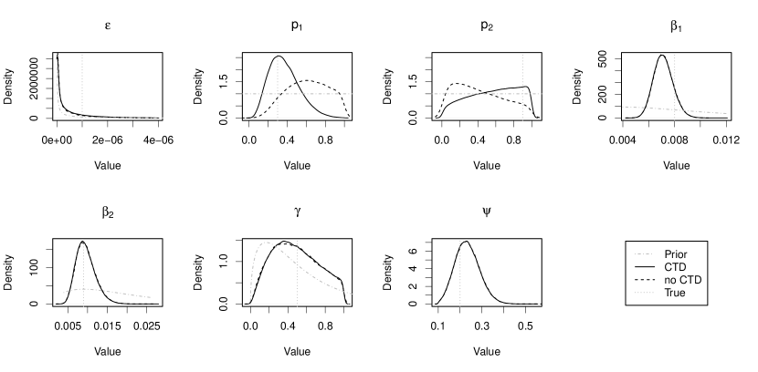
(a) Day 40

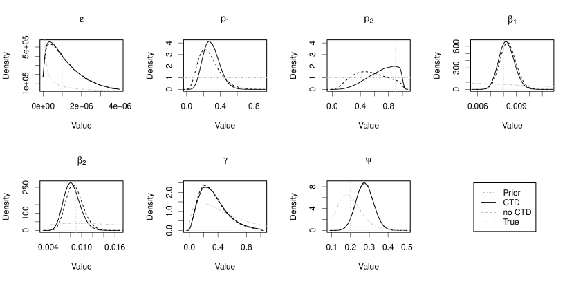
(b) Day 109

Figure 1: Kernel density estimates of the marginal posterior distributions of $\epsilon$, $p_{1}$, $p_{2}$, $\beta_{1}$, $\beta_{2}$, $\gamma$, $\psi$ for Day 40 and Day 109.

(a) The distribution of the logarithm of total number of culled premises (reactive culling plus active surveillance culls), log(mean number culled) shown by dashed lines

(b) The distribution of epidemic duration, mean duration shown by dashed lines.

Figure 2: Histograms of total number of farms culled and epidemic duration under the 4 control strategies in the simulation study.

References

- Anderson and May, (1991) Anderson, R. and May, R. (1991). Infectious diseases of humans:Dynamics and Control. Oxford University Press, New York.
- Blum and Tran, (2010) Blum, M. and Tran, V. (2010). HIV with contact tracing: a case study in approximate Bayesian computation. Biostatistics, 11:644–660.
- Cauchemez et al., (2006) Cauchemez, S., Boëlle, P.-Y., Donnelly, C., Ferguson, N., Thomas, G., Leung, G., Hedley, A., Anderson, R., and Valleron, A.-J. (2006). Real-time estimates in early detection of SARS. Emerging Infect. Dis., 12:110–113.
- Defra, (2009) Defra (2009). Contingency plan for exotic diseases of animals. [Online; Accessed 09/01/2011].
- Dent et al., (2008) Dent, J., Kao, R., Kiss, I., Hyder, K., and Arnold, M. (2008). Contact structures in the poultry industry in Great Britain: exploring transmission routes for a potential avian influenza virus epidemic. BMC Vet Res, 4:27.
- Diggle, (2006) Diggle, P. (2006). A partial likelihood for spatio-temporal point processes. Stat Methods Med Res, 15:325–36.
- Diggle and Elliott, (1995) Diggle, P. and Elliott, P. (1995). Disease risk near point sources: statistical issues for analyses using individual or spatially aggregated data. J Epidemiol Community Health, 49:S20–S27.
- Eames and Keeling, (2003) Eames, K. and Keeling, M. (2003). Contact tracing and disease control. Proc R Soc Lond B, 270:2565–2571.
- European Economic Community, (1992) European Economic Community (1992). EEC Council Directive 92/119/EEC. [Online; Accessed 09/1/2011].
- Ferguson et al., (2001) Ferguson, N., Donnelly, C., and Anderson, R. (2001). The Foot-and-Mouth Epidemic in Great Britain: Pattern of Spread and Impact of Interventions. Science, 292(5519):1155–1161.
- Gillespie, (1976) Gillespie, D. (1976). A General Method for Numerically Simulating the Stochastic Time Evolution of Coupled Chemical Reactions. Journal of Compuational Physics, 22:403–434.
- Green, (1995) Green, P. (1995). Reversible jump Markov chain Monte Carlo computation and Bayesian model determination. Biometrika, 82:711–732.
- Haario et al., (2001) Haario, H., Saksman, E., and Tamminen, J. (2001). An adaptive Metropolis algorithm. Bernoulli, 7((2)):223–242.
- (14) Jewell, C., Kypraios, T., Christley, R., and Roberts, G. (2009a). A novel approach to real-time risk prediction for emerging infectious diseases: a case study in Avian Influenza H5N1. Prev Vet Med, 91(1):19–28.
- (15) Jewell, C., Kypraios, T., Neal, P., and GO, R. (2009b). Bayesian Analysis for Emerging Infectious Diseases. Bayes. Anal., 4:465–496.
- Keeling et al., (2001) Keeling, M., Woolhouse, M., Shaw, D., Matthews, L., Chase-Topping, M., Haydon, D., Cornell, S., Kappey, J., Wilesmith, J., and Grenfell, B. (2001). Dynamics of the 2001 UK foot and mouth epidemic: Stochastic dispersal in a heterogeneous landscape. Science, 294(5543):813–818.
- Kermack and McKendrick, (1927) Kermack, W. and McKendrick, A. (1927). A Contribution to the Mathematical Theory of Epidemics. Proc. Roy. Soc. Lond. A, 115:700–721.
- Kiss et al., (2005) Kiss, I., Green, D., and Kao, R. (2005). Disease contact tracing in random and clustered networks. Proc Royal Soc B, 272:1407.
- Klinkenberg et al., (2006) Klinkenberg, D., Fraser, C., and Heesterbeek, H. (2006). The effectiveness of contact tracing in emerging epidemics. PLoS One, 1:e12.
- Kypraios, (2007) Kypraios, T. (2007). Efficient Bayesian Inference for Partially Observed Stochastic Epidemics and A New class of SemiParametric Time Series Models. PhD thesis, Department of Mathematics and Statistics, Lancaster University, Lancaster.
- O’Neill and Roberts, (1999) O’Neill, P. D. and Roberts, G. O. (1999). Bayesian inference for partially observed stochastic epidemics. J. Roy. Statist. Soc. Ser. A, 162:121–129.
- Presanis et al., (2010) Presanis, A., Gill, O., Chadborn, T., Hill, C., Hope, V., Logan, L., Rice, B., Delpech, V., Ades, A., and de Angelis, D. (2010). Insights into the rise in HIV infections in England and Wales, 2001 to 2008: a Bayesian synthesis of prevalence evidence. AIDS, 24:2849–2858.
- Savill et al., (2006) Savill, N., Shaw, D., Deardon, R., Tildesley, M., Keeling, M., Woolhouse, M., Brooks, S., and Grenfell, B. (2006). Topographic determinants of foot and mouth disease transmission in the UK 2001 epidemic. BMC Vet Res, 2:3.
- Sharkey et al., (2008) Sharkey, K., Bowers, R., Morgan, K., Robinson, S., and Christley, R. (2008). Epidemiological consequences of an incursion of highly pathogenic H5N1 avian influenza into the British poultry flock . Proc Royal Soc B, 275:19–28.