Renormalization group formalism for incompressible Euler equations and the blowup problem

Abstract

The paper discusses extensions of the renormalization group (RG) formalism for 3D incompressible Euler equations, which can be used for describing singularities developing in finite (blowup) or infinite time from smooth initial conditions of finite energy. In this theory, time evolution is substituted by the equivalent evolution for renormalized solutions governed by the RG equations. A fixed point attractor of the RG equations, if it exists, describes universal self-similar form of observable singularities. This universality provides a constructive criterion for interpreting results of numerical experiments. In this paper, renormalization schemes with multiple spatial scales are developed for the cases of power law and exponential scaling. The results are compared with the numerical simulations of a singularity in incompressible Euler equations obtained by Hou and Li (2006) and Grafke et al. (2008). The comparison supports the conjecture of a singularity developing exponentially in infinite time and described by a multiple-scale self-similar asymptotic solution predicted by the RG theory.

1 Introduction

The question of whether the incompressible Euler equations in three dimensions can develop a finite time singularity (blowup) from smooth initial conditions of finite energy is the long-standing open problem in fluid dynamics [1, 2, 3, 4]. This question is of fundamental importance, as the blowup may be related to the onset of turbulence [5] and to the energy transfer to small scales [6]. Direct numerical simulations provide a powerful tool to probe the blowup. However, despite of large effort, we are still far from having a definite answer.

There is a number of blowup and no-blowup criteria, which are useful in numerical simulations to detect a finite-time singularity. The widely used criterion is due to the Beale–Kato–Majda theorem [7], which states that the time integral of maximum vorticity must explode at a singular point. Several criteria, which also use the direction of vorticity, are developed by Constantin et al. [8], Deng et al. [9, 10] and Chae [11]. See also [1, 12, 13] and references therein.

The history of numerical studies is summarized in [3, 12, 14]. Conclusions based on numerical simulations vary depending on initial conditions and numerical method. However, none of the results seem to be sufficiently convincing so far. Apparently, the success of numerical simulations requires further development of the theory.

In this paper, we consider the renormalization group (RG) approach to the blowup problem. The RG method is famous to capture sophisticated critical phenomena characterized by scaling universality, e.g., critical phenomena in second-order phase transitions [15] and period-doubling route to chaos [16], see also the review in [17]. There are various applications of this method to problems of fluid dynamics [18]. Universality of self-similar blowup was explained in [19] for inviscid shell models of turbulence using the method, which is similar in spirit to the RG approach. Analogous universal self-similar blowup was observed in cascade models of the Euler equations [20]. The RG approach to the blowup problem for incompressible Euler equations was discussed in [21, 22, 23] in the case of a single spatial scale. In this paper, we study extension of the RG method for multiple spatial scales in the cases of power law and exponential scaling. Note that the universality predicted by the RG theory provides a constructive criterion for interpretation of numerical results.

We start by illustrating an idea of the RG method on the inviscid Burgers equation, where the blowup phenomenon is simple and well known. Here the RG equation is derived for solutions renormalized near a singularity. Fixed points of the RG equation correspond to self-similar blowup solutions. Existence of an attracting fixed point explains universal scaling of the blowup [18, 23].

The RG equations for incompressible Euler equations are derived first for the case of a single spatial scale. Fixed points of the RG equations correspond to exact self-similar solutions. A part of this theory corresponding to finite time singularities with power law scaling was considered in [21, 22, 23]. We extend the RG formalism to the case of singularities developing exponentially in infinite time. Note that exponential scaling in this problem was suggested in [24, 25] based on numerical results.

The main contribution of this paper is the development of the RG formalism with multiple spatial scales. Self-similar solutions with such scaling cannot be exact solutions of the Euler equations. However, they may serve as asymptotic solutions. This is proved by introducing a special renormalization of the pressure term in the RG equations. Attracting fixed point solutions of the RG equations, if they exist, describe universal asymptotic form of observable flow singularities. Two types of scaling are considered, which correspond to finite time (blowup) and infinite time (exponential) singularities.

The asymptotic forms of singularities provided by the RG theory are tested using the results of numerical simulations obtained by Hou and Li [26, 27] and Grafke et al. [28]. The comparison supports the conjecture of [24, 25] on exponential scaling of a singularity, which is consistent with a multiple-scale self-similar form of solution allowed by the RG theory.

The paper is organized as follows. Section 2 describes the RG theory for the inviscid Burgers equation. Section 3 describes the single-scale version of the RG formalism for the incompressible Euler equations. Section 4 develops the RG theory in the case of multiple scales. Section 5 extends the results to the case of multiple-scale exponential singularities. Section 6 compares the theory with known numerical results. Conclusion summarizes the contribution.

2 Attractor of renormalized Burgers equation

In this section we demonstrate the idea of the RG approach on a simple example of the inviscid Burgers equation

$$u_{t}+uu_{x}=0,$$ (2.1)

which has the well-known classical solution leading to a singularity in finite time (blowup). This example contains many features of the RG formalism for the incompressible Euler equations developed in the next sections.

Solution of equation (2.1) is given implicitly by the method of characteristics as

$$u(x,t)=u_{0}(z),\quad x=z+u_{0}(z)t,$$ (2.2)

where $u_{0}(x)$ is a smooth initial condition at $t=0$ and $z$ is an auxiliary variable. The blowup, $u_{x}\to\infty$, occurs when $\partial x/\partial z=0$. Expressing this derivative from the second expression in (2.2) yields $1+\partial_{z}u_{0}(z)\,t=0$. Therefore, one finds the time $t_{b}$ and position $x_{b}=z$ of the blowup from the condition

$$t_{b}=\min_{z}\left(-\frac{1}{\partial_{z}u_{0}(z)}\right).$$ (2.3)

We assume that $u_{b}=u(x_{b},t_{b})=0$ at the blowup point. This condition can always be satisfied by means of the Galilean transformation, which is a symmetry of (2.1).

Following [18], we introduce the variables

$$x^{\prime}=x-x_{b},\quad t^{\prime}=t_{b}-t,$$ (2.4)

where $t^{\prime}>0$ is the time interval to the blowup, and consider the renormalized solutions defined as

$$u(x,t)=t^{\prime(a-1)}U(\xi,\tau),\quad\xi=x^{\prime}/t^{\prime a},\quad\tau=-\log t^{\prime}.$$ (2.5)

In the new variables, the blowup corresponds to $\tau\to\infty$. Equation for $U(\xi,\tau)$ is found from (2.1), (2.5) as

$$U_{\tau}=(a-1)U-a\xi U_{\xi}-UU_{\xi}.$$ (2.6)

For $a=3/2$, this equation has a stable fixed point solution $U(\xi,\tau)=U_{*}(\xi)$ given implicitly by [18]

$$\xi=-U_{*}-CU_{*}^{3},\quad C>0.$$ (2.7)

Moreover, one can show [29] that

$$\lim_{\tau\to\infty}U(\xi,\tau)=U_{*}(\xi)$$ (2.8)

for any blowup solution with nondegenerate minimum (2.3) and some constant $C$. Note that this result extends to general scalar conservation laws [23].

Expressions (2.5) with $a=3/2$ and (2.8) imply the asymptotic relation

$$u(x,t)\to t^{\prime 1/2}U_{*}(x^{\prime}/t^{\prime 3/2}),\quad x^{\prime}\sim t^{\prime 3/2},\quad t^{\prime}\to 0.$$ (2.9)

An important observation is that this asymptotic relation is valid in the vanishingly small neighborhood $x^{\prime}\sim t^{\prime 3/2}$ of a singularity. For large $\xi=x^{\prime}/t^{\prime 3/2}$, using the approximation $U_{*}\approx-(\xi/C)^{1/3}$ following from (2.7) in (2.9) leads to the classical cubic-root expression $u(x,t)\approx-(x/C)^{1/3}$. Therefore, the wave profile $u(x,t)$ contains a universal self-similar “core” of the form (2.9) shrinking to a point as the blowup is approached. This “core” has the cubic root $x$-dependence for $x^{\prime}\gg t^{\prime 3/2}$, where it is “glued” to the rest of the solution. An example of convergence to the fixed point solution $U_{*}$ is shown in Fig. 1.

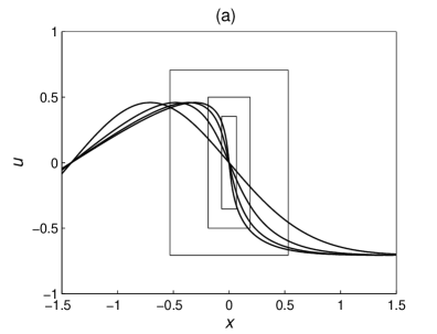
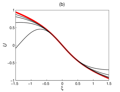
Figure 1: (a) Solution of the inviscid Burgers equation at $t^{\prime}=1$, $1/2$, $1/4$, and $1/8$, where $t^{\prime}=t_{b}-t$ is the time to blowup. Renormalization boxes, which scale as $x\sim t^{\prime 3/2}$ and $u\sim t^{\prime 1/2}$, are shown. (b) Renormalized solutions converge to the universal function $U_{*}(\xi)$, which is shown by the bold red curve.

The scaling symmetry

$$u(x,t)\mapsto b_{0}u(x/b_{0},t)$$ (2.10)

can be used to set the value $C=1$ in (2.7). The choice of $t_{b}$, $x_{b}$ at the blowup and the condition $u_{b}=0$ are important for the convergence to $U_{*}$ in (2.8), as small errors in satisfying these conditions lead to instability [18]. The values of $x_{b}$, $t_{b}$ and $u_{b}$ can always be adjusted by using the symmetry transformations

$$u(x,t)\mapsto u(x+b_{1},t),\quad u(x,t)\mapsto u(x,t+b_{2}),\quad u(x,t)\mapsto u(x+b_{3}t,t)-b_{3}.$$ (2.11)

In summary, the blowup in the inviscid Burgers equation is related to the evolution of the renormalized function $U(\xi,\tau)$ near the fixed point $U_{*}(\xi)$ in functional space demonstrated schematically in Fig. 2. The fixed point $U_{*}$ has a stable manifold $M_{S}$ of codimension 4. The four extra dimensions correspond to solutions related by symmetries (2.10) and (2.11), which determine 4-dimensional surfaces $E$ of equivalent solutions. Surfaces $E$ intersect $M_{S}$, so that one can move any point to the stable manifold by the symmetry transformation. This, in turn, implies universality of the limiting renormalized solution.

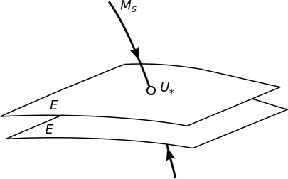
Figure 2: Schematic local structure of the fixed point $U_{*}$ of the RG equation (2.6). $M_{S}$ represents the stable manifold. Points of each surface $E$ correspond to solutions related by symmetries (2.10) and (2.11). Universal structure of the blowup is explained by the RG dynamics on the stable manifold.

One can check that the shift $\tau\mapsto\tau+\Delta\tau$ in (2.5) induces renormalization in space-time. This shift can be viewed as an action of the renormalization operator

$$U(\xi,\tau)\xrightarrow{\mathcal{R}_{\Delta\tau}}U(\xi,\tau+\Delta\tau).$$ (2.12)

Since the right-hand side of (2.6) does not depend on $\tau$ explicitly, this operator generates a one-parameter renormalization group with $\mathcal{R}_{\tau_{1}+\tau_{2}}=\mathcal{R}_{\tau_{1}}\mathcal{R}_{\tau_{2}}$. Existence of such a group is an important property underlying the above construction, similarly to other applications of the RG theory [15, 16, 17].

3 Exponential renormalization of incompressible Euler equations

The Euler equations governing the flow of ideal incompressible fluid of unit density in three dimensional space $\mathbf{x}=(x_{1},x_{2},x_{3})$ are

$$\mathbf{u}_{t}+\mathbf{u}\cdot\nabla\mathbf{u}=-\nabla p,\quad\nabla\cdot\mathbf{u}=0.$$ (3.1)

We consider solutions $\mathbf{u}(\mathbf{x},t)$ with smooth initial conditions of finite energy, $\int d^{3}x\|\mathbf{u}\|^{2}<\infty$.

First, let us assume the finite time blowup, when the flow forms a singularity at $(\mathbf{x}_{b},t_{b})$. Using the Galilean transformation, one can set $\mathbf{u}_{b}=\mathbf{u}(\mathbf{x}_{b},t_{b})=0$. Leray [30] suggested to consider self-similar solutions of the form

$$\mathbf{u}=t^{\prime(a-1)}\mathbf{U}_{*}(\mathbf{x}^{\prime}/t^{\prime a}),\quad p=t^{\prime(2a-2)}P_{*}(\mathbf{x}^{\prime}/t^{\prime a}),\quad a>0,$$ (3.2)

in the study of blowup, where

$$\mathbf{x}^{\prime}=\mathbf{x}-\mathbf{x}_{b},\quad t^{\prime}=t_{b}-t.$$ (3.3)

Finite energy solutions of this form cannot be realized globally [31, 1]. However, the global existence is not required in the RG theory, since the self-similar expression is valid asymptotically in a vanishingly small neighborhood of a singularity, see (2.9).

The renormalized solution is defined similarly to (2.5) as

$$\mathbf{u}(\mathbf{x},t)=t^{\prime(a-1)}\mathbf{U}({\bm{\xi}},\tau),\quad p(\mathbf{x},t)=t^{\prime(2a-2)}P({\bm{\xi}},\tau),\quad{\bm{\xi}}=\mathbf{x}^{\prime}/t^{\prime a},\quad\tau=-\log t^{\prime}.$$ (3.4)

Substituting these expressions into (3.1), one obtains the RG equations (see [21, 22])

$$\mathbf{U}_{\tau}=(a-1)\mathbf{U}-(a{\bm{\xi}}+\mathbf{U})\cdot\nabla_{\xi}\mathbf{U}-\nabla_{\xi}P,\quad\nabla_{\xi}\cdot\mathbf{U}=0.$$ (3.5)

A fixed point solution $\mathbf{U}_{*}({\bm{\xi}})$, $P_{*}({\bm{\xi}})$ satisfies the equations

$$(a-1)\mathbf{U}_{*}-(a{\bm{\xi}}+\mathbf{U}_{*})\cdot\nabla_{\xi}\mathbf{U}_{*}-\nabla_{\xi}P_{*}=0,\quad\nabla_{\xi}\cdot\mathbf{U}_{*}=0,$$ (3.6)

and determines the self-similar solution (3.2). The vorticity computed for the velocity (3.2) grows as ${\bm{\omega}}\sim 1/t^{\prime}$, which agrees with the Beale–Kato–Majda theorem [7].

Fixed point solutions describing the blowup are not known, but something can be said about their stability assuming that they exist [22]. Stable fixed points would describe observable blowup phenomena. Different types of attractors of the RG equations like, e.g., periodic solutions are also relevant for the blowup problem [32].

The RG formalism can be extended to the case of a singularity developing exponentially in infinite time. Assuming that the solution is regular for all $t\geq 0$ (no finite time blowup), we consider the renormalized functions $\widetilde{\mathbf{U}}({\bm{\xi}},t)$ and $\widetilde{P}({\bm{\xi}},t)$ defined as

$$\mathbf{u}(\mathbf{x},t)=e^{-bt}\widetilde{\mathbf{U}}({\bm{\xi}},t),\quad p(\mathbf{x},t)=e^{-2bt}\widetilde{P}({\bm{\xi}},t),\quad{\bm{\xi}}=\mathbf{x}^{\prime}/e^{-bt},\quad b>0.$$ (3.7)

Substituting these expressions into (3.1), one obtains the RG equations

$$\widetilde{\mathbf{U}}_{t}=b\widetilde{\mathbf{U}}-(b{\bm{\xi}}+\widetilde{\mathbf{U}})\cdot\nabla_{\xi}\widetilde{\mathbf{U}}-\nabla_{\xi}\widetilde{P},\quad\nabla_{\xi}\cdot\widetilde{\mathbf{U}}=0.$$ (3.8)

A fixed point solution $\widetilde{\mathbf{U}}_{*}({\bm{\xi}})$, $\widetilde{P}_{*}({\bm{\xi}})$ satisfies the equations

$$b\widetilde{\mathbf{U}}_{*}-(b{\bm{\xi}}+\widetilde{\mathbf{U}}_{*})\cdot\nabla_{\xi}\widetilde{\mathbf{U}}_{*}-\nabla_{\xi}\widetilde{P}_{*}=0,\quad\nabla_{\xi}\cdot\widetilde{\mathbf{U}}_{*}=0,$$ (3.9)

and determines the self-similar solution

$$\mathbf{u}(\mathbf{x},t)=e^{-bt}\widetilde{\mathbf{U}}(\mathbf{x}^{\prime}/e^{-bt}),\quad p(\mathbf{x},t)=e^{-2bt}\widetilde{P}(\mathbf{x}^{\prime}/e^{-bt})$$ (3.10)

describing a singularity developing exponentially as $t\to\infty$. Note that one can always set $b=1$ by time scaling.

The vorticity computed for the velocity (3.10) remains finite, but second spatial derivatives of the velocity grow exponentially with time. Since vorticity grows in all numerical simulations of the incompressible Euler equations, it is unlikely that stable fixed points of (3.8) exist. However, analogous exponential singularities with multiple scales described below seem to be good candidates for describing observable phenomena.

We remark that equations (3.7)–(3.10) follow from (3.2)–(3.6) in the limit $a\to\infty$. For example, the fixed point equations (3.9) are obtained from (3.6) in the limit $a\to\infty$ after multiplication by $b^{2}/a^{2}$ and the substitution $\mathbf{U}_{*}=(a/b)\widetilde{\mathbf{U}}_{*}$, $P_{*}=(a/b)^{2}\widetilde{P}_{*}$. Similar relation is established for other expressions by taking $t^{\prime}=1-b\widetilde{t}/a$ so that

$$t^{\prime a}=(1-b\widetilde{t}/a)^{a}\to e^{-b\widetilde{t}},\quad\tau=-\log t^{\prime}\to b\widetilde{t}/a$$ (3.11)

as $a\to\infty$.

Recall that, in the incompressible Euler equations, the pressure is determined by the velocity field at the same time. The same, of course, is valid for the RG equations. Indeed, computing divergence of both sides of the first expression in (3.8), the left-hand side vanishes due to the incompressibility condition and the right-hand side yields Poisson’s equation for $\widetilde{P}$. Its solution is well determined if the vector field $\widetilde{\mathbf{U}}({\bm{\xi}},t)$ decays sufficiently fast as $\|{\bm{\xi}}\|\to\infty$. However, following the results of Section 2, we can expect that the fixed point solution $\widetilde{\mathbf{U}}_{*}({\bm{\xi}})$ of the RG equations is unbounded for large $\|\bm{\xi}\|$. In this case the problem (3.9) for a fixed point is not well-posed. This inconsistency is removed in the multiple-scale RG theory considered in the next sections.

4 Multiple-scale RG formalism

Self-similar expressions of the form (3.2) or (3.10) describe singularities with a single spatial scale, $x\sim t^{\prime a}$ or $x\sim e^{-bt}$. On the other hand, numerical simulations of incompressible Euler equations available in the literature demonstrate very thin singular structures implying existence of at least two different scaling laws. For example, the two scales proposed in [33] are $x_{1}\sim 1/\sqrt{t^{\prime}}$ and $x_{2}\sim 1/t^{\prime}$. In this section, we generalize the RG formalism for the case of multiple-scale self-similar solutions.

Let us assume that solution $\mathbf{u}(\mathbf{x},t)$ with smooth initial condition of finite energy blows up in finite time at $(\mathbf{x}_{b},t_{b})$. Using the Galilean transformation, we set $\mathbf{u}_{b}=\mathbf{u}(\mathbf{x}_{b},t_{b})=0$. Let us introduce the diagonal matrices

$$t^{\prime\mathbf{A}}=\mathrm{diag}\,(t^{\prime a_{1}},t^{\prime a_{2}},t^{\prime a_{3}}),\quad\mathbf{A}=\mathrm{diag}\,(a_{1},a_{2},a_{3}),$$ (4.1)

which generalize the scaling $\mathbf{x}^{\prime}\sim t^{\prime a}$ of Section 3 to the multiple-scale case. In what follows, we assume

$$0<a_{1}\leq a_{2}<a_{3}$$ (4.2)

with a single dominant power $a_{3}$. The case of equal $a_{2}$ and $a_{3}$ can be analyzed similarly.

The renormalized solution is defined as

$$\mathbf{u}(\mathbf{x},t)=t^{\prime(\mathbf{A}-\mathbf{I})}\mathbf{U}({\bm{\xi}},\tau),\quad p(\mathbf{x},t)=t^{\prime(2a_{3}-2)}P({\bm{\xi}},\tau),\quad{\bm{\xi}}=t^{\prime-\mathbf{A}}\mathbf{x}^{\prime},\quad\tau=-\log t^{\prime},$$ (4.3)

where $\mathbf{I}$ is the identity matrix. The first relation written for each vector component has the form

$$u_{j}=t^{\prime(a_{j}-1)}U_{j}({\bm{\xi}},\tau),\quad j=1,2,3,\quad{\bm{\xi}}=(x_{1}/t^{\prime a_{1}},x_{2}/t^{\prime a_{2}},x_{3}/t^{\prime a_{3}}),$$ (4.4)

where three different scales are used for different space directions.

Substituting (4.3) into (3.1) yields

$$\mathbf{U}_{\tau}=(\mathbf{A}-\mathbf{I})\mathbf{U}-(\mathbf{A}{\bm{\xi}}+\mathbf{U})\cdot\nabla_{\xi}\mathbf{U}-\mathbf{C}\nabla_{\xi}P,\quad\nabla_{\xi}\cdot\mathbf{U}=0,$$ (4.5)

where $\mathbf{C}$ is the diagonal matrix

$$\mathbf{C}(\tau)=t^{\prime 2a_{3}}t^{\prime-2\mathbf{A}}=e^{-2a_{3}\tau}e^{2\mathbf{A}\tau}=\mathrm{diag}\,(e^{2\tau(a_{1}-a_{3})},e^{2\tau(a_{2}-a_{3})},1).$$ (4.6)

Taking time derivative of (4.6) yields the equation

$$\mathbf{C}_{\tau}=2(\mathbf{A}-a_{3}\mathbf{I})\mathbf{C}.$$ (4.7)

with the initial condition

$$\mathbf{C}(0)=\mathbf{I}.$$ (4.8)

We see that equations (4.5), (4.7) do not depend explicitly on the renormalized time $\tau$, which is the key point of the RG approach. Thus, (4.5) and (4.7) determine a renormalization group parametrized by $\tau$, as it is explained in the end of Section 2.

Let us analyze fixed points of the RG equations. According to (4.6) and (4.2), we have the constant solution

$$\mathbf{C}_{*}=\mathrm{diag}(0,0,1),$$ (4.9)

which is a fixed point attractor of (4.7) with initial condition (4.8). Then, the fixed point solution $\mathbf{U}_{*}({\bm{\xi}})$, $P_{*}({\bm{\xi}})$ of (4.5) is determined by the equations

$$(\mathbf{A}-\mathbf{I})\mathbf{U}_{*}-(\mathbf{A}{\bm{\xi}}+\mathbf{U}_{*})\cdot\nabla_{\xi}\mathbf{U}_{*}-\mathbf{C}_{*}\nabla_{\xi}P_{*}=0,\quad\nabla_{\xi}\cdot\mathbf{U}_{*}=0,$$ (4.10)

According to (4.3), the fixed point solution defines the self-similar flow

$$\mathbf{u}(\mathbf{x},t)=t^{\prime(\mathbf{A}-\mathbf{I})}\mathbf{U}_{*}(t^{\prime-\mathbf{A}}\mathbf{x}^{\prime}),\quad p(\mathbf{x},t)=t^{\prime(2a_{3}-2)}P_{*}(t^{\prime-\mathbf{A}}\mathbf{x}^{\prime}).$$ (4.11)

For each velocity component, the first expression reads

$$u_{j}(\mathbf{x},t)=t^{\prime(a_{j}-1)}U_{*j}(x^{\prime}_{1}/t^{\prime a_{1}},x^{\prime}_{2}/t^{\prime a_{2}},x^{\prime}_{3}/t^{\prime a_{3}}),\quad j=1,2,3.$$ (4.12)

Velocity field and pressure in (4.11) are not exact solutions of the Euler equations (3.1), since multiple scaling is not a symmetry of the inviscid incompressible flow. However, for solutions $\mathbf{U}$ attracted to the fixed point $\mathbf{U}_{*}$, (4.11) yields the asymptotic form of the flow. This asymptotic expression is valid in the vanishingly small neighborhood of the blowup, i.e., for

$$x^{\prime}_{1}\sim t^{\prime a_{1}},\quad x^{\prime}_{2}\sim t^{\prime a_{2}},\quad x^{\prime}_{3}\sim t^{\prime a_{3}},\quad t^{\prime}\to 0,$$ (4.13)

corresponding to constant values of ${\bm{\xi}}$. This fact can also be checked directly by substituting (4.11) into (3.1) and noting that the pressure terms of the first two Euler equations are asymptotically small. The asymptotic blowup solution (4.11) is observable, if $(\mathbf{U}_{*},P_{*},\mathbf{C}_{*})$ is an attractor of the RG equations (allowing for irrelevant unstable modes related to system symmetries, e.g., space translations and rotations).

The vorticity computed for the velocity (4.12) grows as $\omega\sim t^{\prime(a_{1}-a_{3}-1)}$ determined by the dominant derivative $\partial u_{1}/\partial x_{3}$. Since $a_{3}>a_{1}$, this agrees with the Beale–Kato–Majda theorem [7]. Note that the first two components of the vector field (4.12) satisfy exactly the Euler equations with vanishing pressure, i.e., we have

$$\partial u_{1}/\partial t+\mathbf{u}\cdot\nabla u_{1}=0,\quad\partial u_{2}/\partial t+\mathbf{u}\cdot\nabla u_{2}=0,\quad\nabla\cdot\mathbf{u}=0,$$ (4.14)

as one can check by the substitution of (4.12) into (4.14) and using (4.9), (4.10). The Euler equation for the third component remains unchanged and determines the pressure. We see that the pressure decouples from system (4.14) for the velocity components. Hence, the inconsistency related to determining the pressure function mentioned in the previous section does not appear in the multiple-scale theory.

5 Multiple-scale exponential singularity

In this section we consider extension of the multiple-scale RG theory to the case of exponential scaling introduced in Section 3. Let us assume that a flow $\mathbf{u}(\mathbf{x},t)$ with smooth initial condition of finite energy is regular for all $t\geq 0$ and forms a singularity as $t\to\infty$ at the point $\mathbf{x}_{b}$ with $\mathbf{u}_{b}=0$. Exponential renormalization with multiple scales is defined using the diagonal matrices

$$e^{\mathbf{B}t}=\mathrm{diag}\,(e^{b_{1}t},e^{b_{2}t},e^{b_{3}t}),\quad\mathbf{B}=\mathrm{diag}\,(b_{1},b_{2},b_{3}).$$ (5.1)

We consider the case

$$0<b_{1}\leq b_{2}<b_{3}$$ (5.2)

with a single dominant exponent $b_{3}$. The case of equal $b_{2}$ and $b_{3}$ can be analyzed similarly, and the single-scale solutions of Section 3 correspond to $b_{1}=b_{2}=b_{3}$.

The renormalized solution is defined as

$$\mathbf{u}(\mathbf{x},t)=e^{-\mathbf{B}t}\widetilde{\mathbf{U}}({\bm{\xi}},t),\quad p(\mathbf{x},t)=e^{-2b_{3}t}\widetilde{P}({\bm{\xi}},t),\quad{\bm{\xi}}=e^{\mathbf{B}t}\mathbf{x}^{\prime}.$$ (5.3)

The first relation written for each vector component has the form

$$u_{j}=e^{-b_{j}t}\widetilde{U}_{j}({\bm{\xi}},t),\quad j=1,2,3,\quad{\bm{\xi}}=(x_{1}/e^{-b_{1}t},x_{2}/e^{-b_{2}t},x_{3}/e^{-b_{3}t}).$$ (5.4)

Substituting (5.3) into (3.1) yields the RG equations

$$\widetilde{\mathbf{U}}_{t}=\mathbf{B}\widetilde{\mathbf{U}}-(\mathbf{B}{\bm{\xi}}+\widetilde{\mathbf{U}})\cdot\nabla_{\xi}\widetilde{\mathbf{U}}-\widetilde{\mathbf{C}}\nabla_{\xi}\widetilde{P},\quad\nabla_{\xi}\cdot\widetilde{\mathbf{U}}=0,$$ (5.5)

where $\widetilde{\mathbf{C}}$ is the diagonal matrix

$$\widetilde{\mathbf{C}}(t)=e^{-2b_{3}t}e^{2\mathbf{B}t}=\mathrm{diag}\,(e^{2t(b_{1}-b_{3})},e^{2t(b_{2}-b_{3})},1).$$ (5.6)

This matrix satisfies

$$\widetilde{\mathbf{C}}_{t}=2(\mathbf{B}-b_{3}\mathbf{I})\widetilde{\mathbf{C}},\quad\widetilde{\mathbf{C}}(0)=\mathbf{I}.$$ (5.7)

As in the previous section, we obtained the consistent RG theory, where equations (5.5), (5.7) do not depend explicitly on time. Equations (5.7) have the attracting constant solution (4.9). Thus, the fixed point solution $\widetilde{\mathbf{U}}_{*}({\bm{\xi}})$, $\widetilde{P}_{*}({\bm{\xi}})$ of (5.5) is determined by the equations

$$\mathbf{B}\widetilde{\mathbf{U}}_{*}-(\mathbf{B}{\bm{\xi}}+\widetilde{\mathbf{U}}_{*})\cdot\nabla_{\xi}\widetilde{\mathbf{U}}_{*}-\mathbf{C}_{*}\nabla_{\xi}\widetilde{P}_{*}=0,\quad\nabla_{\xi}\cdot\widetilde{\mathbf{U}}_{*}=0.$$ (5.8)

According to (5.3), the fixed point defines the self-similar asymptotic solution

$$\mathbf{u}(\mathbf{x},t)=e^{-\mathbf{B}t}\widetilde{\mathbf{U}}_{*}(e^{\mathbf{B}t}\mathbf{x}^{\prime}),\quad p(\mathbf{x},t)=e^{-2b_{3}t}\widetilde{P}_{*}(e^{\mathbf{B}t}\mathbf{x}^{\prime}).$$ (5.9)

For each velocity component, the first expression reads

$$u_{j}(\mathbf{x},t)=e^{-b_{j}t}\widetilde{U}_{*j}(x^{\prime}_{1}/e^{-b_{1}t},x^{\prime}_{2}/e^{-b_{2}t},x^{\prime}_{3}/e^{-b_{3}t}),\quad j=1,2,3.$$ (5.10)

The vorticity computed for the velocity (5.10) grows as $\omega\sim e^{(b_{3}-b_{1})t}$ determined by the dominant derivative $\partial u_{1}/\partial x_{3}$.

Similar to (4.11), velocity field and pressure in (5.9) are not exact solutions of the Euler equations (3.1), but they provide an asymptotic solution valid in the vanishingly small neighborhood of a singularity

$$x^{\prime}_{1}\sim e^{-b_{1}t},\quad x^{\prime}_{2}\sim e^{-b_{2}t},\quad x^{\prime}_{3}\sim e^{-b_{3}t},\quad t\to\infty.$$ (5.11)

This solution describes an observable singularity, if the fixed point $(\widetilde{\mathbf{U}}_{*},\widetilde{P}_{*},\mathbf{C}_{*})$ is an attractor of the RG equations (allowing for irrelevant unstable modes related to system symmetries). In this case, (5.10) is a universal asymptotic form of a singularity. Note that the coefficients $b_{1}$, $b_{2}$ and $b_{3}$ are multiplied by the same positive factor under a change of time scale and, hence, only the ratios $b_{1}/b_{3}$ and $b_{2}/b_{3}$ are expected to be universal. As in Section 3, one can obtain the multiple-scale exponential singularity expressions as the limit of the formulas for blowup in Section 4 with $a_{j}=b_{j}a$ and $a\to\infty$. Also, the asymptotic solution (5.9) is the exact solution of (4.14), as it can be checked by the substitution using (5.8).

We remark that a scaling of pressure different from (4.3) and (5.3) can also be considered in the RG scheme. For example, the scaling $p(\mathbf{x},t)=\widetilde{P}({\bm{\xi}},t)$ with $b_{1}=b_{2}=1$ was suggested in [25]. For such scaling, however, the problem for fixed points of the RG equations is not well-posed, due to similar reasons as described in Section 3.

6 Self-similar exponential singularity in numerical simulations

In several studies, numerical solutions were interpreted in favor of finite-time blowup, suggesting the growth of maximum vorticity as $\max|\omega|\sim 1/t^{\prime}$, see, e.g., [34, 35]. However, this asymptotic relation was not confirmed in later computations [36, 28]. Several numerical studies [25, 37, 28] suggested exponential time dependence of vorticity. Self-similarity of numerical solutions was discussed in [24, 25, 33]. See also the review of numerical results in [3].

Fig. 3 shows dependence of maximum vorticity on time reconstructed from Fig. 9 in [27] and Fig. 1 in [28]. Initial conditions in these simulations have the form of antiparallel vortex tubes in [27] and of Kide–Pelz 12 vortices in [28]. Logarithmic scale is used for the maximum vorticity. One can see that $\max|\omega|$ is approximated very well by the exponential time dependence (straight dashed lines) for large times. Similar exponential behavior was observed along a Lagrangian trajectory passing near the singularity, see Fig. 5 in [28].

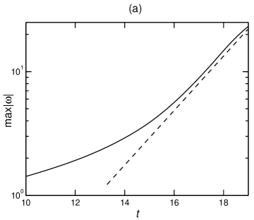
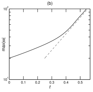
Figure 3: Dependence of the maximum vorticity in log-scale on time reconstructed from (a) Fig. 9 in [27] and (b) Fig. 1 in [28]. One can notice the asymptotic exponential time dependence (straight dashed lines).

In this section, we use the RG formalism to test the conjecture [25] on exponential scaling and self-similarity of flow near a singularity. The appropriate self-similar solution is described by (5.10). For maximum vorticity, it yields the asymptotic relation $\max|\omega|\approx\omega_{0}e^{(b_{3}-b_{1})t}$ given by the dominant term $\partial u_{1}/\partial x_{3}$, in agreement with Fig. 3.

It is convenient to use the Fourier transformed form of (5.10) as

$$u_{j}(\mathbf{k},t)=e^{-(b_{j}+b_{1}+b_{2}+b_{3})t}\widetilde{U}_{*j}(k_{1}/e^{b_{1}t},k_{2}/e^{b_{2}t},k_{3}/e^{b_{3}t}),\quad j=1,2,3,$$ (6.1)

where $\mathbf{u}(\mathbf{k},t)$ is the Fourier transform of $\mathbf{u}(\mathbf{x}_{b}+\mathbf{x}^{\prime},t)$ and $\widetilde{\mathbf{U}}_{*}(\mathbf{k})$ is the Fourier transform of $\widetilde{\mathbf{U}}_{*}({\bm{\xi}})$. The asymptotic relation (5.10) is valid in a small neighborhood of a singularity in physical space (5.11). Hence, the self-similarity must be observed for large $k_{j}$, namely, for

$$k_{j}\sim e^{b_{j}t},\quad j=1,2,3,\quad t\to\infty.$$ (6.2)

In particular, it follows from (6.2) with the conditions (5.2) that, for large $t$,

$$k_{1}\ll k_{3},\quad k_{2}\ll k_{3},\quad k=\|\mathbf{k}\|\approx k_{3}.$$ (6.3)

This means that the self-similar part of solution is concentrated near the axis $k_{3}$ in the Fourier space. Expressions (6.1)–(6.3) imply the self-similar asymptotic behavior of the energy spectrum

$$E(k,t)\approx e^{-b_{E}t}\widetilde{E}(k/e^{b_{3}t}),\quad k\approx k_{3}\sim e^{b_{3}t},\quad t\to\infty,$$ (6.4)

which scales as the dominant variable $k_{3}$. The function $\widetilde{E}(k)$ and the constant $b_{E}$ can be expressed in terms of $\widetilde{\mathbf{U}}_{*}(\mathbf{k})$ and $b_{j}$.

Below we verify the self-similarity hypothesis by checking (6.4) for the numerical data reconstructed from Figs. 9 and 10 in [26]. Fig. 4(a) shows the graphs of energy spectra $E(k,t)$ at times $t=15,16,17$ before and after the scaling chosen as

$$E(k,15),\quad e^{1.5}E(e^{0.43}k,16),\quad e^{3}E(e^{0.93}k,17).$$ (6.5)

Good matching of the scaled profiles is observed. The scaling exponents change almost linearly in time in agreement with the asymptotic expression (6.4). Similar behavior was observed in [24, 25] based on the approximation $E(k,t)=c(t)k^{-n(t)}e^{-2\delta(t)k}$.

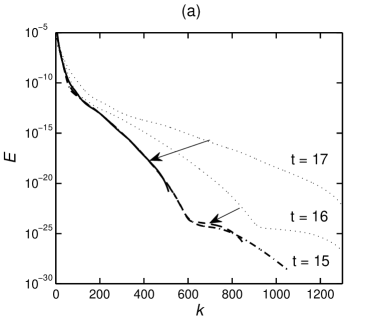
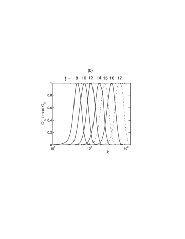
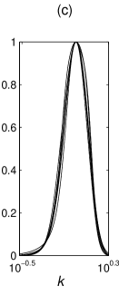
Figure 4: Energy spectra reconstructed from Figs. 9 and 10 in [26]. (a) Energy spectra before and after scaling (6.5). Log-scale is used for $E$. The scaled spectra match in agreement with (6.4). (b) Normalized spectra $\Omega_{6}(k,t)$ at different times with log-scale for $k$ demonstrating a “traveling wave” moving toward large $k$. (c) Profiles of the previous figure shifted to match at the maximum, demonstrating self-similar asymptotic form in agreement with (6.6).

More detailed analysis can be carried out using the spectra $\Omega_{n}(k,t)=k^{2n}E(k,t)$ of generalized enstrophies considered earlier in [24]. According to (6.4), these spectra must scale exponentially in time as

$$\Omega_{n}(k,t)\approx e^{(2nb_{3}-b_{E})t}\widetilde{\Omega}_{n}(k/e^{b_{3}t}),\quad k\sim e^{b_{3}t},\quad t\to\infty,$$ (6.6)

where $\widetilde{\Omega}_{n}(k)=k^{2n}\widetilde{E}(k)$. The reason to consider $\Omega_{n}(k,t)$ instead of $E(k,t)$ is the following. For sufficiently large $n$, the factor $k^{2n}$ (corresponding to the spatial mean-square derivative) suppresses the energy spectrum in the region of small wave numbers, $k\ll e^{b_{3}t}$, where the asymptotic relation (6.6) is not valid. As a result, the function $\Omega_{n}(k,t)$ is large for $k\sim e^{b_{3}t}$, where the self-similarity is expected, and gets small far from this region.

Fig. 4(b) shows the function $\Omega_{6}(k,t)$ divided by its maximum value at times $t=8$, $10$, $12$, $14$, $15$, $16$, $17$. The shape of this function is almost independent of time, as shown in Fig. 4(c), where the profiles are shifted to match at the maximum. Fig. 5 presents the values of $\displaystyle\max_{k}\Omega_{6}$ and the corresponding values of $k$ for the profiles in Fig. 4(b). The plots demonstrate asymptotic exponential dependence for $t\geq 14$ (straight dashed lines in logarithmic scale). Fig. 5 can be compared with the asymptotic exponential growth of maximum vorticity in Fig. 3(a), corresponding to the same numerical simulation. Note that the blowup in the inviscid Burgers equation (2.1) as well as in inviscid shell models of turbulence is characterized in the Fourier space by the behavior very similar to Fig. 4(b) under appropriate renormalization, see [19, 23].

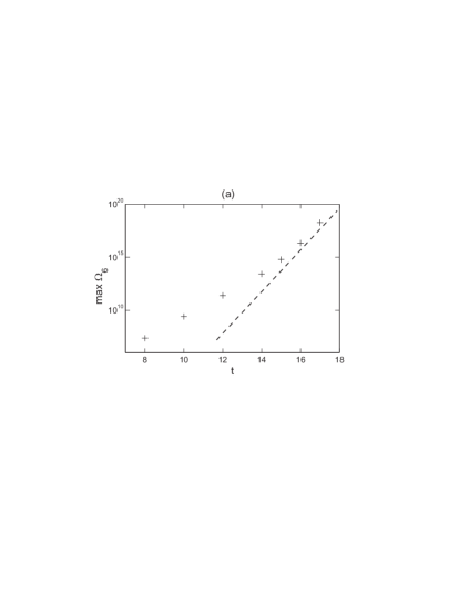
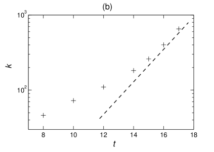
Figure 5: Analysis of energy spectra reconstructed from Figs. 9 and 10 in [26]. Shown are the time dependence of (a) $\displaystyle\max_{k}\Omega_{6}(k,t)$ and (b) the corresponding values of $k$ for the profiles in Fig. 4(b). Log-scale is used for the vertical coordinate, demonstrating asymptotic exponential dependence (dashed lines).

The presented analysis of numerical results supports the conjecture that the inviscid incompressible flow has a singularity developing exponentially in time and having asymptotic self-similar structure (5.10). The RG theory of Section 5 suggests that the renormalized velocity field and ratios of scaling coefficients may be universal, i.e., independent of initial conditions. This universality is a powerful criterion, which can be checked numerically. Such a test, however, is nontrivial, since the universality may be sensitive to symmetry transformations, see Section 2.

7 Conclusion

The problem of existence and structure of singularities developing in finite time (blowup) or infinite time from smooth initial conditions of finite energy in incompressible Euler equations is considered. These singularities may be studied using the renormalization group (RG) approach. The central point of this approach is deriving the RG equations, which determine the flow evolution combined with renormalization of space, time and velocities. A fixed point attractor of the RG equations, if it exists, describes a universal self-similar form of observable singularities.

In this paper, we described extensions of the RG formalism, which include multiple scales and different scaling laws. We explained the possibility of two types of universal self-similar flow structures valid asymptotically in a small neighborhood of a singularity. The first type describes formation of a finite time singularity (blowup) with the power law scaling $x^{\prime}_{j}\sim t^{\prime a_{j}}$, $j=1,2,3$. In the limit $a_{j}\to\infty$, we obtain the second type corresponding to solutions with exponential scaling, $x^{\prime}_{j}\sim e^{-b_{j}t}$, which describe singularities developing exponentially in infinite time. Such a limit implies, in particular, that the exponential (infinite time) singularity cannot be distinguished by numerical methods from the finite-time blowup with very large scaling coefficients $a_{j}$.

We showed that numerical results obtained by Hou and Li [26, 27] and Grafke et al. [28] support the conjecture of exponential scaling of flow singularity [24, 25]. The analysis shows that the singularity may be described by a universal self-similar solution given by the RG theory. The universality provides an effective criterion to be considered in future numerical studies. One should take into account, however, that universality may be sensitive to system symmetries.

References

- [1] D. Chae. Incompressible Euler Equations: the blow-up problem and related results. In: Handbook of Differential Equations: Evolutionary Equations (C.M. Dafermos and M. Pokorny, Eds.), Vol. 4, pages 1–55. Elsevier, 2008.
- [2] P. Constantin. On the Euler equations of incompressible fluids. B. Am. Math. Soc., 44(4):603–622, 2007.
- [3] J.D. Gibbon. The three-dimensional Euler equations: Where do we stand? Phys. D, 237(14-17):1894–1904, 2008.
- [4] J.D. Gibbon, M. Bustamante, and R.M. Kerr. The three-dimensional Euler equations: singular or non-singular? Nonlinearity, 21:T123, 2008.
- [5] D.D. Holm and R. Kerr. Transient vortex events in the initial value problem for turbulence. Phys. Rev. Lett., 88(24):244501, 2002.
- [6] G.L. Eyink and K.R. Sreenivasan. Onsager and the theory of hydrodynamic turbulence. Rev. Modern Phys., 78(1):87–135, 2006.
- [7] J.T. Beale, T. Kato, and A. Majda. Remarks on the breakdown of smooth solutions for the 3-D Euler equations. Comm. Math. Phys., 94(1):61–66, 1984.
- [8] P. Constantin, C. Fefferman, and A.J. Majda. Geometric constraints on potentially singular solutions for the 3-D Euler equations. Comm. Partial Differential Equations, 21(3-4):559–571, 1996.
- [9] J. Deng, T. Hou, and X. Yu. Improved geometric conditions for non-blowup of the 3D incompressible Euler equation. Comm. Partial Differential Equations, 31(2):293–306, 2006.
- [10] J. Deng, Y.H. Thomas, and X. Yu. Geometric properties and nonblowup of 3D incompressible Euler flow. Comm. Partial Differential Equations, 30(1-2):225–243, 2005.
- [11] D. Chae. On the finite-time singularities of the 3D incompressible Euler equations. Comm. Pure Appl. Math., 60(4):597–617, 2007.
- [12] T.Y. Hou. Blow-up or no blow-up? A unified computational and analytic approach to 3D incompressible Euler and Navier–Stokes equations. Acta Numer., 18(1):277–346, 2009.
- [13] E.A. Kuznetsov. Towards a sufficient criterion for collapse in 3D Euler equations. Phys. D, 184(1-4):266–275, 2003.
- [14] R.M. Kerr. Computational Euler history. Arxiv: physics/0607148, 2006.
- [15] K.G. Wilson and J. Kogut. The renormalization group and the expansion. Phys. Rep., 12(2):75–199, 1974.
- [16] M.J. Feigenbaum. Quantitative universality for a class of nonlinear transformations. J. Stat. Phys., 19(1):25–52, 1978.
- [17] L.P. Kadanoff. Relating theories via renormalization. arXiv:1102.3705, 2011.
- [18] J. Eggers and M.A. Fontelos. The role of self-similarity in singularities of partial differential equations. Nonlinearity, 22:R1, 2009.
- [19] T. Dombre and J. L. Gilson. Intermittency, chaos and singular fluctuations in the mixed Obukhov–Novikov shell model of turbulence. Phys. D, 111(1–4):265–287, 1998.
- [20] C. Uhlig and J. Eggers. Singularities in cascade models of the Euler equation. Z. Phys. B Con. Mat., 103(1):69–78, 1997.
- [21] J.M. Greene and O.N. Boratav. Evidence for the development of singularities in Euler flow. Phys. D, 107(1):57–68, 1997.
- [22] J.M. Greene and R.B. Pelz. Stability of postulated, self-similar, hydrodynamic blowup solutions. Phys. Rev. E, 62(6):7982, 2000.
- [23] A.A. Mailybaev. Renormalization and universality of blowup in hydrodynamic flows. arXiv:1201.1631, 2012.
- [24] M.E. Brachet, D.I. Meiron, S.A. Orszag, B.G. Nickel, R.H. Morf, and U. Frisch. Small-scale structure of the taylor-green vortex. J. Fluid Mech., 130(41):411–452, 1983.
- [25] M.E. Brachet, M. Meneguzzi, A. Vincent, H. Politano, and P.L. Sulem. Numerical evidence of smooth self-similar dynamics and possibility of subsequent collapse for three-dimensional ideal flows. Phys. Fluids A, 4:2845–2854, 1992.
- [26] T.Y. Hou and R. Li. Computing nearly singular solutions using pseudo-spectral methods. J. Comput. Phys., 226(1):379–397, 2007.
- [27] T.Y. Hou and R. Li. Blowup or no blowup? The interplay between theory and numerics. Phys. D, 237(14):1937–1944, 2008.
- [28] T. Grafke, H. Homann, J. Dreher, and R. Grauer. Numerical simulations of possible finite time singularities in the incompressible Euler equations: comparison of numerical methods. Phys. D, 237(14-17):1932–1936, 2008.
- [29] Y. Pomeau, M. Le Berre, P. Guyenne, and S. Grilli. Wave-breaking and generic singularities of nonlinear hyperbolic equations. Nonlinearity, 21:T61, 2008.
- [30] J. Leray. Sur le mouvement d’un liquide visqueux emplissant l’espace. Acta Math., 63(1):193–248, 1934.
- [31] D. Chae. Nonexistence of self-similar singularities for the 3D incompressible Euler equations. Commun. Math. Phys., 273(1):203–215, 2007.
- [32] Y. Pomeau and D. Sciamarella. An unfinished tale of nonlinear PDEs: Do solutions of 3D incompressible Euler equations blow-up in finite time? Physica D: Nonlinear Phenomena, 205(1):215–221, 2005.
- [33] R.M. Kerr. Velocity and scaling of collapsing Euler vortices. Phys. Fluids, 17:075103, 2005.
- [34] R.M. Kerr. Evidence for a singularity of the three-dimensional, incompressible Euler equations. Phys. Fluids A, 5(7):1725–1746, 1993.
- [35] R.B. Pelz. Symmetry and the hydrodynamic blow-up problem. J. Fluid Mech., 444(1):299–320, 2001.
- [36] T.Y. Hou and R. Li. Dynamic depletion of vortex stretching and non-blowup of the 3-D incompressible Euler equations. J. Nonlinear Sci., 16(6):639–664, 2006.
- [37] A. Pumir and E. Siggia. Collapsing solutions to the 3-D Euler equations. Phys. Fluids A, 2:220–241, 1990.