Power-laws in recurrence networks from dynamical systems

Abstract

Recurrence networks are a novel tool of nonlinear time series analysis allowing the characterisation of higher-order geometric properties of complex dynamical systems based on recurrences in phase space, which are a fundamental concept in classical mechanics. In this Letter, we demonstrate that recurrence networks obtained from various deterministic model systems as well as experimental data naturally display power-law degree distributions with scaling exponents $\gamma$ that can be derived exclusively from the systems’ invariant densities. For one-dimensional maps, we show analytically that $\gamma$ is not related to the fractal dimension. For continuous systems, we find two distinct types of behaviour: power-laws with an exponent $\gamma$ depending on a suitable notion of local dimension, and such with fixed $\gamma=1$.

1 Introduction

Power-law distributions have been widely observed in diverse fields such as seismology, economy, and finance in the context of critical phenomena [1, 2, 3]. In many cases, the underlying complex systems can be regarded as networks of mutually interacting subsystems with a complex structural organisation. Specifically, numerous examples have been found for hierarchical structures in the connectivity of such complex networks, i.e., the presence of scale-free distributions $P(k)\sim k^{-\gamma}$ of the node degrees [4, 5]. Such hierarchical organisation is particularly well expressed in network of networks, or interdependent networks, which constitute an emerging and important new field of complex network research [6, 7]. The interrelationships between the non-trivial structural properties of complex networks and the resulting dynamics of the mutually interacting subsystems are subject of intensive research [8, 9].

Among other developments, one of the main recent achievements of complex network theory are various conceptionally different approaches for statistically characterising dynamical systems by graph-theoretical methods [10, 11, 12, 13]. In this Letter, we report and thoroughly explain the emergence of power-laws in the degree distribution of so-called recurrence networks (RNs) [13, 14, 15, 16] for various paradigmatic model systems as well as experimental data. RNs encode the underlying system’s recurrences in phase space and are based on a fundamental concept in classical physics [17]. Due to their direct link to dynamical systems theory, RNs are probably the most widely applicable type of complex networks inferred from time series introduced so far. Although the system’s temporal evolution cannot be reconstructed from the RN, this representation allows for an analysis of the attractor’s geometry in phase space using techniques from network theory. Specifically, nodes represent individual state vectors, and pairs of nodes are linked when they are mutually closer than some threshold distance $\varepsilon>0$ [18] (cf. Fig. 1). According to this definition, RNs are random geometric graphs [19] (i.e., undirected spatial networks [20]), where the spatial distribution of nodes is completely determined by the probability density function of the invariant measure of the dynamical system under study, and links are established according to the distance in phase space. Consequently, their degree distribution $P(k)$ directly relates to the system’s invariant density $p(x)$.

In this work, we demonstrate the emergence of scaling in the degree distributions of RNs and provide some evidence that this phenomenon is (unlike many other scaling exponents occurring in the context of dynamical systems) commonly unrelated to the fractal attractor dimension, except for some interesting special cases. Instead, the power-laws naturally arise from the variability of the invariant density $p(x)$ of the system (i.e., peaks or singularities of $p$), as we will show numerically as well as explain theoretically.

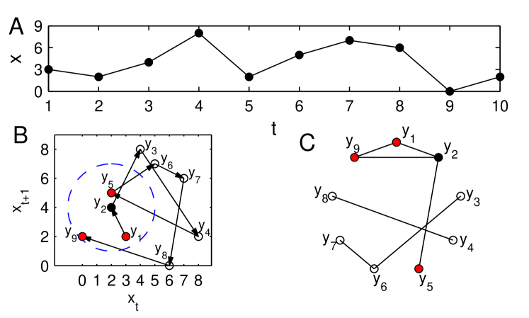
Figure 1: (Colour online) Construction of a RN: (A) time series $x_{t}$, (B) reconstructed two-dimensional phase space trajectory with state vectors $\mathbf{y}_{t}=(x_{t},x_{t+1})$ and an exemplary $\varepsilon$-ball around $y_{2}$ (dashed) for $\varepsilon=3$. (C) Resulting recurrence network.

2 Power-law scaling and singularities of the invariant density

As initial examples, Fig. 2 illustrates the presence of power-law degree distributions in the RNs obtained for several prototypical low-dimensional chaotic systems with a suitable choice of the systems’ characteristic parameters: (i) the Rössler system in spiral-chaos regime: $\dot{x}=-y-z$, $\dot{y}=x+0.2y$, $\dot{z}=0.2+z(x-5.7)$; (ii) the Lorenz system: $\dot{x}=10(y-x)$, $\dot{y}=x(r-z)-y$, $\dot{z}=xy-8/3z$; and (iii) the Hénon map: $x_{n+1}=1-1.4x_{n}^{2}+y_{n}$, $y_{n+1}=0.3x_{n}$. For the Rössler and Lorenz systems, a proper time discretisation has been used as explained in detail in the figure caption.

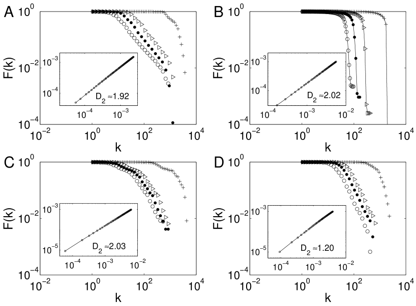
Figure 2: Cumulative degree distributions $F(k)=\sum_{k^{\prime}=k}^{\infty}P(k^{\prime})$ of the RNs obtained for several discrete maps: (A) $x$-component of the first return map of the Rössler system ($\gamma=2.16\pm 0.03$), (B) map of consecutive local maxima of the $z$-component of the Lorenz system with $r=28$ (no scaling), (C) as in (B) with $r=90$ ($\gamma=2.64\pm 0.18$), and (D) Hénon map ($\gamma=2.88\pm 0.04$). Estimates of $\gamma>1$ have been obtained from the cumulative degree distributions $F(k)\sim k^{1-\gamma}$ (in the following figures, we show either $F(k)$ or $P(k)$ when sufficiently straight in a log-log plot) by means of a maximum likelihood approach [21] as averages considering 100 different values of $\rho$ for which a power-law appears. For each $\rho$, $5$ different realisations with random initial conditions are used. We consider RNs of size $N=2\times 10^{5}$ and the Euclidean norm in all examples discussed in this Letter. Four cases were chosen for illustration corresponding to a link density of $\rho_{1}=0.02\%\ (\circ)$, $\rho_{2}=0.03\%\ (\bullet)$, $\rho_{3}=0.05\%\ (\triangleright)$, and $\rho_{4}=3\%\ (+)$. A power-law is hardly detectable for $\rho_{4}$. Insets: corresponding log-log plot of the correlation sum $C(\varepsilon)$ vs. $\varepsilon$, where the correlation dimension $D_{2}$ is estimated by linear regression and agrees well with values from the literature [22, 23, 24].

In all cases, scaling emerges only if the distance threshold $\varepsilon$ is chosen small enough, which corresponds to a small average degree $\langle k\rangle$ and link density $\rho=\langle k\rangle/(N-1)$ of the resulting network ($N$ being the number of nodes). We note that the respective range of $\varepsilon$ should be sufficiently higher than the threshold for which a giant component exists [25]. The size of the scaling regime decreases with growing $\rho$ and becomes hardly detectable for $\rho\gtrsim 1\%$ (Fig. 2). The distance threshold $\varepsilon$ also occurs in dimension estimation where the limit $\varepsilon\to 0$ is taken (e.g., [26]). In contrast, a RN is based on one finite $\varepsilon$. Our smallest $\varepsilon$ are, however, still large enough to avoid the problem of lack of neighbours [23] since the correlation integral $C(\varepsilon)$ still shows the same dependency on $\varepsilon$ as for larger values (see insets in Fig. 2).

A theoretical explanation of the emergence of power-law distributions of RN-based degree is based on the general theory of random geometric graphs [19], where nodes are sampled from some probability density function $p(x)$. For a RN, the space is the phase space of a dynamical system and the nodes are states sampled at discrete times. If we assume that the system is ergodic, the sampled trajectory is already close to its attractor, and the sampling times are generic (particularly, the sampling interval is co-prime to any period lengths of the system), the nodes can be interpreted as being sampled from the probability density function $p(x)$ of the invariant measure $\mu$ of the attractor [27]. The degree distribution of a general random geometric graph, $P(k)$, is derived from $p(x)$ in the limit of large network size $N$ as [19]

$$P(k)=\int dx\,p(x)e^{-\alpha p(x)}(\alpha p(x))^{k}/k!$$ (1)

with $\alpha=\langle k\rangle/\int dx\,p(x)^{2}$ (note that the computation of $\langle k\rangle$ involves integration of $p(x)$ over the $\varepsilon$-neighbourhood of all points $x$ and thus implicitly depends on the specifically chosen $\varepsilon$ as well as the sample size $N$). Hence, the invariant density of the system exclusively determines the existence of a power-law in $P(k)$ and its exponent $\gamma$.

For systems with a one-dimensional phase space, it can be shown that under some weak conditions on $p(x)$ it holds:

$$\textstyle P(k)\approx\frac{k+1}{\alpha}\sum_{x\in p^{-1}(\frac{k+1}{\alpha})}|p^{\prime}(x)|^{-1}.$$ (2)

This implies that if $p(x)$ has a power-law-shaped peak at some state $x_{0}$, i.e., $p(x)\sim|x-x_{0}|^{-1/\gamma}$ for some $\gamma>0$, the degree distribution $P(k)$ also follows a power-law but with the reciprocal exponent, $P(k)\sim k^{-\gamma}$. Specifically, a slower decaying invariant density leads to a faster decaying degree distribution. Note that not all invariant densities lead to power-laws: If $p(x)$ is Gaussian, we get $P(k)\approx 2(-2\ln{k\sqrt{2\pi}/\alpha})^{-1/2}$ instead of a power-law.

More generally, we can deduce that the presence of singularities in the invariant density is the key feature determining whether or not the resulting RN has a power-law degree distribution. This relationship can be intuitively understood: If $p(x)$ has a singularity at some point $x_{0}$ in phase space, then a time series of the associated dynamical system will return very often to the neighbourhood of $x_{0}$. Hence, nodes with a high degree will accumulate close to the singularity. If the resulting invariant density obeys a power-law decay, Eq. (2) implies the emergence of a power-law degree distribution. If there is more than one singularity of $p(x)$, one can expect the resulting degree distribution being related to a weighted sum of the influences of these points. Vice versa, the presence of a power-law degree distribution in the RN of a dynamical system requires the existence of a power-law in the invariant density, i.e., the presence of a singularity. We therefore conjecture that a local power-law in the invariant density is a necessary and sufficient condition for the emergence of a scale-free RN. Beyond the explicit results for one-dimensional systems as discussed above, we further show below that the emergence of a power-law scaling is also possible in higher dimensions and conjecture that this requires the presence of a dynamically invariant object (e.g., an unstable or hyperbolic fixed point) close to which the invariant density scales as a power-law at least in one direction.

3 Power-law scaling vs. fractal dimension

As an example for discrete-time systems leading to power-laws, consider the generalised logistic map [28]

$$f(x)=1-|2x-1|^{\beta}$$ (3)

with $\beta\geqslant\frac{1}{2}$. For $\beta=\frac{1}{2},1,2$, this gives the cusp map, tent map, and standard logistic map, respectively. For general $\beta>0$, the unit interval $[0,1]$ is mapped onto itself by a symmetric function with a maximum of $1$ at $x=\frac{1}{2}$, thus having two pre-images for each $x<1$. For $\beta>1$, the associated invariant density $p(x)$ has two peaks at $x=0$ and $x=1$ with $p(\delta)=p(1-\delta)\sim\delta^{(1-\beta)/\beta}$ for small $\delta$. Hence, the degree distribution $P(k)$ shows a power-law with the exponent

$$\textstyle\gamma=\beta/(\beta-1).$$ (4)

Numerical results shown in Fig. 3A for several different values of $\beta$ agree precisely with Eq. (4).

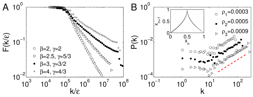
Figure 3: (Colour online) (A): Cumulative degree distribution $F(k)$ of the RNs for the map (3) with $\beta=2,2.5,3,4$. Note that we divide the degree $k$ by $\varepsilon$ so that the $x$-axis is $\varepsilon$-dimensionless. (B) $P(k)$ of the cusp map $\beta=0.5$. The inset shows the corresponding iterative function $f(x)$. The dashed line of (B) has a slope of $1$. The legend indicates the respective link densities $\rho$.

In contrast, for $\beta=1$ the nodes are uniformly distributed, and the degree distribution derived from Eq. (1) is Poissonian, $P(k)=e^{-\alpha}\alpha^{k}/k!$ [29]. For $\beta=\frac{1}{2}$, we get $p(x)=2-2x$ [30, 31], which leads to a specific type of “power-law” in $P(k)$ with $\gamma=-1$ as shown in Fig. 3B. These results imply that the scaling exponent is not simply related to the fractal dimension: the attractor has the box-counting dimension $D_{0}=1$ independently of $\beta$, whereas $\gamma$ changes with varying $\beta$ (Eq. (4)). However, the correlation dimension $D_{2}$ also depends on $\beta$ ($D_{2}=1$ for $\beta\leq 2$, and $D_{2}=2/\beta$ if $\beta>2$ [23]), i.e., there is an indirect relationship between $\gamma$ and $D_{2}$ for certain special cases. The different behaviour of the mentioned dimensions results from the fact that $D_{0}$ exclusively considers the number of boxes required for covering the attractor, but not their individual probability masses as $D_{2}$ and other notions of fractal dimensions do.

Turning to continuous-time systems, we next compare the above findings with those for some discretised standard examples. On the one hand, for the Rössler system, we consider the successive $x$-values when passing the Poincaré section at $y=0$ with $\dot{y}<0$. As shown in the inset of Fig. 4A, the resulting first return map has a shape similar to the case of $\beta=1.87$ in Eq. (3). Hence, we expect a power-law with the exponent $\gamma\approx 1.87/(1.87-1)=2.15$. The invariant density has several dominant peaks, which are together responsible for the power-law observed in Fig. 2A with $\gamma$ indeed close to $2.15$. In fact, $P(k)$ is a mixture of individual power-laws corresponding to the individual peaks of $p(x)$, whose exponents are all roughly the same. On the other hand, for the Lorenz system, we obtain a one-dimensional map by studying the local maxima $z_{max}^{n}$ of $z$ for successive cycles [32], i.e., mapping $z_{max}^{n}$ to $z_{max}^{n+1}$ (inset of Fig. 4B). For $r=28$, this first return map has a similar shape as Eq. (3) for $\beta=0.5$ (inset of Fig. 3B), but the corresponding density is bell-shaped without a peak. Indeed, we do not observe a power-law for $P(k)$ in this case (Fig. 2B). However, increasing $r$ changes the shape of $p(x)$ qualitatively. For example, at $r=90$ (Fig. 4C) the density has peaks at several points, explaining the observed power-law in Fig. 2C. A similar behaviour can be observed for the Hénon map, though the marginal invariant density of the $x$-component has a more complex structure (Fig. 4D).

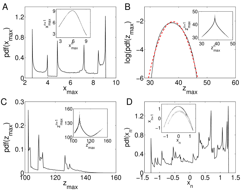
Figure 4: (Colour online) PDF of (A) the successive $x$ values passing the plane of $y=0$ of the Rössler attractor, (B,C) PDF of $z_{max}$ for the Lorenz system of $r=28$ (B) and $r=90$ (C), and (D) marginal density of the $x$ component of the Hénon map. The insets show the associated first return plot. The dashed curve in (B) shows a fit by a Gaussian distribution.

While there is no unambiguous relationship between $\gamma$ and the fractal dimension already for discrete systems, the situation becomes even more complicated for continuous-time systems which are not discretised via a Poincaré section or otherwise. For two-dimensional flows $\dot{x}=\Phi(x)$ with only one peak in $p(x)$, the respective type of behaviour depends on the eigenvalues of the Jacobian $D\Phi(x_{0})$ at the fixed point $x_{0}$ as well as on the shape of $p(x)$. Specifically, in many cases (that shall not be further discussed here) the existence of a power-law for $P(k)$ cannot be evaluated easily, whereas in other cases, one can analytically derive a power-law with a very small exponent of $\gamma=1$. In turn, the following numerical results suggest that there are also examples displaying a distinct relationship between $\gamma$ and some suitably defined local dimension:

For the Rössler system in the regime of screw-type chaos with a homoclinic point at the origin fulfilling the Shilnikov condition [33, 34], the invariant density is dominated by its peak at the origin. The degree distribution $P(k)$ of the corresponding RN shows a power-law with $\gamma\approx 1.33$, which agrees fairly well with the $\vartheta$-capacity dimension $D_{0}^{\vartheta}$ defined in [26] (Fig. 5).

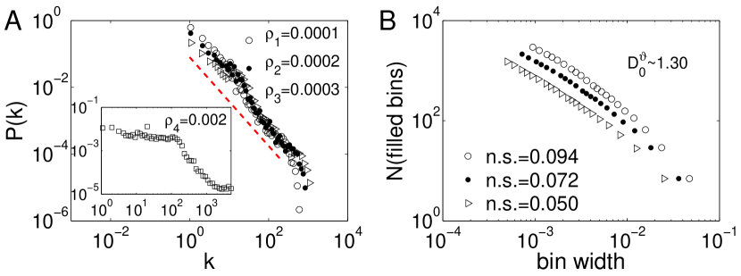
Figure 5: (Colour online) (A): $P(k)$ for the RN of the Rössler system with screw-type chaos [34]. Three different link densities are chosen for illustration as indicated by the legend, a larger link density $\rho_{4}$ does not produce a power-law (inset). The slope of the dashed line is $-1.33$. (B): $\vartheta$-capacity dimension $D_{0}^{\vartheta}\approx 1.30$ in three small cuboidal neighbourhoods of different size (in terms of phase space distance in each coordinate direction, see the legend).

We also observe similar scaling laws for both numerical model and experimental data (output intensities) of a single-mode $\text{CO}_{2}$ laser [35]. The underlying system has a saddle-focus $S$ embedded in the chaotic attractor (Fig. 6A) which causes a spiking dynamics [36, 37]. The attractor is dominated by a homoclinic orbit emerging from and converging to $S$.

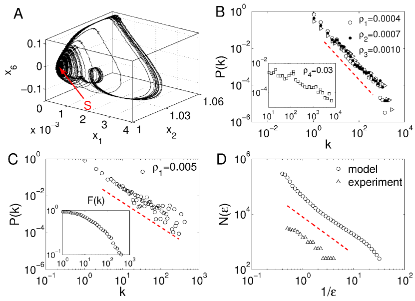
Figure 6: (Colour online) Experimental laser data: (A) Phase portrait in subspace of $(x_{1},x_{2},x_{6})$, where the saddle focus $S$ is at the most dense region. (B) $P(k)$ of RNs from model data for three different link densities (see the legend); a larger link density $\rho_{4}$ does not lead to a power-law (inset). (C) $P(k)$ of RNs from experimental data (inset: cumulative distribution $F(k)$). (D) Point-wise dimension $D_{1}^{S}=1.35$. All dashed lines have slope $-1.35$.

The degree distributions $P(k)$ resulting from both model and experimental data suggest power-laws with $\gamma\approx 1.35$ (Fig. 6B), which qualitatively agrees well with the point-wise dimension of the attractor around $S$. Finally, similar results can be obtained for a predator-prey food-chain model with four competing species [38], which also displays homoclinic chaos, where we observe $\gamma\approx 1.9$ in agreement with $D_{0}^{\vartheta}$ (Fig. 7). This variety of examples underlines the general importance and wide applicability of our findings.

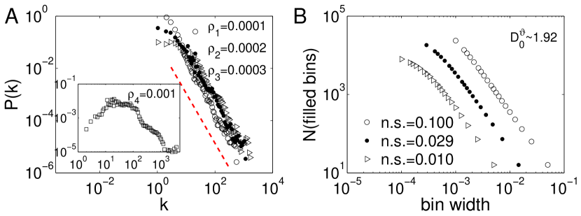
Figure 7: (Colour online) As in Fig. 5 for the Lotka-Volterra system [38] with homoclinic chaos. The slope of the dashed line in panel (A) is $-1.90$.

4 Technical aspects

In general, we have to make two cautionary notes on the numerical study of scaling laws in RNs.

First, in the previous continuous-time examples, the presence of power-laws with the numerically estimated exponents (see above) cannot be rejected on a 90% significance level using Kolmogorov-Smirnov tests. However, the alternative of a power-law with $\gamma=1$ can also not be rejected at the same level. Hence, power-laws with qualitatively different exponents describe the data comparably well. It remains an open problem to determine the correct $\gamma$. We note that this is a general problem when evaluating hypothetical power-laws from finite data [21, 39].

Second, experimental data often consist of only one measured variable. Hence, a reconstruction of the associated phase space trajectory is necessary prior to RN analysis, e.g., by time-delay embedding [40]. Like estimates of dynamical invariants or complexity measures [41, 42], the power-law behaviour of $P(k)$ can depend on the particular observable, because different coordinates of a dynamical system often have different marginal densities. Specifically, embedding theorems ensure topological invariance (i.e., properties of the dynamical system that do not change under smooth coordinate transformations are preserved), but no metric invariance of the attractor’s geometry including $p(x)$. For example, the logistic map and the tent map ($\beta=2,1$ in Eq. (3), respectively) are topologically equivalent under the transformation $x\mapsto\sin^{2}(\pi x/2)$, but the different invariant densities with respect to their original coordinates (that have been used for constructing the RNs from metric distances in their respective phase spaces) lead to distinct scaling exponents $\gamma$ (Fig. 3A).

5 Conclusions

In summary, we have reported an interesting novel aspect of the geometrical organisation underlying the dynamics of many complex systems in physics and beyond. Specifically, we have provided an analytical explanation of the emergence of power-laws in recurrence networks constructed from sampled time series based on the theory of random geometric graphs. Unlike for comparable complex network approaches [10, 11], this scaling is not simply related to the system’s fractal dimension, but determined by both the singularities of the invariant density and the considered spatial scale $\varepsilon$. We emphasise that dimensions are defined in the limit of $\varepsilon\to 0$ and practically estimated by a series of $\varepsilon$ values, whereas the power-law exponent $\gamma$ of the RN appears for each sufficiently small $\varepsilon$ individually. Note that in contrast to the degree, the transitivity properties of RNs have a direct relationship with attractor dimension [43].

In comparison with the invariant density itself, fractal dimensions are a rather specific characteristic. In particular, they do not simply describe the whole system (as the invariant density itself does), but quantify density variations on the attractor viewed at different spatial scales $\varepsilon$ [26, 44]. Conversely, the scaling exponent $\gamma$ directly characterises a power-law decay of the density in phase space independent of a specific scale. In this spirit, both fractal dimension and scaling exponent $\gamma$ capture conceptually different aspects of the geometric organisation of a dynamical system in its phase space. However, although there is no general relationship between $\gamma$ and fractality, in some special cases the power-law exponent coincides with some notion of dimension. This has been demonstrated for several example systems as well as experimental data. In turn, we have found that in other cases the value of $\gamma$ drops to $1$. Further studies are necessary in order to better understand this complex relationship between power-law degree distributions and fractal scaling (i.e. under which general conditions related to a system’s structural organisation both scaling exponent and fractal dimension coincide), particularly in continuous dynamical systems.

From a conceptual perspective, we would like to remark that studying a single scalar property like the scaling exponent of a recurrence network or the fractal dimension cannot provide a complete view on the structural organisation of a nonlinear complex system. Specifically, both characteristics capture distinct and complementary features related to the probability density of the invariant measure. In this spirit, the power-law exponent $\gamma$ quantifies a fundamental property that has not been explicitly studied so far. Because its relationship with the features of possible singularities of the invariant density is intuitive (i.e. the emergence of power-law degree distributions has some clear physical meaning), one particular strength of studying the degree distribution of recurrence networks is that it potentially allows identifying the presence of such singularities in complex situations (e.g., for observational data).

6 Acknowledgements

This work was partially supported by the German BMBF and the Leibniz association (projects PROGRESS and ECONS) as well as the German National Academic Foundation. We acknowledge constructive comments by C. Grebogi and M. Zaks.

References

- [1] \NameGutenberg B. Richter C. F. \REVIEWBull. Seism. Soc. Am.341944185.
- [2] \NameMantegna R. N. Stanley H. E. \REVIEWNature376199546.
- [3] \NameFarmer J. D. Lillo F. \REVIEWQuant. Finance420047.
- [4] \NameAlbert R. Barabasi A.-L. \REVIEWRev. Mod. Phys.74200247.
- [5] \NameNewman M. E. J. \REVIEWSIAM Rev.452003167.
- [6] \NameGao J., Buldyrev S., Stanley H. Havlin S. \REVIEWNature Physics8201240.
- [7] \NameDonges J. F., Schultz H. C. H., Marwan N., Zou Y. Kurths J. \REVIEWEur. Phys. J. B842011635.
- [8] \NameBoccaletti S., Latora V., Moreno Y., Chavez M. Hwang D.-U. \REVIEWPhys. Rep.4242006175.
- [9] \NameArenas A., Diaz-Guilera A., Kurths J., Moreno Y. Zhou C. \REVIEWPhys. Rep.469200893.
- [10] \NameZhang J. Small M. \REVIEWPhys. Rev. Lett.962006238701.
- [11] \NameLacasa L., Luque B., Ballesteros F., Luque J. Nuno J. C. \REVIEWProc. Natl. Acad. Sci.10520084972.
- [12] \NameXu X., Zhang J. Small M. \REVIEWProc. Natl. Acad. Sci.105200819601.
- [13] \NameMarwan N., Donges J. F., Zou Y., Donner R. V. Kurths J. \REVIEWPhys. Lett. A37320094246.
- [14] \NameDonner R. V., Zou Y., Donges J. F., Marwan N. Kurths J. \REVIEWNew J. Phys.122010033025.
- [15] \NameDonner R. V., Zou Y., Donges J. F., Marwan N. Kurths J. \REVIEWPhys. Rev. E812010015101(R).
- [16] \NameDonges J. F., Donner R. V., Trauth M. H., Marwan N., Schellnhuber H. J. Kurths J. \REVIEWProc. Natl. Acad. Sci.108201120422.
- [17] \NamePoincaré H. \REVIEWActa Mathematica131890A3.
- [18] \NameMarwan N., Romano M. C., Thiel M. Kurths J. \REVIEWPhys. Rep.4382007237.
- [19] \NameHerrmann C., Barthélemy M. Provero P. \REVIEWPhysical Review E682003026128.
- [20] \NameBarthélemy M. \REVIEWPhys. Rep.49920111 .
- [21] \NameClauset A., Shalizi C. R. Newman M. E. J. \REVIEWSIAM Rev.512009661.
- [22] \NameGrassberger P. Procaccia I. \REVIEWPhys. Rev. Lett.501983346.
- [23] \NameSprott J. C. \BookChaos and Time-Series Analysis (Oxford University Press, Oxford) 2003.
- [24] \NameKantz H. Schreiber T. \BookNonlinear time series analysis (Cambridge University Press) 1997.
- [25] \NameDonges J. F., Heitzig J., Donner R. V. Kurths J. \REVIEWPhys. Rev. Esubm..
- [26] \NameFarmer J. D., Ott E. Yorke J. A. \REVIEWPhysica D71983153.
- [27] \NameEckmann J. P. Ruelle D. \REVIEWRev. Mod. Phys.571985617.
- [28] \NameLyra M. L. Tsallis C. \REVIEWPhys. Rev. Lett.80199853.
- [29] \NameDall J. Christensen M. \REVIEWPhys. Rev. E662002016121.
- [30] \NameGyörgyi G. Szépfalusy P. \REVIEWZ. Phys. B551984179.
- [31] \NameHemmer P. C. \REVIEWJ. Phys. A171984L247.
- [32] \NameLorenz E. \REVIEWJ. Atmos. Sci.201963130.
- [33] \NameShilnikov L. \REVIEWMath. USSR Sbornik10197091.
- [34] \NameGaspard P. Nicolis G. \REVIEWJ. Stat. Phys.311983499.
- [35] \NamePisarchik A. N., Meucci R. Arecchi F. T. \REVIEWEur. Phys. J. D132001385.
- [36] \NameChannell P., Cymbalyuk G. Shilnikov A. \REVIEWPhys. Rev. Lett.982007134101.
- [37] \NameArecchi F. T., Meucci R. Gadomski W. \REVIEWPhys. Rev. Lett.5819872205.
- [38] \NameVano J., Wildenberg J., Anderson M., Noel J. Sprott J. \REVIEWNonlinearity1920062391.
- [39] \NameStumpf M. P. H. Porter M. A. \REVIEWScience3352012665.
- [40] \NamePackard N. H., Crutchfield J. P., Farmer J. D. Shaw R. S. \REVIEWPhys. Rev. Lett.451980712.
- [41] \NameLetellier C., Aguirre L. A. Maquet J. \REVIEWPhys. Rev. E712005066213.
- [42] \NameLetellier C. \REVIEWPhys. Rev. Lett.962006254102.
- [43] \NameDonner R. V., Heitzig J., Donges J. F., Zou Y., Marwan N. Kurths J. \REVIEWEur. Phys. J. B842011653.
- [44] \NameHalsey T. C., Jensen M. H., Kadanoff L. P., Procaccia I. Shraiman B. I. \REVIEWPhys. Rev. A3319861141.