Minimax estimation for mixtures of Wishart distributions

Abstract

The space of positive definite symmetric matrices has been studied extensively as a means of understanding dependence in multivariate data along with the accompanying problems in statistical inference. Many books and papers have been written on this subject, and more recently there has been considerable interest in high-dimensional random matrices with particular emphasis on the distribution of certain eigenvalues. With the availability of modern data acquisition capabilities, smoothing or nonparametric techniques are required that go beyond those applicable only to data arising in Euclidean spaces. Accordingly, we present a Fourier method of minimax Wishart mixture density estimation on the space of positive definite symmetric matrices.

, , and

t2Supported in part by the Natural Sciences and Engineering Research Council of Canada, Grant DG 46204.

t3Supported in part by Basic Science Research Program through the National Research Foundation of Korea (NRF) funded by the Ministry of Education, Science and Technology (2011-0027601).

t4Supported in part by NSF Grant DMS-07-05210.

1 Introduction

The space of positive definite symmetric matrices has been studied extensively in statistics as a means of understanding dependence in multivariate data along with the accompanying problems in statistical inference. Many books and papers, for example, haff1 , haff2 , haff3 , loh , Muirhead , stein-rietz and stein , have been written on this subject, and there has been considerable interest recently in high-dimensional random matrices with particular emphasis on the distribution of certain eigenvalues johnstone08 and on graphical models lm .

In this paper we consider the problem of estimating the mixing density of a continuous mixture of Wishart distributions. We construct a nonparametric estimator of that density and obtain minimax rates of convergence for the estimator. Throughout this work, we adopt, as a guide, results developed for the classical problem of deconvolution density estimation on Euclidean spaces; see, for example, diggle , fan , Koo , mr , butsy and Zhang . Much of the difficulty with the space of positive definite symmetric matrices is due to the fact that mathematical analysis on the space is technically demanding. Helgason he2 and Terras Terras-II provide much insight and technical innovation, however, and we make extensive use of these methods.

We summarize the paper as follows. In Section 2 we discuss and set up the notation for Wishart mixtures. In Section 3 we begin by reviewing the necessary Fourier methods which allow us to construct a nonparametric estimator of the mixing density, and then we provide the estimator. The minimax property of our nonparametric estimator is stated in Section 4 along with supporting results. Section 5 presents simulation results as well as an application to finance examining real financial data. Finally, Sections 6 and 7 present the proofs.

2 Wishart mixtures

Throughout the paper, for any square matrix $y$, we denote the trace and determinant of $y$ by $\operatorname{tr}y$ and $|y|$, respectively; further, we denote by ${\mathbf{I}}_{m}$ the $m\times m$ identity matrix. We will denote by ${\mathcal{P}_{m}}$ the space of $m\times m$ positive definite symmetric matrices.

For $s=(s_{1},\ldots,s_{m})\in\mathbb{C}^{m}$ with $\operatorname{Re}(s_{j}+\cdots+s_{m})>(j-1)/2$, $j=1,\ldots,m$, the multivariate gamma function is defined as

$$\Gamma_{m}(s_{1},\ldots,s_{m})=\pi^{m(m-1)/4}\prod_{j=1}^{m}\Gamma\biggl{(}s_{j}+\cdots+s_{m}-\frac{1}{2}(j-1)\biggr{)},$$ (1)

where $\Gamma(\cdot)$ denotes the classical gamma function.

We denote by $G$ the general linear group $\operatorname{GL}(m,\mathbb{R})$ of all $m\times m$ nonsingular real matrices, by $K$ the group ${\mathrm{O}}(m)$ of $m\times m$ orthogonal matrices and by $A$ the group of diagonal positive definite matrices. The group $G$ acts transitively on ${\mathcal{P}_{m}}$ by the action

$$G\times{\mathcal{P}_{m}}\to{\mathcal{P}_{m}},\qquad(g,y)\mapsto g^{\prime}yg,$$ (2)

$g\in G$, $y\in{\mathcal{P}_{m}}$, where $g^{\prime}$ denotes the transpose of $g$. Under this group action, the isotropy group of the identity in $G$ is $K$; hence the homogeneous space $K\setminus G$ can be identified with ${\mathcal{P}_{m}}$ by the natural mapping from $K\setminus G\to{\mathcal{P}_{m}}$ that sends $Kg\mapsto g^{\prime}g$. In distinguishing between left and right cosets, we place the quotient operation on the left and right of the group, respectively.

For $y=(y_{ij})\in{\mathcal{P}_{m}}$, define the measure

$${\mathrm{d}_{*}}y=|y|^{-(m+1)/2}{\prod_{1\leq i\leq j\leq m}dy_{ij}}.$$

It is well known that the measure ${\mathrm{d}_{*}}y$ is invariant under action (2). Relative to the dominating measure ${\mathrm{d}_{*}}y$, the probability density function of the standard Wishart distribution with $N$ degrees of freedom is

$$w(y)=\frac{1}{2^{Nm/2}\Gamma_{m}(0,\ldots,0,N/2)}|y|^{N/2}\exp\biggl{(}-\frac{1}{2}\operatorname{tr}y\biggr{)},$$ (3)

$y\in{\mathcal{P}_{m}}$. Consequently, for $\sigma\in{\mathcal{P}_{m}}$, we note that $\operatorname{tr}(\sigma^{-1/2}y\sigma^{-1/2})=\operatorname{tr}(\sigma^{-1}y)$ and $|\sigma^{-1/2}y\sigma^{-1/2}|=|\sigma^{-1}y|$. It then follows that, relative to the dominating measure ${\mathrm{d}_{*}}y$, the density of the general Wishart distribution, with covariance parameter $\sigma$, is $w(\sigma^{-1}y)$, $y\in{\mathcal{P}_{m}}$.

Suppose next that $\sigma$ is a random matrix and, relative to the dominating measure ${\mathrm{d}_{*}}\sigma$, has a continuous mixing density, $f$, that is invariant under the action (2). By integration with respect to $\sigma$, the continuous Wishart mixture density is given by

$$r(y)=\int_{{\mathcal{P}_{m}}}f(\sigma)w(\sigma^{-1}y)\,{\mathrm{d}_{*}}\sigma,$$ (4)

$y\in{\mathcal{P}_{m}}$. For the case in which $m=1$, the standard Wishart density is essentially a chi-square density, in which case (4) is a continuous mixture of chi-square densities.

In general, (4) is a convolution operation for functions on ${\mathcal{P}_{m}}$. We denote by $x^{1/2}$ any matrix with $x^{t/2}x^{1/2}=x$, where $x^{t/2}=(x^{1/2})^{\prime}$ and denote $x^{-t/2}=(x^{-1/2})^{t}$. Define $X\circ Z$, the convolution of two random matrices $X$ and $Z$ which are distributed on ${\mathcal{P}_{m}}$ by

$$X\circ Z=X^{t/2}ZX^{1/2}$$

and $f_{1}*f_{2}$, the convolution of $f_{1}\in L^{1}({\mathcal{P}_{m}})$ and $f_{2}\in L^{1}({\mathcal{P}_{m}})$ by

$$(f_{1}*f_{2})(y)=\int_{\mathcal{P}_{m}}f_{1}(x)f_{2}(x^{-t/2}yx^{-1/2})\,{\mathrm{d}_{*}}x\qquad\mbox{for }y\in{\mathcal{P}_{m}},$$

where $L^{q}({\mathcal{P}_{m}})$ is the space of integrable functions raised to the $q$th power on ${\mathcal{P}_{m}}$ for $q\geq 1$. If $X$ and $Z$ with densities $f$ and $w$, respectively, are independent, then $Y=X\circ Z$ has the density $r=f*w$ since $w(\sigma^{-t/2}y\sigma^{-1/2})=w(\sigma^{-1}y)$. Finally, (4) can be transformed into a scalar multiplication; see Section 3.2.

3 Fourier analysis on ${\mathcal{P}_{m}}$ and estimation of the mixing density

In this section we review the Fourier methods needed to transform the convolution product (4) and to construct a nonparametric estimator of the mixing density $f$.

3.1 The Helgason–Fourier transform

For $y\in{\mathcal{P}_{m}}$, denote by $|y_{j}|$ the principal minor of order $j$, $j=1,\ldots,m$. For $s\in\mathbb{C}^{m}$, the power function $p_{s}\dvtx\allowbreak{\mathcal{P}_{m}}\to\mathbb{C}$ is

$$p_{s}(y)=\prod_{j=1}^{m}|y_{j}|^{s_{j}},$$ (5)

$y\in{\mathcal{P}_{m}}$. Let ${\mathrm{d}_{*}}k$ denote the Haar measure on $K$, normalized to have total volume equal to one; then

$$h_{s}(y)=\int_{K}p_{s}(k^{\prime}yk)\,{\mathrm{d}_{*}}k,$$ (6)

$y\in{\mathcal{P}_{m}}$, is the zonal spherical function on ${\mathcal{P}_{m}}$. It is well known that the functions $h_{s}$ are fundamental to harmonic analysis on symmetric spaces he2 , Terras-II . If $s_{1},\ldots,s_{m}$ are nonnegative integers then, up to a constant factor, (6) is an integral formula for the zonal polynomials which arise in many aspects of multivariate statistical analysis Muirhead , pages 231 and 232.

Let $C_{c}^{\infty}({\mathcal{P}_{m}})$ denote the space of infinitely differentiable, compactly supported, complex-valued functions $f$ on ${\mathcal{P}_{m}}$; also, let

$$C_{c}^{\infty}({\mathcal{P}_{m}}/K)=\{f\in C_{c}^{\infty}({\mathcal{P}_{m}})\dvtx f(k^{\prime}yk)=f(y)\mbox{ for all }k\in K,y\in{\mathcal{P}_{m}}\}.$$

For $s\in\mathbb{C}^{m}$ and $k\in K$, the Helgason–Fourier transform (Terras-II , page 87) of a function $f\in C_{c}^{\infty}({\mathcal{P}_{m}})$ is

$${\mathcal{H}}f(s,k)=\int_{{\mathcal{P}_{m}}}f(y){\overline{p_{s}(k^{\prime}yk)}}\,{\mathrm{d}_{*}}y,$$ (7)

where ${\overline{p_{s}(k^{\prime}yk)}}$ denotes complex conjugation.

For the case in which $f\in C_{c}^{\infty}({\mathcal{P}_{m}}/K)$, we make the change of variables $y\mapsto k_{1}^{\prime}yk_{1}$ in (7), $k_{1}\in K$, and integrate with respect to the Haar measure ${\mathrm{d}_{*}}k_{1}$. Applying the invariance of $f$ and formula (6), we deduce that ${\mathcal{H}}f(s,k)$ does not depend on $k$. Specifically, ${\mathcal{H}}f(s,k)=\hat{f}(s)$ where

$$\hat{f}(s)=\int_{{\mathcal{P}_{m}}}f(y){\overline{h_{s}(y)}}\,{\mathrm{d}_{*}}y,$$ (8)

$s\in\mathbb{C}^{m}$, is the zonal spherical transform of $f$.

In the case of the standard Wishart density (3), which is a $K$-invariant function, the zonal spherical transform is well known (Muirhead Muirhead , page 248; Terras Terras-II , pages 85 and 86):

$$\hat{w}(s)=\frac{\Gamma_{m}(s_{m-1},\ldots,s_{1},-(s_{1}+\cdots+s_{m})+N/2)}{\Gamma_{m}(0,\ldots,0,N/2)}h_{s}\biggl{(}\frac{1}{2}{\mathbf{I}}_{m}\biggr{)}.$$

3.2 The convolution property of the Helgason–Fourier transform

The following result shows that the convolution operation can be transformed into a scalar multiplication.

Proposition 3.1

Suppose $X$ and $Z$ with densities $f_{X}$ and $f_{Z}$, respectively, are independent, and $Z$ is $K$-invariant. Let $f_{Y}$ be the density of $Y=X\circ Z$. Then

$${\mathcal{H}}f_{Y}(s,k)={\mathcal{H}}f_{X}(s,k)\hat{f}_{Z}(s)\qquad\mbox{for }s\in\mathbb{C}^{m}\mbox{ and }k\in K.$$

Note

$${\mathcal{H}}f_{Y}(s,k)=\mathbb{E}p_{\bar{s}}(k^{\prime}Yk)=\mathbb{E}p_{\bar{s}}(k^{\prime}X^{t/2}ZX^{1/2}k).$$

Using the $KAN$-Iwasawa decomposition of $X^{t/2}k$ (Terras Terras-II , page 20), we have $X^{1/2}k=HU$ for $H\in K$ and $U$, an upper triangular matrix. Observe

$$\mathbb{E}p_{\bar{s}}(k^{\prime}X^{t/2}ZX^{1/2}k) = \mathbb{E}_{X}\{p_{\bar{s}}(U^{\prime}U)\mathbb{E}_{Z|X}p_{\bar{s}}(H^{\prime}ZH)\}$$

$$= \hat{f}_{Z}(s)\mathbb{E}_{X}\{p_{\bar{s}}(U^{\prime}U)\}$$

$$= {\mathcal{H}}f_{X}(s,k)\hat{f}_{Z}(s),$$

where Proposition 1 of Terras Terras-II , page 39, is used for the first equality.

3.3 The inversion formula for the Helgason–Fourier transform

For $a_{1},\allowbreak a_{2}\in\mathbb{C}$ with $\operatorname{Re}(a_{1}),\operatorname{Re}(a_{2})>0$, let

$$B(a_{1},a_{2})=\frac{\Gamma(a_{1})\Gamma(a_{2})}{\Gamma(a_{1}+a_{2})}$$

denote the classical beta function. For $s\in\mathbb{C}^{m}$ such that $\operatorname{Re}(s_{i}+\cdots+s_{j})>-\frac{1}{2}(j-i+1)$ for all $1\leq i<j\leq m-1$, the Harish–Chandra $c$-function is

$$c_{m}(s)=\prod_{1\leq i<j\leq m-1}\frac{B(1/2,s_{i}+\cdots+s_{j}+(j-i+1)/2)}{B(1/2,(j-i+1)/2)}.$$ (9)

Let $\rho\equiv(\frac{1}{2},\ldots,\frac{1}{2},\frac{1}{4}(1-m))$, and set

$$\omega_{m} = \frac{\prod_{j=1}^{m}\Gamma(j/2)}{(2\pi i)^{m}\pi^{m(m+1)/4}m!},$$ (10)

$$\mathbb{C}^{m}(\rho) = \{s\in\mathbb{C}^{m}\dvtx\operatorname{Re}(s)=-\rho\}$$ (11)

and

$${\mathrm{d}_{*}}s=\omega_{m}|c_{m}(s)|^{-2}\,{\mathrm{d}_{*}}s_{1}\cdots{\mathrm{d}_{*}}s_{m}.$$

Let $M=\{{\operatorname{diag}}(\pm 1,\ldots,\pm 1)\}$ be the set of $m\times m$ diagonal matrices with entries $\pm 1$ on the diagonal; then $M$ is a subgroup of $K$ and is of order $2^{m}$. By factorizing the Haar measure ${\mathrm{d}_{*}}k$ on $K$, it may be shown (Terras-II , page 88) that there exists an invariant measure ${\mathrm{d}_{*}}\bar{k}$ on the coset space $K/M$ such that

$$\int_{\bar{k}\in K/M}{\mathrm{d}_{*}}\bar{k}=1.$$

The inversion formula for the Helgason–Fourier transform ${\mathcal{H}}$ in (8) is that if $f\in C^{\infty}_{c}({\mathcal{P}_{m}})$, then he2 , Terras-II

$$f(y)=\int_{\mathbb{C}^{m}(\rho)}\int_{\bar{k}\in K/M}{\mathcal{H}}f(s,k)p_{s}(k^{\prime}yk)\,{\mathrm{d}_{*}}\bar{k}\,{\mathrm{d}_{*}}s,$$ (12)

$y\in{\mathcal{P}_{m}}$. In particular, if $f\in C^{\infty}_{c}({\mathcal{P}_{m}}/K)$, then

$$f(y)=\int_{\mathbb{C}^{m}(\rho)}\hat{f}(s)h_{s}(y)\,{\mathrm{d}_{*}}s,$$

$y\in{\mathcal{P}_{m}}$, and there also holds the Plancherel formula,

$$\int_{{\mathcal{P}_{m}}}|f(y)|^{2}\,{\mathrm{d}_{*}}y=\int_{\mathbb{C}^{m}(\rho)}\int_{K/M}|{\mathcal{H}}f(s,k)|^{2}\,{\mathrm{d}_{*}}\bar{k}\,{\mathrm{d}_{*}}s.$$ (13)

We refer to Terras Terras-II , page 87 ff., for full details of the inversion formula and for references to the literature.

3.4 Eigenvalues, the Laplacian and Sobolev spaces

For $y=(y_{ij})\in{\mathcal{P}_{m}}$, we define the $m\times m$ matrix of partial derivatives,

$$\frac{\partial}{\partial y}=\biggl{(}\frac{1}{2}(1+\delta_{ij})\,\frac{\partial}{\partial y_{ij}}\biggr{)},$$

where $\delta_{ij}$ denotes Kronecker’s delta. The Laplacian, $\Delta$, on ${\mathcal{P}_{m}}$ can be written (Terras-II , page 106) in terms of the local coordinates $y_{ij}$ as

$$\Delta=-\operatorname{tr}\biggl{(}\biggl{(}y\,\frac{\partial}{\partial y}\biggr{)}^{2}\biggr{)}.$$

The power function $p_{s}$ in (5) is an eigenfunction of $\Delta$ (see Muirhead , page 229, Richards1 , page 283, Terras-II , page 49). Indeed, let $r_{j}=s_{j}+s_{j+1}+\cdots+s_{m}+\frac{1}{4}(m-2j+1)$, $j=1,\ldots,m$, and define

$$\lambda_{s}=-(r_{1}^{2}+\cdots+r_{m}^{2})+\tfrac{1}{48}m(m^{2}-1);$$ (14)

then $\Delta p_{s}(Y)=\lambda_{s}p_{s}(Y)$. Since $\operatorname{Re}(s)=-\rho$ then each $r_{j}$, $j=1,\ldots,m$, is purely imaginary; hence, $\lambda_{s}>0$, $s\in C_{m}(\rho)$.

The operator ${\mathcal{H}}$ changes the effect of invariant differential operators on functions to pointwise multiplication: if $f\in C^{\infty}_{c}({\mathcal{P}_{m}})$, then

$${\mathcal{H}}(\Delta f)(s,k)=\lambda_{s}{\mathcal{H}}f(s,k),$$

$s\in\mathbb{C}^{m}$, $k\in K$ (Terras-II , page 88). For $\varphi>0$, we therefore define the fractional power, $\Delta^{\varphi/2}$, of $\Delta$, as the operator such that

$${\mathcal{H}}(\Delta^{\varphi/2}f)(s,k)=\lambda_{s}^{\varphi/2}{\mathcal{H}}f(s,k),$$

$f\in C^{\infty}_{c}({\mathcal{P}_{m}})$. Having constructed $\Delta^{\varphi/2}$, we define the Sobolev class,

$${{\mathcal{F}}_{\varphi}}=\{f\in C^{\infty}({\mathcal{P}_{m}})\dvtx\|\Delta^{\varphi/2}f\|^{2}<\infty\},$$

where for $f\in C^{\infty}({\mathcal{P}_{m}})$,

$$\|f\|=\biggl{(}\int_{{\mathcal{P}_{m}}}|f(y)|^{2}\,{\mathrm{d}_{*}}y\biggr{)}^{1/2}$$

denotes the $L^{2}({\mathcal{P}_{m}})$-norm with respect to the measure ${\mathrm{d}_{*}}y$. For $Q>0$, we also define the bounded Sobolev class,

$${{\mathcal{F}}_{\varphi}}(Q)=\{f\in C^{\infty}({\mathcal{P}_{m}})\dvtx\|\Delta^{\varphi/2}f\|^{2}<Q\}.$$

4 Main result

In this section we will present the main result. We do so by applying the Helgason–Fourier transform to the mixture density (4) so that

$${\mathcal{H}}r(s,k)={\mathcal{H}}f(s,k)\hat{w}(s),$$ (15)

$s\in\mathbb{C}^{m}$, $k\in K$; see Proposition 3.1. Having observed a random sample $Y_{1},\allowbreak\ldots,Y_{n}$ from the mixture density, $r$, in (4), we estimate ${\mathcal{H}}r(s,k)$ by its empirical Helgason–Fourier transform,

$${{\mathcal{H}}_{n}r}(s,k)=\frac{1}{n}\sum_{\ell=1}^{n}\overline{p_{s}(k^{\prime}Y_{\ell}k)}.$$ (16)

On substituting (16) in (15), together with the assumption that $\hat{w}(s)\neq 0$, $s\in\mathbb{C}^{m}$, we obtain

$${{\mathcal{H}}_{n}f}(s,k)=\frac{{\mathcal{H}}_{n}r(s,k)}{{\hat{w}}(s)},$$

$s\in\mathbb{C}^{m}$, $k\in K$.

Analogous with classical Euclidean deconvolution, we introduce a smoothing parameter $T=T(n)$ where $T(n)\to\infty$ as $n\to\infty$, and then we apply the inversion formula (12) using a spectral cut-off based on the eigenvalues of $\Delta$. First, we introduce the notation

$$\mathbb{C}^{m}(\rho,T)=\{s\in\mathbb{C}^{m}(\rho)\dvtx\lambda_{s}<T\},$$

where $\mathbb{C}^{m}(\rho)$ is defined in (11). We now define

$$f_{n}(y)=\int_{\mathbb{C}^{m}(\rho,T)}\int_{\bar{k}\in K/M}\frac{{\mathcal{H}}_{n}r(s,\bar{k})}{{\hat{w}}(s)}p_{s}(\bar{k}^{\prime}y\bar{k})\,{\mathrm{d}_{*}}\bar{k}\,{\mathrm{d}_{*}}s,$$ (17)

$y\in{\mathcal{P}_{m}}$, and take this as our nonparametric estimator of $f$.

We now state the minimax result for the estimator (17). Let $C$ denote a generic positive constant independent of $n$. For two sequences of real numbers $\{a_{n}\}$ and $\{b_{n}\}$, we use the notations $a_{n}\ll b_{n}$ and $a_{n}\gg b_{n}$ to mean $a_{n}<Cb_{n}$ and $a_{n}>Cb_{n}$, respectively, as $n\to\infty$. Moreover, $a_{n}\asymp b_{n}$ means that $a_{n}\ll b_{n}$ and $a_{n}\gg b_{n}$.

Theorem 4.1

Suppose $f$ is a density on ${\mathcal{P}_{m}}$ and $N>(m-1)/2$. Then, for the Wishart mixture (4),

$$\sup_{f\in{{\mathcal{F}}_{\varphi}}(Q)}\mathbb{E}\|f_{n}-f\|^{2}\ll(\log n)^{-2\varphi}$$ (18)

and for any estimator $g_{n}$ of $f$,

$$\inf_{g_{n}}\sup_{f\in{{\mathcal{F}}_{\varphi}}(Q)}\mathbb{E}\|g_{n}-f\|^{2}\gg(\log n)^{-2\varphi}.$$ (19)

We now provide some comments about this result. In the situation where (4) is a finite sum, so that

$$r(y)=\sum_{\ell=1}^{q}f_{\ell}w(\sigma_{\ell}^{-1}y)\quad\mbox{and}\quad\sum_{\ell=1}^{q}f_{\ell}=1,$$

we have the finite mixture model. Methods for recovering the mixing coefficients can be covered by the techniques employed in chentan . We note that the continuous mixture model is a generalization of this approach.

It is noted that the condition $f$ is a density and seems to be mild. The upper bound property of (18) is established in kr2 , Theorem 3.3, with $\beta=1/2$. In the latter, the moment condition

$$\int_{{\mathcal{P}_{m}}}|y_{1}|^{-1}\cdots|y_{m-1}|^{-1}|y|^{(m-1)/2}r(y)\,{\mathrm{d}_{*}}y<\infty,$$ (20)

on the principal minors $|y_{1}|,\ldots,|y_{m}|$ of $y\in{\mathcal{P}_{m}}$ is assumed. In our theorem, we did not impose this moment condition as condition (20) is automatically satisfied. This is pointed out and commented upon below in the proof.

To derive the lower bound for estimating $f$ in the $L^{2}({\mathcal{P}_{m}})$-norm, we shall follow the standard Euclidean approach. Thus we choose a pair of functions $f^{0}$, $f^{n}\in{{\mathcal{F}}_{\varphi}}(Q)$, and, with $w$ denoting the Wishart density (3), we shall show that, for some constants $C_{1},C_{2}>0$,

$$\|f^{n}-f^{0}\|^{2}\geq C_{1}(\log n)^{-2\varphi}$$

and

$$\chi^{2}(f^{0}*w,f^{n}*w)\leq\frac{C_{2}}{n},$$ (21)

where

$$\chi^{2}(g_{1},g_{2})=\int_{{\mathcal{P}_{m}}}\frac{(g_{1}(y)-g_{2}(y))^{2}}{g_{1}(y)}\,{\mathrm{d}_{*}}y.$$

Precisely, let us suppose we can choose $f^{0}\in{{\mathcal{F}}_{\varphi}}(Q)$ and a perturbation $\psi\in{{\mathcal{F}}_{\varphi}}(Q)$, and, for $\delta=\delta_{n}>0$, let $\psi^{\delta}$ be a scaling of $\psi$ such that $\|\psi^{\delta}\|\asymp\delta^{-1/2}\|\psi\|$. Define

$$f^{n}=f^{0}+C_{\psi}\delta^{-\varphi+1/2}\psi^{\delta}.$$

If $\delta$ can be chosen so that

$$\chi^{2}(f^{0}*w,f^{n}*w)\leq Cn^{-1},$$

then the lower bound rate of convergence is determined by $\delta^{-2\varphi}$. We shall develop such a construction and, moreover, do so in a way such that $\delta\asymp\log n$ as $n\to\infty$.

Remark 4.2.

The profound influence of Charles Stein on covariance estimation originates largely from his Rietz lecture; see stein-rietz . The idea is that for certain loss functions over ${\mathcal{P}_{m}}$, the usual estimator of the covariance matrix parameter is inadmissible. Through an unbiased estimation of the risk function over covariance matrices, Stein was able to improve upon the usual estimator by pooling the observed eigenvalues of the sample covariance matrix. Subsequent to this, through a series of papers, improvements were obtained in Haff haff1 , haff2 , haff3 . Other related works include Takemura takemura , Lin and Perlman linperl and Loh loh , to name a few.

In this paper, we contribute to the case in which one observes data from a continuous mixture of Wishart distributions, not merely a sample from a single distribution. Therefore, the parameter of interest would be the mixing density of the covariance parameters. And the nonparametric estimator of the mixing density (17) is an attractive candidate because of its minimax property. Based on this procedure, one could consider the moment, or mode, of $f_{n}$, as a possible estimator of the corresponding population parameters. Alternatively, one could take a nonparametric empirical Bayes approach as in Pensky pensky .

5 Numerical aspects and an application to finance

This section presents numerical aspects for the $m=2$ case with an application to finance.

5.1 Computation of estimators

Suppose $X$ and $Z$ are independentwith $Z$ having a Wishart distribution. Let $Y=X^{t/2}ZX^{1/2}$ where $X^{1/2}$ is upper triangular. For visualization, we display estimators of the marginal density for $D$ where $X=H^{\prime}DH$ with $H\in K$ and $D\in A$. Let

$$\hat{r}_{n}(s)=\frac{1}{n}\sum_{j=1}^{n}\overline{h_{s}(E_{j})}\quad\mbox{and}\quad\hat{f}_{n}(s)=\frac{\hat{r}_{n}(s)}{\hat{w}(s)},$$

where $E_{j}\in A_{+}$ denotes the diagonal matrix of eigenvalues of $Y_{j}$, $j=1,\ldots,n$. Denote by $f^{D}$ the density of eigenvalues of $X$. Then, the estimator for $f^{D}$ is given by

$$\qquad f^{D}_{n}(a)=\int_{\mathbb{C}^{2}(\rho,T)}\operatorname{Re}\{\hat{f}_{n}(s)h_{s}(a)\}\,{\mathrm{d}_{*}}s\qquad\mbox{for }a=\operatorname{diag}(a_{1},a_{2})\in A.$$ (22)

Consider the computation of $h_{s}(a)$ when

$$s=-\rho+ib=(-1/2+ib_{1},1/4+ib_{2})$$

so that $\operatorname{Re}(s)=-\rho$. From pages 90 and 91 of Terras-II , the spherical function is given by

$$h_{s}(a)=(a_{1}a_{2})^{i(b_{2}+b_{1}/2)}P_{-1/2+ib_{1}}\bigl{(}\cosh\bigl{(}\log\bigl{(}\sqrt{a_{1}/a_{2}}\bigr{)}\bigr{)}\bigr{)},$$

where Legendre function $P_{-1/2+it}(x)$ can be computed using conicalP_0(t, x) in the gsl library in R.

The mean integrated squared error (MISE) of $f^{D}_{n}$ is defined by

$$\operatorname{MISE}(f_{n})=\mathbb{E}\int_{A}\bigl{(}f^{D}_{n}(a)-f^{D}(a)\bigr{)}^{2}\,{\mathrm{d}_{*}}a.$$

It is reasonable to choose $T$ which minimizes $\operatorname{MISE}(f^{D}_{n})$ or equivalently

$$M(T)=\mathbb{E}\int_{A}(f^{D}_{n}(a))^{2}\,{\mathrm{d}_{*}}a-2\mathbb{E}\int_{A}f^{D}_{n}(a)f^{D}(x)\,{\mathrm{d}_{*}}a.$$

One can find an unbiased estimator $M_{0}(T)$ of $M(T)$; see kkkoz . We choose $\hat{T}$ by

$$\mathop{\arg\min}_{T}M_{0}(T).$$

Monte Carlo approximation is used for integration of (22) and $M_{0}(T)$.

5.2 Simulation

Denote by $W_{N}(\sigma)$ the Wishart density with degrees of freedom $N$ and covariance matrix $\sigma$. We generate data as follows. For $j=1,\ldots,n$:

• generate $Z_{j}\sim W_{20}(I_{2})$;

• generate $X_{j}\sim f$;

• do a Cholesky decomposition of $X_{j}=(X_{j})^{t/2}(X_{j})^{1/2}$, and calculate $Y_{j}=(X_{j})^{t/2}Z_{j}(X_{j})^{1/2}$.

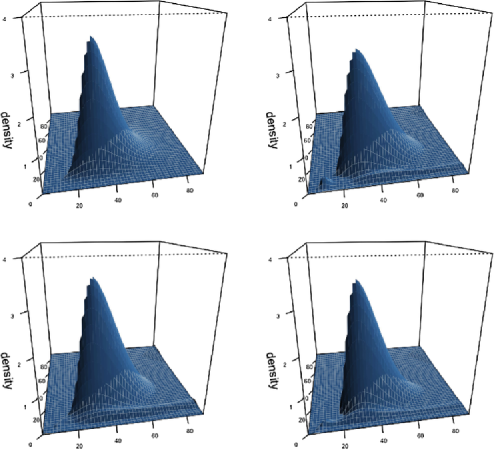
Figure 1: Unimodal case: upper left displays the true density of $W_{15}(2I_{2})$, upper right shows an estimate with $n=500$, lower left with $n=1\mbox{,}000$ and lower right with $n=2\mbox{,}000$.

As examples, we consider a unimodal mixing density $W_{15}(2I_{2})$ and a bimodal density $0.5W_{15}(2I_{2})+0.5W_{15}(6I_{2})$. Figure 1 show the results for the unimodal case whereas Figure 2 show the results for the bimodal case. In each of these plots the

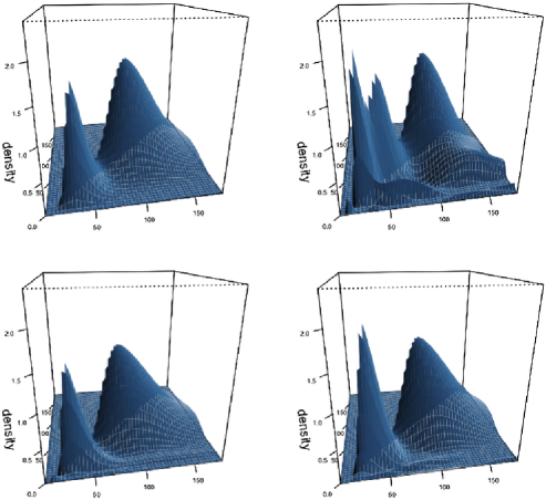
Figure 2: Bimodal case: upper left displays the true density $0.5W_{15}(2I_{2})+0.5W_{15}(6I_{2})$, upper right shows an estimate with $n=500$, lower left with $n=1\mbox{,}000$ and lower right with $n=2\mbox{,}000$.

domain consists of the two eigenvalues starting with the largest. One can see that the general shapes of the estimators become closer to that of the true density as $n$ increases.

5.3 Application to stochastic volatility

Stochastic volatility using the Wishart distribution is of much interest in finance; see, for example, amu and gs . In particular, this entails a situation precisely of the form (4). Let us apply this to the situation where we are interested in estimating the mixing density.

Although our methods can be applied to a portfolio of many assets, let us restrict ourselves to two assets since this would be the smallest multivariate example. Indeed, let $S^{1}_{j}$ and $S^{2}_{j}$ denote the daily closing stock prices of Samsung Electronics (005930.KS) and LG-display (034220.KS), respectively, traded on the Korea Stock Exchange (KSC) for 2010, where the data can be easily accessed on public financial websites. We will assume as usual that $Q^{k}_{j}=\log(S^{k}_{j+1}/S^{k}_{j})$ follows a bi-variate normal distribution for $k=1,2$. We transform the daily data to weekly data and compute the weekly $2\times 2$ covariance matrix $Y_{i}$ for $i=1,\ldots,52$. In case a week has a holiday, we repeat the last previous observation. Under the usual assumptions this would constitute observations from a mixture model (4) with a standard Wishart distribution with four degrees of freedom.

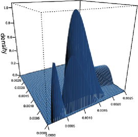
Figure 3: A density estimator for the weekly covariance matrix of stock prices.

Figure 3 plots the mixing density estimator corresponding to the two eigenvalues. One can see that there are two peaks, suggesting a possible bimodal stochastic volatility mixing density in the eigenvalues.

6 Proof of upper bound

The strategy here is, first, to decompose the integrated mean-squared error into its variance and bias components,

$$\mathbb{E}\|f_{n}-f\|^{2} = \mathbb{E}\|(f_{n}-\mathbb{E}f_{n})+(\mathbb{E}f_{n}-f)\|^{2}$$

$$= \mathbb{E}\|f_{n}-\mathbb{E}f_{n}\|^{2}+\|\mathbb{E}f_{n}-f\|^{2},$$

and, last, to estimate each component separately using estimates based on the Plancherel formula and the inversion formula for the Helgason–Fourier transform.

6.1 The integrated bias

Lemma 6.1

Suppose that $f\in{{\mathcal{F}}_{\varphi}}(Q)$ and $\varphi>\dim{\mathcal{P}_{m}}/2$. Then

$$\|\mathbb{E}f_{n}-f\|^{2}\ll T^{-\varphi}.$$

We have for $x\in{\mathcal{P}_{m}}$

$$\quad\mathbb{E}f_{n}(x)-f(x) = \int_{\mathbb{C}^{m}(\rho,T)}\int_{\bar{k}\in K/M}{\mathcal{H}}f(s,\bar{k})p_{s}(\bar{k}^{\prime}x\bar{k})\,{\mathrm{d}_{*}}\bar{k}\,{\mathrm{d}_{*}}s$$

$${}-\int_{\mathbb{C}^{m}(\rho)}\int_{\bar{k}\in K/M}{\mathcal{H}}f(s,\bar{k})p_{s}(\bar{k}^{\prime}x\bar{k})\,{\mathrm{d}_{*}}\bar{k}\,{\mathrm{d}_{*}}s$$

$$= -\int_{\lambda_{s}>T,\operatorname{Re}(s)=-\rho}\int_{\bar{k}\in K/M}{\mathcal{H}}f(s,\bar{k})p_{s}(\bar{k}^{\prime}x\bar{k})\,{\mathrm{d}_{*}}\bar{k}\,{\mathrm{d}_{*}}s.$$

Applying the Plancherel formula, we obtain

$$\|\mathbb{E}f_{n}-f\|^{2}=\int_{\lambda_{s}>T,\operatorname{Re}(s)=-\rho}\int_{K/M}|{\mathcal{H}}f(s,\bar{k})|^{2}\,{\mathrm{d}_{*}}\bar{k}\,{\mathrm{d}_{*}}s.$$

Consequently,

$$\|\mathbb{E}f_{n}-f\|^{2} = \int_{\lambda_{s}\geq T,\operatorname{Re}(s)=-\rho}\int_{K/M}|{\mathcal{H}}f(s,\bar{k})|^{2}\,{\mathrm{d}_{*}}\bar{k}\,{\mathrm{d}_{*}}s$$

$$\leq T^{-\varphi}\int_{\lambda_{s}\geq T,\operatorname{Re}(s)=-\rho}\int_{K/M}\lambda_{s}^{\varphi}|{\mathcal{H}}f(s,\bar{k})|^{2}\,{\mathrm{d}_{*}}\bar{k}\,{\mathrm{d}_{*}}s$$

$$\leq T^{-\varphi}\int_{\mathbb{C}^{m}(\rho)}\int_{K/M}\lambda_{s}^{\varphi}|{\mathcal{H}}f(s,\bar{k})|^{2}\,{\mathrm{d}_{*}}\bar{k}\,{\mathrm{d}_{*}}s,$$

where we use the fact that

$$\lambda_{s}^{\varphi}|{\mathcal{H}}f(s,k)|^{2}\equiv|\lambda_{s}^{\varphi/2}{\mathcal{H}}f(s,k)|^{2}=|{\mathcal{H}}(\Delta^{\varphi/2}f)(s,k)|^{2}.$$

Therefore

$$\|\mathbb{E}f_{n}-f\|^{2} \leq T^{-\varphi}\int_{\mathbb{C}^{m}(\rho)}\int_{\bar{k}\in K/M}|{\mathcal{H}}(\Delta^{\varphi/2}f)(s,k)|^{2}\,{\mathrm{d}_{*}}\bar{k}\,{\mathrm{d}_{*}}s$$

$$= T^{-\varphi}\int_{{\mathcal{P}_{m}}}|\Delta^{\varphi/2}f(w)|^{2}\,{\mathrm{d}_{*}}w,$$

where the equality follows from the Plancherel formula. By assumption, $f\in{{\mathcal{F}}_{\varphi}}(Q)$, the latter integral is bounded above by $Q$, so we obtain

$$\|\mathbb{E}f_{n}-f\|^{2}\leq QT^{-\varphi},$$

and the proof is complete.

6.2 The integrated variance

To obtain bounds for the integrated variance, several preliminary calculations are needed. In particular, we begin with the variance calculation of the empirical Helgason–Fourier transform, which has similarities to the usual empirical characteristic function.

Lemma 6.2

For $s\in\mathbb{C}^{m}(\rho)$ and $k\in K/M$,

$$\mathbb{E}|{\mathcal{H}}_{n}r(s,k)-\mathbb{E}{\mathcal{H}}_{n}r(s,k)|^{2}=\frac{1}{n}\bigl{(}|{\mathcal{H}}r(-2\rho,k)|^{2}-|{\mathcal{H}}r(s,k)|^{2}\bigr{)}.$$

By (16),

$$|{\mathcal{H}}_{n}r(s,k)|^{2} = \overline{{\mathcal{H}}_{n}r(s,k)}{\mathcal{H}}_{n}r(s,k)$$

$$= \frac{1}{n^{2}}\sum_{j,\ell=1}^{n}\overline{p_{s}(k^{\prime}Y_{j}k)}p_{s}(kY_{\ell}k)$$

$$= \frac{1}{n^{2}}\Biggl{\{}\sum_{j=1}^{n}|p_{s}(k^{\prime}Y_{j}k)|^{2}+\sum_{j\neq\ell}\overline{p_{s}(k^{\prime}Y_{j}k)}p_{s}(k^{\prime}Y_{\ell}k)\Biggr{\}}.$$

Observe also that

$$p_{s}(w)\overline{p_{s}(w)} = |w_{1}|^{s_{1}}\cdots|w_{m}|^{s_{m}}\overline{|w_{1}|^{s_{1}}\cdots|w_{m}|^{s_{m}}}$$

$$= |w_{1}|^{2\operatorname{Re}(s_{1})}\cdots|w_{m}|^{2\operatorname{Re}(s_{m})}$$

$$= p_{-2\rho}(w)$$

since $\operatorname{Re}(s)=-\rho$. Applying this result to (6.2) and taking expectations, we obtain

$$\mathbb{E}|{\mathcal{H}}_{n}r(s,k)|^{2} = \frac{1}{n^{2}}\mathbb{E}\Biggl{\{}\sum_{j=1}^{n}|p_{s}(k^{\prime}Y_{j}k)|^{2}+\sum_{j\neq\ell}\overline{p_{s}(k^{\prime}Y_{j}k)}p_{s}(k^{\prime}Y_{\ell}k)\Biggr{\}}$$

$$= \frac{1}{n^{2}}\Biggl{\{}\sum_{j=1}^{n}\mathbb{E}p_{-2\rho}(k^{\prime}Y_{j}k)+\sum_{j\neq\ell}\overline{\mathbb{E}p_{s}(k^{\prime}Y_{j}k)}\mathbb{E}p_{s}(k^{\prime}Y_{\ell}k)\Biggr{\}}$$

$$= \frac{1}{n}{\mathcal{H}}r(-2\rho,k)+\frac{n-1}{n}|{\mathcal{H}}r(s,k)|^{2},$$

where the last equality follows from the fact that $Y_{1},\ldots,Y_{n}$ are independent and identically distributed as $Y$, and because $\mathbb{E}p_{s}(k^{\prime}Yk)={\mathcal{H}}r(s,k)$.

Following Terras Terras-II , pages 34 and 35, let

$$A^{+}=\{a=\operatorname{diag}(a_{1},\ldots,a_{m})\in A\dvtx a_{1}>\cdots>a_{m}\}$$

denote the positive Weyl chamber in $A$. For $a=\operatorname{diag}(a_{1},\ldots,a_{m})\in A$, let $\mathrm{d}a=\prod_{j=1}^{m}a_{j}^{-1}da_{j}$ and set

$$\gamma(a)=\prod_{j=1}^{m}a_{j}^{-(m-1)/2}\prod_{1\leq i<j\leq m}|a_{i}-a_{j}|,$$

and define the normalizing constant $b_{m}$ by $b_{m}^{-1}=\pi^{-(m^{2}+m)/4}\prod_{j=1}^{m}j\Gamma(j/2)$. Denote ${\mathrm{d}_{*}}a=b_{m}\gamma(a)\,\mathrm{d}a$.

Lemma 6.3

As $T\to\infty$,

$$\mathbb{E}\|f_{n}-\mathbb{E}f_{n}\|^{2}\ll{\sup_{s\in\mathbb{C}^{m}(\rho)}}|\hat{w}_{Z}(s)|^{-2}\frac{T^{\dim{\mathcal{P}_{m}}/2}}{n}.$$

By the Plancherel formula,

$$\mathbb{E}\|f_{n}-\mathbb{E}f_{n}\|^{2}$$

$$\qquad=\int_{\mathbb{C}^{m}(\rho,T)}\int_{K/M}\mathbb{E}|{\mathcal{H}}_{n}f(s,k)-\mathbb{E}{\mathcal{H}}_{n}f(s,k)|^{2}\,\mathrm{d}\bar{k}\,{\mathrm{d}_{*}}s$$

$$\qquad=\int_{\mathbb{C}^{m}(\rho,T)}\int_{K/M}\mathbb{E}|{\mathcal{H}}_{n}r(s,k)-\mathbb{E}{\mathcal{H}}_{n}r(s,k)|^{2}\,\mathrm{d}\bar{k}|\hat{w}_{Z}(s)|^{-2}\,{\mathrm{d}_{*}}s$$

$$\qquad\leq\frac{1}{n}\sup_{\lambda_{s}<T,\operatorname{Re}(s)=-\rho}|\hat{w}_{Z}(s)|^{-2}\int_{K/M}|{\mathcal{H}}r(-2\rho,\bar{k})|^{2}\,\mathrm{d}\bar{k}\int_{\mathbb{C}^{m}(\rho,T)}{\mathrm{d}_{*}}s$$

$$\qquad\ll{\sup_{\lambda_{s}<T,\operatorname{Re}(s)=-\rho}}|\hat{w}_{Z}(s)|^{-2}\frac{T^{\dim{\mathcal{P}_{m}}/2}}{n}$$

as $T\to\infty$.

Choose $a\in A^{+}$. Observe that

$$p_{-2\rho}(a)=a_{1}^{-(m-1)+(m-1)/2}\cdots a_{m-1}^{-1+(m-1)/2}a_{m}^{(m-1)/2}\leq 1.$$ (27)

Since $p_{-2\rho}(k^{\prime}ak)$ is a continuous function of $k$ on a compact set $K$, $p_{-2\rho}(k^{\prime}ak)$ is uniformly bounded on $K$ such $|p_{-2\rho}(k^{\prime}ak)|\leq C$ on $K$. Since $f$ is a density so that $r$ is also a density, we have

$$|{\mathcal{H}}r(-2\rho,{\mathbf{I}}_{m})| = \biggl{|}\int_{\mathcal{P}_{m}}r(y)\overline{p_{-2\rho}(y)}\,{\mathrm{d}_{*}}y\biggr{|}$$

$$= \int_{A^{+}}\int_{K}r(k^{\prime}ak)\overline{p_{-2\rho}(k^{\prime}ak)}\,{\mathrm{d}_{*}}a\,{\mathrm{d}_{*}}k$$

$$\leq \int_{A^{+}}\int_{K}r(k^{\prime}ak)|\overline{p_{-2\rho}(k^{\prime}ak)}|\,{\mathrm{d}_{*}}a\,{\mathrm{d}_{*}}k$$

$$\leq C\int_{A^{+}}\int_{K}r(k^{\prime}ak)\,{\mathrm{d}_{*}}a\,{\mathrm{d}_{*}}k$$

$$= C\int_{\mathcal{P}_{m}}r(y)\,{\mathrm{d}_{*}}y$$

$$= C.$$

Hence, it follows from continuity and the compactness of $K/M$

$$\int_{K/M}|{\mathcal{H}}r(-2\rho,\bar{k})|^{2}\,\mathrm{d}\bar{k}<\infty,$$

which has been used in the above calculation.

In addition, we use the fact that, as $T\to\infty$,

$${\sup_{\mathbb{C}^{m}(\rho,T)}}|c_{m}(s)|^{-2}\ll T^{m(m-1)/4},$$

a result which follows from Proposition 7.2 of Helgason he2 , page 450.

The proof of the upper bound can now be obtained by applying Lemmas 6.1 and 6.3 to (6) and setting $T\asymp(\log n)^{2}$.

7 Proof of lower bound

We need to provide some detailed calculations, and the essence of the proof is contained for the case $m=2$; hence we will keep this assumption for the remainder of this paper. The generalization to $m>2$ may be obtained by using higher order hyperbolic spherical coordinates. In this section, we assume that $\psi$ is a $K$-invariant function defined on ${\mathcal{P}_{2}}$.

7.1 Convolution and Helagson–Fourier transform in polar coordinate

For $y\in{\mathcal{P}_{2}}$, let $y=k^{\prime}ak$ with $a=\operatorname{diag}(a_{1},a_{2})\in A^{+}$, $k\in K$ so that $\psi(y)=\psi(a)$. Let

$$a=D_{u_{1}}e^{u_{2}}$$

with $D_{z}=\operatorname{diag}(e^{z},e^{-z})$ for $z\in\mathbb{R}$, and write

$$\psi(u)=\psi(D_{u_{1}}e^{u_{2}}).$$

By a change of variables,

$$\int_{{\mathcal{P}}_{2}}\psi(y)\,{\mathrm{d}_{*}}y=\int_{{{\mathcal{D}}}}\psi(u)\,{\mathrm{d}_{*}}u,$$ (28)

where

$${{\mathcal{D}}}=\{u\dvtx u_{1}\in\mathbb{R}^{+}\mbox{ and }u_{2}\in\mathbb{R}\}$$

and

$${\mathrm{d}_{*}}u=4\pi\sinh u_{1}\,\mathrm{d}u_{1}\,\mathrm{d}u_{2}.$$

Denote $k_{\theta}=\bigl{[}{\cos\theta\atop\sin\theta}\enskip{{-}\sin\theta\atop\cos\theta}\bigr{]}$. The next lemma is straightforward so we shall omit the proof.

Lemma 7.1

For $u_{1}\in\mathbb{R}^{+}$, $v_{1}\in\mathbb{R}^{+}$ and $\theta\in[0,2\pi]$, the matrix equation

$$k_{\xi}D_{R}k_{\xi}^{\prime}=D_{-u_{1}/2}k_{\theta}D_{v_{1}}k_{\theta}^{\prime}D_{-u_{1}/2}$$

has a solution $R^{*}=R^{*}(u_{1},v_{1},\theta)$ and $\xi^{*}=\xi^{*}(u_{1},v_{1},\theta)$. Further, $\cosh R^{*}$ has minimum and maximum values $\cosh(u_{1}-v_{1})$ and $\cosh(u_{1}+v_{1})$, respectively, and $R^{*}$ and $\xi^{*}$ can be defined uniquely.

In general, if both $f$ and $g$ are $K$-invariant functions on ${\mathcal{P}_{m}}$, then $f*g$ is also $K$-invariant and $f*g=g*f$. Hence, $\psi*w$ is $K$-invariant and $\psi*w=w*\psi$ due to $K$-invariance of $\psi$ and $w$. From this and Lemma 7.1, we can define

$$\Psi_{u_{1}v_{1}}(z)=\frac{1}{2\pi}\int_{0}^{2\pi}\psi(R^{*}(\theta,u_{1},v_{1}),z)\,\mathrm{d}\theta$$

for $z\in\mathbb{R}$, $u_{1}\in\mathbb{R}^{+}$, $v_{1}\in\mathbb{R}^{+}$. Denoting by $W$ the distribution function corresponding to the standard Wishart density $w(u)$ with respect to the measure ${\mathrm{d}_{*}}u$, we have that for $v\in D$,

$$(\psi*w)(v)=\int_{{{\mathcal{D}}}}\Psi_{u_{1}v_{1}}(v_{2}-u_{2})\,\mathrm{d}W(u).$$ (29)

The Laplacian for $K$-invariant functions in polar coordinate is given by $\Delta=\Delta_{u_{1}}+\Delta_{u_{2}}$, where

$$\Delta_{u_{1}}=-\coth(u_{1})\frac{\partial}{\partial u_{1}}-\frac{\partial^{2}}{\partial u_{1}^{2}},\qquad\Delta_{u_{2}}=-\frac{\partial^{2}}{\partial u_{2}^{2}},$$

and the spherical function is given by

$$h_{s}(u)=P_{s_{1}}(\cosh u_{1})e^{(s_{1}+2s_{2})u_{2}}\qquad\mbox{for }u\in{{\mathcal{D}}}$$ (30)

with $P_{s}$, the Legendre function; see Terras Terras-II . It can be seen that

$$\Delta_{u_{1}}h_{s}=-\tfrac{1}{2}s(s+1)h_{s},\qquad\Delta_{u_{2}}h_{s}=-\tfrac{1}{2}(s_{1}+2s_{2})^{2}h_{s},$$

so that $\Delta h_{s}=\lambda_{s}h_{s}$ with $\lambda_{s}=-{\frac{1}{2}}\{(s_{1}+2s_{2})^{2}+s(s+1)\}$.

The Helgason–Fourier transform of $\psi$ is given by

$$\hat{\psi}(s)=\int_{{\mathcal{D}}}\psi(u)P_{\bar{s}_{1}}(\cosh u_{1})e^{(\overline{s_{1}+2s_{2}})u_{2}}\,{\mathrm{d}_{*}}u$$ (31)

from (28) and (30). Suppose $\psi$ is separable so that $\psi(u)=\psi_{1}(u_{1})\psi_{2}(u_{2})$. Then, (31) implies

$$\hat{\psi}(s)={\mathcal{M}}\psi_{1}(\bar{s}_{1})\mathcal{L}\psi_{2}(s_{1}+2s_{2}),$$ (32)

where $\mathcal{L}$ and $\mathcal{M}$ denote, respectively, the Laplace transform and the Mehler–Fock transform; see Terras Terras-II .

7.2 $\chi^{2}$-divergence

Choose $\psi_{1}$ as the perturbation function as in Fan fan . Then, one can construct $\psi(u)$ satisfying the following conditions: [(P5)]

$\psi$ is $K$-invariant and separable with $\psi(u)=\psi_{1}(u_{1})\psi_{2}(u_{2})$ for $u\in D$.

$\mathcal{L}\psi_{2}(it)=0$ for $t\notin[1,2]$.

$\psi\in{{\mathcal{F}}_{\varphi}}(Q)$.

$\psi_{1}(u_{1})=O(\cosh^{-m_{0}}u_{1})$ and $\psi_{2}(u_{2})=O(e^{-m_{0}|u_{2}|})$, where $0<\xi<1$ and $m_{0}\xi>(N-1)(1-\xi)/2$.

$\int_{{\mathcal{D}}}\psi(u)\,{\mathrm{d}_{*}}u=0$.

Let $p_{b}$ be a density on $\mathbb{R}$ such that $p_{b}$ is sufficiently smooth and satisfies $p_{b}(u_{2})=c_{b}\exp(-b|u_{2}|)$, $|u_{2}|\geq c_{0}$, where $c_{b}$ is a normalizing constant. Define the function

$$f^{0}(u)=C_{b}(\cosh u_{1})^{-b}p_{b}(u_{2}),$$

where $C_{b}=c_{b}(b-1)/(2\pi)$ for $b>1$.

For a function $g\dvtx{\mathcal{P}_{2}}\rightarrow\mathbb{R}$ and $\delta>0$, define

$$g^{\delta}(y)=g\bigl{(}|y|^{(\delta-1)/2}y\bigr{)}\qquad\mbox{for }y\in{\mathcal{P}_{2}}$$

so that

$$\psi(u)=\psi(u_{1},\delta u_{2})\qquad\mbox{for }u\in{{\mathcal{D}}}.$$

Proposition 7.2

Suppose (P1)–(P5) hold. For a pair of densities

$$f^{0}\quad\mbox{and}\quad f^{n}=f^{0}+C_{\psi}\delta^{-\varphi+1/2}\psi^{\delta},$$

the $\chi^{2}$-divergence between $g^{0}=f^{0}*w$ and $g^{n}=f^{n}*w$ satisfies

$$\chi^{2}(g^{0},g^{n})\leq C/n$$

provided that $b<\frac{1}{2}\min(3\pi,(N-1)(1-\xi)-1)$.

The fact that $(\log n)^{-2\varphi}$ is a lower bound follows from Proposition 7.2 whose proof follows from a sequence of lemmas below.

7.3 Perturbing function

Denote $(q_{1},q_{2})=(s_{1},s_{1}+2s_{2})$ and $\beta_{j}=\operatorname{Im}(q_{j})$ for $j=1,2$. Note that $q_{2}=i\beta_{2}$ for $s\in C^{2}(\rho)$.

Lemma 7.3

Suppose (P1) holds. Then $\|\psi^{\delta}\|=\delta^{-1}\|\psi\|$.

By (32) and the change of variable $u_{2}\mapsto\delta u_{2}$, we obtain

$$\hat{\psi}^{\delta}(s)=\mathcal{M}\psi_{1}(\bar{q}_{1})\{\delta^{-1}\mathcal{L}\psi_{2}(\bar{q}_{2}/\delta)\}.$$

The desired result follows from the Plancherel formula (13) and change of variable $s\mapsto q$.

Lemma 7.4

Suppose (P1), (P2) and (P3) hold. Then there exists a positive constant $C_{\psi}$ such that $C_{\psi}\delta^{-\varphi+1/2}\psi^{\delta}\in{{\mathcal{F}}_{\varphi}}(Q)$.

Suppose $s\in C^{2}(\rho)\cap{\mathcal{S}}$. Observe that

$$\lambda_{s}=-\tfrac 12\{s_{1}(s_{1}+1)+(s_{1}+2s_{2})^{2}\}=\tfrac 12\bigl{(}\beta_{1}^{2}+\beta_{2}^{2}+\tfrac 14\bigr{)}$$

and that for $\delta\geq 1$,

$$\tfrac 12\bigl{(}\beta_{1}^{2}+(\delta\beta_{2})^{2}+\tfrac 14\bigr{)}\leq\delta^{2}\lambda_{s}.$$

Now, the Plancherel formula (13) and change of variable $s\mapsto q$ gives

$$\|\Delta^{\varphi/2}\psi^{\delta}\|^{2}\leq C\delta^{2\varphi-1}\|\Delta^{\varphi/2}\psi\|^{2}.$$

A suitable choice of $C_{\psi}$ gives the desired result.

Lemma 7.5

Under (P1) and (P2), $\|\psi^{\delta}*w\|^{2}\leq C\delta e^{-3\pi\delta}\|\psi\|^{2}$.

For $s\in C^{2}(\rho)\cap{\mathcal{S}}$,

$$|\hat{w}(s)|^{2}\leq Ce^{-\pi(\alpha_{1}+2\alpha_{2})}=Ce^{-2\pi\beta_{2}}\leq Ce^{-3\pi}.$$

The desired result follows from the inequality $e^{-\pi(s_{1}+2s_{2})\delta}\leq Ce^{-3\pi\delta}$, the Plancherel formula (13) and change of variable $s\mapsto q$.

7.4 Tail behavior

Lemma 7.6

For $c_{1}\geq 0$ and $c_{2},c_{3}\in\mathbb{R}$,

$$\int_{\{u_{1}>{c_{1}},c_{2}<u_{2}<c_{3}\}}\mathrm{d}W(u)=4\pi\int_{\{c_{2}<u_{2}<c_{3}\}}\exp\{(N-1)u_{2}-e^{u_{2}}\cosh{c_{1}}\}\,\mathrm{d}u_{2}.$$

Change of variable gives the desired result.

If $U$ has the distribution function $W$, then $(U_{1},\delta U_{2})$ has the distribution function $W_{\delta}$ with density $\delta^{-1}w(u_{1},u_{2}/\delta)$. By (29) and a change of variables,

$$(\psi^{\delta}*w)(v)=\int_{{{\mathcal{D}}}}\Psi_{u_{1}v_{1}}(\delta v_{2}-u_{2})\,\mathrm{d}W_{\delta}(u).$$ (33)

Lemma 7.7

We have $g^{0}=f^{0}*w$ is $K$-invariant, and as $v_{1}\to\infty$ and $|v_{2}|\to\infty$

$$g^{0}(v)\geq Ce^{-b(v_{1}+|v_{2}|)}.$$

Choose a constant $C_{1/2}$ such that

$$\int_{\{0\leq u_{1}<C_{1/2},|u_{2}|<C_{1/2}\}}\mathrm{d}W(u)\geq 1/2$$

and $p_{b}(u_{2})\,{=}\,c_{b}\exp({-}b|u_{2}|)$ for $|u_{2}|\,{\geq}\,C_{1/2}$. The desired result follows from (29) and Lemma 7.1.

Lemma 7.8

Define

$$\eta_{\delta}(v)=\int_{{\mathcal{D}}}\cosh^{-m_{0}}(u_{1}-v_{1})e^{-m_{0}|v_{2}-u_{2}|}\,\mathrm{d}W_{\delta}(u).$$

Then, there exist $M$ and a constant $C$ such that when $v_{1}\geq M$ and $|v_{2}|/\delta\geq M$,

$$\eta_{\delta}(v)\leq C\exp\bigl{\{}-\tfrac 12(N-1)(1-\xi)(v_{1}+|v_{2}|/\delta)\bigr{\}}$$

for all $\delta\geq 1$ provided that $0<\xi<1$ and $m_{0}\xi>(N-1)(1-\xi)/2$.

Denote

$$J_{11} = \{u\dvtx|u_{1}-v_{1}|\leq\xi v_{1},|v_{2}-\delta u_{2}|\leq\xi|v_{2}|\},$$

$$J_{12} = \{u\dvtx|u_{1}-v_{1}|\leq\xi v_{1},|v_{2}-\delta u_{2}|>\xi|v_{2}|\},$$

$$J_{21} = \{u\dvtx|u_{1}-v_{1}|>\xi v_{1},|v_{2}-\delta u_{2}|\leq\xi|v_{2}|\},$$

$$J_{22} = \{u\dvtx|u_{1}-v_{1}|>\xi v_{1},|v_{2}-\delta u_{2}|>\xi|v_{2}|\}$$

and for $i,j=1,2$,

$$I_{ij}=\int_{J_{ij}}\cosh^{-m_{0}}(u_{1}-v_{1})e^{-m_{0}|v_{2}-u_{2}|}\,\mathrm{d}W_{\delta}(u).$$

Consider $I_{11}$. Suppose $v_{2}<0$. If $|u_{1}-v_{1}|\leq\xi v_{1}$ and $|v_{2}-\delta u_{2}|\leq\xi|v_{2}|$, then

$$(1-\xi)(v_{1}+|v_{2}|/\delta)\leq u_{1}-u_{2}\leq(1+\xi)(v_{1}+|v_{2}|/\delta).$$

Let $\zeta=(1-\xi)(v_{1}+|v_{2}|/\delta)$ and $\lambda=e^{\zeta}$. Note that

$$I_{11}\leq C\biggl{(}\int_{\{u_{1}\geq 0,u_{2}<-\zeta\}}\mathrm{d}W(u)+\int_{\{u_{1}\geq u_{2}+\zeta,-\zeta\leq u_{2}<0\}}\mathrm{d}W(u)\biggr{)}:=I_{1}^{-}+I_{2}^{-}.$$

Since $e^{u_{2}}\cosh(u_{2}+\zeta)=\frac{1}{2}(\lambda e^{2u_{2}}+\lambda^{-1}),$ then we have

$$I_{1}^{-}=4\pi\int_{\{0\leq t<1/\lambda\}}t^{N-2}e^{-t}\,\mathrm{d}t=O\bigl{(}\lambda^{-(N-1)}\bigr{)}$$

and by Lemma 7.6 with $c_{1}=u_{2}+\zeta$, $c_{2}=-\zeta$ and $c_{3}=0$

$$I_{2}^{-}=C\int_{\{-\zeta\leq u_{2}<0\}}e^{(N-1)u_{2}}\exp\bigl{(}-e^{u_{2}}\cosh(u_{2}+\zeta)\bigr{)}\,\mathrm{d}u_{2}=O\bigl{(}\lambda^{-(N-1)/2}\bigr{)}.$$

Hence, if $v_{2}\,{<}\,0$, then $I_{11}\,{=}\,O(\lambda^{-(N-1)/2})$ as $v_{1}\,{+}\,|v_{2}|/\delta\,{\to}\,\infty$. Suppose $v_{2}\,{\geq}\,0$. If $|v_{2}-\delta u_{2}|\leq\xi|v_{2}|$ and $|u_{1}-v_{1}|\leq\xi v_{1}$, then

$$(1-\xi)(v_{1}+|v_{2}|/\delta)\leq u_{1}+u_{2}\leq(1+\xi)(v_{1}+|v_{2}|/\delta).$$

Observe that

$$I_{11}\leq C\biggl{(}\int_{\{u_{1}\geq 0,u_{2}\geq\zeta\}}\mathrm{d}W(u)+\int_{\{u_{1}\geq\zeta-u_{2},0\leq u_{2}<\zeta\}}\mathrm{d}W(u)\biggr{)}\\ :=I_{1}^{+}+I_{2}^{+}.$$

Since $e^{u_{2}/2}\cosh(\zeta-u_{2})=\frac{1}{2}(\lambda+\lambda^{-1}e^{2u_{2}})$, then we have

$$I_{1}^{+}=4\pi\int_{\{t\geq\lambda\}}t^{N-2}e^{-t}\,\mathrm{d}t=O(e^{-\lambda})$$

and by Lemma 7.6, with $c_{1}=u_{2}-\zeta$, $c_{2}=0$ and $c_{3}=\zeta$,

$$I_{2}^{+}=C\int_{\{0\leq u_{2}<\zeta\}}e^{(N-1)u_{2}}\exp\bigl{(}-e^{u_{2}}\cosh(\zeta-u_{2})\bigr{)}\,\mathrm{d}u_{2}=O(e^{-\lambda}).$$

Hence, for $v_{2}\in\mathbb{R}$,

$$I_{11}=O\bigl{(}\lambda^{-(N-1)/2}\bigr{)}=O\bigl{(}\exp\bigl{\{}-\tfrac 12(N-1)(1-\xi)(v_{1}+|v_{2}|/\delta)\bigr{\}}\bigr{)}$$

as $v_{1}+|v_{2}|/\delta\to\infty$.

Consider $I_{21}$. Let $\zeta=(1-\xi)|v_{2}|/\delta$ and $\lambda=e^{\zeta}$. Suppose $v_{2}<0$. On $J_{21}$, $u_{2}\leq-(1-\xi)|v_{2}|/\delta=-\zeta$ on $J_{21}$. Note that $\cosh(\xi v_{1})^{-m_{0}}\leq(\frac{1}{2}e^{\xi v_{1}})^{-m_{0}}\leq 2^{-m_{0}}e^{-(1/2)(N-1)(1-\xi)v_{1}}.$ If follows from these and Lemma 7.6 that

$$I_{21}=O\bigl{(}\exp\bigl{\{}-\tfrac 12(N-1)(1-\xi)(v_{1}+|v_{2}|/\delta)\bigr{\}}\bigr{)},$$

and if $v_{2}\geq 0$,

$$I_{21}=O\bigl{(}\exp\bigl{\{}-\tfrac 12(N-1)(1-\xi)(v_{1}+|v_{2}|/\delta)\bigr{\}}\bigr{)}.$$

Observe that $m_{0}\xi|v_{2}|\geq m_{0}\xi|v_{2}|/\delta\geq\frac{1}{2}(N-1)(1-\xi)|v_{2}|/\delta$. It follows from this and Lemma 7.6 that

$$I_{12} \leq Ce^{-m_{0}\xi|v_{2}|}\int_{u_{2}\in\mathbb{R}}\int_{u_{1}>(1-\xi)v_{1}}\mathrm{d}W(u)$$

$$= O\biggl{(}\exp\biggl{\{}-\frac{1}{2}(N-1)(1-\xi)(v_{1}+|v_{2}|/\delta)\biggr{\}}\biggr{)}$$

and

$$I_{22} \leq Ce^{-m_{0}\xi|v_{2}|}(\cosh(\xi v_{1}))^{-m_{0}}\int_{{{\mathcal{D}}}}\mathrm{d}W(u)$$

$$= O\biggl{(}\exp\biggl{\{}-\frac{1}{2}(N-1)(1-\xi)(v_{1}+|v_{2}|/\delta)\biggr{\}}\biggr{)}.$$

This completes the proof of Lemma 7.8.

7.5 Proof of Proposition 7.2

From (P5), one can choose $C_{\psi}$ sufficiently small such that $f^{n}$ is a density. By (28) and (33),

$$\chi^{2}(g^{0},g^{n}) = C_{\psi}^{2}\delta^{-2\varphi+1}\int_{{\mathcal{D}}}\frac{\{(\psi^{\delta}*w)(v)\}^{2}}{g^{0}(v)}\,{\mathrm{d}_{*}}v$$

$$= C_{\psi}^{2}\delta^{-2\varphi}\int_{{\mathcal{D}}}\frac{\{\int_{{{\mathcal{D}}}}\Psi_{u_{1}v_{1}}(v_{2}-u_{2})\,\mathrm{d}W_{\delta}(u)\}^{2}}{g^{0}(v_{1},v_{2}/\delta)}\,{\mathrm{d}_{*}}v.$$

Let

$$J_{11} = \{v\dvtx 0\leq v_{1}\leq\delta,|v_{2}|/\delta\leq\delta\},\qquad J_{12}=\{v\dvtx 0\leq v_{1}\leq\delta,|v_{2}|/\delta>\delta\},$$

$$J_{21} = \{v\dvtx v_{1}>\delta,|v_{2}|/\delta\leq\delta\},\qquad J_{22}=\{v\dvtx v_{1}>\delta,|v_{2}|/\delta>\delta\},$$

and for $i,j=1,2$,

$$I_{ij} = \int_{J_{ij}}\frac{\{\int_{{{\mathcal{D}}}}\Psi_{u_{1}v_{1}}(v_{2}-u_{2})\,\mathrm{d}W_{\delta}(u)\}^{2}}{g^{0}(v_{1},v_{2}/\delta)}\,{\mathrm{d}_{*}}v.$$

By (33), Lemmas 7.5, 7.7 and the Plancherel formula (13), we obtain

$$I_{11} \leq Ce^{2b\delta}\int_{{\mathcal{D}}}\biggl{\{}\int_{{{\mathcal{D}}}}\Psi_{u_{1}v_{1}}(v_{2}-u_{2})\,\mathrm{d}W_{\delta}(u)\biggr{\}}^{2}\,{\mathrm{d}_{*}}v$$

$$= Ce^{2b\delta}\delta\|\psi^{\delta}*w\|^{2}$$

$$\leq C\delta^{2}e^{(2b-3\pi)\delta}.$$

Lemma 7.1 and (P4) imply

$$\int_{{{\mathcal{D}}}}\Psi_{u_{1}v_{1}}(v_{2}-u_{2})\,\mathrm{d}W_{\delta}(u)\leq C\eta_{\delta}(v).$$ (34)

Let $c_{1}=(N-1)(1-\xi)-b$. It follows from (34), Lemmas 7.7 and 7.8 that

$$I_{12}=O\bigl{(}\delta e^{-(c_{1}-b)\delta}\bigr{)},\qquad I_{21}=O\bigl{(}e^{-(c_{1}-b-1)\delta}\bigr{)},\qquad I_{22}=O\bigl{(}\delta e^{-(2c_{1}-1)\delta}\bigr{)}.$$

Now letting $\varepsilon=\min(3\pi-2b,(N-1)(1-\xi)-2b-1)>0$ and combining the above bounds, we obtain

$$\chi^{2}(g^{0},g^{n})\leq C_{\psi}^{2}\delta^{-2\varphi}(I_{11}+I_{12}+I_{21}+I_{22})\leq C\delta^{-2\varphi+2}e^{-\varepsilon\delta}.$$

Choosing $\delta=\varepsilon/\log n$, we have the desired result.

References

- (1) {barticle}[mr] \bauthor\bsnmAsai, \bfnmManabu\binitsM., \bauthor\bsnmMcAleer, \bfnmMichael\binitsM. and \bauthor\bsnmYu, \bfnmJun\binitsJ. (\byear2006). \btitleMultivariate stochastic volatility: A review. \bjournalEconometric Rev. \bvolume25 \bpages145–175. \biddoi=10.1080/07474930600713564, issn=0747-4938, mr=2256285 \bptokimsref \endbibitem
- (2) {barticle}[mr] \bauthor\bsnmButucea, \bfnmC.\binitsC. and \bauthor\bsnmTsybakov, \bfnmA. B.\binitsA. B. (\byear2008). \btitleSharp optimality in density deconvolution with dominating bias, I, II. \bjournalTheory Probab. Appl. \bvolume52 \bpages24–39, 237–249. \bptokimsref \endbibitem
- (3) {barticle}[mr] \bauthor\bsnmChen, \bfnmJiahua\binitsJ. and \bauthor\bsnmTan, \bfnmXianming\binitsX. (\byear2009). \btitleInference for multivariate normal mixtures. \bjournalJ. Multivariate Anal. \bvolume100 \bpages1367–1383. \biddoi=10.1016/j.jmva.2008.12.005, issn=0047-259X, mr=2514135 \bptokimsref \endbibitem
- (4) {barticle}[mr] \bauthor\bsnmDiggle, \bfnmPeter J.\binitsP. J. and \bauthor\bsnmHall, \bfnmPeter\binitsP. (\byear1993). \btitleA Fourier approach to nonparametric deconvolution of a density estimate. \bjournalJ. Roy. Statist. Soc. Ser. B \bvolume55 \bpages523–531. \bidissn=0035-9246, mr=1224414 \bptokimsref \endbibitem
- (5) {barticle}[mr] \bauthor\bsnmFan, \bfnmJianqing\binitsJ. (\byear1991). \btitleOn the optimal rates of convergence for nonparametric deconvolution problems. \bjournalAnn. Statist. \bvolume19 \bpages1257–1272. \biddoi=10.1214/aos/1176348248, issn=0090-5364, mr=1126324 \bptokimsref \endbibitem
- (6) {barticle}[mr] \bauthor\bsnmGourieroux, \bfnmChristian\binitsC. and \bauthor\bsnmSufana, \bfnmRazvan\binitsR. (\byear2010). \btitleDerivative pricing with Wishart multivariate stochastic volatility. \bjournalJ. Bus. Econom. Statist. \bvolume28 \bpages438–451. \biddoi=10.1198/jbes.2009.08105, issn=0735-0015, mr=2723611 \bptokimsref \endbibitem
- (7) {barticle}[mr] \bauthor\bsnmHaff, \bfnmL. R.\binitsL. R. (\byear1979). \btitleEstimation of the inverse covariance matrix: Random mixtures of the inverse Wishart matrix and the identity. \bjournalAnn. Statist. \bvolume7 \bpages1264–1276. \bidissn=0090-5364, mr=0550149 \bptokimsref \endbibitem
- (8) {barticle}[mr] \bauthor\bsnmHaff, \bfnmL. R.\binitsL. R. (\byear1980). \btitleEmpirical Bayes estimation of the multivariate normal covariance matrix. \bjournalAnn. Statist. \bvolume8 \bpages586–597. \bidissn=0090-5364, mr=0568722 \bptokimsref \endbibitem
- (9) {barticle}[mr] \bauthor\bsnmHaff, \bfnmL. R.\binitsL. R. (\byear1991). \btitleThe variational form of certain Bayes estimators. \bjournalAnn. Statist. \bvolume19 \bpages1163–1190. \biddoi=10.1214/aos/1176348244, issn=0090-5364, mr=1126320 \bptokimsref \endbibitem
- (10) {bbook}[mr] \bauthor\bsnmHelgason, \bfnmSigurdur\binitsS. (\byear1978). \btitleDifferential Geometry, Lie Groups, and Symmetric Spaces. \bseriesPure and Applied Mathematics \bvolume80. \bpublisherAcademic Press, \baddressNew York. \bidmr=0514561 \bptokimsref \endbibitem
- (11) {barticle}[mr] \bauthor\bsnmJohnstone, \bfnmIain M.\binitsI. M. (\byear2008). \btitleMultivariate analysis and Jacobi ensembles: Largest eigenvalue, Tracy–Widom limits and rates of convergence. \bjournalAnn. Statist. \bvolume36 \bpages2638–2716. \biddoi=10.1214/08-AOS605, issn=0090-5364, mr=2485010 \bptokimsref \endbibitem
- (12) {bmisc}[auto:STB—2011/12/28—12:52:23] \bauthor\bsnmKim, \bfnmK. R.\binitsK. R., \bauthor\bsnmKim, \bfnmP. T.\binitsP. T., \bauthor\bsnmKoo, \bfnmJ. Y.\binitsJ. Y., \bauthor\bsnmOh, \bfnmJ.\binitsJ. and \bauthor\bsnmZhu, \bfnmH.\binitsH. (\byear2011). \bhowpublishedAn analysis of diffusion tensor image data based on mixture of Wisharts. Preprint, Korea Univ. \bptokimsref \endbibitem
- (13) {bincollection}[auto:STB—2011/12/28—12:52:23] \bauthor\bsnmKim, \bfnmP. T.\binitsP. T. and \bauthor\bsnmRichards, \bfnmD. St. P.\binitsD. S. P. (\byear2010). \btitleDeconvolution density estimation on spaces of positive definite symmetric matrices. In \bbooktitleFestschrift for T. P. Hettmansperger (\beditorD. Hunter et al., eds.) \bpages147–168. \bpublisherWorld Scientific, \baddressSingapore. \bptokimsref \endbibitem
- (14) {barticle}[mr] \bauthor\bsnmKoo, \bfnmJa-Yong\binitsJ.-Y. (\byear1993). \btitleOptimal rates of convergence for nonparametric statistical inverse problems. \bjournalAnn. Statist. \bvolume21 \bpages590–599. \biddoi=10.1214/aos/1176349138, issn=0090-5364, mr=1232506 \bptokimsref \endbibitem
- (15) {barticle}[mr] \bauthor\bsnmLetac, \bfnmGérard\binitsG. and \bauthor\bsnmMassam, \bfnmHélène\binitsH. (\byear2007). \btitleWishart distributions for decomposable graphs. \bjournalAnn. Statist. \bvolume35 \bpages1278–1323. \biddoi=10.1214/009053606000001235, issn=0090-5364, mr=2341706 \bptokimsref \endbibitem
- (16) {bincollection}[mr] \bauthor\bsnmLin, \bfnmShang P.\binitsS. P. and \bauthor\bsnmPerlman, \bfnmMichael D.\binitsM. D. (\byear1985). \btitleA Monte Carlo comparison of four estimators of a covariance matrix. In \bbooktitleMultivariate Analysis VI (Pittsburgh, PA, 1983) (\beditorP. R. Krishnaiah, ed.) \bpages411–429. \bpublisherNorth-Holland, \baddressAmsterdam. \bidmr=0822310 \bptokimsref \endbibitem
- (17) {barticle}[mr] \bauthor\bsnmLoh, \bfnmWei-Liem\binitsW.-L. (\byear1991). \btitleEstimating covariance matrices. \bjournalAnn. Statist. \bvolume19 \bpages283–296. \biddoi=10.1214/aos/1176347982, issn=0090-5364, mr=1091851 \bptokimsref \endbibitem
- (18) {barticle}[mr] \bauthor\bsnmMair, \bfnmBernard A.\binitsB. A. and \bauthor\bsnmRuymgaart, \bfnmFrits H.\binitsF. H. (\byear1996). \btitleStatistical inverse estimation in Hilbert scales. \bjournalSIAM J. Appl. Math. \bvolume56 \bpages1424–1444. \biddoi=10.1137/S0036139994264476, issn=0036-1399, mr=1409127 \bptokimsref \endbibitem
- (19) {bbook}[mr] \bauthor\bsnmMuirhead, \bfnmRobb J.\binitsR. J. (\byear1982). \btitleAspects of Multivariate Statistical Theory. \bpublisherWiley, \baddressNew York. \bidmr=0652932 \bptokimsref \endbibitem
- (20) {barticle}[mr] \bauthor\bsnmPensky, \bfnmMarianna\binitsM. (\byear1999). \btitleNonparametric empirical Bayes estimation of the matrix parameter of the Wishart distribution. \bjournalJ. Multivariate Anal. \bvolume69 \bpages242–260. \biddoi=10.1006/jmva.1998.1803, issn=0047-259X, mr=1703374 \bptnotecheck year\bptokimsref \endbibitem
- (21) {barticle}[mr] \bauthor\bsnmRichards, \bfnmDonald St. P.\binitsD. S. P. (\byear1985). \btitleApplications of invariant differential operators to multivariate distribution theory. \bjournalSIAM J. Appl. Math. \bvolume45 \bpages280–288. \biddoi=10.1137/0145015, issn=0036-1399, mr=0781108 \bptokimsref \endbibitem
- (22) {bmisc}[auto:STB—2011/12/28—12:52:23] \bauthor\bsnmStein, \bfnmC.\binitsC. (\byear1975). \bhowpublishedEstimation of a covariance matrix. Rietz lecture, 1975 Annual Meeting of the IMS, Atlanta, GA. \bptokimsref \endbibitem
- (23) {bmisc}[mr] \bauthor\bsnmSteĭn, \bfnmČ.\binitsČ. (\byear1977). \bhowpublishedLectures on the theory of estimation of many parameters. In Studies in the Statistical Theory of Estimation, Part I (I. A. Ibragimov and M. S. Nikulin, eds.). Zap. Naučn. Sem. Leningrad. Otdel. Mat. Inst. Steklov. (LOMI) 74 4–65, 146, 148 (in Russian). Steklov Mathematical Institute, Moscow. [English transl.: J. Soviet Math. 34 (1986) 1373–1403.] \bptokimsref \endbibitem
- (24) {barticle}[mr] \bauthor\bsnmTakemura, \bfnmAkimichi\binitsA. (\byear1984). \btitleAn orthogonally invariant minimax estimator of the covariance matrix of a multivariate normal population. \bjournalTsukuba J. Math. \bvolume8 \bpages367–376. \bidissn=0387-4982, mr=0767967 \bptokimsref \endbibitem
- (25) {bbook}[mr] \bauthor\bsnmTerras, \bfnmAudrey\binitsA. (\byear1988). \btitleHarmonic Analysis on Symmetric Spaces and Applications. II. \bpublisherSpringer, \baddressBerlin. \bidmr=0955271 \bptokimsref \endbibitem
- (26) {barticle}[mr] \bauthor\bsnmZhang, \bfnmCun-Hui\binitsC.-H. (\byear1990). \btitleFourier methods for estimating mixing densities and distributions. \bjournalAnn. Statist. \bvolume18 \bpages806–831. \biddoi=10.1214/aos/1176347627, issn=0090-5364, mr=1056338 \bptokimsref \endbibitem